Abstract

The spectrum of two-particle bound states is investigated within a relativistic quantum-field model of interacting quarks and gluons confined analytically. The hadronization process of mesons and glueballs is described by using the Bethe-Salpeter equation. Provided by a minimal set of physical parameters (the quark masses, the coupling constant and the confinement scale), the model satisfactorily describes the meson ground-states, orbital and radial excitations in a wide range from $140\mbox{\rm MeV}$ to $9.5\mbox{\rm GeV}$. The estimated values for the coupling constant and the lowest-state glueball mass are in reasonable agreement with experimental data.

1 Introduction

Conventionally, the observed colorless hadrons are considered as bound states of quarks and gluons under the color confinement of the QCD. The quark-antiquark pair fits in a pattern, where they have quantum numbers of the most of mesons. The color confinement is achieved by taking into account nonperturbative and nonlinear gluon interaction and the coupling becomes stronger in the hadron distance [1]. The correct summation of the higher-order contributions becomes a problem. Besides, the structure of the QCD vacuum is not well established yet.

The conventional QCD encounters a difficulty by defining the explicit quark and gluon propagator at the confinement scale. Particularly, the Schwinger-Dyson equation is used to obtain an effective quark propagator but this implies additional assumptions on the behaviour of the gluon propagator and quark-gluon vertices and results in elaborated numerical evaluations [2].

A number of phenomenological approaches is devoted to the hadron spectroscopy. Some of them are adapted to the specific sector of heavy hadrons and introduce many parameters, including nonphysical ones. The ’potential’ models use a stationary nonrelativistic Schrödinger equation with an increasing potential to describe the hadronization process of few-body systems. However, the binding energy in hadrons is not negligible, e.g., the observable two-quark bound states have masses much heavier than the predicted combined masses of the ’current-quarks’ and it requires a relativistic consideration.

It seems reasonable to develop a simple relativistic quantum field model of interacting quarks and gluons and consider the formation and spectra of the hadrons by using the Bethe-Salpeter equation. There exists a conception of the analytic confinement based on the assumption that the QCD vacuum is realized by the vacuum selfdual gluon field which is the classical solution of the Yang-Mills equation [3, 4]. Accordingly, each isolated quark and gluon is confined and the corresponding propagators are entire analytic functions in the background gluon field. However, direct use of these propagators leads to long and complicated estimations.

In our previous investigation, we have clarified the role of the analytic confinement in formation of the hadron bound states by using simple scalar-field models [5]. We have considered ”mesons” composed from two ”scalar quarks” glued by ”scalar gluons” by omitting the spin, color and flavor degrees of freedom. Despite the simplicity, these models resulted in a quite reasonable sight to the underlying physical principles of the hadronization mechanism and could give a qualitative description of the ”scalar” mesons [6].

Below we extend the consideration by taking into account the spin, color and flavor degrees of freedom for constituent quarks and gluons within a simple relativistic quantum field model. This allows us to obtain extended and accurate results not only for the meson ground states but also for the orbital and radial excitations as well as the coupling constant and the glueball lowest state.

2 The Model

Consider a Yukawa-type interaction of the quarks $\Psi_{\alpha f}^{a}(x)$ and gluons $\phi^{a}_{\mu}(x)$ confined analytically. The model Lagrangian reads [7]

$${\cal L}\!=\!\left({\bar{\Psi}_{\alpha}^{i}}[S^{-1}]_{\alpha\beta}^{ij}{\Psi_{\beta}^{j}}\right)\!+\!{1\over 2}\left(\phi_{\mu}^{a}[D^{-1}]_{\mu\nu}^{ab}\phi_{\nu}^{b}\right)\!+\!g\left({\bar{\Psi}_{\alpha}^{i}}[i\gamma_{\mu}]^{\alpha\beta}t^{a}_{ij}{\Psi_{\beta}^{j}}\phi_{\mu}^{a}\right)\!+\!g\left(\phi^{a}_{\mu}\phi^{b}_{\nu}F^{c}_{\mu\nu}\right)f^{abc},$$ (1)

where $g$ - the coupling constant, $F^{c}_{\mu\nu}=\partial_{\mu}\phi_{\nu}^{c}-\partial_{\nu}\phi_{\mu}^{c}$ and $\{a,\alpha,f\}$ - the color, spin and flavor indices.

We use a minimal set of physical parameters, namely, the coupling constant, the scale of confinement and the quark masses: $\{\alpha_{s}=g^{2}/4\pi,\Lambda,m_{ud},m_{s},m_{c},m_{b}\}$. Hereby, we do not distinct the masses of $u$ and $s$ quarks and neglect the superheavy $t$ quark due to the absence of observed ($t\bar{t}$) bound states.

The matrix elements of hadron processes at large distance are in fact integrated characteristics of the quark and gluon propagators and the interaction vertices. Taking into account the correct global symmetry properties and their breaking by introducing additional physical parameters may be more important than the working out in detail (e.g., [9]). We admit that the bound states of quarks and gluons may be found as the solution of the Bethe-Salpeter equation in a variational-integral form [7]. One may guess that the solution is not too sensible on the details of integrands.

We consider the effective quark and gluon propagators as follows:

$$\tilde{S}_{\alpha\beta}^{ij}(\hat{p})=~{}\delta^{ij}{\left\{i\hat{p}+m~{}[1+\gamma_{5}\omega(m)]\right\}_{\alpha\beta}\over m^{2}}\exp\left\{-{p^{2}+m^{2}\over 2\Lambda^{2}}\right\}\,,$$

$$D^{ab}_{\mu\nu}(x)=\delta^{ab}\delta_{\mu\nu}~{}{\Lambda^{2}\over(4\pi)^{2}}~{}\exp\left\{-{x^{2}\Lambda^{2}\over 4}\right\}=\delta^{ab}\delta_{\mu\nu}~{}D(x)\,,$$ (2)

where $\hat{p}=p_{\mu}\gamma_{\mu}$, $m$ - the quark mass and $0<\omega(m)<1$. These entire analytic functions in Euclidean metric represent more realistic and reasonable extensions to model propagators used in our earlier investigations [5, 6, 7] and allow us to estimate the meson and glueball spectra with sufficient accuracy by avoiding cumbersome calculations.

Consider the partition function

$$Z=\int\!\!\!\int\!\!\delta\bar{\Psi}\delta\Psi\int\!\!\delta\phi\exp\left\{-(\bar{\Psi}S^{-1}\Psi)-{1\over 2}(\phi D^{-1}\phi)-g(\bar{\Psi}\Gamma\Psi\phi)-g(\phi\phi F)\right\}\,.$$ (3)

We suppose, that the coupling $\alpha_{s}$ is relatively weak (in Section 3.1 we show that the coupling is indeed small). Then, we can restrict the consideration within the one-gluon exchange approximation and take the Gaussian path integration over $\phi$-variable:

$$\int\!\!\delta\phi\exp\left\{-{1\over 2}(\phi D^{-1}\phi)-g(\bar{\Psi}\Gamma\Psi\phi)-g(\phi\phi F)\right\}=\exp\left\{-{\cal L}_{2}[\bar{\Psi},\Psi]-{\cal L}_{G}\right\}\,,$$ (4)

where, the terms corresponding to the two-quark and two-gluon bound states read

$${\cal L}_{2}={g^{2}\over 2}\int\!\!\delta\phi~{}e^{-{\cal L}_{B}[\phi]}\left((\bar{\Psi}\Gamma\Psi)D(\bar{\Psi}\Gamma\Psi)\right)\,,\qquad{\cal L}_{G}={27g^{2}\over 2}\int\!\!\delta\phi~{}e^{-{\cal L}_{B}[\phi]}\left(\phi\phi D\phi\phi\right)\,.$$ (5)

3 Mesons

Describe shortly the important steps of our approach on the example of the two-quark bound states, more details can be found in [5, 6]. First, we allocate the one-gluon exchange between quark currents, go to the relative co-ordinates in the ”center-of-mass” system and introduce the relative mass of quark $\mu_{f}=m_{f}/(m_{1}+m_{2})$. The latter is important for mesons consisting of different quark flavors. The next step is to perform a Fierz transformation to get the colorless bilocal quark currents. Then, introduce an normal basis $\{U(x)\}$. The appropriate diagonalization of ${\cal L}_{2}$ on the colorless quark currents should be done by using $\{U(x)\}$. Use a Gaussian path-integral representation by introducing auxiliary meson fields $B_{\cal N}$ and apply the ’Hadronization Ansatz’ to identify $B_{\cal N}(x)$ with meson fields carrying the quantum numbers ${\cal N}=\{Jff^{\prime}\}$, where $J$ - the spin and $f$ - the quark flavor.

Below we consider the pseudoscalar ($P:~{}J^{PC}=0^{-+}$) and vector ($V:~{}J^{PC}=1^{--}$) mesons, the most established sectors of hadron spectroscopy.

The partition function for mesons reads:

$$Z_{\cal N}=\int\!\!DB_{\cal N}~{}\exp\left\{-{1\over 2}(B_{{\cal N}}~{}[1+g^{2}{\bf Tr}(V_{\cal N}~{}S~{}V_{\cal N}~{}S)]~{}B_{{\cal N}})+W_{I}[B_{{\cal N}}]\right\}\,,$$ (6)

where $V_{{\cal N}}=\Gamma_{J}\int dy~{}U(y)\sqrt{D(y)}\exp\{{y\mu_{f}\stackrel{{\scriptstyle\leftrightarrow}}{{\partial}}}\}$ is a vertice function, $J=\{S,P,V,A,T\}$ and $\Gamma_{J}=\{I,i\gamma_{5},i\gamma_{\mu},i\gamma_{5}\gamma_{\mu},\sigma_{\mu\nu}\}$. We use a Euclidean metric, with: $\{\gamma_{\mu},\gamma_{\nu}\}=2\delta_{\mu\nu}$; $\gamma_{\mu}^{{\dagger}}=\gamma_{\mu}$; $ab=\sum_{i=1}^{4}{a_{i}b_{i}}$. For a timelike vector $p_{\mu}$, $p^{2}<0$.

The final-state interaction between mesons is described by $W_{I}[B_{\cal N}]=O[B_{\cal N}^{3}]$.

The diagonalization of the quadratic form on the orthonormal system $\{U_{\cal N}\}$ is nothing else but the solution of the Bethe-Salpeter equation (in the one-gluon approximation):

$$1+g^{2}{\bf Tr}(V_{{\cal N}}SV_{{\cal N^{\prime}}}S)=\int\!\!\!\!\int\!dxdy~{}U(x)\left\{1+g^{2}\sqrt{D(x)}\int\!{d^{4}k\over(2\pi)^{4}}~{}e^{-ik(x-y)}\right.$$

$$\left.\cdot{\bf Tr}\left[\Gamma_{J}\tilde{S}\left(\hat{k}+\mu_{1}\hat{p}\right)\Gamma_{J^{\prime}}\tilde{S}\left(\hat{k}-\mu_{2}\hat{p}\right)\right]\sqrt{D(y)}\right\}U(y)=\delta^{{\cal NN^{\prime}}}[1+\lambda_{{\cal N}}(-p^{2})]\,.$$ (7)

Then, the meson mass is derived from equation:

$$1+\lambda_{{\cal N}}(M_{{\cal N}}^{2})=0\,.$$ (8)

3.1 Ground States

We should solve the Bethe-Salpeter equation (7) with sufficient accuracy for the meson ground states. The polarization kernel is real and symmetric that allows us to find a simple variational solution to this problem.

According to (7) it is reasonable to choose a normalized trial function [5, 6, 7]:

$$U_{\ell\{\mu\}}(x,a)\sim T_{\ell\{\mu\}}(x)\sqrt{D(x)}~{}e^{-a{\Lambda^{2}x^{2}\over 4}}\,,\qquad\sum\limits_{\{\mu\}}\int dx\left|U_{\ell\{\mu\}}(x,a)\right|^{2}=1\,,$$ (9)

where $\ell$ is the orbital quantum number, $T_{\ell\{\mu\}}(x)$ is the four-dimensional spherical harmonic and $a>0$ is a parameter.

Substituting (9) into (7) we obtain a variational equation for the meson mass

$$0=1+\max\limits_{a>0}\sum\limits_{\{\mu\}}\int\!\!\!\!\int\!dxdy~{}U_{\ell\{\mu\}}(x,a)~{}g^{2}\Pi_{p}(x,y)~{}U_{\ell\{\mu\}}(y,a)\,,\quad p^{2}=-M_{\ell}^{2}\,.$$ (10)

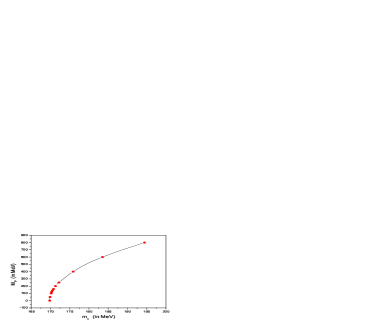
Figure 1: Evolution of the pseudoscalar meson mass with quark mass $m_{u}$.

Below we consider $\ell=0$, the pseudoscalar ($J^{PC}=0^{-+}$) and vector ($1^{--}$) mesons, the most established sectors of hadron spectroscopy.

For the ground state mass $M=M_{0}$ we obtain:

$$1 = {\alpha_{s}\Lambda^{4}\over 48\pi m_{1}^{2}m_{2}^{2}}~{}\exp\left\{{M^{2}(\mu_{1}^{2}+\mu_{2}^{2})-m_{1}^{2}-m_{2}^{2}\over 2\Lambda^{2}}\right\}\max\limits_{1/3<b<1}\left\{\left[{(5\,b-1)(1-b)\over b}\right]^{2}\right.$$ (11)

$$\!\!\!\!\!\cdot\exp\left[-{b\,M^{2}(\mu_{1}-\mu_{2})^{2}\over 4\Lambda^{2}}\right]\left[2\,b\,\rho_{J}+{M^{2}\over\Lambda^{2}}\left(\mu_{1}\,\mu_{2}+b\,(2-b\,\rho_{j}){(\mu_{1}-\mu_{2})^{2}\over 4}\right)\right.$$

$$\!\!\!\!\!\left.\left.+{m_{1}m_{2}\over\Lambda^{2}}\left(1+\chi_{J}~{}\omega\left({m_{1}\over\Lambda}\right)\omega\left({m_{2}\over\Lambda}\right)\right)\right]\right\}\,,$$

where $\omega(z)=1/(1+z^{2}/4)$ and

$$\rho_{J}=\left\{1,1/2\right\}\,,~{}~{}~{}\chi_{J}=\left\{+1,-1\right\}~{}~{}~{}\mbox{\rm for}~{}~{}~{}J=\{P,V\}\,.$$

Equation (11) is nontrivial, the behaviour of the quark propagator $\tilde{S}\sim 1/m^{2}$ imposes a restriction on the value of the quark mass from below. Particularly, the evolution of the pseudoscalar meson mass $M_{P}(m_{u},m_{u})$ with ”constituent-quark” mass $m_{u}$ at fixed values of $\{\alpha_{s},\Lambda\}$ is depicted in Fig.1. The optimal value of $m_{u}$ is fixed from the relation $M_{P}(m_{u},m_{u})=M_{\pi}=138$ MeV.

By comparing our estimates with the observed meson masses [8] we have found the following optimal values of free parameters [7]:

$$\alpha_{s}=0.186\,,\qquad\Lambda=730{\mbox{\rm~{}MeV}}\,,\qquad m_{ud}=170{\mbox{\rm~{}MeV}}\,,$$

$$m_{s}=188{\mbox{\rm~{}MeV}}\,,\qquad m_{c}=646{\mbox{\rm~{}MeV}}\,,\qquad m_{b}=4221{\mbox{\rm~{}MeV}}\,.$$ (12)

$J^{PC}=0^{-+}$	$M_{P}$	$J^{PC}=0^{-+}$	$M_{P}$	$J^{PC}=1^{--}$	$M_{V}$	$J^{PC}=1^{--}$	$M_{V}$
$\pi(138)$	138	$D(1870)$	1928	$\rho(770)$	813	$K^{*}(892)$	927
$\eta(547)$	508	$D_{s}(1970)$	2009	$\omega(782)$	826	$D^{*}(2010)$	2028
$\eta_{c}(2979)$	3018	$B(5279)$	5359	$\Phi(1019)$	1041	$D^{*}_{s}(2112)$	2106
$\eta_{b}(9300)$	9458	$B_{s}(5370)$	5397	$J/\Psi(3097)$	3097	$B^{*}(5325)$	5361
$K(495)$	495	$B_{c}(6286)$	6074	$\Upsilon(9460)$	9460

Table 1: Estimated ground-state masses $M_{P}$ and $M_{V}$ (in MeV).

Our estimates for the pseudoscalar and vector meson masses in the ground state (Tab.1 and Fig.2) compared with experimental data show that the relative error is small ($\sim 1\div 5$ per cent) in a wide range of mass $\sim 140\div 9500{\mbox{\rm~{}MeV}}$.

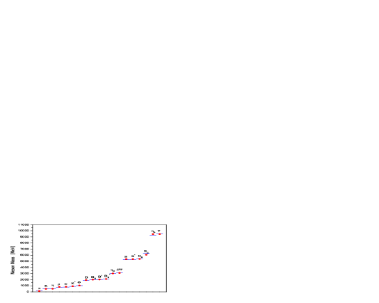
Figure 2: The estimated meson masses (dots) and the experimental data (dashes).

We note:

1. The set of optimal parameters (12) is not unique, another set also gives a reasonable ground-state spectra for $P$ and $V$ mesons. But we choose these values by taking into account other important hadron data such as the orbital and radial excitations of mesons as well as the lowest-state glueball mass.

2. The obtained value $\alpha_{s}=0.186$ is in agreement with the latest experimental data for the QCD coupling value $\alpha_{s}^{QCD}\approx 0.10\div 0.35$ on the hadron distance [8] and with the prediction of the quenched theory $\alpha_{s}^{quench}\approx 0.195$ [10]. Moreover, this relatively weak coupling value justifies the use of the one-gluon exchange mode in our consideration. A possible use of a ”sliding” interaction strength $\alpha_{s}(M)$ depending on the mass scale (see, e.g., [11, 12, 10]) will be discussed later.

3. The obtained quark masses fit an hierarchy: $m_{u,d}<m_{s}<m_{c}<m_{b}$.

4. Our model provides the $SU(3)$-symmetry breaking: $M_{\pi}\not=M_{K}$.

5. The $\omega$ and $\Phi$ mesons considered as mixed states of $u\bar{u}+d\bar{d}$ and $s\bar{s}$ pairs with a priori unknown mixing angle $\theta_{V}$. The optimal value is found: $\theta_{V}=9^{\circ}$.

6. The $U(1)$-splitting is explained, i.e., we obtain a large mass difference $M_{\pi}/M_{\eta}\approx 0.25$ between pseudoscalar isovector and isoscalar mesons, while $M_{\rho}/M_{\omega}\approx 1$ for the vector isovector and isoscalar.

7. The dependence of the meson masses $M(m_{1}+m_{2})$ on the sum of two ”constituent” quark masses (Fig.3) is nontrivial.

8. A rough estimate of the hadronization region

   $$r_{hadr}^{2}\sim{\int d^{4}x~{}x^{2}~{}D(x)\over\int d^{4}x~{}x~{}D(x)}={8\over\Lambda^{2}}\sim\left({1\over 250\mbox{\rm MeV}}\right)^{2}$$

   shows that the confinement scale $r_{conf}\simeq 1/\Lambda$ is comparable with $r_{hadr}$.

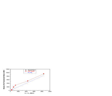
Figure 3: The estimated masses for the $P$ and $V$ mesons versa the sum of quark masses. The dashed straight lines depict the plain sum $m_{1}+m_{2}$.

Below, we extend our consideration to the orbital ($\ell>0$) and radial ($n_{r}>0$) excitations of mesons.

4 Meson Regge Trajectories with $n_{r}=0$

The orbital excitations take place in larger distances and should be less sensitive to the short-range details of the propagators. Therefore, correct description of the meson Regge trajectories can serve as an additional test ground for our model.

Below we concentrate mostly on the orbital excitations with zero radial number $n_{r}=0$ for which experimental data exist for all states with $\ell\leq 5$.

Particularly, by substituting (9) into (7) we obtain the mass equation:

$$1\!\!\! = \!\!\!{\alpha_{s}\Lambda^{4}\over 48\pi m_{1}^{2}m_{2}^{2}}{1\over 4^{\ell}({\ell}+1)!}~{}\exp\left\{{(m_{1}^{2}+m_{2}^{2})\over 2\Lambda^{2}}\left[{M_{\ell}^{2}\over(m_{1}+m_{2})^{2}}-1\right]\right\}$$ (13)

$$\!\!\!\!\!\cdot\max\limits_{1/3<c<1}\left\{\left[{(5\,c-1)(1-c)\over c^{2}}\right]^{2}~{}\left(c^{2}{d\over dc}\right)^{\ell}\left\{c^{2}\exp\left[-{c\,M_{\ell}^{2}(m_{1}-m_{2})^{2}\over 4\Lambda^{2}(m_{1}+m_{2})^{2}}\right]\right.\right.$$

$$\!\!\!\!\!\cdot\left[2\,c\,\rho_{J}+{M_{\ell}^{2}\over\Lambda^{2}(m_{1}+m_{2})^{2}}\left(m_{1}\,m_{2}+{c\,(2-c\,\rho_{j})\over 4}~{}(m_{1}-m_{2})^{2}\right)\right.$$

$$\!\!\!\!\!\left.\left.\left.+{m_{1}\,m_{2}\over\Lambda^{2}}\left(1+\chi_{J}~{}\omega\left({m_{1}\over\Lambda}\right)\omega\left({m_{2}\over\Lambda}\right)\right)\right]\right\}\right\}\,,$$

where $\omega(z)=1/(1+z^{2}/4)$ and $\rho_{J}=\left\{1,1/2\right\}\,,~{}~{}\chi_{J}=\left\{+1,-1\right\}~{}~{}\mbox{\rm for}~{}~{}J=\{P,V\}\,$.

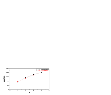
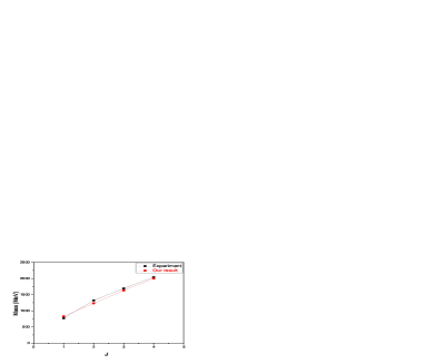
Figure 4: The estimated mass $M_{J}$ (dots) for the $\rho$- and $K^{*}$-meson excitations.

Substituting the optimal parameters (12) into (13) we have estimated the masses of excitations for the $\rho$-meson and $K$-meson families. Our estimates (dots) plotted versa the quantum number $J=\ell+s$  ($s=\{0,1\}$ - the spin of the $(q\bar{q^{\prime}})$ pair) is given in Fig.4 in comparison with the experimental data (boxes) [8].

As is expected, our model describes acceptably the $J$-trajectories of the $\rho$-meson and $K$-meson excitations.

For large $\ell\gg 1$ the asymptotical behaviour of $M_{\ell}^{2}$ reads

$$M_{\ell}^{2}\simeq 4(m_{1}+m_{2})^{2}+4\Lambda^{2}(\ell+2)\ln\left({2\over 3-\sqrt{5}}\right)=M_{0}^{2}+\ell\cdot\Omega_{\ell}\,.$$ (14)

We note that for large $J\gg 1$:

i) The Regge trajectories of $K^{*}$ and $\rho$ mesons are linear and similar.

ii) The intercept $M_{0}^{2}$ is positive and depends on quark masses and $\Lambda$.

ii) The slope $\Omega_{\ell}$ sensitively depends only on $\Lambda$.

5 Meson Radial Excitations $n_{r}>0$

A nice example of the meson radial excitations is the ”charmonium” sector. Experimentally well established is the $J/\Psi$-family $(c\bar{c})$ with $J^{PC}=1^{--}$.

We expand the radial part of the normalized trial function as follows:

$$U_{n}(x)\sim L_{n}^{(1/2)}(2b\vec{x}^{2})\exp\left\{-\Lambda^{2}(b\vec{x}^{2}+cx_{0}^{2})\right\}\,,\qquad\int\!dx\left|U_{n}(x)\right|^{2}=1\,,\qquad x=\{x_{0},\vec{x}\}\,,$$

where $\{b,c\}$ – dimensionless positive parameters, $n$ – the radial quantum number and $L_{n}^{(1/2)}(z)$ is the generalized Laguerre polynomial.

Taking into account the orthogonality of $L_{n}^{(1/2)}(z)$ on the interval $(0,\infty)$ with respect to the weight function $w(z)=z^{1/2}~{}e^{-z}$ we arrive in the equation for the radial-excitation spectrum:

$$1\!\!\! = \!\!\!{\alpha_{s}\over 48\sqrt{\pi}}\left({\Lambda\over m}\right)^{4}\exp\left\{{M_{n}^{2}\over 4\Lambda^{2}}-{m^{2}\over\Lambda^{2}}\right\}~{}{1\over n!(n+1)!}~{}\max\limits_{A,B}\left\{\left[{{(5A-1)(1-A)\over A}}\right]^{1/2}\right.$$ (15)

$$\!\!\!\!\!\left.\cdot~{}(2B-1)^{3/2}{d^{2n}\over dt^{n}ds^{n}}\left[{A+{3\,u\,v\over u\,v+u+v}+{M_{n}^{2}\over\Lambda^{2}}+{4\,m^{2}\over\Lambda^{2}}(1-\omega^{2}({m/\Lambda}))\over[(1-t)(1-s)(u\,v+u+v)]^{3/2}}\right]\right\}_{t=0,~{}s=0}\,,$$

where

$$u=B+{(2B-1)\,s\over(1-s)}\,,~{}~{}~{}~{}v=B+{(2B-1)\,t\over(1-t)}\,,~{}~{}~{}~{}~{}~{}{1\over 3}<A<1<B<\infty\,.$$

The numerical solutions of Eq.(15) for $M_{n}(c\bar{c})$ are plotted in Fig.5. We see that there exists an expressed convexity for $n<3$ and for higher mass members the $n$-trajectory is approximately linear. By analysing (15) for large $n$ we obtain the solution:

$$M_{n}^{2}(m,\Lambda)=M_{0}^{2}(m,\Lambda)+n\cdot\Omega_{n}(\Lambda)\,.$$ (16)

For $n\gg 1$:

i) The radial Regge trajectories are linear.

ii) The intercept $M_{0}^{2}$ depends on both $m$ and $\Lambda$.

ii) The slope $\Omega_{n}$ depends only on $\Lambda$.

Figure 5: The spectrum of the $J/\Psi$-family radial excitations for $\Lambda=730~{}{\mbox{\rm MeV}}$.

Note, for the $1^{--}$ radial excitations of charmonium, we obtain a correct (convex, asymptotically linear) behaviour, but underestimate the experimental data. For larger $\Lambda\sim 800\div 850~{}{\mbox{\rm MeV}}$ our estimate approaches the results in [8].

6 Glueball Lowest State

In contrast to the meson sector, the experimental status of the glueball is not clear. The signatures naively expected for glueballs in the experiment are: the absence in any ($q\bar{q}$) nonets, an enhanced production in gluon-rich channels of central productions and radiative decays, a decay branching fraction incompatible with two-quark states and the reduced couplings.

There are predictions expecting non-$q\bar{q}$ scalar objects, like glueballs and multiquark states in the mass range $\sim 1600\div 1800{\mbox{\rm~{}MeV}}$ [13, 14]. Recent lattice calculations, QCD sum rules, ”tube” and constituent glue models agree that the lightest glueballs have quantum numbers $J^{PC}=0^{++}$ and $2^{++}$.

A QCD sum rule [15] and the K-matrix analysis [16] predict the scalar glueball mass $M_{G}=1.25\pm 0.2{\mbox{\rm~{}GeV}}$ reducing down the quantized knot soliton model result [17] and the earlier quenched lattice estimates $M_{G}\simeq 1550{\mbox{\rm~{}MeV}}$ [18, 19, 20]. However, most recent quenched lattice estimate with improved action favors a larger mass close to $M_{G}=1710\pm 50\pm 58{\mbox{\rm~{}MeV}}$ [21].

It is evident that the structure of QCD vacuum plays the main role in the formation of glueballs. We suppose that the lowest state of the glueball may be reasonably described by the ”gluon-gluon” bound state $J^{PC}=0^{++}$ in our model.

The Gaussian character of the gluon propagator (2) allows us explicitly solve the equation for the glueball mass and the result reads:

$$M_{G}^{2}=2\Lambda^{2}\ln\left({\alpha_{upp}\over\alpha_{s}}\right)\,,\qquad\alpha_{upp}={2\pi(2+\sqrt{3})^{2}\over 27}\,.$$ (17)

Note, the glueball mass (17) depends on $\alpha_{s}$ in a nonperturbative way and the physical restriction $M_{G}^{2}\geq 0$ leads to an upper bound: $\alpha_{s}<\alpha_{upp}\approx 3.24124$.

Substituting the optimal parameters ($\alpha_{s}=0.186,~{}\Lambda=730{\mbox{\rm~{}MeV}}$) obtained for the meson sector into (17) we estimate the lowest-state scalar glueball mass

$$M_{G}=1745{\mbox{\rm~{}MeV}}\,.$$ (18)

Our estimate (18) does not contradict the latest predictions expecting glueballs in the mass range $\sim 1600\div 1800{\mbox{\rm~{}MeV}}$ [13, 14].

In conclusion, we have considered a relativistic quantum field model of interacting quarks and gluons under the analytic confinement. We have used only physical parameters (the quark masses, the coupling constant and the confinement scale) for the model and solved the Bethe-Salpeter equation in the ladder approximation for the hadron bound states. The use of one-gluon exchange mode is justified by the estimated small value $\alpha_{s}=0.186$ of the coupling constant that is also in agreement with both the prediction of the quenched theory $\alpha_{quenched}\approx 0.195$ [10] and the latest experimental data for the QCD running coupling $\alpha_{s}\approx 0.10\div 0.35$.

Our approach does not require the ”flux tube”-type confinement for the light and heavy mesons.

Within a simple relativistic model with reasonable forms of the quark and gluon propagators we describe correctly:

- the pseudoscalar and vector meson masses in the ground state and orbital excitations. The relative error is small in a wide range of mass $140{\mbox{\rm~{}MeV}}\div 9.46{\mbox{\rm~{}GeV}}$,

- the quark mass hierarchy: $m_{u,d}<m_{s}<m_{c}<m_{b}$,

- the SU(3)-symmetry breaking: $M_{K}\not=M_{\pi}$,

- the so-called ”$U(1)$-splitting”: $M_{\pi}\ll M_{\eta}$ while $M_{\rho}\approx M_{\omega}$,

- the approximately linear radial and orbital Regge trajectories for the pseudoscalar and vector mesons,

- the lowest state glueball mass close to $\sim 1750{\mbox{\rm~{}MeV}}$.

The author thanks V.V.Burov, G.V.Efimov, S.B.Gerasimov, E.Klempt and W.Oelert for useful discussions and comments.

References

- [1] M. Baldicchi and G.M. Prospri, arXiv:hep-ph/0310213 (2003).
- [2] P. Maris and C.D. Roberts, Int. J. Mod. Phys., E12 (2003) 297.
- [3] H. Leutwyler, Phys. Lett., 96B (1980) 154; Nucl. Phys., B179 (1981) 129.
-
[4]
G.V. Efimov and S.N. Nedelko, Phys. Rev., D51 (1995) 174;
Ja.V. Burdanov et al., Phys. Rev., D54 (1996) 4483. - [5] G.V. Efimov and G. Ganbold, Phys. Rev., D65 (2002) 054012.
- [6] G. Ganbold, AIP Conf. Proc., 717 (2004) 285.
- [7] G. Ganbold, AIP Conf. Proc., 796 (2005) 127; arXiv:hep-ph/0512287 (2005).
- [8] Particle Data Group, W.M- Yao et al., J. Phys., G33 (2006) 1.
- [9] T. Feldman, Int. J. Mod. Phys., A15 (2000) 159.
- [10] O. Kaszmarek and F. Zantow, Phys. Rev., D71 (2005) 114510.
- [11] D.V. Shirkov, Theor. Math. Phys., 132 (2002) 484.
- [12] A.V. Nesterenko, Int. J. M. Phys., A18 (2003) 5475.
- [13] C. Amsler, N.A. Tornqvist, Phys. Rep., 389 (2004) 61.
- [14] D.V. Bugg, Phys. Lett., C397 (2004) 257.
- [15] H. Forkel, Phys. Rev., D71 (2005) 054008.
- [16] V.V. Anisovich, AIP Conf. Proc., 717 (2004) 441; arXiv:hep-ph/0310165 (2004).
- [17] K.-I. Kondo et al., arXiv:hep-th/0604006 (2006).
- [18] G. Bali et. al., Phys. Lett., B309 (1993) 378;
- [19] C. Morningstar and M. Peardon, Phys. Rev., D60 (1999) 034509.
- [20] W. Lee and D. Weingarten, Phys. Rev., D61 (2000) 014015.
- [21] Y. Chen et. al., Phys. Rev., D73 (2006) 014516.