Nature of the $f_{0}(600)$ from its $N_{c}$ dependence at two loops in unitarized Chiral Perturbation Theory

Abstract

By using unitarized two-loop Chiral Perturbation Theory partial waves to describe pion-pion scattering we find that the dominant component of the lightest scalar meson does not follow the $\bar{q}q$ dependence on the number of colors that, in contrast, is obeyed by the lightest vectors. The method suggests that a subdominant $\bar{q}q$ component of the $f_{0}(600)$ possibly originates around 1 GeV.

The lightest scalar mesons are a subject of a longstanding controversy that is recently receiving relevant contributions that could help settling the questions about their existence and nature. Experimentally, several analyses Aitala:2000xu , find poles for the $f_{0}(600)$ and $\kappa$, the lightest scalars with isospin 0 and 1/2, respectively. The former is of interest for spectroscopy but also for understanding spontaneous chiral symmetry breaking, since it has precisely the vacuum quantum numbers. On the theoretical side, the QCD chiral symmetry breaking pattern has been shown to lead to $f_{0}(600)$ and $\kappa$ poles in $\pi\pi$ and $\pi K$ scattering newsigma ; VanBeveren:1986ea ; Dobado:1996ps ; Oller:1997ti ; Oller:1997ng . Concerning the spectroscopic classification, the caveat for most hadronic models is the difficulty to extract the quark and gluon composition without assumptions hard to justify within QCD. In contrast, when using fundamental degrees of freedom, i.e., in lattice or with QCD inspired potentials, other complications arise, related to chiral symmetry breaking, the use of actual quark masses or the physical pion or kaon masses and decay constants. All approaches are also complicated by the possible mixing of different states in the physical one. Most of these caveats are overcome in a recent approach Pelaez:2003dy (Pelaez:2004xp for a review) based on the pole dependence on the number of colors, $N_{c}$, of meson-meson scattering within unitarized Chiral Perturbation Theory.

The relevance of the large $N_{c}$ expansion 'tHooft:1973jz is that it provides an analytic approximation to QCD in the whole energy region and a clear identification of $\bar{q}q$ states, that become bound states as $N_{c}\rightarrow\infty$, and whose masses scale as $O(1)$ and their widths as $O(1/N_{c})$. Other kind of hadronic states may show different behaviors Jaffe .

In order to avoid any spurious $N_{c}$ dependence in the hadronic description, we use Chiral Perturbation Theory (ChPT), which is the QCD low energy Effective Theory, and where the large $N_{c}$ behavior is implemented systematically. It is built as the most general derivative expansion of a Lagrangian chpt1 , in terms of $\pi,K$ and $\eta$ mesons compatible with the QCD symmetries, These particles are the Goldstone bosons associated to the spontaneous chiral symmetry breaking of massless QCD and are therefore the lightest degrees of freedom. Actually, the $u$, $d$ and $s$ quark masses are non-vanishing but small enough to be treated as perturbations that give rise to $\pi,K$ and $\eta$ masses. Thus, ChPT is an expansion in powers of momenta and masses and, generically, its applicability is limited to a few hundred MeV above threshold. Each order is made of all possible terms multiplied by a “chiral” parameter. These Low Energy Constants (LECS) are renormalized to absorb loop divergences order by order, and once determined from experiment they can be used in any other pseudo-Goldstone boson amplitude.

For our purposes, we are interested in meson-meson scattering amplitudes, since by unitarization they generate dynamically resonances not initially present in ChPT Truong:1988zp ; Dobado:1996ps ; Oller:1997ng ; Guerrero:1998ei ; GomezNicola:2001as ; Oller:1997ti . Indeed GomezNicola:2001as ; Pelaez:2004xp , with the coupled channel Inverse Amplitude Method (IAM), the one loop ChPT meson-meson amplitudes describe data up to roughly $\sqrt{s}\simeq 1.2\,$GeV and generate the $\rho$ and $K^{*}$ vectors, as well as the $f_{0}(600)$, $\kappa$, $a_{0}(980)$ and $f_{0}(980)$ scalars, and, most importantly, using LECS compatible with standard ChPT and therefore without any further assumption or source of spurious $N_{c}$ dependence.

By scaling the one-loop ChPT parameters with their $N_{c}$ behavior, it was recently shown that the generated $\rho$ and $K^{*}$ show the typical $N_{c}$ behavior of $\bar{q}q$ states, whereas the scalars are at odds with a dominant $\bar{q}q$ component. These results, confirmed by other methods Uehara:2003ax , implied some cancellation between tree level diagrams proportional to LECS, and that loop diagrams with two intermediate mesons are very relevant in the generation of light scalars. But such loop diagrams are subdominant in the large $N_{c}$ counting and one could wonder about the stability under small changes in the LECS and about higher order ChPT corrections that could become larger than loop terms at sufficiently large $N_{c}$, and reveal the existence of subdominant $\bar{q}q$ components.

Here we present a method to quantify the above statements, and generalize the approach of Pelaez:2003dy to two-loop ChPT and in particular to $\pi\pi$ scattering Bijnens:1997vq . Despite the many second order parameters and their large uncertainties, the data can be well described and we find once more that the $\rho(770)$ behaves as $\bar{q}q$ with $N_{c}$, whereas the $f_{0}(600)$ main component does not behave as such. Furthermore, with the second order calculation a dominant $\bar{q}q$ behavior cannot be imposed on the $f_{0}(600)$ and the $\rho$ simultaneously, but a subdominant $\bar{q}q$ $f_{0}(600)$ component seems to arise at larger $N_{c}$ around $1$ GeV.

Thus, at leading order, the only parameter is the pion decay constant in the chiral limit, $f_{0}=O(\sqrt{N_{c}})$, fixed by the spontaneous symmetry breaking scale $4\pi f_{0}\simeq 1\,$GeV. Indeed, ChPT $\pi\pi$ scattering amplitudes are expanded as $t\simeq t_{2}+t_{4}+t_{6}+\,\ldots$ with $t_{k}=O((p/4\pi f_{0})^{k})$ and are, generically, $O(1/N_{c})$. In particular, the LECS appearing in $\pi\pi$ scattering at $O(p^{4})$ chpt1 , all scale as $O(N_{c})$. For simplicity we use the $SU(2)$ notation, $l_{i}^{r}$, since we are only dealing with $\pi\pi$ scattering (see the last reference in chpt1 for a translation to $SU(3)$). In Table I we give a sample of $l_{i}^{r}$ sets given in the literature, whose differences we take as systematic uncertainties for the set we use in our fits below. In Table II we also list the six $O(p^{6})$ constants that appear in $\pi\pi$ scattering, denoted $r_{i}$. They all count as $O(N_{c}^{2})$. Those values are just estimates assuming they are saturated by the multiplets of the lightest (predominantly vector) resonances. This hypothesis works well at $O(p^{4})$ Ecker:1988te , but for $O(p^{6})$ is probably just correct within an order of magnitude Bijnens:1997vq and we conservatively assign a 100% uncertainty.

	$O(p^{4})$ LECS				$O(p^{6})$ LECS
Refs.	chpt1	BijnensGasser	Pelaez:2004xp	we use	Amoros:1999qq	Bijnens:1997vq	Girlanda:1997ed	we use
$10^{3}l_{1}^{r}$	-6.0	-5.4	-3.5	3.5$\pm$2.2	-3.3	-5.2	-4.6	-3.3$\pm$2.2
$10^{3}l_{2}^{r}$	5.5	5.7	4.7	4.7$\pm$1.0	2.9	2.3	2.0	2.9$\pm$1.0
$10^{3}l_{3}^{r}$	0.82	0.82	-2.6	0.82$\pm$3.8	1.2	0.82	0.82	0.82$\pm$3.8
$10^{3}l_{4}^{r}$	5.6	5.6	8.6	6.2$\pm$2.0	2.4	5.6	6.2	6.2$\pm$2.0

Table 1: Sample of LECS central values. The fifth and ninth columns, whose uncertainties roughly represent the previous sample, are used in our fits in the text to calculate $\chi^{2}_{LECS}$.

The large $N_{c}$ counting does not specify at what renormalization scale $\mu$ it applies, thus becoming an uncertainty studied in Pelaez:2003dy for the one-loop LECS. For the $r_{i}$, the scale dependence is much more cumbersome and has not been written explicitly. Nevertheless, in both cases it is subleading in $1/N_{c}$, and given the fact that we have a 100% error on the $r_{i}$ should be well within errors for our fits. Hence, we do not perform such analysis here, simply setting $\mu=770\,$MeV, as usual.

Next, resonances can be found as poles in partial wave amplitudes $t_{IJ}$ of isospin $I$ and angular momentum $J$ that, in the elastic regime satisfy the unitarity condition:

$${\mbox{Im}\,}t=\sigma|t|^{2}\Rightarrow{\mbox{Im}\,}\frac{1}{t}=-\sigma\Rightarrow t=\frac{1}{{\mbox{Re}\,}t^{-1}-i\sigma},$$ (1)

where $\sigma$ is the known two-meson phase space and we have omitted the $IJ$ indices for brevity. Note that ChPT expansions violate exact unitarity, since in the first Eq.(1), the highest power of momenta on the right hand is twice that on the left. Unitarity is only satisfied perturbatively

$${\mbox{Im}\,}t_{2}=0,\quad{\mbox{Im}\,}t_{4}=\sigma t_{2}^{2},\quad{\mbox{Im}\,}t_{6}=\sigma 2t_{2}{\mbox{Re}\,}t_{4},\;\ldots$$ (2)

If we replace in Eq.(1) ${\mbox{Re}\,}t^{-1}$ by its ChPT approximation we get the Inverse Amplitude Method (IAM), that satisfies elastic unitarity exactly. At $O(p^{4})$ it reads,

$$t\simeq t_{2}^{2}/(t_{2}-t_{4}),$$ (3)

and its fit to “data only” is listed in Table II, in the SU(2) notation. The fit quality is remarkable, given the huge systematic uncertainties, (conservatively $\pm 5^{0}$ and 5% error for the $f_{0}(600)$ channel) and we refer to GomezNicola:2001as ; Pelaez:2004xp for details and figures with a comparison with data. Using Eqs.(1) and (2), the $O(p^{6})$ IAM Dobado:1996ps ; Nieves:2001de reads

$$t\simeq t_{2}^{2}/(t_{2}-t_{4}+t_{4}^{2}/t_{2}-t_{6}),$$ (4)

that recovers the $O(p^{6})$ ChPT expansion at low energies and describes well elastic $\pi\pi$ scattering data Nieves:2001de . In addition, the IAM has a right cut that defines two Riemann sheets. In the second sheet we find poles associated to resonances; in particular, for the $\rho(770)$ in the $(I,J)=(1,1)$ channel and for the $f_{0}(600)$ in the $(0,0)$ one. For narrow resonances, $\Gamma<<M$, the pole position is related to its mass and width as $\sqrt{s_{\rm pole}}\simeq M-i\Gamma/2$, and we keep this as a definition for the wide $f_{0}(600)$, whose $M\sim 400-500\,$MeV and $\Gamma\sim 400-600\,$MeV.

By scaling the previous parameters with their dominant $N_{c}$ behavior, namely, $f_{N_{c}}\rightarrow f\sqrt{N_{c}/3}$, $l^{r}_{i,\,N_{c}}\rightarrow l_{i}^{r}N_{c}/3$ and $r_{i,\,N_{c}}\rightarrow r_{i}(N_{c}/3)^{2}$, we obtain the large $N_{c}$ dependence of $M_{N_{c}}$ and $\Gamma_{N_{c}}$ of the $\rho$ and $f_{0}(600)$ poles generated by the IAM. If a resonance is predominantly a $\bar{q}q$, $M_{N}\sim O(1)$ and $\Gamma_{N}\sim O(1/N_{c})$, and so it was shown Pelaez:2003dy that the $O(p^{4})$ IAM reproduced remarkably well that behavior for the $\rho(770)$ and $K^{*}(892)$, two well established $\bar{q}q$ mesons. This is the expected behavior if in Eq.(3) one neglects the two-meson loop terms, which are subleading at large $N_{c}$ with respect to $O(p^{4})$ LECS contributions.

In contrast, the lightest scalars follow a qualitatively different behavior. Loop diagrams, instead of the $O(p^{4})$ LECS terms, play a relevant role in determining the scalar pole position. This is nothing but the well known fact that light scalars are dynamically generated by the resummation in Eq.(3) of two-meson loop diagrams Dobado:1996ps ; Guerrero:1998ei ; GomezNicola:2001as ; Oller:1997ti ; Oller:1997ng . However, although relevant at $N_{c}=3$, loop diagrams are suppressed by $1/N_{c}$ compared to tree level terms with LECS, and the $O(p^{6})$ terms could become bigger at some larger $N_{c}$, where the $O(p^{4})$ $N_{c}$ results should no longer be trusted. For that reason it is important to check the $O(p^{6})$ IAM: it should give small corrections to the $O(p^{4})$ close to $N_{c}=3$, but it may deviate at larger $N_{c}$ and even unveil some subdominant $\bar{q}q$ component.

Still, before scaling the $O(p^{6})$ IAM, let us first note that $M_{N_{c}}=O(1)$ and $\Gamma_{N_{c}}=O(1/N_{c})$ is only the leading $\bar{q}q$ scaling. Taking into account subleading uncertainties, to consider a resonance a $\bar{q}q$ state, it is enough that

$$M_{N_{c}}^{\bar{q}q}=\widetilde{M}\left(1+\frac{\epsilon_{M}}{N_{c}}\right),\;\Gamma_{N_{c}}^{\bar{q}q}=\frac{\widetilde{\Gamma}}{N_{c}}\left(1+\frac{\epsilon_{\Gamma}}{N_{c}}\right),$$ (5)

were $\widetilde{M}$ and $\widetilde{\Gamma}$ are unknown but $N_{c}$ independent and the subleading terms have been gathered in $\epsilon_{M},\epsilon_{\Gamma}$, which are $O(1)$. Thus, for a $\bar{q}q$ state, the expected $M_{N_{c}}$ and $\Gamma_{N_{c}}$ can be obtained from those at $N_{c}-1$ generated by the IAM,

$$M_{N_{c}}^{\bar{q}q} \simeq M_{N_{c}-1}\left[1+\epsilon_{M}\left(\frac{1}{N_{c}}-\frac{1}{N_{c}-1}\right)\right]$$

$$\equiv M_{N_{c}-1}+\Delta M^{\bar{q}q}_{N_{c}},$$

$$\Gamma_{N_{c}}^{\bar{q}q} \simeq \frac{\Gamma_{N_{c}-1}\,(N_{c}-1)}{N_{c}}\left[1+\epsilon_{\Gamma}\left(\frac{1}{N_{c}}-\frac{1}{N_{c}-1}\right)\right]$$

$$\equiv \frac{\Gamma_{N_{c}-1}\,(N_{c}-1)}{N_{c}}+\Delta\Gamma_{N_{c}}^{\bar{q}q}.$$

Note the $\bar{q}q$ index for all quantities obtained assuming a $\bar{q}q$ behavior. We refer the values at $N_{c}$ to those at $N_{c}-1$ because then we will be able to calculate from what $N_{c}$ value a resonance starts behaving as a $\bar{q}q$, which is of interest in order to look for subdominant $\bar{q}q$ components. Thus, we can now define an averaged $\bar{\chi}_{\bar{q}q}^{2}$to measure how close a resonance is to a $\bar{q}q$ behavior, using as uncertainty the $\Delta M^{\bar{q}q}_{N_{c}}$ and $\Delta\Gamma_{N_{c}}^{\bar{q}q}$.

$$\bar{\chi}_{\bar{q}q}^{2}\!=\!\frac{1}{2n}\sum_{N_{c}=4}^{n}\!\left[\left(\frac{M_{N_{c}}^{\bar{q}q}-M_{N_{c}}}{\Delta M_{N_{c}}^{\bar{q}q}}\right)^{\!\!2}\!\!+\left(\frac{\Gamma_{N_{c}}^{\bar{q}q}-\Gamma_{N_{c}}}{\Delta\Gamma_{N_{c}}^{\bar{q}q}}\right)^{\!\!2}\right]$$ (8)

Since at $N_{c}=3$ we expect generically 30% uncertainties we take $\epsilon_{M}=\epsilon_{\Gamma}=1$. Let us note that $\Delta M$, and even faster $\Delta\Gamma$, tend to zero for large $N_{c}$ and eventually become smaller than our precision determining the pole position, 1 MeV, which we add as a systematic error. When a state is predominantly $\bar{q}q$, it should follow Eq.(5) and $\bar{\chi}_{\bar{q}q}^{2}\mathrel{\lower 2.5pt\vbox{\hbox{$<$}\hbox{$\sim$}}}1$. Otherwise $\bar{\chi}_{\bar{q}q}^{2}\gg 1$. Note that $n$ should not be too far from 3, since we are looking for the $N_{c}$ behavior of the physical state. If we took $n$ too large, we could be changing radically the original mixture of the observed state and for sufficiently large $N_{c}$ even the tiniest $\bar{q}q$ component could become dominant over the rest Sun:2005uk . Therefore, our method first determines the behavior of the resonance dominant component, but also, when $\bar{q}q$ is not dominant, the $N_{c}$ at which it becomes so.

Furthermore, by minimizing its $\bar{\chi}_{\bar{q}q}^{2}$ we can constrain a state to follow the $\bar{q}q$ behavior. Thus, we will minimize $\chi^{2}_{data}+\chi^{2}_{LECS}$ plus the $\bar{\chi}_{\bar{q}q}^{2}$ of either of the $\rho$, or the $f_{0}(600)$, or both. The averaged $\chi^{2}_{LECS}$ measures how far the fitted LECS are from their typical values in the tables and stabilizes them. Note that $\pi\pi$ scattering data are poor, with large systematic uncertainties and not very sensitive to some of the individual parameters but to their combinations, thus producing large correlations, driving the LECS away from the typical values for tiny improvements in the $\chi^{2}$, particularly at $O(p^{6})$. We will provide the $\chi^{2}_{data}$, $\chi^{2}_{LECS}$, and $\bar{\chi}_{\bar{q}q}^{2}$, divided by the number of data points, the number of LECS and $2n$, respectively.

Thus, in Table II we show three $O(p^{4})$ fits: to data only, constrained to a $\rho$ $\bar{q}q$ hypothesis, or constraining the $f_{0}(600)$ to be a $\bar{q}q$. We list for each fit the different $\chi^{2}$ described above and we see that our approach clearly identifies the $\rho$ as a $\bar{q}q$, since $\bar{\chi}_{\rho,\bar{q}q}^{2}\simeq 0.25$. In contrast, $\bar{\chi}_{\bar{q}q}^{2}\geq 125$ for the $f_{0}(600)$, even if we constrain the fit to minimize also $\bar{\chi}_{\bar{q}q}^{2}$ for the $f_{0}(600)$ (at the price of a higher $\chi^{2}_{LECS}=5.6$). This is the quantitative statement of the $O(p^{4})$ results in Pelaez:2003dy ; Pelaez:2004xp where it was concluded that the main component of the $f_{0}(600)$ was not $\bar{q}q$.

Unfortunately, the $O(p^{6})$ analysis has a large freedom and thus $\chi^{2}_{LECS}$ plays a relevant role to stabilize the fit, but keeping in mind that the $r_{i}$ uncertainties were arbitrarily chosen to be 100%. In Table II and Fig. 1 we show three $O(p^{6})$ fits: constraining the $\rho$ as a $\bar{q}q$ (Fig. 1. Top), or the $f_{0}(600)$ (Fig. 1. Center) or both (Fig. 1, Bottom). As expected, the $O(p^{6})$ results are consistent with those at $O(p^{4})$ not far from $N_{c}=3$ Pelaez:2003dy ; Pelaez:2004xp but for the scalar channel they deviate around $N_{c}\sim 8$.

In particular, in the “$\rho$ as $\bar{q}q$” fit a $\bar{q}q$ dominant nature comes out neatly for the $\rho$, whose $\bar{\chi}_{\bar{q}q}^{2}\sim 0.9$, but is discarded for the $f_{0}(600)$, since its $\bar{\chi}_{\bar{q}q}^{2}\simeq 15$ and Fig.1 shows that its mass and width both rise when $N_{c}$ increases not too far from real life, $N_{c}=3$. However, for $N_{c}>8$ the mass tends to a constant around 1 GeV and the width decreases, but not with a $1/N_{c}$ scaling. This suggests a mixing with a $\bar{q}q$ subdominant component, arising as loop-diagrams become more suppressed at large $N_{c}$.

	fits $O(p^{4})$			fits $O(p^{6})$
Fit	Only	$\rho$ as	$f_{0}(600)$	$\rho$ as	$f_{0}(600)$	$\rho,f_{0}(600)$
	data	$\bar{q}q$	as $\bar{q}q$	$\bar{q}q$	as $\bar{q}q$	as $\bar{q}q$
$10^{3}l_{1}$	-3.8	-3.8	-3.9	-5.4	-5.7	-5.7
$10^{3}l_{2}$	4.9	5.0	4.6	1.8	2.6	2.5
$10^{3}l_{3}$	0.43	0.42	2.6	1.5	-1.7	0.39
$10^{3}l_{4}$	7.2	6.4	15	9.0	1.7	3.5
$\chi^{2}_{data}$	1.1	1.2	1.4	1.1	1.4	1.5
$\chi^{2}_{LECS}$	0.08	0.03	5.6	1.9	2.1	1.4
$\chi^{2}_{\rho,\bar{q}q}$	0.26	0.22	0.32	0.93	2.0	1.3
$\chi^{2}_{f_{0}(600),\bar{q}q}$	140	143	125	15	3.5	4.0
$10^{4}r_{1}$		-0.6		-0.60	-0.60	-0.58
$10^{4}r_{2}$		1.3	Our	1.5	1.3	1.5
$10^{4}r_{3}$	Ref.	-1.7	$O(p^{6})$	-1.4	-4.4	-3.2
$10^{4}r_{4}$	Bijnens:1997vq	-1.0	fits	1.4	-0.03	-0.49
$10^{4}r_{5}$		1.1		2.4	2.7	2.7
$10^{4}r_{6}$		0.3		-0.60	-0.70	-0.62

Table 2: IAM fits to data or constrained to a $\bar{q}q$ $N_{c}$ behavior for the $\rho$ and $f_{0}(600)$. In boldface the $\chi^{2}$ minimized on each fit. For the $O(p^{6})$ fits we also provide the $r_{i}$ estimates Bijnens:1997vq

One might wonder if the $f_{0}(600)$ could also be forced to behave predominantly as a $\bar{q}q$. Thus we made a “$f_{0}(600)$ as a $\bar{q}q$” constrained fit (Fig. 1, Center). The price to pay is a deterioration of the $\chi^{2}_{data}$ and an unacceptable $\rho$ $\bar{q}q$ behavior, since its $\bar{\chi}_{\bar{q}q}^{2}\sim 2$. Still, the $f_{0}(600)$ $\bar{\chi}_{\bar{q}q}^{2}$ decreases only to $3.5$ (for 34 $N_{c}$ points). This extreme case allows us to conclude that the $O(p^{6})$ calculation cannot accommodate a $\bar{q}q$ dominant component for the $f_{0}(600)$.

Finally, we have studied how much of a subdominant $\bar{q}q$ behavior the $f_{0}(600)$ can accommodate without spoiling that of the $\rho$. Hence, we have also minimized in the fit the $\bar{\chi}_{\bar{q}q}^{2}$ both for the $\rho$ and $f_{0}(600)$ (Fig. 1, Bottom). The $f_{0}(600)$ still does not behave predominantly as a $\bar{q}q$, since its $\bar{\chi}_{\bar{q}q}^{2}\simeq 4$. However, it starts behaving as a $\bar{q}q$, i.e., $\bar{\chi}_{\bar{q}q}^{2}\simeq 1$, for $N_{c}\geq 6$. The $\bar{q}q$ behavior of the $\rho$ only deteriorates a little, $\bar{\chi}_{\bar{q}q}^{2}\simeq 1.3$, and should not be pushed much further. This result suggests that the subdominant mixing with a $\bar{q}q$ state around 1 GeV seen in the first fit, would become dominant around $N_{c}>6$, at best .

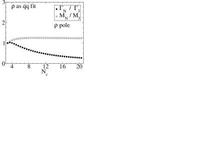
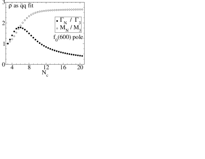
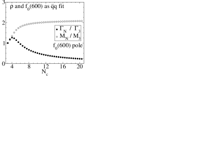
Figure 1: Mass and width $N_{c}$ behavior of the $\rho$ and $f_{0}(600)$ from an $O(p^{6})$ IAM data fit minimizing also the $\bar{\chi}_{\bar{q}q}^{2}$: of the $\rho$ (Top). of the $f_{0}(600)$ instead of the $\rho$ (Center) of both the $f_{0}(600)$ and $\rho$ (Bottom).

In summary, we have presented a method to determine quantitatively how close the $N_{c}$ dependence of a resonance pole is to a $\bar{q}q$ behavior. We have applied this measure to the poles generated in $\pi\pi$ scattering by unitarized Chiral Perturbation Theory, which is the effective low energy theory of QCD and reproduces systematically its large $N_{c}$ expansion. The method is able to confirm the $O(p^{4})$ qualitative results Pelaez:2003dy ; Pelaez:2004xp , identifying the $\rho$ as a $\bar{q}q$ state and showing that the $f_{0}(600)$ is at odds with a dominant $\bar{q}q$ component. We have extended the method to $O(p^{6})$ confirming the stability of our $O(p^{4})$ conclusions, but also showing that a possible subdominant $\bar{q}q$ may originate around 1 GeV. This provides further support, based on the QCD $N_{c}$ dependence, to some models that generate the $f_{0}(600)$ from final state meson interactions, and locate a “preexisting” $\bar{q}q$ scalar nonet VanBeveren:1986ea ; Oller:1997ti around 1 GeV. The methods presented here should be easily generalized to investigate the nature of other dynamically generated mesons Dobado:2001rv and baryons GomezNicola:2000wk .

References

- (1) E. M. Aitala et al. [E791 Collaboration], Phys. Rev. Lett. 86, 770 (2001) Phys. Rev. Lett. 89, 121801 (2002) I. Bediaga and J. M. de Miranda, Phys. Lett. B 633, 167 (2006) M. Ablikim et al. [BES Collaboration], Phys. Lett. B 598, 149 (2004) D. V. Bugg, Phys. Lett. B 572, 1 (2003) [Erratum-ibid. B 595, 556 (2004)], Phys. Rept. 397, 257 (2004).
- (2) R.L. Jaffe, Phys. Rev. D15 267 (1977); Phys. Rev. D15, 281 (1977). R. Kaminski, L. Lesniak and J. P. Maillet, Phys. Rev. D 50 (1994) 3145. M. Harada, F. Sannino and J. Schechter, Phys. Rev. D 54 (1996) 1991 R. Delbourgo and M. D. Scadron, Mod. Phys. Lett. A 10 (1995) 251. S. Ishida et al., Prog. Theor. Phys. 95 (1996) 745; Prog. Theor. Phys. 98,621 (1997). N. A. Tornqvist and M. Roos, Phys. Rev. Lett. 76 (1996) 1575. D. Black et al.,. Phys. Rev. D58:054012,1998. G. Colangelo, J. Gasser and H. Leutwyler, Nucl. Phys. B 603, 125 (2001)
- (3) E. Van Beveren, et al. Z. Phys. C 30, 615 (1986) and hep-ph/0606022. E. van Beveren and G. Rupp, Eur. Phys. J. C 22 (2001) 493, hep-ph/0201006.
- (4) A. Dobado and J. R. Pelaez, Phys. Rev. D 47 (1993) 4883. Phys. Rev. D 56 (1997) 3057.
- (5) J. A. Oller and E. Oset, Nucl. Phys. A 620 (1997) 438; [Erratum-ibid. A 652 (1999) 407] Phys. Rev. D 60 (1999) 074023.
- (6) J. A. Oller, E. Oset and J. R. Pelaez, Phys. Rev. Lett. 80 (1998) 3452; Phys. Rev. D 59 (1999) 074001 [Erratum-ibid. D 60 (1999) 09990], and Phys. Rev. D 62 (2000) 114017. M. Uehara, hep-ph/0204020.
- (7) J. R. Pelaez, Phys. Rev. Lett. 92, 102001 (2004)
- (8) J. R. Pelaez, Mod. Phys. Lett. A 19, 2879 (2004)
- (9) G. ’t Hooft, Nucl. Phys. B 72 (1974) 461. E. Witten, Annals Phys. 128 (1980) 363.
- (10) R. L. Jaffe, Proceedings of the Intl. Symposium on Lepton and Photon Interactions at High Energies. Physikalisches Institut, University of Bonn (1981) . ISBN: 3-9800625-0-3
- (11) S. Weinberg, Physica A96 (1979) 327. J. Gasser and H. Leutwyler, Annals Phys. 158 (1984) 142; Nucl. Phys. B 250 (1985) 465.
- (12) T. N. Truong, Phys. Rev. Lett. 61 (1988) 2526. Phys. Rev. Lett. 67, (1991) 2260; A. Dobado, M.J.Herrero and T.N. Truong, Phys. Lett. B235 (1990) 134.
- (13) F. Guerrero and J. A. Oller, Nucl. Phys. B 537 (1999) 459 [Erratum-ibid. B 602 (2001) 641].
- (14) A. Gómez Nicola and J. R. Peláez, Phys. Rev. D 65 (2002) 054009 and AIP Conf. Proc. 660 (2003) 102 [hep-ph/0301049].
- (15) M. Uehara, hep-ph/0308241, hep-ph/0401037, hep-ph/0404221.
- (16) J. Bijnens et al.,Nucl. Phys. B 508, 263 (1997)
- (17) G. Amoros, J. Bijnens and P. Talavera, Phys. Lett. B 480, 71 (2000)
- (18) J. Bijnens, G. Colangelo and J. Gasser, Nucl. Phys. B427 (1994) 427.
- (19) L. Girlanda, M. Knecht, B. Moussallam and J. Stern, Phys. Lett. B 409, 461 (1997) J. Nieves and E. Ruiz Arriola, Eur. Phys. J. A 8, 377 (2000)
- (20) G. Ecker, J. Gasser, A. Pich and E. de Rafael, Nucl. Phys. B 321, 311 (1989). J. F. Donoghue, C. Ramirez and G. Valencia, Phys. Rev. D 39, 1947 (1989).
- (21) J. Nieves, M. Pavon Valderrama and E. Ruiz Arriola, Phys. Rev. D 65, 036002 (2002)
- (22) Z. X. Sun, et al. hep-ph/0503195. J. R. Pelaez, hep-ph/0509284.
- (23) A. Dobado and J. R. Pelaez, Phys. Rev. D 65, 077502 (2002) L. Roca, E. Oset and J. Singh, Phys. Rev. D 72, 014002 (2005)
- (24) A. Gomez Nicola, J. Nieves, J. R. Pelaez and E. Ruiz Arriola, Phys. Lett. B 486, 77 (2000)