Evolution of Critical Correlations at the QCD Phase Transition

Abstract

We investigate the evolution of the density-density correlations in the isoscalar critical condensate formed at the QCD critical point. The initial equilibrium state of the system is characterized by a fractal measure determining the distribution of isoscalar particles (sigmas) in configuration space. Non-equilibrium dynamics is induced through a sudden symmetry breaking leading gradually to the deformation of the initial fractal geometry. After constructing an ensemble of configurations describing the initial state of the isoscalar field we solve the equations of motion and show that remnants of the critical state and the associated fractal geometry survive for time scales larger than the time needed for the mass of the isoscalar particles to reach the two-pion threshold. This result is more transparent in an event-by-event analysis of the phenomenon. Thus, we conclude that the initial fractal properties can eventually be transferred to the observable pion-sector through the decay of the sigmas even in the case of a quench.

I Introduction

Experiments of a new generation, with relativistic nuclei, at RHIC and SPS are currently under consideration with the aim to intensify the search for the existence and location of the QCD critical point in the phase diagram of strongly interacting matter RIKEN ; Antoncern . Important developments in lattice QCD karsch and studies of hadronic matter at high temperatures Antoniou2003 suggest that the QCD critical endpoint is likely to be located within reach at SPS energies. It is therefore desirable to explore the range of baryon number chemical potential $\mu_{B}=$100-500 MeV by studying collisions at relatively low energies, $\sqrt{s}\simeq\,$5-20 GeV per nucleon pair. A decisive observation, in these experiments, associated with the development of a second-order phase transition at the critical endpoint of QCD matter is the establishment of power laws in momentum space (self similarity) in close analogy to the phenomenon of critical opalescence in QED matter lesne . These power laws reflect the fractal geometry of real space, and a characteristic index of the critical behavior is the fractal mass dimension $D_{f}$ which measures the strength of the order-parameter fluctuations within the universality class of critical QCD Antoniou2001 .

The physics underlying the endpoint singularity in the QCD phase diagram is associated with the phenomenon of chiral phase transition, a fundamental property of strong interactions in the limit of zero quark masses. In this case and for a given chemical potential $\mu_{B}$ there exists a critical temperature $T_{cr}$ above which chiral symmetry is restored and as temperature decreases below $T_{cr}$, the system enters into the chirally broken phase of observable hadrons. It is believed that, for two flavors and zero quark masses, there is a first-order phase transition line on the $(T,\mu_{B})$ surface at large $\mu_{B}$ RW1 . This line ends at a tricritical point beyond which the phase transitions become of second order. In the case of real QCD with non-zero quark masses, chiral symmetry is broken explicitly and the first-order line ends at a critical point beyond which the second-order transitions are replaced by analytical crossovers bergraja99 .

The order parameter of the chiral phase transition is the chiral field $\Phi=(\sigma,\vec{\pi})$ formed by the scalar, isoscalar field $\sigma$ together with the pseudoscalar, isovector field $\vec{\pi}=(\pi^{+},\pi^{0},\pi^{-})$. Both fields are massless at the tricritical point and when the symmetry is restored at high temperatures, their expectation value vanishes, $\langle\vec{\pi}\rangle=\langle\sigma\rangle=0$. However, in the presence of an explicit symmetry breaking mechanism (non-zero quark masses) the pion and sigma fields are disentangled at the level of the order parameter of the QCD critical point, which is now formed by the sigma field alone. The expectation value of the $\sigma$-field remains small but not zero near the critical point so that the chiral symmetry is never completely restored. The valuable observables in this case are associated with the fluctuations of the $\sigma$-field, $(\delta\sigma)^{2}\simeq\langle\sigma^{2}\rangle$, and they incorporate, in principle, the singular behavior of baryon-number susceptibility and in particular the power-law behavior of the $\sigma$-field correlator hatta03 .

The aim of this work is to study the evolution of critical correlations during the development of the collision, in the neighborhood of the QCD critical point. In the initial state we assume that the system has reached the critical point in thermal equilibrium so the $\sigma$-field fluctuations are described by the $3-D$ Ising critical exponent $\delta$ and in particular by the fractal dimension $D_{f}=\frac{3\delta}{\delta+1}$ ($\delta\simeq 5$). The crucial question from the observational point of view is whether in the freeze-out regime, which follows the equilibration stage, the relaxation time-scale $\tau_{rel}$ of these fluctuations is long enough compared to the time-scale $\tau_{th}$ associated with the development of a massive $\sigma$-field beyond the two-pion threshold ($m_{\sigma}\geq 2m_{\pi}$). Both time-scales ($\tau_{rel},\tau_{th}$) are characteristic parameters of the out-of-equilibrium phenomena ($\sigma$ rescattering) which take place during the evolution of the system (towards freeze-out) and the requirement $\tau_{rel}\gg\tau_{th}$ guarantees that critical fluctuations may become observable in the $\sigma$-mode ($\sigma\rightarrow\pi^{+}\pi^{-}$ Antoniou2001 ; Fuj ).

In order to quantify these effects, we adopt in this work the picture of a rapid expansion (quench) which is a realistic possibility in the framework of heavy-ion collisions. We study the out-of-equilibrium evolution of the initial fractal characteristics of the $\sigma$-field and we search for time scales $\tau_{rel},\tau_{th}$ satisfying the above constraint in a particular class of events (event-by-event search). The dynamics of the system is fixed by a two-field Lagrangian, $\mathcal{L}(\sigma,\vec{\pi})$, together with appropriate initial conditions. The out-of-equilibrium phenomena are generated by the exchange of energy between the $\sigma$-field and the environment which consists of massive pions initially in thermal equilibrium.

In section II the formulation of the problem and in particular the equations of motion, the initial conditions and the generation of thermal $\pi$-configurations are presented. In section III numerical solutions of the evolution of critical fluctuations are given and discussed whereas in section IV our final results and conclusions are summarized.

II Formulation of $\sigma$ field dynamics

In our approach we assume an initial critical state of the system in thermal equilibrium, disturbed by a two-field potential $V(\sigma,\vec{\pi})$, in an effective description inspired by the chiral theory of strong interactions GL ; RW . The 3-dimensional Lagrangian density is

$$\mathcal{L}=\frac{1}{2}(\partial_{\mu}\sigma\partial^{\mu}\sigma+\partial_{\mu}\vec{\pi}\partial^{\mu}\vec{\pi})-V(\sigma,\vec{\pi})$$ (1)

with the potential

$$V(\sigma,\vec{\pi})=\frac{\lambda^{2}}{4}(\sigma^{2}+\vec{\pi}^{2}-v_{0}^{2})^{2}+\frac{m_{\pi}^{2}}{2}\left(\vec{\pi}^{2}-2v_{0}\sigma+2v_{0}^{2}\right),$$ (2)

where $\sigma=\sigma(\vec{x},t)$ and $\vec{\pi}=\vec{\pi}(\vec{x},t)$. The potential has the usual $\sigma$-model form plus a term which breaks the symmetry along the $\sigma$-direction. With the addition of the mass term for the pion field, we ensure that it has a constant mass equal to $m_{\pi}$. Finally, the constant terms in (2) shift to zero the value of the potential at the minimum. We fix the parameters of the Lagrangian using the phenomenological values $m_{\pi}$$\approx 139\,$ MeV and $v_{0}\approx 87.4\,$ MeV, whereas the known uncertainty in the phenomenological value of zero temperature $\sigma$-mass, given by $m_{\sigma}=\sqrt{2\lambda^{2}v_{0}^{2}}$, yields $10\lesssim\lambda^{2}\lesssim 20$ for $400\lesssim m_{\sigma}\lesssim 600\,$ MeV.

The equations of motion resulting from (1) are:

$$\ddot{\sigma}-\nabla^{2}\sigma+\lambda^{2}(\sigma^{2}+\vec{\pi}^{2}-v_{0}^{2})\sigma=v_{0}m_{\pi}^{2}$$

$$\ddot{\vec{\pi}}-\nabla^{2}\vec{\pi}+\lambda^{2}(\sigma^{2}+\vec{\pi}^{2}-v_{0}^{2})\vec{\pi}+m_{\pi}^{2}\vec{\pi}=0,$$ (3)

where $\vec{\pi}^{2}=(\pi^{+})^{2}+(\pi^{0})^{2}+(\pi^{-})^{2}$.

Using a constant value $v_{0}$ in eq. 2 implies a non-vanishing mass (finite correlation length) for the $\sigma$-field, $m_{\sigma}=\sqrt{2\lambda^{2}v_{0}^{2}}$, in contradiction with its critical profile. This inconsistency is restored if we assume a finite-time mechanism instead of the instant quench i.e the instantaneous formation of the potential (2) at $t=0$. The simplest model which leaves the equations of motion unaffected, used also in cosmological phase transitions Rivers , is the so-called linear quench SRS2 . It assumes that the minimum $v$ of the potential increases linearly with time, starting from zero and ending at the zero temperature value $v_{0}\approx 87.4\,$ MeV after a time interval $\tau$ which is the quench duration:

$$v(t)=v_{0}t/\tau\text{\ \ \ \ \ \ \ \ \ \ for \ \ \ \ \ $t\leq\tau$}$$

$$v(t)=v_{0}\text{\ \ \ \ \ \ \ \ \ \ \ \ \ \ for \ \ \ \ \ $t>\tau$}.$$ (4)

In this way we acquire $m_{\sigma}=0$ at $t=0$, as expected for the critical $\sigma$-field and, with increasing time, $m_{\sigma}$ approaches its zero temperature value.

To proceed numerically we have to discretize eqs. (3) on a lattice. We use the following leap-frog discretization scheme:

$$\sigma^{n+2}_{i,j,k}=2\sigma^{n+1}_{i,j,k}-\sigma^{n}_{i,j,k}+\frac{dt^{2}}{\alpha^{2}}\left\{\left[\sigma^{n+1}_{i+1,j,k}+\sigma^{n+1}_{i-1,j,k}-2\sigma^{n+1}_{i,j,k}\right]+\left[\sigma^{n+1}_{i,j+1,k}+\sigma^{n+1}_{i,j-1,k}-2\sigma^{n+1}_{i,j,k}\right]+\ \ \ \ \ \ \ \ \right.$$

$$\left.\ \ \ \ \ \ \ \ \ \ \ \ \ \ \ \ \ \ \ \ \ \ \ \ \ \left[\sigma^{n+1}_{i,j,k+1}+\sigma^{n+1}_{i,j,k-1}-2\sigma^{n+1}_{i,j,k}\right]\right\}-dt^{2}\left\{\lambda^{2}\left[\left(\sigma^{n+1}_{i,j,k}\right)^{2}+\left(\vec{\pi}^{n+1}_{i,j,k}\right)^{2}-v^{2}\right]\sigma^{n+1}_{i,j,k}-vm_{\pi}^{2}\right\},$$ (5)

and similarly for the other three equations considering the $\pi$-field. In eq. (5) $\alpha$ is the lattice spacing while $dt$ is the time step. The upper indices indicate the time instants and the lower indices the lattice sites. As usual we perform an initial fourth order Runge-Kutta step to make our algorithm self-starting, and we impose periodic boundary conditions.

We are interested in studying the evolution of the above system using initial field configurations dictated by the onset of the critical behavior. In this case we expect that the $\sigma$-field, being the order parameter, will possess critical fluctuations, and the $\pi$-fields to be thermal, while the entire system will be in thermodynamical and chemical equilibrium. Obviously, the subsequent evolution, determined by eqs. (3), will generate strong deviations from equilibrium. Before going on with the detailed study of the dynamics, we first describe in the following subsections the generation of an ensemble of field configurations on a 3-D lattice possessing the characteristics of the critical system. This ensemble enters in the subsequent analysis as the initial condition.

II.1 Generation of initial ensemble of critical $\sigma$-configurations

The absolute value of the $\sigma$-field introduced in the previous subsection is interpreted as local density, and the corresponding critical behavior is described by a fractal measure demonstrated in the dependence of the mean ”mass” $M(\vec{x}_{0},R)$ on the distance $R$ around a point $\vec{x}_{0}$ defined by:

$$M(\vec{x}_{0},R)=\langle\int_{R}|\sigma(\vec{x})\sigma(\vec{x}_{0})|\,d^{D}x\rangle,$$ (6)

obeying the power law

$$M(\vec{x}_{0},R)\sim R^{D_{f}}$$ (7)

for every $\vec{x}_{0}$. $D_{f}$ is the fractal mass dimension of the system Mandel83 ; Vicsek ; Falconer and the mean value is taken with respect to the ensemble of the initial $\sigma$-configurations. The production of the $\sigma$ configurations building up the critical ensemble, characterized by the fractal measure given in eqs. (6,7), has been accomplished in Antoniou98 . In fact the fractal properties of the critical system can be produced as an ensemble average, through the partition function:

$$Z=\int{\cal{\delta}}[\sigma]e^{-\Gamma[\sigma]},$$ (8)

with $\Gamma[\sigma]$ the scale invariant effective action at $T=T_{cr}$, $\mu=\mu_{cr}$:

$$\Gamma[\sigma]=\int_{R}d^{D}x\{\frac{1}{2}(\nabla\sigma)^{2}+g\sigma^{\delta+1}\}.$$ (9)

The sum over field configurations in (8) can be saturated through saddle point solutions of $\Gamma[\sigma]$, which consist approximately of piecewise constant configurations extended over domains of variable size. A detailed description of the corresponding simulation algorithm is given in manoscomput . Using this algorithm, after averaging, the mean ”mass” in the ensemble satisfies eq. (7) with a fractal mass dimension

$$D_{f}=\frac{D\delta}{\delta+1}.$$ (10)

For the 3-D Ising universality class, $D=3$, the isothermal critical exponent is $\delta\approx 5$, and the coupling $g\approx 2$ Tsypin , therefore $D_{f}\approx 5/2$.

The power-law behavior of $M(\vec{x}_{0},R)=\langle\int_{R}|\sigma(\vec{x})\sigma(\vec{x}_{0})|\,d^{3}x\rangle$ around a random $x_{0}$, averaged inside clusters of volume $V$, is illustrated in fig. 1.

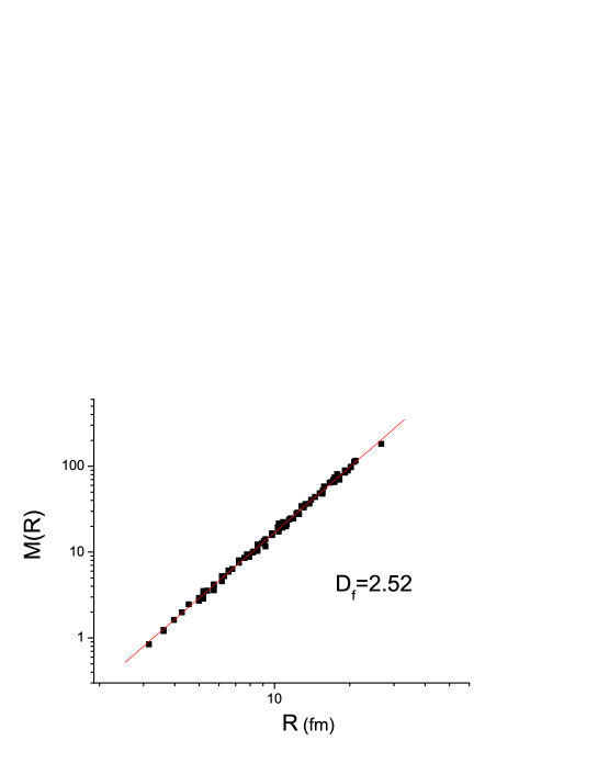
Figure 1: $M(R)=\langle\int_{R}|\sigma(\vec{x})\sigma(\vec{x}_{0})|\,d^{3}x\rangle$ versus $R$ for the ensemble of $\sigma$-field configurations. The slope $\Psi$, i.e the fractal mass dimension $D_{f}$ is equal to $5/2$ within an error of less than 1%.

The $M(\vec{x}_{0},R)$ versus $R$ figure is drawn as follows: For a given $\vec{x}_{0}$ of a specific configuration we find $R$ of the cluster in which it belongs, taken $\simeq\sqrt[3]{V}$, and we calculate the integral $\int|\sigma(\vec{x})\sigma(\vec{x}_{0})|\,d^{3}x$, thus acquiring one point in the $M(\vec{x}_{0},R)$ vs $R$ figure. For the same $\vec{x}_{0}$ we repeat this procedure until we cover the whole ensemble, and the aforementioned figure is formed. Averaging in $\vec{x}_{0}$ leads only to a slight modification of the result, since $M(\vec{x}_{0},R)\approx M(\vec{x}_{0}+\vec{l},R)$, with $\vec{l}$ spanning the entire lattice, therefore in the following we replace $M(\vec{x}_{0},R)$ by $M(R)$. We observe that in the log-log plot of $M(R)$ vs $R$, the slope $\Psi$, i.e the fractal mass dimension $D_{f}$ according to (7), deviates from the theoretically expected value of $5/2$ by less than 1%. Furthermore, the mean value of the $\sigma$-field (spatial average) is almost zero as expected to happen near the critical point.

With this procedure we acquire an ensemble of field configurations and the expected power law arises as a statistical property after ensemble averaging manoscomput . Alternatively, one could extend the notion of the fractal dimension using individual configurations, where the quantity of interest is the exponent $d_{f}$ of the power law of the integral

$$m(R)=\int_{R}|\sigma(\vec{x})\sigma(\vec{x}_{0})|\,d^{3}x\,d^{3}x_{0}\sim R^{d_{f}}.$$ (11)

Calculating $d_{f}$ for each configuration we obtain a distribution around $5/2$ with standard deviation $\approx 0.05$. As expected the ensemble average of $d_{f}$ is $\langle d_{f}\rangle=D_{f}$, within an error of less than 0.5%.

II.2 Generation of initial thermal $\pi$-configurations

We generalize the method of Cooper in order to produce an ensemble of 3-D $\pi$-configurations in real space, corresponding to an ideal gas at temperature $T_{0}$. The unperturbed Hamiltonian for the classical scalar field theory in three dimensions is

$$H=\frac{1}{2}\int d^{3}x[(\partial_{t}\pi(\vec{x},t))^{2}+(\nabla\pi(\vec{x},t))^{2}+m_{\pi}^{2}\pi(\vec{x},t)^{2}].$$ (12)

The free particle solutions for $t=0$ are

$$\pi(\vec{x},0)=\int^{+\infty}_{-\infty}\frac{d^{3}k}{(2\pi)^{3}}\pi_{k0}\,e^{i\vec{k}\vec{x}}=\int^{+\infty}_{-\infty}\frac{d^{3}k}{(2\pi)^{3}}\frac{(a_{k}+a_{-k}^{\ast})}{\sqrt{2\omega_{k}}}e^{i\vec{k}\vec{x}}$$

$$\dot{\pi}(\vec{x},0)=\int^{+\infty}_{-\infty}\frac{d^{3}k}{(2\pi)^{3}}\xi_{k0}\,e^{i\vec{k}\vec{x}}=\int^{+\infty}_{-\infty}\frac{d^{3}k}{(2\pi)^{3}}\sqrt{\frac{\omega_{k}}{2}}i(a_{-k}^{\ast}-a_{k})e^{i\vec{k}\vec{x}}.$$ (13)

where $\omega_{k}=\sqrt{k^{2}+m_{\pi}^{2}}$.

Now, choosing an initial classical density distribution Cooper

$$\rho[\pi,\dot{\pi}]=Z^{-1}(\beta_{0})\,\exp{\left\{-\beta_{0}\,H[\pi,\dot{\pi}]\right\}},$$

and substituting the Hamiltonian (12) with the free particle solutions (13), we finally get

$$\rho[x_{k},y_{k}]=Z^{-1}(\beta_{0})\,\exp{\left\{-\beta_{0}\,\int^{+\infty}_{-\infty}\frac{d^{3}k}{(2\pi)^{3}}\omega_{k}(x_{k}^{2}+y_{k}^{2})\right\}},$$ (14)

with $\beta_{0}=1/T_{0}$, and where: $a_{k}=x_{k}+iy_{k}$ with $x_{k},y_{k}$ real. In order to produce a thermal ensemble (at temperature $T_{0}$) of configurations for $\pi(\vec{x},0)$ and $\dot{\pi}(\vec{x},0)$, we select $x_{k}$ and $y_{k}$ from the gaussian distribution (14), assemble $a_{k}$ and then substitute in (13). Lastly, since we have three components of the pion pseudoscalar field, we independently repeat this procedure accordingly. All the characteristics of the $\pi$-ensemble such as the correlation function $\langle\pi(\vec{x})\pi(\vec{x}+\delta\vec{x})\rangle-\langle\pi(\vec{x})\rangle\langle\pi(\vec{x}+\delta\vec{x})\rangle$, which turns out to be a $\delta$-function, are consistent with the assumption of an ideal thermal gas.

III Numerical Solutions

We study the evolution of the system determined by equations (3) which we solve in 3-D $25\times 25\times 25$ lattice, using as initial conditions an ensemble of $10^{4}$ independent $\sigma$-configurations on the lattice generated as described above, i.e possessing fractal characteristics, and $10^{4}$ configurations for each $\pi$ component corresponding to an ideal gas at temperature $T_{0}\approx 140$ MeV. The initial time derivatives of the $\sigma$-field, forming the kinetic energy, are assumed to be zero, since this is a strong requirement of the initial equilibrium. The used population is by far satisfactory since the results converge for ensembles with more than $7\times 10^{3}$ configurations (numerically tested) for the considered lattices (sizes from $15\times 15\times 15$ to $25\times 25\times 25$ sites). In addition, we find that the obtained results are independent of the lattice spacing $\alpha$ despite the discontinuities in the derivatives of the piecewise constant configurations, as the corresponding variation $\delta\sigma$ goes to zero fast enough so that the limit $\lim_{\alpha\rightarrow 0}\frac{\delta\sigma}{\alpha}$ exists manoscomput . Lastly, varying the value of $T_{0}$ between 100 MeV and 180 MeV it has a negligible effect on the results. We investigate the evolution of $M(R)$ of the whole ensemble which initially follows a power law $\sim R^{\Psi(0)}$ with $\Psi(0)\equiv D_{f}=5/2$. We also study the evolution of $m(R)$ for each configuration. At $t=0$ $m(R)$ possess a power-law behavior of the form $\sim R^{\psi(0)}$, with the exponent $\psi(0)\equiv d_{f}$ normally distributed around $5/2$ (with standard deviation $\approx 0.05$).

We evolve the system for various $\lambda^{2}$, corresponding to different $m_{\sigma}$ values at $T=0$, and for various quench times $\tau$. In figs. 2 and 3 we demonstrate the evolution of the mean field values $\langle\sigma\rangle$ and $\langle\pi^{+}\rangle$ (the other components are similar), where the averages are taken over all statistically independent configurations.

Figure 2: Time evolution of the mean field value $\langle\sigma\rangle$ for various $\lambda^{2}$ and $\tau$ cases.

Figure 3: Time evolution of the mean field value $\langle\pi\rangle$ for various $\lambda^{2}$ and $\tau$ cases.

As expected $\langle\sigma\rangle$ oscillates around the potential minimum which relaxes after $\tau$, while $\langle\pi^{+}\rangle$ stays around zero due to the absence of a linear in $\vec{\pi}$ term in the potential (2).

In fig. 4 we present $M(R)$ vs $R$ for three successive times and we observe that the slope $\Psi(t)$ fluctuates, leading to a distortion of the initial fractal geometry.

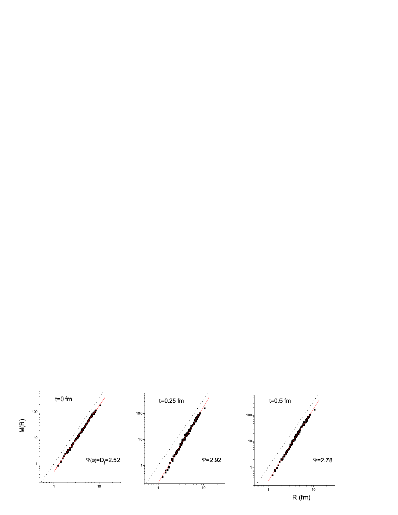
Figure 4: $M(R)$ vs $R$ for three successive times, $t=0$ fm, $t=0.25$ fm and $t=0.5$ fm, for typical $\lambda^{2}$ and $\tau$ values. The solid lines mark the power-law fit, and the dotted line has slope $2.5$ and is used as a reference.

In fig. 5 we depict the evolution of the slope $\Psi(t)$ of $M(R)$ versus $R$ (each $\Psi(t)$ value obtained trough a linear fit), for the same $\lambda^{2}$ and $\tau$ values as before.

Figure 5: Time evolution of $\Psi(t)$ (solid line) and $\langle\Psi\rangle_{t}$ (dashed line) for the whole ensemble, for the same $\lambda^{2}$ and $\tau$ cases as before. The vertical line marks the time $t=\tau_{th}$ where $m_{\sigma}$ reaches the threshold $2m_{\pi}$.

With the dashed line we plot the time average of $\Psi(t)$ defined by $\langle\Psi\rangle_{t}=\frac{1}{t}\int_{0}^{t}\Psi(t^{\prime})dt^{\prime}$. We observe the remarkable phenomenon that the characteristic exponent $\Psi(t)$ after reaching the value of the embedding dimension 3, it fluctuates and for particular times it becomes almost equal to $\Psi(0)=5/2$. Thus, after the first deformation, the initial critical behavior of the whole ensemble is partially restored and deformed repeatedly. A detailed explanation of this revival is given in deterministic . The key point is that the partial restoration takes place when $\langle\sigma(t)\rangle$ passes through its lower turning point, where the $\sigma$-field (seen as a system of coupled oscillators) reaches a state similar to the initial one. This phenomenon weakens gradually, and finally the dynamics dilutes completely the initial critical behavior.

This phenomenon is also visible in the evolution of the slope $\psi(t)$ of $m(R)$ versus $R$, for each configuration. Indeed, in fig. 6 we demonstrate the evolution of the mean field value as well as of $\psi$ and of its time average, for $\lambda^{2}=20$ and $\tau=1$ fm, for three independent configurations of the ensemble, corresponding to initial value $\psi(0)=d_{f}$ equal to 2.51, 2.50 and 2.53 respectively.

Figure 6: $\langle\sigma\rangle$, $\psi(t)$ (solid line) and $\langle\psi\rangle_{t}$ (dashed line) for three independent configurations, for $\lambda^{2}=20$ and $\tau=1$ fm. The vertical line marks the time $t=\tau_{th}$ where $m_{\sigma}$ reaches the threshold $2m_{\pi}$.

We observe an oscillatory behavior of $\psi(t)$ similar to that of $\Psi(t)$ of the whole ensemble presented in fig. 5.

In a heavy ion collision, if the fireball passes near the critical point we expect $\sigma$ to have almost zero mass. As the system expands, its temperature decreases, $v$ increases towards its zero temperature value $v_{0}$ and $m_{\sigma}=\sqrt{2\lambda^{2}v(t)^{2}}$ tends to its freeze out value. However, when it reaches the threshold $m_{\sigma}=2m_{\pi}$, at time $t=\tau_{th}$, it starts decaying into pions, and the decay rate of $\sigma\rightarrow\pi^{+}\pi^{-}$, being proportional to the available phase space parameter $\sqrt{1-\frac{4m_{\pi}^{2}}{m_{\sigma}^{2}}}$, becomes larger as $m_{\sigma}$ increases. So if the critical characteristics of $\sigma$ have survived at that threshold, they can be transferred to the produced pions, leaving signatures of the critical point at the detectors. Note here that these pions are not affected by the thermal ones which constitute the environment. In figs. 5 and 6 the vertical line depicts the threshold time $t=\tau_{th}$. We are interested in investigating the time averaged measures after this threshold since these quantities are observable.

The first measure one has to look at is the evolution of $\Psi(t)$ and $\langle\Psi\rangle_{t}$ for the whole ensemble, after $t=\tau_{th}$, as it is shown in fig. 5. As we observe these vary between 2.6 and 2.9, for the various $\lambda^{2}$ and $\tau$ values, offering weak traces of the initial power law of 5/2. This cogitation is amplified by the fact that if we evolve our system with conventional initial conditions ($D_{f}\approx 3$), then $\Psi(t)$ and $\langle\Psi\rangle_{t}$ remain always $\approx 3$, as we have tested, supporting the assumptions that slopes $<2.9$ indicate initial critical behavior. However, slopes close to 3 could originate from conventional strong processes leading to power-law correlations with very small intermittency exponents Bialas86 . Therefore we have to refer to more sophisticated measures in order to acquire a direct observation of the QCD isothermal critical exponent $\delta$, independently of the specific model. One way to achieve this is to perform event-by-event analysis of our results.

As we have mentioned, we use an ensemble of $\sigma$-field configurations, each one possessing its own $d_{f}$ which can vary, leading to a distribution with mean value $\approx 5/2$ and standard deviation $\approx 0.05$. An event-by-event analysis of the system evolution consists in calculating the percentage $P$ of the initial configurations (all of which have $\psi(0)=d_{f}\approx 5/2$) that possess again this value at time $t$ (actually we count those with $2.4<\psi(t)<2.6$). Obviously, $P(t)$ leads to experimentally accessible effects after $t=\tau_{th}$. In fig. 7 we depict the evolution of $P(t)$, and its time average $\langle P\rangle_{t}$ for $t>\tau_{th}$ (the vertical line marks $t=\tau_{th}$), for the same $\lambda^{2}$ and $\tau$ values described above.

Figure 7: Time evolution of the percentage $P(t)$ of the configurations that reacquire the value $\psi(t)\approx\psi(0)=d_{f}\approx 5/2$ at $t$. With the dashed line we depict its time average $\langle P\rangle_{t}$ after $t=\tau_{th}$.

As we observe, $P(t)$ is quite large and decreases with time as expected, while it presents some fluctuations which correspond to the peaks of $\Psi(t)$ evolution of fig. 5. As we mentioned above we can define the relaxation time-scale $\tau_{rel}$, after which the initial critical behavior is completely lost, as the time where $\langle P\rangle_{t}$ becomes less than 0.5%. Therefore, if $\tau_{rel}$ is larger than $\tau_{th}$ then the critical characteristics will be transferred to the produced, through the decay $\sigma\rightarrow\pi^{+}\pi^{-}$, pions.

The quench duration seems to affect the results significantly. For quench time $\tau=1$ fm the aforementioned time averaged $\langle P\rangle_{t}$ can be quite large for the first 1-2 fm after $t=\tau_{th}$, as can be observed in fig. 7, and it reaches the cut 0.5% at $\tau_{rel}\approx 40$ fm, a clearly larger value than the expected freeze-out time in heavy ion collisions. In other words, $\tau_{rel}\approx 40$ fm means that $\langle P\rangle_{t}>0.5$% at the freezeout. For $\tau=2$ fm, $\langle P\rangle_{t}$ has a similar behavior but $\tau_{rel}$ decreases to $\approx 1.6$ fm, for the $\lambda^{2}=20$ case. For $\tau=3$ fm, $\langle P\rangle_{t}$ is always below 0.5% since in this case $t=\tau_{th}$ is reached after the first large fluctuation of $\Psi(t)$, as it is shown in the e and f plots of fig. 5. Thus, in this case, according to the above definition $\tau_{rel}=0$. In general for faster quenches, $\langle P\rangle_{t}$, i.e the time average of the percentage of the field configurations that reacquire the value $\psi(t)\approx 5/2$ after $t=\tau_{th}$, is significantly larger. On the other hand, for slower quenches $\tau_{th}$ increases and it supplants $\tau_{rel}$, thus the dynamics dilute the traces of the initial critical profile, before the decay $\sigma\rightarrow\pi^{+}\pi^{-}$ activates. The dependence of the ratio $\tau_{rel}/\tau_{th}$ on the quench duration $\tau$ is depicted in fig. 8 for the $\lambda^{2}=20$ case.

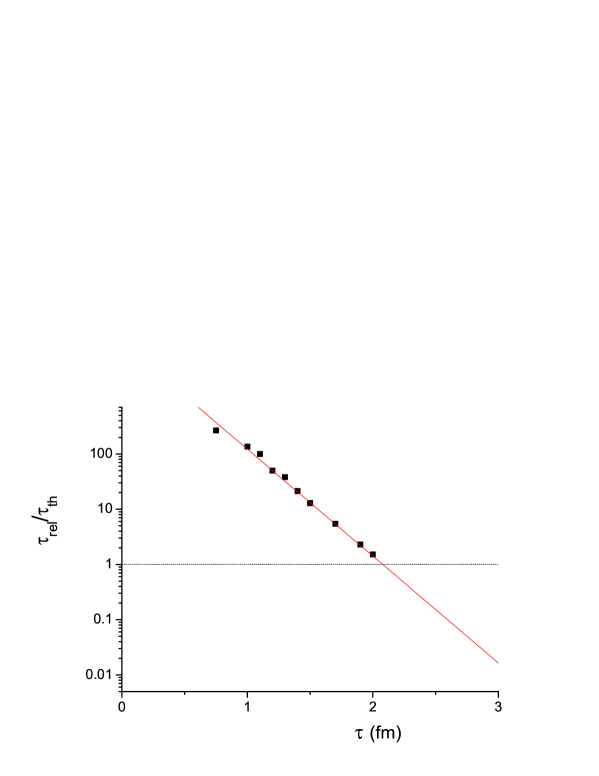
Figure 8: The dependence of the ratio $\tau_{rel}/\tau_{th}$ on the quench duration $\tau$ for $\lambda^{2}=20$. The dashed line depicts an exponential fit.

As we observe, for a wide range of $\tau$ values ($\tau\lesssim 2.1$ fm in the $\lambda^{2}=20$ case), $\tau_{rel}/\tau_{th}>1$ and especially for small $\tau$ it can be sufficiently large ($\tau_{rel}/\tau_{th}\simeq 10$ for $\tau\simeq 1.6$ fm). As the model parameter $\tau$ increases, the ratio $\tau_{rel}/\tau_{th}$ decreases almost exponentially as can be induced from the exponential fit presented with the dashed line in fig. 8.

The effect of $\lambda^{2}$ (that is the value of the $m_{\sigma}$ at $T=0$) is not so crucial and $\tau_{rel}$ shows a small decrease with decreasing $\lambda^{2}$, while $\tau_{th}$ increases slightly. However, for a given value of the interval $\tau_{rel}-\tau_{th}$ the pion production from the critical $\sigma$’s is controlled by $\lambda^{2}$. Since the $\sigma$-decay rate is larger for larger $m_{\sigma}/m_{\pi}$, we expect faster decay for $\lambda^{2}=20$ compared to $\lambda^{2}=10$, since in the former case the final $m_{\sigma}$ is larger. Experimentally we expect a larger number of produced pions in the $\lambda^{2}=20$ case. Inversely, when $\lambda^{2}=20$ a smaller interval $\tau_{rel}-\tau_{th}$ is needed in order to produce a given number of pions through the decay of critical $\sigma$’s. This is the main difference of the two $\lambda^{2}$ cases, although the corresponding plots look alike.

The discussion above reveals that the critical behavior of the $\sigma$-field will sustain, in a significant percentage of the initial configurations, for times after the $\sigma$’s start to decay, thus transferring the critical profile to the produced pions, despite the abrupt non-equilibrium evolution from its initial equilibrated state.

It is important to exclude the inverse possibility, i.e appearance of events with fractal geometry being generated out of the evolution of conventional initial conditions. Therefore, we perform the following test: We evolve our system using an ensemble of $\sigma$-configurations with random initial conditions. This conventional profile always possesses $\langle d_{f}\rangle\approx 3$ with a very small standard deviation ($\approx 0.02$). In this case not even one configuration (out of $10^{4}$) acquires slope $\lesssim 2.96$ ever, while the distribution becomes even narrower as times passes. As a consequence, $P(t)$ and $\langle P\rangle_{t}$ are always exactly equal to zero, within the used population. Therefore, the detection of events with critical profile at the freeze out, will offer safe signatures of the initial criticality of the system. The requirement $\langle P\rangle_{t}\geq 0.5\%$ remains robust for a long time and for a variety of $\lambda^{2}$ and $\tau$ as we have shown, providing a guarantee that such events are very likely to be observed in experiments of relatively high statistics.

The above treatment shows, together with other approaches in the past Antoniou2001 ; hatta03 ; SRS2 ; Randrup00 ; biro97 , that a systematic study of event-by-event fluctuations in relativistic nuclear collisions gives rise to a powerful tool in the search for novel, unconventional effects associated with QCD phase transitions (critical fluctuations, disoriented chiral condensates, dissipation at the chiral phase transition). In this work we have examined the evolution of critical fluctuations neglecting the effects of dissipation in this out-of-equilibrium process. Although a detailed study of dissipative aspects of this evolution is beyond the scope of this work, an estimate of their influence on the fractal structure of critical fluctuations is necessary before drawing our final conclusions. For this purpose we have considered a simplified modification of $\sigma$ field dynamics adding a dissipative term $\Gamma\dot{\sigma}(\vec{x},t)-\gamma\nu(t)$ in the first equation (3). $\nu(t)$ is the noise term fulfilling the relations $\langle\nu(t)\rangle=0$ and $\langle\nu(t)\nu(t^{\prime})\rangle=\gamma^{2}\delta(t-t^{\prime})$. The coefficients $\Gamma$ and $\gamma$ are related through the formula $\gamma=\sqrt{2\Gamma T/V}$, resulting from the fluctuation-dissipation theorem, with $T$ the environment temperature and $V$ the system volume. The friction coefficient $\Gamma$ introduces a new time scale in the process ($\tau_{f}=\Gamma^{-1}$) associated with the rolling down of the effective potential biro97 . With this modification we have solved the equations of motion (3) following the method discussed in the beginning of this section.

We use the typical values $\lambda^{2}=20$ and $\tau=1$ fm, and for the friction we impose $\Gamma^{-1}\simeq 0.5$ fm, which corresponds to the strong friction regime biro97 . As we observe in fig. 9, $\langle\sigma(t)\rangle$ and $\Psi(t)$ change significantly compared to the non-dissipative case, and the traces of the initial fractal geometry dilute faster.

Figure 9: $\langle\sigma\rangle$, $\psi(t)$ (solid line), $\langle\psi\rangle_{t}$ (dotted line) and $P(t)$ (solid line), $\langle P\rangle_{t}$ (dotted line), in the strong dissipative case ($\Gamma^{-1}\simeq 0.5$ fm), for $\lambda^{2}=20$ and $\tau=1$ fm.

However, the change in $\langle P\rangle_{t}$ does not spoil its observability since $\tau_{th}$ and $\tau_{rel}$ are almost unaffected (see the inset in fig. 9c). Hence, dissipation influences the mean values evolution, but it does not affect qualitatively the fluctuation-related measures such as $\langle P\rangle_{t}$. Therefore, the signals of the initial critical characteristics are still visible in the event-by-event analysis. Moreover, we have found, as expected, that weakening the dissipation, i.e decreasing $\Gamma$, its effects are suppressed and the system evolution tends smoothly to that of the non-dissipative case.

IV Summary and Conclusions

In this work we have explored the dynamics of critical fluctuations which are expected to occur in the $\sigma$-mode, near the QCD critical point. For this purpose we have adapted the $\sigma$-model Lagrangian in order to describe correctly the characteristics of the order parameter associated with the critical endpoint of the QCD phase transition RW . The issue is of primary importance in the search for the existence and location of the QCD critical point, in experiments with nuclei. At the phenomenological level these fluctuations are expressed through the fractal mass dimension of the $\sigma$-field configurations, determining the properties of the condensate at criticality Antoniou2001 . We have studied the evolution of the initial critical characteristics of the $\sigma$-field in thermal equilibrium and the possibility to reveal signals of critical fluctuations not affected by the dynamics which drives the system out-of-equilibrium. We found that for a wide range of quench time-scales ($\tau$) and coupling values ($\lambda^{2}$), the initial critical profiles may survive for a long time after the system reaches the two-pion threshold value of the sigma mass, $m_{\sigma}=2m_{\pi}$. This result is more transparent in an event-by-event study of the phenomenon, where the evolution of individual configurations is investigated.

As a consequence of this study, the fractal dimension of critical fluctuations in QCD matter, turns out to be a remarkable index for the location of the QCD critical point, in experiments with nuclei, of relatively high statistics. In fact, it remains robust, in a class of events, against dynamical effects and it leads to a characteristic pattern of intermittent fluctuations Antoniou2001 ; Bialas86 in transverse momentum space, providing us with a signature of the critical point without ambiguities owing to dynamics.

Acknowledgements:

We thank N. Tetradis for useful discussions. One of us (E.N.S) wishes to thank the Greek State Scholarship’s Foundation (IKY) for financial support. The authors acknowledge partial financial support through the research programs “Pythagoras” of the EPEAEK II (European Union and the Greek Ministry of Education) and “Kapodistrias” of the University of Athens.

References

- (1) Proceedings, RIKEN BNL Research Center Workshop, Vol. 80, BNL-75692-2006.
- (2) N. G. Antoniou et al, Letter of Intent, CERN-SPSC-2006-001.
- (3) F. Karsch, [arXiv:hep-lat/0601013]; Z. Fodor and S. Katz, JHEP 0404, 050 (2004) [arXiv:hep-lat/0402006]; R. V. Gavai and S. Gupta, Phys. Rev. D 71, 114014 (2005) [arXiv:hep-lat/0412035].
- (4) N. G. Antoniou and A. S. Kapoyannis, Phys. Lett. B 563, 165 (2003) [arXiv:hep-ph/0211392]; N. G. Antoniou, F. K. Diakonos and A. S. Kapoyannis, Nucl. Phys. A 759, 417 (2005) [arXiv:hep-ph/0503176].
- (5) A. Lesne, Renormalization Methods; Critical Phenomena; Chaos; Fractal Structures, John Wiley & Sons Ltd, (1998); P. M. Chaikin, T. C. Lubensky Principles of condensed matter physics, Cambridge University Press (1997).
- (6) N. G. Antoniou, Y. F. Contoyiannis, F. K. Diakonos, A. I. Karanikas and C. N. Ktorides , Nucl. Phys. A 693, 799 (2001) [arXiv:hep-ph/0012164]; N. G. Antoniou, Y. F. Contoyiannis, F. K. Diakonos and G. Mavromanolakis, Nucl. Phys. A 761, 149 (2005) [arXiv:hep-ph/0505185].
- (7) K. Rajagopal and F. Wilczek, [arXiv:hep-ph/0011333].
- (8) J. Berges and K. Rajagopal, Nucl. Phys. B 538, 215 (1999) [arXiv:hep-ph/9804233 ]; M. A. Stephanov, Prog. Theor. Phys. Suppl. 153, 139 (2004) [arXiv:hep-ph/0402115].
- (9) Y. Hatta and T. Ikeda, Phys. Rev. D 67, 014028 (2003) [arXiv:hep-ph/0210284]; N. G. Antoniou, F. K. Diakonos, A. S. Kapoyannis and K. S. Kousouris, Phys. Rev. Lett. 97, 032002 (2006) [arXiv:hep-ph/0602051].
- (10) H. Fujii, Phys. Rev. D 67, 094018 (2003) [arXiv:hep-ph/0302167].
- (11) M. Gell-Mann and M. Levy, Nuovo Cim. 16 (1960) 705.
- (12) K. Rajagopal and F. Wilczek, Nucl. Phys. B 399 (1993) 395 [arXiv:hep-ph/9210253].
- (13) G. Karra, R. J. Rivers, Phys. Lett. B 414, 28-33 (1997) [arXiv:hep-ph/9705243].
- (14) M. Stephanov, K. Rajagopal and E. Shuryak, Phys. Rev. D60, 114028 (1999) [hep-ph/9903292].
- (15) B. B. Mandelbrot, The Fractal Geometry of Nature, W. H. Freeman and Company, New York (1983).
- (16) T. Vicsek, Fractal Growth Phenomena, World Scientific, Singapore (1999).
- (17) K. Falconer, Fractal Geometry: Mathematical Foundations and Applications, John Wiley & Sons, West Sussex (2003).
- (18) N. G. Antoniou, Y. F. Contoyiannis, F. K. Diakonos and C. G. Papadopoulos, Phys. Rev. Lett. 81, 4289 (1998) [arXiv:hep-ph/9810383]; N. G. Antoniou, Y. F. Contoyiannis, F. K. Diakonos, Phys. Rev. E 62, 3125 (2000) [arXiv:hep-ph/0008047].
- (19) N. G. Antoniou, F. K. Diakonos, E. N. Saridakis, G. A. Tsolias, [arXiv:physics/0607038].
- (20) M. M. Tsypin, Phys. Rev. Lett. 73, 2015 (1994); J. Berges, N. Tetradis, C. Wetterich, Phys. Rep. 363, 223 (2002) [arXiv:hep-ph/0005122].
- (21) K. B. Blagoev, F. Cooper, J. F. Dawson and B. Mihaila, Phys. Rev. D 64, 125003 (2001) [arXiv:hep-ph/0106195].
- (22) N. G. Antoniou, F. K. Diakonos, E. N. Saridakis, G. A. Tsolias, [arXiv:physics/0610111].
- (23) A. Bialas and R. Peschanski, Nucl. Phys. B 273, 703 (1986); Nucl. Phys. B 308, 857 (1988).
- (24) M. Bleicher, J. Randrup, R. Snellings and X. N. Wang, Phys. Rev. C 62, 041901 (2000) [arXiv:nucl-th/0006047].
- (25) T. S. Biro and C. Greiner, Phys. Rev. Lett. 79, 3138 (1997) [arXiv:hep-ph/9704250].