Study of $K^{*}_{0}(1430)$ and $a_{0}(980)$ from $B\to K^{*}_{0}(1430)\pi$ and $B\to a_{0}(980)K$ Decays

Abstract

We use the decay modes $B\to K^{*}_{0}(1430)\pi$ and $B\to a_{0}(980)K$ to study the scalar mesons $K^{*}_{0}(1430)$ and $a_{0}(980)$ within perturbative QCD framework. For $B\to K^{*}_{0}(1430)\pi$, we perform our calculation in two scenarios of the scalar meson spectrum. The results indicate that scenario II is more favored by experimental data than scenario I. The important contribution from annihilation diagrams can enhance the branching ratios about $50\%$ in scenario I, and about $30\%$ in scenario II. The direct $CP$ asymmetries in $B\to K^{*}_{0}(1430)\pi$ are small, which are consistent with the present experiments. The predicted branching ratio of $B\to a_{0}(980)K$ in scenario I differs from the experiments by a factor 2, which indicates $a_{0}(980)$ can not be interpreted as $\bar{q}q$.

I introduction

The scalar meson spectrum is an interesting topic for both experimental and theoretical studies, but the underlying structure of the light scalar mesons is still under controversy. Many scalar meson states have been found in experiments: isoscalar states $\sigma(600)$, $f_{0}(980)$, $f_{0}(1500)$, $f_{0}(1370)$, $f_{0}(1710)$; the isovector states $a_{0}(980)$, $a_{0}(1450)$ and isodoublets $\kappa(800)$, $K^{*}_{0}(1430)$. In the literature, there are many schemes for the classification of these states scenarioI ; scalarb ; scalarc ; scalar . Here are two typical scenarios: the members of the lower mass nonet $\sigma(600)$, $\kappa(800)$, $f_{0}(980)$, and $a_{0}(980)$ are treated as the lowest lying $q\bar{q}$ states, while $K^{*}_{0}(1430)$ et al. which form the higher mass nonet are the first excited $q\bar{q}$ states; In scenario II, the members of the lower mass nonet are treated as the four-quark states scenarioI . Then the higher mass nonet is considered as the lowest lying $\bar{q}q$ states. There are also other schemes to classify these states, for example, $\sigma(600)$ and $\kappa(800)$ are not considered as the physical states, $a_{0}(980)$ (or $a_{0}(1450)$), $f_{0}(980)$, $K^{*}_{0}(1430)$ and $f_{0}(1500)$ form the $q\bar{q}$ nonet scalarc . In this paper, we study the scalar mesons in the first two scenarios.

Although intensive study has been given to the decay property of the scalar mesons, the production of these mesons can provide a different unique insight to the mysterious structure of these mesons. Compared with $D$ meson decays, the phase space in $B$ decays is larger, thus $B$ decays can provide a better place to study the scalar resonances. Experimentally, $B$ meson decay channels with a final state scalar meson have been measured in $B$ factories for several years first . Much more measurements have been reported by BaBar and Belle garmash ; babar ; belle ; abe ; new recently (see hfag for more experimental data). On the theoretical side, the $B$ decays which involve a scalar meson have been systematically studied using QCD factorization (QCDF) approach by Cheng, Chua and Yang cheng . They draw the conclusion that scenario II is more preferable. For example, in scenario I, the predicted branching ratio of $B^{-}\to\overline{K^{*}_{0}}^{0}\pi^{-}$ without annihilation is only about $1\times 10^{-5}$, which is much smaller than the experimental results. In order to explain the large data, the annihilation contribution is required to be large. But in this scenario, $a_{0}(980)$ is also a $q\bar{q}$ state and the $SU(3)$ symmetry implies a much large annihilation contribution to $B\to a_{0}(980)K$. This large annihilation contribution can lead to a larger branching ratio than the experimental upper bound. Then it is concluded that scenario I is less preferable than scenario II.

The annihilation topology contribution plays such an important role that we should pay much more attention to it. In QCD factorization approach, which is based on collinear factorization, the so-called endpoint singularity makes the annihilation contribution divergent. This might be resolved by applying the “zero-bin” subtractions which will lead to new factorization theorems in rapidity space zerobin . The more popular way to handle this divergence is the Perturbative QCD (PQCD) approach kls ; lucd . Using this approach, some pure annihilation type decays have been studied and the results are consistent with the experiments luanni , which indicates it a reliable method to deal with annihilation diagrams. In the present paper, we will use the PQCD approach to calculate the decay modes $B\to K^{*}_{0}(1430)\pi$ and $B\to a_{0}(980)K$ (in the following, we use $K^{*}_{0}$ and $a_{0}$ to denote $K^{*}_{0}(1430)$ and $a_{0}(980)$ for convenience). We will examine how large the annihilation topology contribution is, and find whether there are enough reasons to determine which scenario is more appropriate through these decay channels.

This paper is organized as follows: in the next section, we give a brief review of the scalar meson wave functions, which are important inputs in PQCD approach. What followed is the analysis of the $B\to K^{*}_{0}\pi$ and $B\to a_{0}K$ decays. The numerical results and the discussions are given in the section IV. Our conclusions are presented in the final part.

II Scalar meson distribution amplitudes

In the two-quark picture, the decay constants $f_{S}$ and $\bar{f}_{S}$ for a scalar meson $S$ are defined by:

$$\langle S(p)|\bar{q}_{2}\gamma_{\mu}q_{1}|0\rangle=f_{S}p_{\mu},\,\,\,\langle S(p)|\bar{q}_{2}q_{1}|0\rangle=\bar{f}_{S}m_{S},$$ (1)

where $m_{S}(p)$ is the mass (momentum) of the scalar meson. The vector current decay constant $f_{S}$ is zero for neutral scalar mesons $\sigma$, $f_{0}$ and $a_{0}^{0}$ due to the charge conjugation invariance or G parity conservation. In the $SU(3)$ limit, the vector decay constant of $K^{*}_{0}$ also vanishes. After including the $SU(3)$ symmetry breaking, it only gets a very small value which is proportional to the mass difference of the constituent quarks. The scalar density decay constant $\bar{f}_{S}$ can be related to the vector one by the equation of motion:

$$\mu_{S}f_{S}=\bar{f}_{S},$$ (2)

where $\mu_{S}$ is defined by $\mu_{S}=\frac{m_{S}}{m_{q_{2}}(\mu)-m_{q_{1}}(\mu)}$, which is scale dependent, thus the scalar decay constant is also scale dependent. Many model calculations have been performed for the $K^{*}_{0}$ and $a_{0}$ decayconstant . In this paper we will use the values from QCD sum rules in ref. cheng . Fixing the scale at $1\mbox{GeV}$, we specify them below:

$$\mbox{scenario}\,{\rm I}:\,\,\,\, \bar{f}_{K^{*}_{0}}=-(300\pm 30)\mbox{MeV}, f_{K^{*}_{0}}=-(25\pm 2)\mbox{MeV},$$ (3)

$$\bar{f}_{a_{0}}=(365\pm 20)\mbox{MeV};$$

$$\mbox{scenario}\,{\rm II}:\,\,\,\, \bar{f}_{K^{*}_{0}}=(445\pm 50)\mbox{MeV}, ~{}f_{K^{*}_{0}}=(37\pm 4)\mbox{MeV}.$$ (4)

Now we turn to the distribution amplitudes. The scalar meson’s light-cone distribution amplitude is defined by:

$$\langle S(p)|\bar{q}_{1\beta}(z)q_{2\alpha}(0)|0\rangle = \frac{1}{\sqrt{6}}\int^{1}_{0}dxe^{ixp\cdot z}\bigg{\{}p\!\!\!/\phi_{S}(x)+m_{S}\phi^{S}_{S}(x)-\frac{1}{6}m_{S}\sigma_{\mu\nu}p^{\mu}z^{\nu}\phi^{\sigma}_{S}(x)\bigg{\}}_{\alpha\beta}$$ (5)

$$= \frac{1}{\sqrt{6}}\int^{1}_{0}dxe^{ixp\cdot z}\bigg{\{}p\!\!\!/\phi_{S}(x)+m_{S}\phi^{S}_{S}(x)+m_{S}(n\!\!\!/\bar{n}\!\!\!/-1)\phi^{T}_{S}(x)\bigg{\}}_{\alpha\beta},$$

where $n=(1,0,0_{T})$ and $\bar{n}=(0,1,0_{T})$ are dimensionless vectors on the light cone, and $n$ is parallel with the moving direction of the scalar meson. The distribution amplitudes $\phi_{S}(x)$, $\phi^{S}_{S}(x)$ and $\phi^{\sigma}_{S}(x)$ are normalized as:

$$\int^{1}_{0}dx\phi_{S}(x)=\frac{f_{S}}{2\sqrt{6}},\,\,\,\,\,\,\int^{1}_{0}dx\phi^{S}_{S}(x)=\int^{1}_{0}dx\phi^{\sigma}_{S}(x)=\frac{\bar{f}_{S}}{2\sqrt{6}},$$ (6)

and $\phi^{T}_{S}(x)=\frac{1}{6}\frac{d}{dx}\phi^{\sigma}_{S}(x)$.

In general, the twist-2 light cone distribution amplitude $\phi_{S}(x)$ can be expanded as:

$$\phi_{S}(x,\mu) = \frac{\bar{f}_{S}(\mu)}{2\sqrt{6}}6x(1-x)\bigg{[}B_{0}(\mu)+\sum\limits^{\infty}_{m=1}B_{m}(\mu)C_{m}^{3/2}(2x-1)\bigg{]}$$ (7)

$$= \frac{{f}_{S}(\mu)}{2\sqrt{6}}6x(1-x)\bigg{[}1+\mu_{S}\sum\limits^{\infty}_{m=1}B_{m}(\mu)C_{m}^{3/2}(2x-1)\bigg{]},$$

where $B_{m}(\mu)$ and $C_{m}^{3/2}(x)$ are the Gegenbauer moments and Gegenbauer polynomials respectively. The Gegenbauer moments $B_{1}$, $B_{3}$ of distribution amplitudes for $K^{*}_{0}$ and $a_{0}$ have been calculated in cheng as

$$\mbox{scenario}\,{\rm I}:\,\,\,\,B_{1}=0.58\pm 0.07,\;\;\;\;B_{3}=-1.20\pm 0.08;$$ (8)

$$B_{1}=-0.93\pm 0.10,\;\;\;\;B_{3}=0.14\pm 0.08;$$ (9)

$$\mbox{scenario}\,{\rm II}:\,\,\,\,B_{1}=-0.57\pm 0.13,\;\;\;\;B_{3}=-0.42\pm 0.22,$$ (10)

where the second line is for $a_{0}$, and the others are for $K^{*}_{0}$. These values are also taken at $\mu=\mbox{1GeV}$.

As for the twist-3 light-cone distribution amplitudes, there is no study on their explicit Gegenbauer moments so far, so we take the asymptotic form in our numerical calculation:

$$\phi^{S}_{S}(x)=\frac{\bar{f}_{S}}{2\sqrt{6}},\,\,\,\,\,\phi^{T}_{S}(x)=\frac{\bar{f}_{S}}{2\sqrt{6}}(1-2x).$$ (11)

In our calculation, we will choose the momentum fraction on the anti-quark, thus we should use $\phi_{S}(1-x)$, $\phi^{S}_{S}(1-x)=\phi^{S}(x)$ and $\phi_{S}^{T}(1-x)=-\phi_{S}^{T}(x)$. But in the amplitudes, for simplicity, we use $\phi_{S}(x)$ to denote $\phi_{S}(1-x)$ . It is similar for the pseudoscalar meson.

III The perturbative QCD calculation

In this section we will give the decay amplitudes for the $B\to K^{*}_{0}\pi$ and $B\to a_{0}K$ decays in the PQCD approach. The PQCD approach is based on the $k_{T}$ factorization botts , where we keep the transverse momentum of the partons in a meson. In this approach there is no divergence when the longitudinal parton momentum fraction falls into the endpoint region. The weak decay matrix element can be completely factorized review :

$${\cal A}=\phi_{B}\otimes H^{(6)}\otimes J\otimes S\otimes\phi_{M_{1}}\otimes\phi_{M_{2}},$$ (12)

where $\phi_{B}$, $\phi_{M_{1}}$ and $\phi_{M_{2}}$ denote the wave functions of the $B$ meson and the light mesons, respectively. $S$ and $J$ denote the Sudakov form factor and the jet function respectively. The Sudakov form factor comes from $k_{T}$ resummation which kills the end-point singularities. The jet function is from threshold resummation which can organize the large double logarithms in the hard kernel. The symbol $\otimes$ denotes convolution of the parton longitudinal momentum fractions and the transverse momentum. $H^{(6)}$ is the six-quark hard scattering kernel, which consists of the effective four quark operators and a hard gluon to connect the spectator quark in the decay. The standard four-quark operators describing the $b\to s$ transition are defined as buras :

• current–current tree operators

  $$O_{1}=({\bar{u}}_{\alpha}b_{\beta})_{V-A}({\bar{s}}_{\beta}u_{\alpha})_{V-A},\ \ \ \ \ \ \ \ \ O_{2}=({\bar{u}}_{\alpha}b_{\alpha})_{V-A}({\bar{s}}_{\beta}u_{\beta})_{V-A},$$ (13)

• QCD penguin operators

  $$O_{3}=({\bar{s}}_{\alpha}b_{\alpha})_{V-A}\sum\limits_{q^{\prime}}({\bar{q}}^{\prime}_{\beta}q^{\prime}_{\beta})_{V-A},\ \ \ \ \ \ \ \ \ O_{4}=({\bar{s}}_{\beta}b_{\alpha})_{V-A}\sum\limits_{q^{\prime}}({\bar{q}}^{\prime}_{\alpha}q^{\prime}_{\beta})_{V-A},$$ (14)

  $$\!\!\!\!\!\!\!\!\!\!\!\!\!\!\!\!\!\!\!\!\!\!\!\!O_{5}=({\bar{s}}_{\alpha}b_{\alpha})_{V-A}\sum\limits_{q^{\prime}}({\bar{q}}^{\prime}_{\beta}q^{\prime}_{\beta})_{V+A},\ \ \ \ \ \ \ \ \ O_{6}=({\bar{s}}_{\beta}b_{\alpha})_{V-A}\sum\limits_{q^{\prime}}({\bar{q}}^{\prime}_{\alpha}q^{\prime}_{\beta})_{V+A},$$ (15)

• electro-weak penguin operators

  $$O_{7}=\frac{3}{2}({\bar{s}}_{\alpha}b_{\alpha})_{V-A}\sum\limits_{q^{\prime}}e_{q^{\prime}}({\bar{q}}^{\prime}_{\beta}q^{\prime}_{\beta})_{V+A},\ \ \ \ O_{8}=\frac{3}{2}({\bar{s}}_{\beta}b_{\alpha})_{V-A}\sum\limits_{q^{\prime}}e_{q^{\prime}}({\bar{q}}^{\prime}_{\alpha}q^{\prime}_{\beta})_{V+A},$$ (16)

  $$O_{9}=\frac{3}{2}({\bar{s}}_{\alpha}b_{\alpha})_{V-A}\sum\limits_{q^{\prime}}e_{q^{\prime}}({\bar{q}}^{\prime}_{\beta}q^{\prime}_{\beta})_{V-A},\ \ \ \ O_{10}=\frac{3}{2}({\bar{s}}_{\beta}b_{\alpha})_{V-A}\sum\limits_{q^{\prime}}e_{q^{\prime}}({\bar{q}}^{\prime}_{\alpha}q^{\prime}_{\beta})_{V-A},$$ (17)

where $q^{\prime}=(u,d,s,c,b)$. The 10 operators together with their QCD-corrected Wilson coefficients form the effective Hamiltonian:

$${\cal H}_{eff} = \frac{G_{F}}{\sqrt{2}}\left\{V_{ub}V_{us}^{*}\Big{[}C_{1}({\mu})O_{1}({\mu})+C_{2}({\mu})O_{2}({\mu})\Big{]}-V_{tb}V_{ts}^{*}{\sum\limits_{i=3}^{10}}C_{i}({\mu})O_{i}({\mu})\right\}.$$ (18)

The partition of the perturbative and non-perturbative region (factorization scale) is quite arbitrary, but the full amplitude should be independent of the partition. We usually take the largest virtuality of internal particles as the factorization scale, which is of order $\sqrt{m_{B}\Lambda}$. The leading order Wilson coefficients will be evolved to this scale. As the factorization scale in PQCD approach is smaller than the factorization scale of QCDF, which is about $m_{B}$, a large enhancement of the Wilson coefficients occurs, especially for the penguin operators kls ; lucd .

III.1 $B\to K^{*}_{0}\pi$ decays

The leading order Feynman diagrams for these decays in PQCD approach are given in Fig. -1019. The decay amplitude for each diagram can be obtained by contracting the hard scattering kernels and the meson’s wave functions. According to the power counting in PQCD approach lipc , the first two emission diagrams in Fig. -1019 give the dominant contribution. For the $(V-A)(V-A)$ kind of operators, the decay amplitudes for these two diagrams are given by:

$$F^{L}_{B\to\pi}(a) = \frac{32\pi}{3}m_{B}^{4}f_{K^{*}_{0}}\int_{0}^{1}dx_{1}dx_{3}\int_{0}^{\infty}b_{1}db_{1}\,b_{3}db_{3}\,\phi_{B}(x_{1},b_{1})\bigg{\{}a(t)E_{e}(t)$$ (19)

$$\times\left[(1+x_{3})\phi_{\pi}^{A}(x_{3})+r_{\pi}(1-2x_{3})\left(\phi_{\pi}^{P}(x_{3})+\phi_{\pi}^{T}(x_{3})\right)\right]h_{e}(x_{1},x_{3},b_{1},b_{3})$$

$$\;\;\;\;\;\;+2r_{\pi}\phi_{\pi}^{P}({x_{3}})a(t^{\prime})E_{e}(t^{\prime})h_{e}(x_{3},x_{1},b_{3},b_{1})\bigg{\}},$$

where $r_{\pi}=m_{0}^{\pi}/m_{B}$, $m_{0}^{\pi}$ is the chiral enhancement scale and $a$ is the corresponding Wilson coefficient. $E_{e}(t)$ is defined as

$$E_{e}(t) = \alpha_{s}(t)\exp[-S_{B}(t)-S_{\pi}(t)].$$ (20)

For the $(V-A)(V+A)$ kind of operators, the decay amplitudes for these two diagrams are given by:

$$F^{R}_{B\to\pi}(a) = -\frac{64\pi}{3}m_{B}^{4}r_{K^{*}_{0}}{\overline{f_{K^{*}_{0}}}}\int_{0}^{1}dx_{1}dx_{3}\int_{0}^{\infty}b_{1}db_{1}\,b_{3}db_{3}\,\phi_{B}(x_{1},b_{1})\bigg{\{}a(t)E_{e}(t)$$ (21)

$$\times\left[\phi_{\pi}^{A}(x_{3})+r_{\pi}x_{3}\left(\phi_{\pi}^{P}(x_{3})-\phi_{\pi}^{T}(x_{3})\right)+2r_{\pi}\phi_{\pi}^{P}(x_{2})\right]h_{e}(x_{1},x_{3},b_{1},b_{3})$$

$$\;\;\;\;\;\;+2r_{\pi}\phi_{2}^{P}(x_{3})a(t^{\prime})E_{e}(t^{\prime})h_{e}(x_{3},x_{1},b_{3},b_{1})\bigg{\}}\;,$$

with the factorization scales $t=\max{\{\sqrt{x_{3}}m_{B},1/b_{1},1/b_{3}\}}$ and $t^{\prime}=\max{\{\sqrt{x_{1}}m_{B},1/b_{1},1/b_{3}\}}$, $r_{K^{*}_{0}}=m_{K^{*}_{0}}/m_{B}$. The Sudakov form factors $S_{B}(t)$ and $S_{\pi}(t)$ and the hard functions $h_{e}$ and others like $h_{a}$, $h_{na}$ are given explicitly in ref.kls ; lucd .

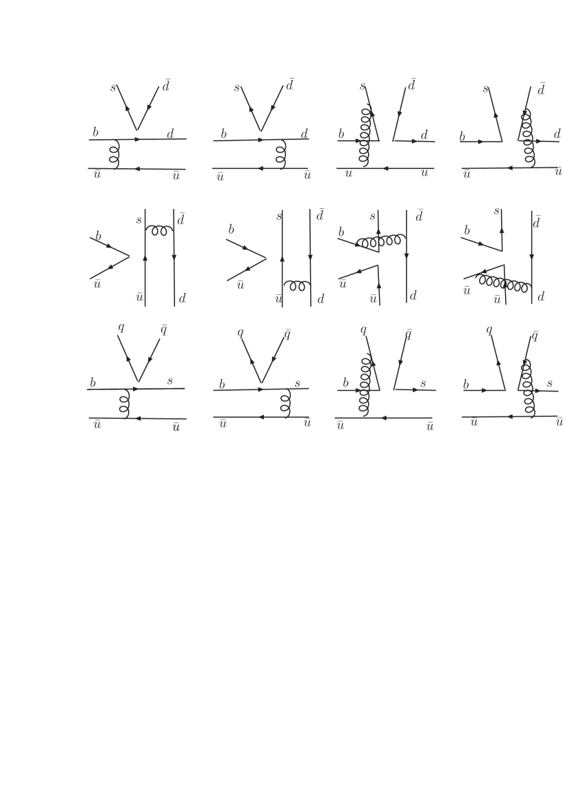
Figure -1019: The leading order Feynman diagrams in PQCD for $B\to K^{*}_{0}\pi$ and $B\to a_{0}K$

Comparing $F^{L}_{B\to\pi}$ and $F^{R}_{B\to\pi}$, we find that the first one is proportional to the small vector decay constant, but the latter is proportional to the scalar decay constant which is strongly chiral enhanced, so $F^{R}_{B\to\pi}$ will give the dominant contribution.

In ref. cheng , the author found that the vertex corrections and hard-spectator-scattering corrections can enhance $a_{4}$ sizably. In PQCD approach, the vertex corrections are at the next-to-leading order in $\alpha_{s}$, so we neglect it in our calculation, but we include the hard spectator scattering (the last two diagrams in the first row of Fig. -1019). After the calculation, the non-factorization decay amplitudes for the $(V-A)(V-A)$ kind of operators read:

$${\cal M}^{L}_{B\to\pi}(a) = \frac{128\pi}{3\sqrt{6}}m_{B}^{4}\int_{0}^{1}dx_{1}dx_{2}dx_{3}\int_{0}^{\infty}b_{1}db_{1}\,b_{2}db_{2}\,\phi_{B}(x_{1},b_{1})\phi_{K^{*}_{0}}(x_{2})$$ (22)

$$\times\bigg{\{}-\Big{[}(x_{2}-1)\phi_{\pi}(x_{3})+r_{\pi}x_{3}\left(\phi_{\pi}^{P}(x_{3})-\phi_{\pi}^{T}(x_{3})\right)\Big{]}a(t)E^{\prime}_{e}(t)h_{n}(x_{1},1-x_{2},x_{3},b_{1},b_{2})$$

$$-\Big{[}(x_{2}+x_{3})\phi_{\pi}(x_{3})-r_{\pi}x_{3}\left(\phi_{\pi}^{P}(x_{3})+\phi_{\pi}^{T}(x_{3})\right)\Big{]}a(t^{\prime})E^{\prime}_{e}(t^{\prime})h_{n}(x_{1},x_{2},x_{3},b_{1},b_{2})\bigg{\}}.$$

For the $(V-A)(V+A)$ kind of operators, the decay amplitudes for these two diagrams are given by:

$${\cal M}^{R}_{B\to\pi}(a) = \frac{128\pi}{3\sqrt{6}}m_{B}^{4}r_{K^{*}_{0}}\int_{0}^{1}dx_{1}dx_{2}dx_{3}\int_{0}^{\infty}b_{1}db_{1}\,b_{2}db_{2}\,\phi_{B}(x_{1},b_{1})\bigg{\{}a(t)E^{\prime}_{e}(t)\times$$ (23)

$$\left[(x_{2}-1)\left(\phi_{\pi}^{A}(x_{3})(\phi_{K^{*}_{0}}^{S}(x_{2})+\phi_{K^{*}_{0}}^{T}(x_{2}))\right.+r_{\pi}(\phi_{\pi}^{P}(x_{3})-\phi_{\pi}^{T}(x_{3}))(\phi_{K^{*}_{0}}^{S}(x_{2})+\phi_{K^{*}_{0}}^{T}(x_{2}))\right)$$

$$\;\;\;\;\;\left.-r_{\pi}x_{3}\left(\phi_{\pi}^{P}(x_{3})+\phi_{\pi}^{T}(x_{3})\right)\left(\phi_{K^{*}_{0}}^{S}(x_{2})-\phi_{K^{*}_{0}}^{T}(x_{2})\right)\right]h_{n}(x_{1},1-x_{2},x_{3},b_{1},b_{2})+$$

$$\left[x_{2}\phi_{\pi}^{A}(x_{3})\left(\phi_{K^{*}_{0}}^{S}(x_{2})-\phi_{K^{*}_{0}}^{T}(x_{2})\right)\right.+r_{\pi}x_{2}\left(\phi_{\pi}^{P}(x_{3})-\phi_{\pi}^{T}(x_{3})\right)\left(\phi_{K^{*}_{0}}^{S}(x_{2})-\phi_{K^{*}_{0}}^{T}(x_{2})\right)$$

$$\left.+r_{\pi}x_{3}\left(\phi_{\pi}^{P}(x_{3})+\phi_{\pi}^{T}(x_{3})\right)\left(\phi_{K^{*}_{0}}^{S}(x_{2})+\phi_{K^{*}_{0}}^{T}(x_{2})\right)\right]a(t^{\prime})E^{\prime}_{e}(t^{\prime})h_{n}(x_{1},x_{2},x_{3},b_{1},b_{2})\bigg{\}},$$

where $E^{\prime}_{e}(t)=\alpha_{s}(t)\exp[-S_{B}(t)-S_{2}(t)-S_{3}(t)]$, the factorization scales are chosen by

$$t = \max{\{\sqrt{x_{1}x_{3}}m_{B},\sqrt{|(1-x_{1}-x_{2})x_{3}|}m_{B},1/b_{1},1/b_{2}\}},$$ (24)

$$t^{\prime} = \max{\{\sqrt{x_{1}x_{3}}m_{B},\sqrt{|(x_{1}-x_{2})x_{3}|}m_{B},1/b_{1},1/b_{2}\}}.$$ (25)

From the above formulae, we can see that the two hard spectator scattering diagrams contribute constructively for ${\cal M}^{L}_{B\to\pi}$ while most contributions cancelled for ${\cal M}^{R}_{B\to\pi}$. So it is expected that the $(V-A)(V-A)$ kind operator contribution can give an important contribution as in $B\to f_{0}K$ f0K . However, these diagrams are suppressed compared with the factorizable ones for a smaller Wilson coefficient $C_{3}$, thus they cannot play such an important role as in QCDF cheng .

In PQCD approach, the annihilation type diagrams are free of endpoint singularity, so they can be calculated systematically. The Feynman diagrams are plotted in the second row of Fig. -1019. For the first two factorizable annihilation diagrams, the decay amplitude formulae are written as:

$$F^{L}_{a}(a) = \frac{32\pi}{3}m_{B}^{4}f_{B}\int_{0}^{1}dx_{2}dx_{3}\int_{0}^{\infty}b_{2}db_{2}\,b_{3}db_{3}\$$ (26)

$$\times\Bigg{\{}\Big{[}(x_{3}-1)\phi_{\pi}^{A}(x_{3})\phi_{K^{*}_{0}}(x_{2})-2r_{\pi}r_{K^{*}_{0}}(x_{3}-2)\phi_{\pi}^{P}(x_{3})\phi_{K^{*}_{0}}^{S}(x_{2})$$

$$~{}~{}+2r_{\pi}r_{K^{*}_{0}}x_{3}\phi_{K^{*}_{0}}^{S}(x_{2})\phi_{\pi}^{T}(x_{3})\Big{]}a(t)E_{a}(t)h_{a}(x_{2},1-x_{3},b_{2},b_{3})$$

$$+\Big{[}x_{2}\phi_{\pi}^{A}(x_{3})\phi_{K^{*}_{0}}(x_{2})-2r_{\pi}r_{K^{*}_{0}}\phi_{\pi}^{P}(x_{3})((x_{2}+1)\phi_{K^{*}_{0}}^{S}(x_{2})+(x_{2}-1)\phi_{K^{*}_{0}}^{T}(x_{2}))\Big{]}$$

$$\,\,\,\times a(t^{\prime})E_{a}(t^{\prime})h_{a}(1-x_{3},x_{2},b_{3},b_{2})\Bigg{\}},$$

for the $(V-A)(V-A)$ kind of operators and

$$F^{R}_{a}(a) = -\frac{64\pi}{3}m_{B}^{4}f_{B}\int_{0}^{1}dx_{2}dx_{3}\int_{0}^{\infty}b_{2}db_{2}\,b_{3}db_{3}\,\Bigg{\{}E_{a}(t)a(t)h_{a}(x_{2},1-x_{3},b_{2},b_{3})$$ (27)

$$\times\Big{[}r_{\pi}(x_{3}-1)\phi_{K^{*}_{0}}(x_{2})\left(\phi_{\pi}^{P}(x_{3})+\phi_{\pi}^{T}(x_{3})\right)+2r_{K^{*}_{0}}\phi_{\pi}(x_{3})\phi_{K^{*}_{0}}^{S}(x_{2})\Big{]}$$

$$-\Big{[}2r_{\pi}\phi_{K^{*}_{0}}(x_{2})\phi_{\pi}^{P}(x_{3})+r_{K^{*}_{0}}x_{2}\phi_{\pi}(x_{3})\left(\phi_{K^{*}_{0}}^{T}(x_{2})-\phi_{K^{*}_{0}}^{S}(x_{2})\right)\Big{]}$$

$$\times a(t^{\prime})E_{a}(t^{\prime})h_{a}(1-x_{3},x_{2},b_{3},b_{2})\Bigg{\}},$$

for the $(V-A)(V+A)$ kind of operators, where

$$E_{a}(t) = \alpha_{s}(t)\exp[-S_{2}(t)-S_{3}(t)],$$ (28)

with $t=\max{\{\sqrt{1-x_{3}}m_{B},1/b_{2},1/b_{3}\}}$ and $t^{\prime}=\max{\{\sqrt{x_{2}}m_{B},1/b_{2},1/b_{3}\}}$.

For the non-factorizable annihilation diagrams, e.g., the last two diagrams in the second row of Fig. 1, the factorization formulae read:

$${\cal M}^{L}_{a}(a) = \frac{128\pi}{3\sqrt{6}}m_{B}^{4}\int_{0}^{1}dx_{1}dx_{2}dx_{3}\int_{0}^{\infty}b_{1}db_{1}\,b_{2}db_{2}\,\phi_{B}(x_{1},b_{1})\bigg{\{}\left[-x_{2}\phi_{\pi}^{A}(x_{3})\phi_{K^{*}_{0}}(x_{2})\right.$$ (29)

$$\;\;\;\;\;\;+r_{\pi}r_{K^{*}_{0}}\phi_{\pi}^{P}(x_{3})\left((x_{2}-x_{3}+3)\phi_{K^{*}_{0}}^{S}(x_{2})+(x_{2}+x_{3}-1)\phi_{K^{*}_{0}}^{T}(x_{2})\right)$$

$$\;\;\;\;\;\;\left.+r_{\pi}r_{K^{*}_{0}}\phi_{\pi}^{T}(x_{3})\left((1-x_{2}-x_{3})\phi_{K^{*}_{0}}^{S}(x_{2})+(1-x_{2}+x_{3})\phi_{K^{*}_{0}}^{T}(x_{2})\right)\right]$$

$$\,\,\,\,\,\,\,\;\;\times a(t)E^{\prime}_{e}(t)h_{na}(x_{1},x_{2},x_{3},b_{1},b_{2})-\left[(x_{3}-1)\phi_{\pi}^{A}(x_{3})\phi_{K^{*}_{0}}(x_{2})\right.$$

$$\;\;\;\;\;\;+r_{\pi}r_{K^{*}_{0}}\phi_{\pi}^{P}(x_{3})\left((x_{2}-x_{3}+1)\phi_{K^{*}_{0}}^{S}(x_{2})-(x_{2}+x_{3}-1)\phi_{K^{*}_{0}}^{T}(x_{2})\right)$$

$$\;\;\;\;\;\;\left.+r_{\pi}r_{K^{*}_{0}}\phi_{\pi}^{T}(x_{3})\left((x_{2}+x_{3}-1)\phi_{K^{*}_{0}}^{S}(x_{2})-(1+x_{2}-x_{3})\phi_{K^{*}_{0}}^{T}(x_{2})\right)\right]$$

$$\,\,\,\,\,\,\,\,\,\times a(t^{\prime})E^{\prime}_{e}(t^{\prime})h^{\prime}_{na}(x_{1},x_{2},x_{3},b_{1},b_{2})\bigg{\}}\;,$$

and for the $(V-A)(V-A)$ kind of operators

$${\cal M}^{R}_{a}(a) = \frac{128\pi}{3\sqrt{6}}m_{B}^{4}\int_{0}^{1}dx_{1}dx_{2}dx_{3}\int_{0}^{\infty}b_{1}db_{1}\,b_{2}db_{2}\,\phi_{B}(x_{1},b_{1})\times$$ (30)

$$\bigg{\{}\left[r_{\pi}(x_{3}-1)\phi_{K^{*}_{0}}(x_{2})(\phi_{\pi}^{T}(x_{3})-\phi_{\pi}^{P}(x_{3}))+r_{K^{*}_{0}}x_{2}\phi_{\pi}(x_{3})(\phi_{K^{*}_{0}}^{S}(x_{2})+\phi_{K^{*}_{0}}^{T}(x_{2}))\right]$$

$$\;\;\times a(t)E^{\prime}_{e}(t)h_{na}(x_{1},x_{2},x_{3},b_{1},b_{2})$$

$$-\left[r_{\pi}(x_{3}-1)\phi_{K^{*}_{0}}(x_{2})(\phi_{\pi}^{T}(x_{3})-\phi_{\pi}^{P}(x_{3}))+r_{K^{*}_{0}}x_{2}\phi_{\pi}(x_{3})(\phi_{K^{*}_{0}}^{S}(x_{2})+\phi_{K^{*}_{0}}^{T}(x_{2}))\right]$$

$$\;\;\times a(t^{\prime})E^{\prime}_{e}(t^{\prime})h^{\prime}_{na}(x_{1},x_{2},x_{3},b_{1},b_{2})\bigg{\}}\;,$$

for the $(V-A)(V+A)$ kind of operators, where

$$t = \max{\{\sqrt{x_{2}(1-x_{3})}m_{B},\sqrt{1-(1-x_{1}-x_{2})x_{3}}m_{B},1/b_{1},1/b_{2}\}},$$

$$t^{\prime} = \max{\{\sqrt{x_{2}(1-x_{3})m_{B}},\sqrt{|(x_{1}-x_{2})(1-x_{3})|}m_{B},1/b_{1},1/b_{2}\}}.$$

Summing up all contributions mentioned above, the decay amplitude for $B\to\overline{K^{*}_{0}}^{0}\pi^{-}$ is

$$A(B^{-}\to\overline{K^{*}_{0}}^{0}\pi^{-}) =\frac{G_{F}}{\sqrt{2}}\bigg{[}V_{ub}V_{us}^{*}\bigg{\{}F^{L}_{a}(a_{1})+{\cal M}^{L}_{a}(C_{1})\bigg{\}}$$ (31)

$$-V_{tb}V_{ts}^{*}\bigg{\{}F^{L}_{e}(a_{4}-\frac{1}{2}a_{10})+F^{R}_{e}(a_{6}-\frac{1}{2}a_{8})+F^{L}_{a}(a_{4}+a_{10})+F^{R}_{a}(a_{6}+a_{8})$$

$$\;\;+{\cal M}^{L}_{e}(C_{3}-\frac{1}{2}C_{9})+{\cal M}^{R}_{e}(C_{5}-\frac{1}{2}C_{7})+{\cal M}^{L}_{a}(C_{3}-\frac{1}{2}C_{9})+{\cal M}^{R}_{a}(C_{5}-\frac{1}{2}C_{7})\bigg{\}}\bigg{]},$$

where the combinations of Wilson coefficients are defined as usual akl :

$$a_{1}=C_{2}+C_{1}/3, a_{3}=C_{3}+C_{4}/3,~{}a_{5}=C_{5}+C_{6}/3,~{}a_{7}=C_{7}+C_{8}/3,~{}a_{9}=C_{9}+C_{10}/3,$$ (32)

$$a_{2}=C_{1}+C_{2}/3, a_{4}=C_{4}+C_{3}/3,~{}a_{6}=C_{6}+C_{5}/3,~{}a_{8}=C_{8}+C_{7}/3,~{}a_{10}=C_{10}+C_{9}/3.$$ (33)

For the decays $\bar{B}^{0}\to K_{0}^{*-}\pi^{+}$, $B^{-}\to K_{0}^{*-}\pi^{0}$ and $\bar{B}^{0}\to\overline{K^{*}_{0}}^{0}\pi^{0}$, the analysis is similar, except the last two channels include the $\pi$-emission diagrams in the third row of Fig. -1019. The decay amplitudes of the factorizable $\pi$-emission diagrams for the $(V-A)(V-A)$ kind of operators are written by:

$$F^{L}_{B\to K^{*}_{0}}(a) = \frac{32\pi}{3}m_{B}^{4}f_{\pi}\int_{0}^{1}dx_{1}dx_{2}\int_{0}^{\infty}b_{1}db_{1}\,b_{2}db_{2}\,\phi_{B}(x_{1},b_{1})\bigg{\{}a(t)E_{e}(t)$$ (34)

$$\times\left[(1+x_{2})\phi_{K^{*}_{0}}(x_{2})-r_{K^{*}_{0}}(1-2x_{2})\left(\phi_{K^{*}_{0}}^{s}(x_{2})+\phi_{K^{*}_{0}}^{T}(x_{2})\right)\right]h_{e}(x_{1},x_{2},b_{1},b_{2})$$

$$\;\;\;\;\;\;-2r_{K^{*}_{0}}\phi_{K^{*}_{0}}^{s}({x_{2}})a(t^{\prime})E_{e}(t^{\prime})h_{e}(x_{2},x_{1},b_{2},b_{1})\bigg{\}},$$

and for the $(V-A)(V+A)$ kind of operators:

$$F^{R}_{B\to K^{*}_{0}}(a)=-F^{L}_{B\to K^{*}_{0}}(a).$$ (35)

For the non-factorizable diagrams $(V-A)(V-A)$ operators:

$${\cal M}^{L}_{B\to K^{*}_{0}}(a) = \frac{128\pi}{3\sqrt{6}}m_{B}^{4}\int_{0}^{1}dx_{1}dx_{2}dx_{3}\int_{0}^{\infty}b_{1}db_{1}\,b_{3}db_{3}\,\phi_{B}(x_{1},b_{1})\phi_{\pi}^{A}(x_{3})\bigg{\{}a(t)E^{\prime}_{e}(t)$$ (36)

$$\bigg{[}(1-x_{3})\phi_{K^{*}_{0}}(x_{2})+r_{K^{*}_{0}}x_{2}\bigg{(}\phi_{K^{*}_{0}}^{s}(x_{2})-\phi_{K^{*}_{0}}^{T}(x_{2})\bigg{)}\bigg{]}h_{n}(x_{1},1-x_{3},x_{2},b_{1},b_{3})$$

$$+\left[-(x_{2}+x_{3})\phi_{K^{*}_{0}}(x_{2})-r_{K^{*}_{0}}x_{2}(\phi_{K^{*}_{0}}^{s}(x_{2})+\phi_{K^{*}_{0}}^{T}(x_{2}))\right]$$

$$a(t^{\prime})E^{\prime}_{e}(t^{\prime})h_{n}(x_{1},x_{3},x_{2},b_{1},b_{3})\bigg{\}}\;,$$

and for $(V-A)(V+A)$ operators

$${\cal M}^{R}_{B\to K^{*}_{0}}(a) = \frac{128\pi}{3\sqrt{6}}m_{B}^{4}\int_{0}^{1}dx_{1}dx_{2}dx_{3}\int_{0}^{\infty}b_{1}db_{1}\,b_{3}db_{3}\,\phi_{B}(x_{1},b_{1})\phi_{\pi}^{A}(x_{3})\bigg{\{}-a(t)E^{\prime}_{e}(t)$$ (37)

$$\bigg{[}(x_{2}-x_{3}+1)\phi_{K^{*}_{0}}(x_{2})+r_{K^{*}_{0}}x_{2}(\phi_{K^{*}_{0}}^{s}(x_{2})+\phi_{K^{*}_{0}}^{T}(x_{2}))\bigg{]}h_{n}(x_{1},1-x_{3},x_{2},b_{1},b_{3})$$

$$+\left[x_{3}\phi_{K^{*}_{0}}(x_{2})+r_{K^{*}_{0}}x_{2}(\phi_{K^{*}_{0}}^{s}(x_{2})-\phi_{K^{*}_{0}}^{T}(x_{2}))\right]a(t^{\prime})E^{\prime}_{e}(t^{\prime})h_{n}(x_{1},x_{3},x_{2},b_{1},b_{3})\bigg{\}}\;.$$

We write the decay amplitudes for the other three channels below:

$$A(\bar{B}^{0}\to K_{0}^{*-}\pi^{+}) =\frac{G_{F}}{\sqrt{2}}\Big{[}V_{ub}V_{us}^{*}\left\{F^{L}_{B\to\pi}(a_{1})+{\cal M}^{L}_{B\to\pi}(C_{1})\right\}$$ (38)

$$-V_{tb}V_{ts}^{*}\Big{\{}F^{L}_{B\to\pi}(a_{4}+a_{10})+F^{R}_{B\to\pi}(a_{6}+a_{8})+F^{L}_{a}(a_{4}-\frac{1}{2}a_{10})+F^{R}_{a}(a_{6}-\frac{1}{2}a_{8})$$

$$\;\;\;\;+{\cal M}^{L}_{B\to\pi}(C_{3}+C_{9})+{\cal M}^{R}_{B\to\pi}(C_{5}+C_{7})+{\cal M}^{L}_{a}(C_{3}-\frac{1}{2}C_{9})+{\cal M}^{R}_{a}(C_{5}-\frac{1}{2}C_{7})\Big{\}}\Big{]},$$

$$A(B^{-}\to K_{0}^{*-}\pi^{0}) =\frac{G_{F}}{{2}}\Big{[}V_{ub}V_{us}^{*}\left\{F^{L}_{B\to\pi}(a_{1})+{\cal M}^{L}_{B\to\pi}(C_{1})+F^{L}_{B\to K^{*}_{0}}(a_{2})+{\cal M}^{L}_{B\to K^{*}_{0}}(C_{2})+F^{L}_{a}(a_{1})+{\cal M}^{L}_{a}(C_{1})\right\}$$ (39)

$$-V_{tb}V_{ts}^{*}\Big{\{}F^{L}_{B\to\pi}(a_{4}+a_{10})+F^{R}_{B\to\pi}(a_{6}+a_{8})+F^{L}_{B\to K^{*}_{0}}(\frac{3}{2}a_{9}-\frac{3}{2}a_{7})$$

$$\;\;\;+F^{L}_{a}(a_{4}+a_{10})+F^{R}_{a}(a_{6}+a_{8})$$

$$\;\;\;+{\cal M}^{L}_{B\to\pi}(C_{3}+C_{9})+{\cal M}^{R}_{B\to\pi}(C_{5}+C_{7})+{\cal M}^{L}_{B\to K^{*}_{0}}(\frac{3}{2}C_{10})+{\cal M}^{R}_{B\to K^{*}_{0}}(\frac{3}{2}C_{8})$$

$$\;\;\;+{\cal M}^{L}_{a}(C_{3}+C_{10})+{\cal M}^{R}_{a}(C_{5}+C_{7})\Big{\}}\Big{]},$$

$$A(\bar{B}^{0}\to\overline{K^{*}_{0}}^{0}\pi^{0}) =\frac{G_{F}}{{2}}\Big{[}V_{ub}V_{us}^{*}\left\{F^{L}_{B\to K^{*}_{0}}(a_{2})+{\cal M}^{L}_{B\to K^{*}_{0}}(C_{2})\right\}$$ (41)

$$\;\;\;-V_{tb}V_{ts}^{*}\Big{\{}-F^{L}_{B\to\pi}(a_{4}-\frac{1}{2}a_{10})-F^{R}_{B\to\pi}(a_{6}-\frac{1}{2}a_{8})+F^{L}_{B\to K^{*}_{0}}(\frac{3}{2}a_{9})+F^{R}_{B\to K^{*}_{0}}(\frac{3}{2}a_{7})$$

$$\;\;\;\;-F^{L}_{a}(a_{4}-\frac{1}{2}a_{10})-F^{R}_{a}(a_{6}-\frac{1}{2}a_{8})$$

$$\;\;\;-{\cal M}^{L}_{B\to\pi}(C_{3}-\frac{1}{2}C_{9})-{\cal M}^{R}_{B\to\pi}(C_{5}-\frac{1}{2}C_{7})+{\cal M}^{L}_{B\to K^{*}_{0}}(\frac{3}{2}C_{10})+{\cal M}^{R}_{B\to K^{*}_{0}}(\frac{3}{2}C_{8})$$

$$\;\;\;-{\cal M}^{L}_{a}(C_{3}-\frac{1}{2}C_{9})-{\cal M}^{R}_{a}(C_{5}-\frac{1}{2}C_{7})\Big{\}}\Big{]}.$$

The isospin relation for the four channels holds exactly in these equations:

$$\sqrt{2}A(\bar{B}^{0}\to\overline{K^{*}_{0}}^{0}\pi^{0})+A(\bar{B}^{0}\to K_{0}^{*-}\pi^{+})=\sqrt{2}A(B^{-}\to K_{0}^{*-}\pi^{0})-A(B^{-}\to\overline{K^{*}_{0}}^{0}\pi^{-}).$$ (42)

III.2 $B\to a_{0}K$ decays

As mentioned above, the predicted branching fractions of $B\to a_{0}K$, which overshoot the experimental limits, are regarded as an evidence to rule out scenario I in QCDF, thus it is important to see whether it is the same in the PQCD approach.

The Feynman diagrams for these decays are completely the same as the $B\to K^{*}_{0}\pi$ except that we should identify the $s\bar{q}$ and $q\bar{q}$ as $K$ and $a_{0}$ rather than $K^{*}_{0}$ and $\pi$, then each channel corresponds to the one in $B\to K^{*}_{0}\pi$. Their factorization formulae can be derived from the corresponding channels directly. The $K$-emission and annihilation decay amplitudes of $B\to a_{0}K$ can be obtained from $B\to K^{*}_{0}\pi$ by making the substitution:

$$\phi_{K^{*}_{0}}\to\phi^{A}_{K},\phi^{S}_{K^{*}_{0}}\to\phi^{P}_{K},\phi^{T}_{K^{*}_{0}}\to\phi^{T}_{K},$$

$$\phi^{A}_{\pi}\to\phi_{a_{0}},\phi^{P}_{\pi}\to-\phi^{S}_{a_{0}},\phi^{T}_{\pi}\to-\phi^{T}_{a_{0}}.$$ (43)

The $a_{0}$-emission diagrams have only nonfactorizable contributions, the substitution for $(V-A)(V-A)$ operators is:

$$\phi^{A}_{\pi}\to\phi_{a_{0}},\phi^{P}_{\pi}\to\phi^{S}_{a_{0}},\phi^{T}_{\pi}\to\phi^{T}_{a_{0}},$$ (44)

$$\phi_{K^{*}_{0}}\to\phi^{A}_{K},\phi^{S}_{K^{*}_{0}}\to-\phi^{P}_{K},\phi^{T}_{K^{*}_{0}}\to-\phi^{T}_{K},$$

but for $(V-A)(V+A)$ operators,

$$\phi^{A}_{\pi}\to\phi_{a_{0}},\phi^{P}_{\pi}\to\phi^{S}_{a_{0}},\phi^{T}_{\pi}\to\phi^{T}_{a_{0}},$$ (46)

$$\phi_{K^{*}_{0}}\to-\phi^{A}_{K},\phi^{S}_{K^{*}_{0}}\to\phi^{P}_{K},\phi^{T}_{K^{*}_{0}}\to\phi^{T}_{K}.$$

Compared with $B\to K^{*}_{0}\pi$, the features of $B\to a_{0}K$ are:

• For the decays $\bar{B^{0}}\to a_{0}^{+}K^{-}$ and $B^{-}\to a_{0}^{-}\bar{K}^{0}$, the emitted particle is $K$, which can be produced through the axial-vector current without any suppression, thus the operator $O_{4}$ can give a large contribution to the emission factorizable amplitudes. But this term has a minus sign relative to $O_{6}$, so the penguin operators cancel with each other sizably. The contribution from tree operators can be large due to the large Wilson coefficients $a_{1}$ in $B^{-}\to a_{0}^{+}K^{-}$.

• In $B\to\overline{K^{*}_{0}}^{0}\pi^{-}$, the emitted particle ($\overline{K^{*}_{0}}^{0}$) is a scalar meson, the two hard spectator scattering diagrams (non-factorizable) can enhance each other due to the anti-symmetric twist-2 distribution amplitudes. But in $\bar{B^{0}}\to a_{0}^{+}K^{-}$ and $B^{-}\to a_{0}^{-}\bar{K}^{0}$, the emitted particle is a pseudoscalar, there are cancellations between the two hard spectator scattering diagrams. So the hard spectator scattering contribution is rather small.

• The annihilation diagrams of the four $B\to a_{0}K$ channels are similar with each other, the dominant contributions are all from the $S\to P$ time-like form factor mediated by an $(S+P)$ density.

• $\bar{B^{0}}\to a_{0}^{0}\bar{K}^{0}$ and $B^{-}\to a_{0}^{0}K^{-}$ are more complicated due to the appearance of the $a_{0}$-emission diagrams. Because of the vanishing vector decay constant of $a_{0}$, the factorizable emission diagrams are zero. For the nonfactorizable diagrams, the QCD penguin operators cancel for the neutral state of isospin triplet. The electroweak penguin operators have a small Wilson coefficients, thus the emission contributions in these channels are small. For the tree operators, although they are suppressed by the CKM matrix elements, the nonfactorizable emission diagrams can be enhanced for the large Wilson coefficients $C_{2}$. So it is expected a large CP asymmetry in the decays $\bar{B^{0}}\to a^{0}_{0}\bar{K}^{0}$ and $B^{-}\to a^{0}_{0}K^{-}$.

From the above discussion, we can see that the dominant contributions are from the annihilation diagrams and the diagrams with tree operators.

IV Results and discussions

Table 1: Input parameters used in the numerical calculation

Masses	$m_{K^{*}_{0}}=1.412\mbox{ GeV}$,	$m_{0}^{K}=1.7\mbox{ GeV}$,	$m_{0}^{\pi}=1.4\mbox{ GeV}$
	$m_{a_{0}}=0.98{\mbox{ GeV}}$	$M_{B}=5.28\mbox{ GeV}$
Decay constants	$f_{B}=0.19\mbox{ GeV}$	$f_{K}=0.16\mbox{ GeV}$	$f_{\pi}=0.132\mbox{ GeV}$
Life Times	$\tau_{B^{\pm}}=1.671\times 10^{-12}\mbox{ s}$	$\tau_{B^{0}}=1.536\times 10^{-12}\mbox{ s}$
CKM	$V_{tb}=0.9997$	$V_{ts}=-0.04$,
	$V_{us}=0.2196$	$V_{ub}=0.00367e^{-i60^{\circ}}$

For numerical calculations, we have employed the parameters in Tab. 1. For the $B$ meson wave function, we adopt the Gaussian-type model kls (we choose the shape parameter $\omega=0.4$). As for the light-cone distribution amplitudes (LCDAs) of the pion and kaon, we use the results from QCD sum rules up to twist-3 QCDSR . Other parameters relevant to the scalar mesons have been given in the second section.

IV.1 The Branching Ratios and The CP Asymmetries

Table 2: Various decay amplitudes ($\times 10^{-2}\mbox{GeV}^{3}$) in decay $B^{-}\to\overline{K^{*}_{0}}^{0}\pi^{-}$ and $B^{-}\to a_{0}^{-}\bar{K}^{0}$

	$F^{L}_{e}(a_{4})$	$F^{R}_{e}(a_{6})$	${\cal M}^{L}_{e}(C_{3})+M_{e}^{R}(C_{5})$	$F^{L}_{a}(a_{4})+F_{a}^{R}(a_{6})+{\cal M}_{a}^{L}(C_{3})+{\cal M}_{a}^{R}(C_{5})$	$F^{L}_{a}(a_{2})+{\cal M}^{L}_{a}(C_{1})$
scenario I	$0.98$	$-12$	$0.78+1.2i$	$7.4+13.3i$	$8.8-11.8i$
scenario II	$-1.4$	$17.9$	$2.1-0.37i$	$-5.8-17.8i$	$-13.6-0.11i$
$B^{-}\to a_{0}^{-}\bar{K}^{0}$	$9.3$	$-11.3$	$0.09-0.74i$	$2.0-9.0i$	$8.6+1.2i$

Using the parameters in the above, we give the numerical results for different amplitudes of $B^{-}\to\bar{K}^{*0}_{0}\pi^{-}$ in Table 2. The numerical results confirm that the emission diagram of $(V-A)(V-A)$ operators $F_{B\to\pi}^{L}(a_{4})$ indeed give small contributions because of the small vector current decay constant. The $(V-A)(V+A)$ operators give the dominant contribution $F_{e}^{R}(a_{6})$. The opposite sign between scenario I and scenario II comes from the decay constant of the $K^{*}_{0}$ meson. The non-factorizable contribution ${\cal M}^{L}_{B\to\pi}(C_{3})$ is small due to the small Wilson coefficient. ${\cal M}^{R}_{B\to\pi}(C_{5})$ is even smaller because of the cancellation between the two diagrams.

According to PQCD power counting, the annihilation diagrams are power suppressed, but the suppression is not so effective in some cases, such as when chiral enhancement existing. Usually there is a large imaginary part in the amplitudes of the annihilation diagrams, which is the source of strong phase in PQCD approach. The numerical results in Table 2 indicate that the annihilation diagrams in scenario I are more important than that in scenario II. There are also tree operators contributing to the annihilation diagrams $F^{L}_{a}(a_{2})+{\cal M}^{L}_{a}(C_{1})$, which are Cabibbo suppressed, but they are essential in direct $CP$ violation.

Table 3: Branching ratios for the decays $B\to K^{*}_{0}\pi$ and $B\to a_{0}K$(in units of $10^{-6}$). The first theoretical error is from the decay constant of the scalar meson, the second and the third one is Gengebauer moments $B_{1}$ and $B_{3}$, the uncertainty caused the CKM angle $\gamma$ is very small which is not listed here. The experimental data listed here are the world average values by the Heavy Flavor Averaging Group (HFAG) hfag .

Channel	scenario I	scenario II	exp.	Channel	scenario I	exp.
$B^{-}\to\overline{K^{*}_{0}}^{0}\pi^{-}$	$20.7^{+4.3+0.8+1.8}_{-3.9-0.8-1.6}$	$47.6^{+11.3+3.7+6.9}_{-10.1-3.6-5.1}$	$41.2\pm 4.2$	$B^{-}\to\bar{K}^{0}a_{0}^{-}$	$6.9^{+0.8+1.1+2.0}_{-0.7-1.1-1.7}$	$<3.9$
$\bar{B}^{0}\to K^{*-}_{0}\pi^{+}$	$20.0^{+4.2+0.8+1.6}_{-3.8-0.7-1.5}$	$43.0^{+10.2+3.1+7.0}_{-9.1-2.9-5.2}$	$46.6^{+5.6}_{-6.6}$	$\bar{B}^{0}\to K^{-}a_{0}^{+}$	$9.7^{+1.1+1.6+2.7}_{-1.0-1.4-2.2}$	$<1.6$
$\bar{B}^{0}\to\overline{K^{*}_{0}}^{0}\pi^{0}$	$10.0^{+2.1+0.4+1.0}_{-1.9-0.5-0.9}$	$18.4^{+4.4+1.5+4.0}_{-3.9-1.4-2.9}$	$25.5\pm 9.9$	$\bar{B}^{0}\to\bar{K}^{0}a_{0}^{0}$	$4.7^{+0.5+0.7+1.1}_{-0.5-0.8-1.1}$	$<7.8$
$B^{-}\to K^{*-}_{0}\pi^{0}$	$11.3^{+2.4+0.4+0.7}_{-2.1-0.3-0.7}$	$28.8^{+6.8+1.9+3.2}_{-6.1-1.9-3.5}$	-	$B^{-}\to K^{-}a_{0}^{0}$	$3.5^{+0.4+0.4+1.0}_{-0.4-0.6-1.0}$	$<2.5$

Now it is straightforward to obtain the results for the $CP$-averaged branching ratio of $B^{-}\to\bar{K}^{*0}_{0}\pi^{-}$, which is given in Tab. 3. Comparing the two scenarios, we find: the results from scenario II are twice as scenario I, the most important reason is the larger scalar decay constant in scenario II; secondly, the nonfactorizable diagrams are small, they only change the branching ratio slightly; the annihilation diagrams play an important role in both scenarios, it can enhance the branching ratios about $50\%$ in scenario I, and about $30\%$ in scenario II. The current experimental data hfag is also listed in Tab. 3. The large branching ratio is consistent with the results in scenario II, so scenario II is more preferable than scenario I, this conclusion is consistent with cheng . But the difference with cheng is: we directly calculate the annihilation contribution in $B\to K^{*}_{0}\pi$, rather than fit the $B\to K^{*}_{0}\pi$ data and then use the $B\to a_{0}K$ data to rule out scenario I.

The decay amplitudes for the $B^{-}\to a_{0}^{-}\bar{K^{0}}$ decay are also listed in table 2, the results indicate that the emission diagrams almost cancelled out, as expected in section III. The branching ratio is dominated by the annihilation diagrams which is at the same level as the $B^{-}\to\overline{K^{*}_{0}}^{0}\pi^{-}$, and the induced branching ratio is about twice larger than the experimental upper bound. The results also show that scenario I is not supported by the current experimental data.

In the above discussion, we concentrate on $B^{-}\to\overline{K^{*}_{0}}^{0}\pi^{-}$ and $B\to a_{0}^{-}\bar{K^{0}}$. The dominant contribution in $B\to K^{*}_{0}\pi$ for other channels is the same with $B^{-}\to\overline{K^{*}_{0}}^{0}\pi^{-}$ by isospin symmetry, except the contribution from the electro-weak penguin and the tree operators which can violate isospin symmetry. To explore the deviation of the isospin limit, it is convenient to define the parameters below:

$$R_{1}=\frac{{\cal B}({\bar{B}^{0}\to{K^{*0}_{0}}\pi^{0}})}{{\cal B}({\bar{B}^{0}\to K^{*-}_{0}\pi^{+}})},$$

$$R_{2}=\frac{{\cal B}({B^{-}\to K^{*-}_{0}\pi^{0}})}{{\cal B}({B^{-}\to{K^{*0}_{0}}\pi^{-}})},$$

$$R_{3}=\frac{\tau(B^{0})}{\tau(B^{-})}\frac{{\cal B}({B^{-}\to{K^{*0}_{0}}\pi^{-}})}{{\cal B}({\bar{B}^{0}\to K^{*-}_{0}\pi^{+}})}.$$ (48)

For $B\to a_{0}K$, the definition is the similar except $K^{*}_{0}\to K,\pi\to a_{0}$. These parameters are the ratios of the branching fractions, which should be less sensitive to many nonperturbative inputs than the branching fractions, thus it is more persuadable to test these parameters. In the isospin limit, if we ignore the $CKM$ suppressed tree diagrams and electro-weak penguins, $R_{1}$, $R_{2}$ and $R_{3}$ should be equal to 0.5, 0.5 and 1.0. The deviations reflect the magnitude of the tree operators and the electro-weak penguins directly. Our results and the experimental data are given in table 4, where we use the central values in table 3 for the experiment data. In both scenarios, the deviations from isospin limit are not large, which shows that the QCD penguin are dominant in the branching ratios, both in emission diagrams and the annihilation diagrams. The three ratios for $B\to a_{0}K$ decays are: $R_{1}=0.48,R_{2}=0.51,R_{3}=0.68$. There is a large deviation for the ratio $R_{3}$, and the reason is the large tree contribution. So the large direct CP asymmetry for $B^{0}\to a^{-}_{0}K^{+}$ is also expected.

Table 4: Ratios of the branching fractions in $B\to K^{*}_{0}\pi$. For the experimental values, we only use the central values.

Ratios	isospin limit	Scenario II	Scenario I	Experiment
$R_{1}$	0.5	0.43	0.48	0.39
$R_{2}$	0.5	0.61	0.55	-
$R_{3}$	1.0	1.02	0.95	0.81

The contribution from different effective operators shown in Eqs. (31-41) have been categorized to two groups according to the different $CKM$ matrix elements:

$$\bar{A}=\frac{G_{F}}{\sqrt{2}}[V_{ub}V_{us}^{*}T-V_{tb}V_{ts}^{*}P],$$ (49)

where $T/P$ denotes the amplitude which comes from the tree/penguin operators respectively. The charge conjugate channel decay amplitude is the same as Eq. (49) except the sign of the weak phase. The formula for the direct CP asymmetry reads:

$$A_{CP}=\frac{|\bar{A}|^{2}-|A|^{2}}{|\bar{A}|^{2}-|A|^{2}}=\frac{2z\sin{\gamma}\sin{\delta}}{1-2z\cos{\gamma}\cos{\delta}+z^{2}},$$ (50)

where $z=|\frac{V_{tb}V_{ts}^{*}}{V_{ub}V_{us}^{*}}||\frac{P}{T}|$, $\delta$ is the relative strong phase between two groups of contributions. This equation indicates that the direct $CP$ violation depends on the ratio of the tree and penguin contribution. The direct $CP$ asymmetry is very small if the ratio is too large or too small, while the comparable tree and penguin contributions imply large direct $CP$ asymmetries. For $B\to K^{*}_{0}\pi$, the penguin operators give the dominant contribution, but the tree operators suffer from the $CKM$ suppression, so it is expected the direct $CP$ asymmetry is small. We list our results in table 5 as well as the experimental data hfag , where the results are consistent with the experiments in both scenarios. But in the decay $B^{0}\to a_{0}K$, as mentioned above, the emission penguin contribution cancels, while the tree operators are large, sizable direct $CP$ asymmetries are predicted in these channels, especially in $\bar{B^{0}}\to a_{0}^{+}K^{-}$ and $B^{-}\to a_{0}^{0}K^{-}$. In QCDF, the central values of direct $CP$ asymmetries for all four channels are very small, but with large uncertainties for $B^{-}\to a_{0}^{0}K^{-}$ and $\bar{B}^{0}\to a_{0}^{+}K^{-}$. Furthermore, we may expect the similar size of $CP$ asymmetries in similar decays $B\to a_{0}(1450)K$.

Table 5: Direct CP asymmetries (in units of %)

Channel	Scenario I	Scenario II	exp.	channels	$A_{CP}$
$B^{-}\to\overline{K^{*}_{0}}^{0}\pi^{-}$	$-1.5$	$-1.7$	$-5^{+5}_{-8}$	$B^{-}\to\bar{K}^{0}a_{0}^{-}$	4
$\bar{B}^{0}\to K^{*-}_{0}\pi^{+}$	$9.2$	$0.22$	$-7\pm 14$	$\bar{B}^{0}\to K^{-}a_{0}^{+}$	-70
$\bar{B}^{0}\to\overline{K^{*}_{0}}^{0}\pi^{0}$	$-9.0$	$-6.8$	$-34\pm 19$	$\bar{B}^{0}\to\bar{K}^{0}a_{0}^{0}$	-17
$B^{-}\to K^{*-}_{0}\pi^{0}$	$16.0$	$3.5$	-	$B^{-}\to K^{-}a_{0}^{0}$	-70

IV.2 The Theoretical Uncertainties

In the above calculation, the uncertainties from the decay constants can give sizable effects on the branching ratio, but not to the direct $CP$ asymmetries. Furthermore, there are other sources of uncertainties:

• The twist-3 distribution amplitudes of the scalar mesons are taken as the asymptotic form for lack of more reasonable results from non-perturbative methods. These distribution amplitudes will be studied in the future work LWZ . In LWZ , we find the Gegenbauer moments of the twist-3 distribution amplitudes are rather small, which implies the results will not be changed sizably.

• The Gegenbauer moments $B_{1}$ and $B_{3}$ for twist-2 LCDAs of $K^{*}_{0}$ and $a_{0}$ have sizable uncertainties, which can lead to the theoretical errors. We include these uncertainties in the results and they can give about $20\%\sim 30\%$ uncertainties to the branching ratio.

• The uncertainties of the light pseudoscalar meson and $B$ meson wave functions, the factorization scale, et al. have been studied extensively in kurimoto . The uncertainty from the factorization scale is within $10\%$. The major source of the uncertainty comes from the meson distribution amplitudes. The results can be varied by $(10-30)\%$ by changing the parameter in the wave functions.

• The sub-leading order contributions in PQCD approach have also been neglected in this calculation, but these corrections have been calculated in refs. subleadingPQCD for $B\to\pi K,\pi\pi$, etc. These corrections can change the penguin dominated processes about $20\%$ of the branching ratio of $B\to\pi K$. We may expect similar effect in $B\to K^{*}_{0}\pi$.

• The uncertainties of $CKM$ matrix elements and the $CKM$ phase angle can also affect the branching ratios and $CP$ asymmetries. In the two kinds of decays considered in this paper, the decay amplitudes are the functions of the $CKM$ angle $\gamma$, whose value given in PDG06 is $\gamma=(63^{+15}_{-12})^{\circ}$ pdg06 . With the $CKM$ angle $\gamma$ varying at this area, we find that the error area is very small in $B\to K^{*}_{0}\pi$ decays in both scenarios. For the $B\to a_{0}K$ decays, the error area is some larger, but within ten percent.

• The long distance re-scattering can also affect the branching ratios and $CP$ asymmetries. This effect could be phenomenologically studied in the final-state interactions FSI . We need more data to determine whether it is necessary to include the re-scattering effect in $B\to SP$ decays.

V summary

In this paper, we calculate the decay modes $B\to K^{*}_{0}\pi$ and $B\to a_{0}K$ within perturbative QCD framework. For $B\to K^{*}_{0}\pi$, we perform our calculation in two scenarios of the scalar meson spectrum, our calculation indicates that: scenario II is more consistent with the experimental data than scenario I. We directly calculate the contribution from annihilation diagrams: it can enhance the branching ratios about $50\%$ in scenario I, and about $30\%$ in scenario II. Our predicted branching ratio of $B\to a_{0}K$ in scenario I is larger than the experimental upper bound, which indicates $a_{0}(980)$ can not be interpreted as $\bar{q}q$. We calculated the direct $CP$ asymmetries and the isospin parameters in these decays, and we find that in $B\to K^{*}_{0}\pi$ (in both scenarios) the direct $CP$ asymmetries are small, which are consistent with the present experiments; the deviation from the isospin limit is also small. There is large $CP$ asymmetries in $B\to a_{0}(980)K$ due to the relatively large tree contributions in scenario I. We expect similar $CP$ asymmetries in $B\to a_{0}(1450)K$ .

References

• (1) G.L. Jaffe, Phys. Rev. D15, 267(1977); $ibid$: 15, 281(1977); S.G. Gorishinii, A.L. Kataev and S.A. Larin, Phys. Lett. B135,457(1984); N.N. Achasov, Phys. Usp. 41, 1149(1998), Usp. Fiz. Nauk 168, 1257 (1998),arXiv: hep-ph/9904223; A.L. Kataev, Phys. Atom. Nucl. 68, 567 (2005), Yad. Fiz. 68, 597(2005), arXiv: hep-ph/0406305; A. Vijande, A. Valcarce, F. Fernandez and B. Silvestre-Brac, Phys. Rev. D72, 034025(2005).
• (2) V. Elias, A.H. Fariborz, F. Shi, T.G. Steele, Nucl. Phys. A 633, 279(1998); E. van Beveren, Eur. Phys. J.C10, 469(1999); D. Black, A.H. Fariborz and J. Schechter, Phys. Rev D61, 074001(2000); E. van Beveren, Phys. Lett. B495, 300(2000); Erratum-ibid. B509, 365(2001); F. Kleefeld, E. van Beveren and M.D. Scadron, Phys. Rev. D66, 034007(2002); M. Ishida and S. Ishida, arXiv: hep-ph/0310062; M.D. Scadron, G. Rupp, F. Kleefeld and E. van Beveren, Phys. Rev. D69, 014010(2004); Erratum-ibid.D69, 059901(2004); A.M. Fariborz, Int. J. Mod. Phys. A19, 2095(2004); Int. J. Mod. Phys. A19, 5417(2004); Phys. Rev. D74, 054030(2006); S. Narison, Phys. Rev. D73, 114024(2006); E. van Beveren, D.V. Bugg, F. Kleefeld and G. Rupp, Phys. Lett. B641, 265(2006).
• (3) P. Minkowski and W. Ochs, Euro. Phys. J. C9, 283(1999).
• (4) S. Spanier and N. A. TΓΆrnqvist, β€œNote on scalar mesons” in Particle Data Group, Journal of Physics G 33, 1(2006); S.Godfrey and J. Napolitano, Rev. Mod. Phys. 71,1411(1999); F. E. Close and N. A. TΓΆrnqvist, J. Phys. G 28, R249(2002).
• (5) Belle Collaboraion, K. Abe et al., Phys. Rev. D65, 092005(2002).
• (6) Belle Collaboraion, A. Garmash et al., Phys. Rev.D71, 092003(2005); Belle Collabaraion, A. Garmash et al., arXiv: hep-ex/0505048.
• (7) Babar Collaboration, B. Aubert et al., Phys. Rev. D70, 092001(2004); Phys. Rev. D70, 111102 (2004); Phys. Rev. D72, 072003(2005); arXiv: hep-ex/0408032, hep-ex/0408073.
• (8) Belle Collaboration, K. Abe et al., arXiv: hep-ex/0509047; Belle Collaboration, A. Bonder et al., arXiv: hep-ex/0411004.
• (9) Belle Collaboration, K. Abe et al., hep-ex/0509001.
• (10) Babar Collaboration, B. Aubert et al., Phys. Rev. D74, 032003(2006); hep-ex/0607112.
• (11) Heavy Flavor Averaging Group, P. Chang, et al., http://www.slac.stanford.edu/xorg/hfag.
• (12) H.-Y. Cheng, C.-K. Chua, K.-C. Yang, Phys. Rev. D73, 014017(2006).
• (13) A.V. Manohar and I.W. Stewart, arXiv: hep-ph/0607001.
• (14) Y.Β Y.Β Keum, H.-n. Li and A.Β I.Β Sanda, Phys. Lett. B504, 6(2001); Phys. Rev. D63, 054008 (2001); C.H. Chen, Y.Y. Keum and H.-n. Li, Phys. Rev. D66, 054013(2002).
• (15) C.-D. LΓΌ, K. Ukai, M.-Z. Yang, Phys. Rev. D63, 074009 (2001); C.Β D.Β LΓΌ and M.Β Z.Β Yang, Eur. Phys. J. C23, 275(2002).
• (16) C. D. LΓΌ, K. Ukai, Eur. Phys. J. C28, 305 (2003); Y. Li, C. D. LΓΌ, J. Phys. G29, 2115 (2003); High Energy Phys. Nucl. Phys. 27, 1062(2003).
• (17) T.V. Brito, F.S. Navarra, M. Nielsen, and M.E. Fracco, Phys. Lett. B608, 69(2005); K. Maltman, Phys. Lett. B462, 14(1999); S. Narison, Nucl. Phys. Proc. Suppl. 86, 242(2000); C.M. Shakin and H.S. Wang, Phys. Rev. D63, 074017(2001); D.S. Du, J.W. Li and M.Z. Yang, Phys. Lett.B 619, 105(2005).
• (18) J. Botts and G. Sterman, Nucl. Phys. B325, 62 (1989).
• (19) H.N. Li, Prog. Part. Nucl. Phys. 51, 85(2003).
• (20) For a review, see G. Buchalla, A.J. Buras, M.E. Lautenbacher, Rev. Mod. Phys. 68, 1125(1996).
• (21) C.H. Chen, Y.Y. Keum and H.-n. Li, Phys. Rev. D64, 112002(2003).
• (22) W. Wang, Y.L. Shen, Y. Li and C.D. LΓΌ, arXiv: hep-ph/0609082.
• (23) A. Ali, G. Kramer, C.D. LΓΌ, Phys. Rev. D58, 094009 (1998)
• (24) V. M. Braun, I. E. Fliyakov, Z. Phys. C48, 239(1990); P. Ball, JHEP, 9901, 010(1999); V.M. Braun and A. Lenz, Phys. Rev. D70, 074020 (2004); P. Ball and R. Zwicky, Phys. Lett B 633, 289(2006); P. Ball, V.M. Braun and A. Lenz, JHEP 0605, 004(2006).
• (25) C.D. LΓΌ, Y.M. Wang and H. Zou, hep-ph/0612210.
• (26) T. Kurimoto, Phys. Rev. D74, 014027(2006).
• (27) H.N. Li, S. Mishima and A.I. Sanda, Phys. Rev. D72, 114005(2005); H.N. Li and S. Mishima, ibid: 73,114014(2006); arXiv: hep-ph/0608277.
• (28) Particle data group, Journal of Physics G 33, 1 (2006).
• (29) H.Y. Cheng, C.K. Chua and A. Soni, Phys. Rev. D71, 014030(2005); C.D. LΓΌ, Y.L. Shen and W. Wang, Phys. Rev. D73, 034005(2006).