hep-ph/0610375 ANL-PR-06-69 EFI-06-19 Baryogenesis
from an Earlier Phase Transition

Abstract

We explore the possibility that the observed baryon asymmetry of the universe is the result of an earlier phase transition in which an extended gauge sector breaks down into the $SU(3)_{C}\times SU(2)_{L}\times U(1)_{Y}$ of the Standard Model. Our proto-typical example is the Topflavor model, in which there is a separate $SU(2)_{1}$ for the third generation from the $SU(2)_{2}$ felt by the first two generations. We show that the breakdown of $SU(2)_{1}\times SU(2)_{2}\rightarrow SU(2)_{L}$ results in lepton number being asymmetrically distributed through-out the three families, and provided the SM electroweak phase transition is not strongly first order, results in a non-zero baryon number, which for parameter choices that can be explored at the LHC, may explain the observed baryon asymmetry.

1 Introduction

The origin of the observed baryon asymmetry of the universe is one of the most fundamental open questions in particle physics and cosmology. Numerically, the baryon-to-entropy ratio is

$$\eta_{B}\equiv\frac{n_{B}}{s}=9.2^{+0.6}_{-0.4}\times 10^{-11}\,,$$ (1)

where $n_{B}=n_{b}-n_{\bar{b}}$ and $s$ are the baryon number density and entropy, respectively. Famously, Sakharov has shown [1] that in order to generate a baryon asymmetry in an initially baryon-symmetric universe, there must be: (1) baryon number ($B$) violation; (2) $C$ and $CP$ violation; and (3) a departure from thermal equilibrium. These requirements, especially in light of null results obtained by experimental searches for $B$-violation (for example, proton decay), are difficult to realize in the framework of an electroweak (EW) scale model, prompting attention to high scale mechanisms such as GUT baryogenesis [2, 3, 4, 5], leptogenesis [6, 7] and the Affleck-Dine scenario [8]. Such mechanisms can be viable, but are difficult to test experimentally.

However, the Standard Model (SM) already contains a way to reconcile large baryon-number violation at the EW scale with the lack of experimental evidence for such interactions at low scales. As noted by Kuzmin, Rubakov and Shaposhnikov [9], the baryon-number violation induced by sphaleron transitions between two different $N$-vacua of the $SU(2)_{L}$ electroweak interaction are unsuppressed at temperatures larger than the EW scale, but are so highly suppressed at low energies as to be essentially irrelevant. This idea of electroweak baryogenesis (EWBG) [10] is very attractive, and could have been realized within the SM. EWBG makes very specific demands of the electroweak symmetry-breaking (EWSB) sector of the theory, and leads to observable consequences at future colliders. For example, the need for $B$-violating interactions to be out of equilibrium at the time of the phase transition requires that the electroweak phase transition is strongly first order, with

$$\frac{\langle\phi(T_{c})\rangle}{T_{c}} \gtrsim 1~{}.$$ (2)

This in turn puts constraints on the Higgs potential, and demands a small Higgs quartic (and hence Higgs mass).

Electroweak baryogenesis in the SM is thus ruled out; the LEP-II bound on the SM Higgs mass [11], $m_{h}^{SM}\gtrsim 115$ GeV is incompatible with a the requirement that the sphaleron processes be out of equilibrium at the phase transition, Eq (2). While this renders the SM itself unable to produce the asymmetry, it illustrates the fact that experiments at the TeV scale are able to directly probe EWBG. Extensions of the SM which include new physics at the EW scale can in fact re-open the possibility of EW baryogenesis by introducing additional bosonic fields [12, 13, 14, 15, 16] as in the Minimal Supersymmetric Standard Model (MSSM) [17, 18, 19, 20, 21, 22, 23, 24] or fermions strongly coupled to the Higgs [31, 32]. Eventually, future colliders such as the Large Hardron Collider (LHC) and possibly International Linear Collider (ILC) will unravel the nature of EWSB, and should provide a better understanding as to the nature of the electroweak phase transition (EWPT). If it proves first order, this will be a crucial piece of indirect evidence for EWBG. If it does not, it will raise the interesting question: Does the idea of electroweak baryogenesis have to be abandoned?

While the lack of a first order EWPT would strongly disfavor electroweak baryogenesis, it may be that the basic picture of baryon-number violating processes arising from non-perturbative gauge theory dynamics, impotent at low energies but unsuppressed at the TeV scale, can survive. Since many extensions of the SM predict the existence of new non-Abelian gauge symmetries at the TeV scale, it may be that some theories already addressing unrelated problems may in fact contain the ingredients necessary for “electro-weak style” baryogenesis. A new gauge group $G$ could break down somewhere above the EWPT, and generate an asymmetry through its own strongly first order phase transition.

This is a novel idea, but one which is not entirely straight-forward to realize in a realistic setting. Below this new phase transition, the theory is still $SU(2)_{L}\times U(1)_{Y}$ symmetric, and the usual EW sphalerons are unsuppressed. They will try to wash-out any generated baryon asymmetry unless $B-L\neq 0$. In principle, one could arrange the representations of the SM matter under the new gauge symmetry $G$ such that $B-L$ is not preserved due to the nonzero mixed anomaly $G$-$G$-$U(1)_{B-L}$, but this kind of non-universal assignment of representations is also somewhat delicate. The requirement that $G$-$G$-$U(1)_{Y}$ gauge anomalies cancel will in general require more chiral fermions charged under $G$ and the SM. Thus, we will not consider this possibility in detail. Instead, we employ a more subtle mechanism in which $G$ acts only on the third generation fermions, and thus $B-L$ is conserved (within a generation). The breakdown of $G$ can thus be accompanied by production of an asymmetry among the third family quarks and leptons. Baryon number will quickly equilibriate among the three families because of the large quark masses and mixings, but each lepton family number will remain distinct because of the tiny neutrino masses. Above the EWPT, the EW sphalerons will result in $B=0$ and $L_{1}=L_{2}=-L_{3}/2\neq 0$. Provided the EW sphalerons are in equilibrium during the EWPT, as the fermion masses turn on from EW symmetry-breaking, a non-zero (though diluted) baryon number will result [33, 34]. So in fact this mechanism requires that the EWPT not be strongly first order.

The outline of this paper is as follows. In Section 2, we review how a baryon asymmetry can be generated even when $B-L=0$, provided there is a non-zero asymmetry in the third family lepton number, and how this eventually translates into a baryon asymmetry after the EWPT. We apply this mechanism to the “Topflavor” model [35] which is known to contain non-perturbative interactions which violate baryon- and lepton-number in the third family [36]. In fact, we find that it is possible to generate a baryon asymmetry of the right magnitude. The Topflavor model, phase transition, $CP$ violating sources, diffusion equations and calculated baryon number density are considered in Section 3. Our results show that the right baryon number density can be generated for parameters that would render this model testable at the LHC. In Section 4 we present our conclusions.

2 $B$ from a Family Asymmetric Distribution of $L$

In this section we review the mechanism by which an initial condition that has $B=L=0$ can nonetheless result in a non-zero baryon number density provided $L_{1}=L_{2}=-L_{3}/2\neq 0$ [33, 34]. We will show how the specific example of the Topflavor model can generate these initial conditions through the non-perturbative dynamics of its phase transition (in a very similar way to that in which baryon number is generated in a traditional EWBG scenario) in Section 3. Thus, for now we assume that the initial phase transition has generated $L_{3}=B=\Delta$ and $L_{1}=L_{2}=0$. The unsuppressed EW sphalerons will rapidly evolve this into a state with $B=L=0$ but $L_{1}=L_{2}=-\Delta/3$ and $L_{3}=+2\Delta/3$. We now study what happens as the universe moves through the EWPT, and show that the non-zero $\tau$ lepton mass will result in $B\sim 10^{-6}\Delta$. Our discussion closely follows that of Ref. [34].

The smallness of observed neutrino masses indicates that lepton-number violation is out of equilibrium at the EW scale. Thus, each lepton flavor has a seperate chemical potential $\mu_{i}$ with $i=1,2,3$. This is in contrast to baryons, because the large quark masses and mixings keep baryon flavor violation in equilibrium, and thus the quarks are described by a single chemical potential $\mu$. We consider the SM matter consisting of three families each of which consists of two quarks (an up-type and down-type) with masses $m_{q_{i}}$, a charged lepton of mass $m_{l_{i}}$ and a neutrino which for our purposes can be approximated as massless. The free energy per unit volume for the system in equilibrium at temperature $T$ is given by

$$\mathcal{F}=6\sum_{i=1}^{6}F\left(m_{q_{i}},\mu\right)+\sum_{i=1}^{3}[2F\left(m_{l_{i}},\mu_{i}\right)+F(0,\mu_{i})]\,,$$ (3)

where the $SU(2)_{L}$ gauge interactions maintain equilibrium between the charged lepton and its neutrino and the up- and down-type quarks of a given generation. The free energy density for a (single helicity of a) fermion of mass $m$ and chemical potential $\mu$ is given by

$$F(m,\mu)=-T\int\frac{d^{3}K}{(2\pi)^{3}}[\ln(1+e^{-(E+\mu)/T})+\ln(1+e^{-({E}-\mu)/T})]\,,$$ (4)

where $K_{i}$ is the spatial momentum of the fermion, and $E\equiv\sqrt{K_{i}^{2}+m^{2}}$ is its energy. At high temperatures, $T\gg m,\mu$, this may be approximated as,

$$F\left(m,\mu\right)\approx F\left(m,0\right)-\frac{1}{12}\mu^{2}T^{2}\left(1-\frac{3}{2\pi^{2}}\frac{m^{2}}{T^{2}}\right)\,.$$ (5)

The (individual) leptonic and baryonic number densities may written

$$L_{i} = \frac{d}{d\mu_{i}}[2F(m_{i},\mu_{i})+F(0,\mu_{i})]\approx-\frac{1}{2}\mu_{i}T^{2}\beta_{i}\,,$$ (6)

$$B = 2\frac{d}{d\mu}\sum_{i=1}^{6}[F(m_{q_{i}},\mu)]\approx-\frac{1}{3}\mu T^{2}\alpha\,,$$ (7)

where

$$\alpha\equiv 6-\frac{3}{2\pi^{2}}\sum_{i=1}^{6}\frac{m_{q_{i}}^{2}}{T^{2}},~{}~{}~{}~{}~{}\beta_{i}\equiv 1-\frac{1}{\pi^{2}}\frac{m_{l_{i}}^{2}}{T^{2}}\,.$$ (8)

Electroweak Sphaleron transitions violate $\sum L_{i}$ and $B$, but preserve the three combinations $\Delta_{i}\equiv L_{i}-B/3$. In terms of the chemical potentials these are

$$\Delta_{i}\equiv L_{i}-\frac{1}{3}B\approx\frac{\mu T^{2}}{9}\alpha-\frac{\mu_{i}T^{2}}{2}\beta_{i}\,,$$ (9)

We can invert the above relations to obtain each $\mu_{i}$ in terms of the quark chemical potential $\mu$, temperature $T$, and the conserved value of the corresponding $\Delta_{i}$. Effectively, the EW sphalerons convert nine quarks and one lepton of each family into nothing. In thermal equilibrium, this leads to the relation $\mu=-\sum_{i}\mu_{i}/9$. Using this fact, together with the three conservation equations Eq (9), allows us to express the quark chemical potential in terms of the values of the $\Delta_{i}$,

$$\mu=\Big{(}\frac{2}{T^{2}}\sum_{i=1}^{3}\frac{\Delta_{i}}{\beta_{i}}\Big{)}\Big{(}9+\frac{2}{9}\sum_{i=1}^{3}\frac{\alpha}{\beta_{i}}\Big{)}^{-1}\,,$$ (10)

which can be combined with Eq (6) to obtain the final baryon number density [33]

$$B=\left\{\begin{array}[]{ll}\displaystyle\frac{4}{13}(B-L)&B-L\neq 0\\ -\frac{4}{13\pi^{2}}\sum_{i=1}^{N}\Delta_{i}\frac{m_{l_{i}}^{2}}{T^{2}}&B-L=0\ .\end{array}\right.$$ (11)

The first of these results is the familiar relationship applicable to theories that directly generate a non-zero $B-L$ (such as leptogenesis) and indicates that in such theories primordial $B$ cannot be completely washed out, and a primordial $L$ will be converted into $B$ by EW sphalerons. The second result shows how in a theory with $B=L=0$ but the individual $\Delta_{i}$ non-zero, the turn on of the charged lepton masses will also generate a non-zero $B$. In the scenario we are considering, with initially $B=0$ and $L_{3}=2\Delta/3$, and taking the freeze-out temperature to be the close to the EW scale, the resulting baryon number is diluted to about $B\sim 10^{-6}\Delta$ [9, 33, 34].

Since the dilution factor plays a relevant role in our work, let us expand on its origin: To compute the above quoted dilution factor, we have assumed a second order phase electroweak phase transition. Under this condition, the sphaleron processes will remain in equilibrium until the weak spahleron rate is of the order of the expansion rate of the Universe. The departure from equilibrium therefore occurs at the freeze-out temperature $T_{F}$, such that $v(T_{F})/T_{F}\simeq 1$. Using the relation $m_{\tau}(T)\simeq h_{\tau}/\sqrt{2}v(T)$, and the condition $v(T_{F})/T_{F}=1$, we get that the final baryon number is approximately given by

$$B\simeq-\frac{4}{13\pi^{2}}\Delta\frac{h_{\tau}^{2}}{2}\simeq-1.6\times 10^{-6}\Delta.$$ (12)

3 Lepton Number Generation in the Topflavor Model

3.1 The Topflavor Model

The gauge extension of the SM that we consider is based on the gauge group $SU(3)_{c}\times SU(2)_{1}\times SU(2)_{2}\times U(1)_{Y}$. While the $SU(3)_{c}$ and $U(1)_{Y}$ subgroups remain the same as those of the SM, the $SU(2)_{L}$ group of SM is expanded to a larger $SU(2)_{1}\times SU(2)_{2}$ in a flavor dependent way. The fermion content of the model is identical to SM. Under the new $SU(2)_{1}$ and $SU(2)_{2}$ groups, the doublets of the third generation transform as doublets under $SU(2)_{1}$ and singlets under $SU(2)_{2}$, while the first and second generation doublets are singlets of $SU(2)_{1}$ and doublets of $SU(2)_{2}$. Thus, their $SU(2)_{1}\times SU(2)_{2}\times U(1)_{Y}$ quantum numbers are

$$Q^{3}=(\mathbf{2},\mathbf{1})_{1/6}, Q^{1,2}=(\mathbf{1},\mathbf{2})_{1/6},$$

$$L^{3}=(\mathbf{2},\mathbf{1})_{-1/2}, L^{1,2}=(\mathbf{1},\mathbf{2})_{-1/2}.$$ (13)

After symmetry breaking, the Standard Model $SU(2)_{L}$ group emerges as the unbroken diagonal subgroup of $SU(2)_{1}\times SU(2)_{2}$. The corresponding $SU(2)_{L}$ gauge coupling is

$$g_{L}=\frac{g_{1}g_{2}}{\sqrt{g_{1}^{2}+g_{2}^{2}}}.$$ (14)

This relation implies that when one of the gauge couplings becomes large, the other one approaches $g_{L}$ from above, and thus both $g_{1}$ and $g_{2}$ are necessarily larger than $g_{L}$. Thus, a convenient parameterization is given by,

$$g_{1}\equiv\frac{g_{L}}{\sin\phi}, g_{2}\equiv\frac{g_{L}}{\cos\phi},$$ (15)

in terms of an angle $\phi$. We will use a simplified notation $s\equiv\sin\phi$ and $c\equiv\cos\phi$ below.

The symmetry breaking of the extended gauge group, $SU(2)_{1}\times SU(2)_{2}$ to the SM weak gauge group $SU(2)_{L}$ is accomplished by introducing a vacuum expectation value (VEV) to a scalar field $\Sigma$, which transforms as a bidoublet $(\mathbf{2},\mathbf{2})$ under the extended gauge group transformations. After the $SU(2)_{1}\times SU(2)_{2}$ breaking, $\Sigma$ can be decomposed under the residual diagonal $SU(2)_{L}$ symmetry into a complex singlet $\sigma$ and a complex triplet $\tau$ (half of which is eaten by the $Z^{\prime}$ and $W^{\prime}$s),

$$\Sigma=\frac{1}{2}\left(\begin{array}[]{cc}\sigma+\tau_{3}&\sqrt{2}\tau_{+}\\ \sqrt{2}\tau_{-}&\sigma-\tau_{3}\end{array}\right)~{}.$$ (18)

We introduce the scalar potential,

$$V_{\Sigma} = m^{2}|\Sigma|^{2}+\lambda|(\Sigma\Sigma)|^{2}+\lambda^{\prime}|\Sigma|^{4}+(-\frac{1}{2}D(\Sigma\Sigma)+\widetilde{\lambda}(\Sigma\Sigma)|\Sigma|^{2}+h.c.~{}),$$ (19)

where $D$ and $\widetilde{\lambda}$ are complex parameters and we use a notation that supresses the gauge indices: $(\Sigma\Sigma)\equiv\Sigma_{a\bar{b}}\Sigma_{c\bar{d}}\epsilon_{ac}\epsilon_{\bar{b}\bar{d}}$ and $|\Sigma|^{2}\equiv\rm{Tr}(\Sigma^{{\dagger}}\Sigma)$. For appropriate choices of parameters, this potential results in the VEV,

$$\langle\Sigma_{i\bar{k}}\rangle = \frac{1}{2}u_{0}\;e^{i\theta_{0}}\delta_{i\bar{k}}.$$ (20)

which will generally be complex, and will be solution of the equations,

$$u_{0}^{2} = \frac{De^{2i\theta_{0}}+D^{*}e^{-2i\theta_{0}}-m^{2}}{\lambda+\lambda^{\prime}+\widetilde{\lambda}e^{2i\theta_{0}}+\widetilde{\lambda}^{*}e^{-2i\theta_{0}}}$$ (21)

$$\theta_{0} = -\frac{1}{4}{\rm acos}\>{\rm Re}\>\left[\frac{-2D^{*}+\widetilde{\lambda}^{*}u_{0}^{2}}{-2D+\widetilde{\lambda}u_{0}^{2}}\right]~{}.$$ (22)

Choosing some representative parameters, taking $m=200$ GeV, $D=5\times 10^{5}~{}e^{i}$ GeV², and $\lambda=\lambda^{\prime}=\widetilde{\lambda}=0.05$, we obtain a zero temperature VEV described by $u_{0}\simeq 2.7$ TeV and $\theta_{0}\simeq-0.7$. This particular set of parameters has been chosen with small quartic interactions in order to have a first order phase transition, with the dimensionful quantities arranged such that the $SU(2)\times SU(2)$ breaking scale is of order TeV. Precision electroweak constraints have been extensively considered in the literature [35], and typically require $u_{0}\geq$ a few TeV. Requiring that the extended instantons of the strongly coupled $SU(2)$ do not mediate unacceptably large proton decay [36] further requires the gauge couplings to satisfy $\sin^{2}\phi\gtrsim 0.2$. We will illustrate our results with the representative point chosen above, and $s^{2}=0.4$, in order to be consistent with all constraints.

The fermion doublets of either $SU(2)_{1}$ or $SU(2)_{2}$ transform as doublets under $SU(2)_{L}$. In addition, there is a $SU(2)_{L}$ triplet of heavy gauge bosons from the breaking. We denote the neutral and charged heavy gauge bosons as $Z^{\prime}$ and ${W^{\prime}}^{\pm}$. Their masses are degenerate and given by

$$M_{{W^{\prime}}^{\pm}}=M_{Z^{\prime}}=(g_{1}^{2}+g_{2}^{2})u^{2}=\frac{g_{L}^{2}}{s^{2}c^{2}}u^{2}.$$ (23)

At the electroweak scale, $v\simeq 174$ GeV, the remaining $SU(2)_{L}\times U(1)_{Y}$ electroweak symmetry is broken to $U(1)_{em}$ as in the SM. This is accomplished by giving a VEV to one or more Higgs boson doublets. There are two possible representations for the Higgs boson under $SU(2)_{1}$ or $SU(2)_{2}$, either $(\mathbf{2},\mathbf{1})_{\pm 1/2}$ or $(\mathbf{1},\mathbf{2})_{\pm 1/2}$. We will focus on the first case (sometimes called the heavy case) as it motivates the large third family fermion masses as they are the only family whose Yukawa interactions are $SU(2)_{1}\times SU(2)_{2}$ gauge-invariant. In a non-supersymmetric theory, a single $Y=+1/2$ Higgs doublet $H_{u}$ suffices, but our results are largely unchanged if we generalize to a $Y=\pm 1/2$ pair of doublets, $H_{u}$, $H_{d}$ instead. In order to connect more easily with the supersymmetric case, we consider the case with two Higgs doublets below.

The Yukawa couplings for the first two generations can be generated by adding an additional “spectator” Higgs-like doublet $H^{\prime}_{u}$ (in a supersymmetric theory it would be a pair of doublets including $H^{\prime}_{d}$) charged under $SU(2)_{2}$. They couple to the first two generations via Yukawa couplings and mix (slightly) with the regular Higgs(es) via interactions such as $A_{1}H_{u}\Sigma H^{\prime}_{d}$. The small Yukawa couplings for the first two generations can be naturally obtained from the small mixing angle between $H^{\prime}$ and $H$. The full set of this kind of gauge-invariant $\Sigma$-$H$-$H^{\prime}$ interactions between Higgs(es), spectator Higgs(es), and $\Sigma$ include,

$$A_{1}H_{u}\Sigma H^{\prime}_{d}+h.c;~{}~{}~{}~{}~{}~{}A_{2}H_{d}\Sigma H^{\prime}_{u}+h.c,$$

$$A^{\prime}_{1}H_{u}\Sigma^{{\dagger}}H^{\prime}_{d}+h.c;~{}~{}~{}~{}~{}~{}A^{\prime}_{2}H_{d}\Sigma^{{\dagger}}H^{\prime}_{u}+h.c,$$

$$c_{2}\mu^{*}H^{\prime}_{u}\Sigma H^{{\dagger}}_{u}+h.c;~{}~{}~{}~{}~{}~{}c_{1}^{*}\mu^{\prime}H^{\prime}_{u}\Sigma^{{\dagger}}H^{{\dagger}}_{u}+h.c,$$

$$c_{1}\mu^{*}H^{\prime}_{d}\Sigma H^{{\dagger}}_{d}+h.c;~{}~{}~{}~{}~{}~{}c_{2}^{*}\mu^{\prime}H^{\prime}_{d}\Sigma^{{\dagger}}H^{{\dagger}}_{d}+h.c$$ (24)

These interactions will be important below, because they (indirectly) drive the Topflavor phase transition’s production of $L_{3}$.

3.2 The Phase Transition

The details of the $SU(2)_{1}\times SU(2)_{2}\rightarrow SU(2)_{L}$ phase transition depend on the finite temperature effective potential. In order to generate a baryon asymmetry in the Topflavor model, the processes which violate baryon- and lepton-number must be out of equilibrium at the time of the phase transition. We are interested in the regime where $g_{1}\gg g_{2}$, for which we can approximate the sphalerons associated with the $SU(2)_{1}\times SU(2)_{2}$ symmetry breaking as purely arising from $SU(2)_{1}$. Their rate,

$$\Gamma_{sph} \simeq \kappa\>\frac{u^{7}}{T^{6}}\>{\rm Exp}\left[-E_{sph}/T\right]~{},$$ (25)

(with $E_{sph}=4\pi u/g_{1}$ and $\kappa$ a dimensionless parameter of order one [37]) must be much less than the Hubble expansion, $H\sim g_{*}^{1/2}T^{2}/m_{Pl}$. Assuming $\kappa\sim 1$, $g_{*}\sim 100$ and $u_{c}\gtrsim T_{c}\sim~{}{\rm TeV}$, this requires,

$$\frac{u_{c}}{g_{1}T_{c}} \gtrsim 2.5~{},$$ (26)

and for $s^{2}\sim 0.4$, we should have $u_{c}/T_{c}\gtrsim 2.5$.

The potential for $\Sigma$, Eq. (19), can be expanded to,

$$V_{0}(\sigma)=\frac{1}{2}m^{2}|\sigma|^{2}+\frac{\lambda+\lambda^{\prime}}{4}|\sigma|^{4}+\left(-\frac{1}{2}D\sigma^{2}+\frac{\widetilde{\lambda}}{4}\sigma^{2}|\sigma^{2}|+h.c.\right)$$ (27)

where for brevity we have not shown the terms involving the triplet component $\tau$. At one loop, there are both temperature-dependent and temperature-independent corrections to the potential,

$$V(u,\theta,T) = V_{0}(u,\theta,0)+V_{1}(u,\theta,0)+V_{1}(u,\theta,T)~{}.$$ (28)

We consider the limit where the gauge couplings of the $SU(2)$’s are much larger than that of the $\Sigma$ self-interactions $\lambda$ and thus approximate the complete one-loop corrections by those from the gauge bosons, $Z^{\prime}$ and $W^{\prime}$. We renormalize parameters according to a scheme that absorbs the correction to the position of the zero-temperature minimum, and find,

$$V_{1}(u,\theta,0) = \frac{9}{64\pi^{2}}\left(\frac{g^{2}_{L}}{s^{2}c^{2}}\right)^{2}u^{2}\left[u^{2}\left(\log\frac{u^{2}}{u_{0}^{2}}-\frac{3}{2}\right)+2u_{0}^{2}\right]$$ (29)

and finite temperatue correction,

$$V_{1}(u,\theta,T) = \frac{g_{i}T^{4}}{2\pi^{2}}I\Big{(}\frac{m_{i}(\sigma)}{T}\Big{)}$$ (30)

with

$$I\Big{(}\frac{m_{i}(\sigma)}{T}\Big{)} = \int_{0}^{\infty}dx\cdot x^{2}\left\{\log\left(1-e^{-\sqrt{x^{2}+g^{2}u^{2}/(s^{2}c^{2}T^{2})}}\right)-\log(1-e^{-x})\right\},$$ (31)

where $g_{i}=9$. The Debye screening effect on the longitudinal modes of massive gauge bosons is neglected because their corrections $g_{1}T$ is small compared to their masses induced by the Higgs vev[47]. Note that the one loop corrections from the gauge sector depend only on the magnitude of the VEV $u$ and not on its phase.

For the sample parameters chosen above, $m=200$ GeV, $D=5\times 10^{5}~{}e^{i}$ GeV², $\lambda=\lambda^{\prime}=\widetilde{\lambda}=0.05$,and $s^{2}=0.4$, we find that the critical temperature for these parameters is $T_{c}\simeq 840$ GeV, and the VEV at $T_{c}$ is described by $u_{c}\simeq 2.7$ TeV, $\theta_{c}\simeq-0.7$, indicating a first order phase transition that is easily strong enough. In Figure 1 we plot the effective potential for several choices of temperature.

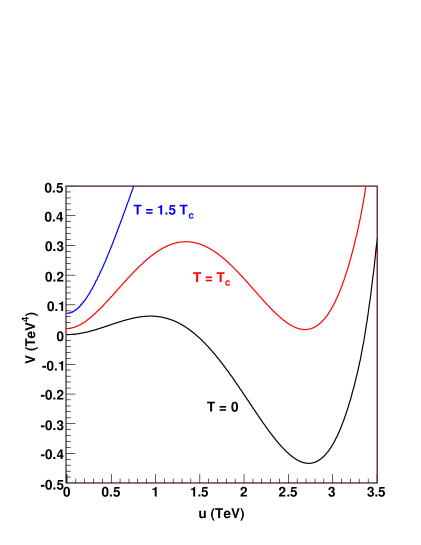
Figure 1: The effective potential as a function of the magnitude of the VEV for three different choices of temperature. The phase of the VEV at each point is chosen as the solution of the Equations of motion for that value of the magnitude.

3.2.1 Bubble Profile and Evolution

At $T_{c}$, the rate for nucleation of bubbles with $\langle\sigma\rangle\neq 0$ becomes large, and the bubbles expand to fill the universe with the true vaccuum. In this subsection we make some rough estimates of the properties of the nucleated bubbles, which are pertinent to the eventual generation of baryon asymmetry as they provide the out-of-equilibrium dynamics which results in lepton-number being unequally distributed through-out the three generations. We will simplify the treatment by considering the phase transition as a quasi-equilibrium process such that the temperature is varying slowly enough that the properties of the nucleating bubbles can be obtained by studying fixed temperature solutions at $T\simeq T_{c}$.

Assuming that the nucleated bubbles have spherical symmetry [38], the Euclidean action of the configuration becomes

$$S_{3}(T) = 4\pi\int dr\;r^{2}\Big{\{}\Big{(}\nabla\langle\sigma\rangle\Big{)}^{2}+V(\langle\sigma\rangle,T_{c})\Big{\}}$$ (32)

where $\langle\sigma\rangle$ is a function of radius $r$ that describes the configuration. The transitions will be predominantly mediated by the solutions which minimize this action, give by the solutions of the equations,

$$\frac{d^{2}u}{dr^{2}}+\frac{2}{r}\frac{du}{dr} = \frac{\delta V}{\delta u}$$

$$u^{2}\left[\frac{d^{2}\theta}{dr^{2}}+\frac{2}{r}\frac{d\theta}{dr}\right] = \frac{\delta V}{\delta\theta}$$ (33)

subject to the boundary conditions,

$$\left.\frac{du}{dr}\right|_{r=0} = 0;\qquad\left.u\right|_{r\rightarrow\infty}=0$$

$$\left.\frac{d\theta}{dr}\right|_{r=0} = 0;\qquad\left.\theta\right|_{r\rightarrow\infty}=\theta_{u=0}\>.$$ (34)

These coupled differential equations are somewhat difficult to solve. Instead of looking for detailed solutions, we will use an ansatz for the profile, and a variational approach to determine the parameters that describe it. We write the solutions in the form of two “kinks” with the proper asymmptotic behavior,

$$u(r) = \frac{u_{c}}{2}\left[1-{\rm Tanh}\left(\alpha\left(r-R\right)\right)\right]$$

$$\theta(r) = \theta_{u=0}+\frac{\theta_{c}-\theta_{u=0}}{2}\left[1-{\rm Tanh}\left(\alpha\left(r-R\right)\right)\right]$$ (35)

where the radius of the bubble is $\sim R$ and the width of the bubble wall is $\sim 1/\alpha$. In addition to imposing the form of the solution, we also assume that the bubble width is the same for $u$ and for $\theta$ (which we expect to be approximately true). We determine $\alpha$ numerically by plugging the solutions of Eq. (35) into the action Eq. (32) and finding the value of $\alpha$ which minimizes the action. For our standard parameter choice we find $\alpha\sim T/2$ and $L_{w}\equiv 1/\alpha\sim 2/T$. The profiles are plotted in Fig 2. We expect that for large bubbles, the details will become independent of $R$, which in fact proves to be true.

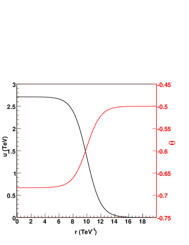
Figure 2: The bubble profile at the critical temperature $T_{c}$ for $R=10~{}{\rm TeV}^{-1}$.

Under our quasi-equilibrium assumption, the expansion of the bubble is driven by the fact that the gauge bosons acquire masses inside the bubble, and thus the free energy is minimized for large bubbles [47, 39]. By analogy with the SM EW phase transition, we estimate the bubble wall velocity $v_{w}\sim 0.05$, though we find that our final results are very insensitive to the precise value of $v_{w}$.

3.3 Diffusion Equations in the Topflavor Model

We now compute the prediction for the $L_{3}$ generated during the transition in which the Topflavor model breaks down to the SM. The underlying picture is similar to the standard EWBG picture in the SM (or MSSM). The bubble of true vacuum is expanding, and generates chiral charge through the $CP$-violating interaction of the plasma with the bubble wall. In the specific case of Topflavor, the particles which interact strongly with the wall are the Higgses, through the interactions in Eq (3.1). These charges diffuse freely in the unbroken phase and are converted into $B$ and $L_{3}$ by a combination of the Yukawa interactions and the unsuppressed sphalerons. As they pass into the broken phase, they are frozen.

In the limit $g_{1}\gg g_{2}$, we neglect the $SU(2)_{2}$ sphalerons associated with the first two families. The quark Yukawa interactions and the QCD instantons, together with the fact that all of the quarks diffuse at approximately the same rate, allows us to constrain the light quark densities in terms of the right-handed bottom density $b$,

$$Q_{1L}=Q_{2L}=-2U_{R}=-2D_{R}=-2S_{R}=-2C_{R}=-2b\,.$$ (36)

Thus, the species whose densities we will track are the left-handed top and bottom doublet, $Q\equiv t_{L}+b_{L}$, the right-handed top $t\equiv t_{R}$, the right-handed bottom $b\equiv b_{R}$, the left-handed lepton doublet $L_{3}\equiv\tau_{L}+\nu_{\tau}$, and the Higgs $h\equiv(h^{+}_{u}+h^{0}_{u}-h^{-}_{d}-h^{0}_{d})$. We assume that the $H$-$H^{\prime}$-$\Sigma$ interactions Eq. (3.1) are fast enough such that the spectator Higgses $H^{\prime}$ are kept in equilibrium with the Higgs, and thus $\Sigma=0$, $h^{\prime}\equiv({h^{\prime}}_{u}^{+}+{h^{\prime}}_{u}^{0}-{h^{\prime}}_{d}^{-}-{h^{\prime}}_{d}^{0})=h$, and we do not include the densities $\Sigma$ and $h^{\prime}$ in the diffusion equations. For relativistic particles near equilibrium, we can write the number densities in terms of a chemical potential $\mu_{i}$ as $n_{i}=k_{i}\mu_{i}T^{2}/6$ where $k_{i}$ counts the number of degrees of freedom,

$$k_{Q}=6;~{}~{}~{}k_{L}=2;~{}~{}~{}k_{t}=k_{b}=3;~{}~{}~{}k_{h}=8\,.$$ (37)

The diffusion equations will contain the interactions which are fast compared to the time scales at which the elements of the plasma are diffusing, $\tau_{i}=D_{i}/v_{w}$, where $v_{w}\sim 0.05$ is the speed of the bubble wall’s expansion and $D_{i}$ is a diffusion coefficient which characterizes the interactions with the background plasma. Typically, one expects $D_{Q}=D_{t}=D_{b}\simeq 6/T$ and $D_{L}\simeq D_{h}\simeq 110/T$ [49]. Thus, we consider the processes characterized by rate $\Gamma\gtrsim\tau_{Q}$. These interactions include the $SU(2)_{1}$ sphalerons with rate $\Gamma_{1}$, the QCD instantons with rate $\Gamma_{QCD}$, and the top quark Yukawa coupling to the Higgs with rate $\Gamma_{y}$. We continue to assume that the sphalerons associated with $SU(2)_{2}$ can be neglected. These rates are estimated to be equal to [37, 50],

$$\Gamma_{y} \simeq \frac{27}{2}\lambda_{t}^{2}\alpha_{S}\left(\frac{\zeta(3)}{\pi^{2}}\right)^{2}T=7.4~{}{\rm GeV}\,,$$ (38)

$$\Gamma_{QCD} \simeq 16\kappa^{\prime}\alpha_{S}^{4}T=0.3~{}{\rm GeV}\,,$$ (39)

$$\Gamma_{1} \simeq 30{\alpha_{1}}^{5}T=0.1~{}{\rm GeV}\,,$$ (40)

where $\lambda_{t}\sim 1$ is the top Yukawa coupling, $\alpha_{S}(T_{c})\sim 0.08$ is the strong coupling constant, and $\kappa^{\prime}\sim 1$ is a dimensionless coefficient. We have evaluated the rates for $s^{2}=0.4$ and $T_{c}=840$ GeV, as is appropriate for our example parameter set.

We approximate the bubble as large, and thus treat the problem one-dimensionally, with the $z$-axis perpendicular to the wall, whose location is at $z=0$, with the $z>0$ side in the broken phase. The rates of change of the various densities are described by the coupled set of equations

$$v_{w}Q^{\prime}-D_{Q}Q^{\prime\prime} = -\Gamma_{y}\left[\frac{Q}{k_{Q}}-\frac{h}{k_{h}}-\frac{t}{k_{t}}\right]-6\Gamma_{QCD}\left[2\frac{Q}{k_{Q}}-\frac{t}{k_{t}}-9\frac{b}{k_{b}}\right]$$

$$-6\Gamma_{1}\left[3\frac{Q}{k_{Q}}+\frac{L_{3}}{k_{L}}\right]\,,$$

$$v_{w}t^{\prime}-D_{Q}t^{\prime\prime} = -\Gamma_{y}\left[-\frac{Q}{k_{Q}}+\frac{h}{k_{h}}+\frac{t}{k_{t}}\right]+3\Gamma_{QCD}\left[2\frac{Q}{k_{Q}}-\frac{t}{k_{t}}-9\frac{b}{k_{b}}\right]\,,$$

$$v_{w}h^{\prime}-D_{h}h^{\prime\prime} = -\Gamma_{y}\left[-\frac{Q}{k_{Q}}+\frac{h}{k_{h}}+\frac{t}{k_{t}}\right]+\gamma_{h}\,,$$

$$v_{w}b^{\prime}-D_{Q}b^{\prime\prime} = 3\Gamma_{QCD}\left[2\frac{Q}{k_{Q}}-\frac{t}{k_{t}}-9\frac{b}{k_{b}}\right]\,,$$

$$v_{w}L_{3}^{\prime}-D_{L}L_{3}^{\prime\prime} = -2\Gamma_{1}\left[3\frac{Q}{k_{Q}}+\frac{L_{3}}{k_{L}}\right]\,,$$ (41)

where primes denote derivatives with respect to $z$ and $\gamma_{h}$ is the $CP$-violating source for the Higgs induced by the bubble wall, approximated as a step function,

$$\gamma_{h}=\left\{\begin{array}[]{lr}\displaystyle\tilde{\gamma}_{h_{u}}-\tilde{\gamma}_{h_{d}}{}{}{}{}{}{}{}&(-L_{w}<z\leq 0)\\ \displaystyle 0&(z>0~{}~{}\textrm{or}~{}~{}z<-L_{w})\end{array}\right.\>,$$ (42)

whose magnitude we estimate below.

3.4 $CP$-violating Sources from Spontaneous $CP$ violation

We consider the $CP$-violation arising from the spontaneous $CP$-violation associated with the phase of the VEV $\langle\sigma\rangle$. This field couples directly to the EWSB Higgses $H_{u}$ and $H_{d}$ and thus influences their number densities as they scatter off of the bubble wall. As we saw in section 3.2, the phase of $\langle\sigma\rangle$ varies as one moves from inside the bubble of true vacuum to the unbroken phase (see i.e. Figure 2),

$$\Delta\theta \equiv \theta_{c}-\theta_{u=0}=-\frac{1}{4}{\rm acos}\left[\frac{-2D^{*}+\widetilde{\lambda}^{*}u_{c}^{2}}{-2D+\widetilde{\lambda}u_{c}^{2}}\right]+\frac{1}{2}$$ (43)

and thus is space-time dependent as the bubble expands.

In computing the value of the $CP$-violating source $\gamma_{h}$, we follow the treatment first introduced by Riotto [51, 52] based on the closed time path (CTP) formalism, which allows us to capture the main non-equilibrium quantum effects. The CTP formalism distinguishes fields with arguments on the positive and negative branches of the closed time path. This doubling of fields leads to six different real-time propagators; for a generic scalar field $\phi$,

$$G_{\phi}^{>}(x,y) = -i\langle\phi(x)\phi^{{\dagger}}(y)\rangle,$$

$$G_{\phi}^{<}(x,y) = -i\langle\phi^{{\dagger}}(x)\phi(y)\rangle,$$

$$G_{\phi}^{t}(x,y) = \theta(x,y)G_{\phi}^{>}(x,y)+\theta(y,x)G_{\phi}^{<}(x,y),$$

$$G_{\phi}^{\bar{t}}(x,y) = \theta(x,y)G_{\phi}^{<}(x,y)+\theta(y,x)G_{\phi}^{>}(x,y),$$ (44)

which are conveniently written as a matrix ${G(x,y)}$:

$$\widetilde{G}(x,y)=\left(\begin{array}[]{cc}G^{t}(x,y)&-G^{<}(x,y)\\ G^{>}(x,y)&-G^{\bar{t}}(x,y)\end{array}\right).$$ (45)

From the Schwinger-Dyson equations of the path-ordered two-point functions, one obtains

$$\partial_{\mu}j^{\mu}_{\phi} = -\int d^{3}z\int^{X_{0}}_{-\infty}dz_{0}\left[\Sigma^{>}_{\phi}(X,z)G^{<}_{\phi}(z,X)-G^{>}_{\phi}(X,z)\Sigma^{<}_{\phi}(z,X)\right.$$ (46)

$$\left.+G^{<}_{\phi}(X,z)\Sigma^{>}_{\phi}(z,X)-\Sigma^{<}_{\phi}(X,z)\Sigma^{>}_{\phi}(z,X)\right].$$

Figure 3: Feynman diagrams for the leading contributions to the self-energies of $H_{u}$ in the background of a spacetime varying $\langle\Sigma\rangle$.

The leading contribution to the self energies $\tilde{\Sigma}_{H_{u}}(x,y)$ and $\tilde{\Sigma}_{H_{d}}(x,y)$ from the interactions of Eq. (3.1) are (see Figure 3)

$$\tilde{\Sigma}_{H_{u}}(x,y) = g(x,y)\tilde{G}_{H^{\prime}_{u}}(x,y)+h(x,y)\tilde{G}_{H^{\prime}_{d}}(x,y),$$

$$\tilde{\Sigma}_{H_{d}}(x,y) = \tilde{g}(x,y)\tilde{G}_{H^{\prime}_{d}}(x,y)+\tilde{h}(x,y)\tilde{G}_{H^{\prime}_{u}}(x,y),$$ (47)

where

$$g(x,y) = m^{2}_{uu^{\prime}}(x){m^{2}}^{*}_{uu^{\prime}}(y)=\left[c_{2}^{*}\mu\Sigma^{{\dagger}}(x)+c_{1}{\mu^{\prime}}^{*}\Sigma(x)\right]\left[c_{2}\mu^{*}\Sigma(y)+c_{1}^{*}{\mu^{\prime}}\Sigma^{{\dagger}}(y)\right]$$

$$h(x,y) = m^{2}_{ud^{\prime}}(x){m^{2}}^{*}_{ud^{\prime}}(y)=\left[A_{1}\Sigma(x)+A^{\prime}_{1}\Sigma^{{\dagger}}(x)\right]\left[A_{1}^{*}\Sigma^{{\dagger}}(y)+{A^{\prime}}_{1}^{*}\Sigma(y)\right]$$

$$\tilde{g}(x,y) = m^{2}_{dd^{\prime}}(x){m^{2}}^{*}_{dd^{\prime}}(y)=\left[c_{2}{\mu^{\prime}}^{*}\Sigma(x)+c_{1}^{*}{\mu}\Sigma^{{\dagger}}(x)\right]\left[c_{2}^{*}{\mu^{\prime}}\Sigma^{{\dagger}}(y)+c_{1}{\mu}^{*}\Sigma(y)\right]$$

$$\tilde{h}(x,y) = m^{2}_{du^{\prime}}(x){m^{2}}^{*}_{du^{\prime}}(y)=\left[A_{2}\Sigma(x)+A^{\prime}_{2}\Sigma^{{\dagger}}(x)\right]\left[A_{2}^{*}\Sigma^{{\dagger}}(y)+{A^{\prime}}_{2}^{*}\Sigma(y)\right]$$ (48)

The $CP$-violating part of Eq. (46), evaluated for $H_{u}$, is the imaginary part of Green functions,

$$\gamma_{h_{u}} = -i\int d^{3}z\int^{X_{0}}_{-\infty}dz_{0}\Big{\{}\left[g(x,z)-g(z,x)\right]\rm{Im}\left[G_{H^{\prime}_{u}}^{>}(x,z)G_{H_{u}}^{<}(z,x)-G_{H^{\prime}_{u}}^{<}(x,z)G_{H_{u}}^{>}(z,x)\right]$$ (49)

$$+\left[h(x,z)-h(z,x)\right]\rm{Im}\left[G_{H^{\prime}_{d}}^{>}(x,z)G_{H_{u}}^{<}(z,x)-G_{H^{\prime}_{d}}^{<}(x,z)G_{H_{u}}^{>}(z,x)\right]\Big{\}}.$$

We can express the scalar Green’s function in terms of the Bose-Einstein distribution and the spectral density of a scalar field

$$G^{\gtrless}(x,y) = \int\frac{d^{4}k}{(2\pi)^{4}}e^{-ik\cdot(x-y)}g_{B}^{\gtrless}(k_{0},\mu_{i})\rho(k_{0},\vec{k}),$$ (50)

where the equilibrium distribution functions are:

$$g_{B}^{>}(\omega,\mu) = 1+n_{B}(\omega,\mu_{i})$$ (51)

$$g_{B}^{<}(\omega,\mu) = n_{B}(\omega,\mu_{i}),$$ (52)

with $n_{B}(x)=1/[\exp(x/T)-1]$. The spectral density in the limit of small decay width is [52],

$$\rho(k_{0},\vec{k}) = i\Big{[}\frac{1}{(k^{0}+i\varepsilon+i\Gamma)^{2}-\omega^{2}(|\vec{k}|)}-\frac{1}{(k^{0}-i\varepsilon-i\Gamma)^{2}-\omega^{2}(|\vec{k}|)}\Big{]},$$ (53)

where $\omega^{2}(|\vec{k}|)=\vec{k}^{2}+M^{2}$. The mass $M$ and width $\Gamma$ are the thermal mass and width, respectively.

The coefficients $[g(x,z)-g(z,x)]$ and $[h(x,z)-h(z,x)]$ can be calculated to the first order in the expansion about $x=z$.

$$g(x,z)-g(z,x) = 2i\left[|c_{1}\mu^{\prime}|^{2}-|c_{2}\mu|^{2}\right]\sin\left[\theta(x)-\theta(z)\right]u(x)u(z)$$ (54)

$$\simeq 2i\left[|c_{1}\mu^{\prime}|^{2}-|c_{2}\mu|^{2}\right](x-z)^{\mu}\left[\partial_{\mu}\theta(x)\right]u^{2}(x)+\cdots.$$

When these are inserted in Eq. (49), the fact that the spectral density is isotropic in space, implies that only the time component is non-vanishing, and we can make the replacements,

$$g(x,z)-g(z,x) = 2i\left[|c_{1}\mu|^{2}-|c_{2}\mu|^{2}\right](x-z)^{0}]\left(\frac{\Delta\theta}{L_{w}}v_{w}\right)u^{2}(x),$$ (55)

$$h(x,z)-h(z,x) = 2i\left[|A_{1}|^{2}-|A^{\prime}_{1}|^{2}\right](x-z)^{0}\left(\frac{\Delta\theta}{L_{w}}v_{w}\right)u^{2}(x),$$ (56)

and thus,

$$\widetilde{\gamma}_{h_{u}} = \left(\frac{\Delta\theta}{L_{w}}v_{w}\right)u^{2}(x)\left\{\left[|c_{1}\mu^{\prime}|^{2}-|c_{2}\mu|^{2}\right]\mathcal{I}_{H_{u}H_{u}^{{}^{\prime}}}+\left[|A_{1}|^{2}-|A^{\prime}_{1}|^{2}\right]\mathcal{I}_{H_{u}H_{d}^{{}^{\prime}}}\right\},$$ (57)

where

$$\mathcal{I}_{H_{u}H^{\prime}_{i}} = \int_{0}^{\infty}dk\frac{k^{2}}{2\pi^{2}\omega_{H^{\prime}_{i}}\omega_{H_{u}}}\times\Big{\{}(1+2\rm{Re}[n_{B}(\omega_{H^{\prime}_{i}}+i\Gamma_{H^{\prime}_{i}})])I(\omega_{H_{u}},\Gamma_{H_{u}},\omega_{H^{\prime}_{i}},\Gamma_{H^{\prime}_{i}})$$ (58)

$$+(1+2\rm{Re}[n_{B}(\omega_{H_{u}}+i\Gamma_{H_{u}})])I(\omega_{H^{\prime}_{i}},\Gamma_{H^{\prime}_{i}},\omega_{H_{u}},\Gamma_{H_{u}})$$

$$-2(\rm{Im}[n_{B}(\omega_{H_{u}}+i\Gamma_{H_{u}})]+\rm{Im}[n_{B}(\omega_{H^{\prime}_{i}}+i\Gamma_{H^{\prime}_{i}})])G(\omega_{H_{u}},\Gamma_{H_{u}},\omega_{H^{\prime}_{i}},\Gamma_{H^{\prime}_{i}})\Big{\}}\,,$$

and the functions $I$ and $G$ are given by

$$I(a,b,c,d)=\frac{1}{2}\frac{1}{[(a+c)^{2}+(b+d)^{2}]}\sin\Big{[}2\arctan\frac{a+c}{b+d}\Big{]}$$

$$+\frac{1}{2}\frac{1}{[(a-c)^{2}+(b+d)^{2}]}\sin\Big{[}2\arctan\frac{a-c}{b+d}\Big{]}$$

$$G(a,b,c,d)=-\frac{1}{2}\frac{1}{[(a+c)^{2}+(b+d)^{2}]}\cos\Big{[}2\arctan\frac{a+c}{b+d}\Big{]}$$

$$-\frac{1}{2}\frac{1}{[(a-c)^{2}+(b+d)^{2}]}\cos\Big{[}2\arctan\frac{a-c}{b+d}\Big{]}\,.$$

In exactly the same way, we derive,

$$\widetilde{\gamma}_{h_{d}} = \left(\frac{\Delta\theta}{L_{w}}v_{w}\right)u^{2}(x)\left\{\left[|c_{1}\mu|^{2}-|c_{2}\mu^{\prime}|^{2}\right]\mathcal{I}_{H_{d}H_{d}^{{}^{\prime}}}+\left[|A_{2}|^{2}-|A^{\prime}_{2}|^{2}\right]\mathcal{I}_{H_{d}H_{u}^{{}^{\prime}}}\right\}.$$ (61)

The over-all magnitude of the $CP$-violating source depends sensitively on several parameters which have up until now not played a large role in deriving our ressults. Thus, we content ourselves with the order of magnitude estimate based on the sample parameters for the $\sigma$ potential and bubble wall velocity and profile, and assuming the thermal masses and widths are roughly TeV, and that the $\Sigma$-$H$-$H^{\prime}$ dimensionful interactions are of order TeV. Evaluating the integrals numerically, we find $\gamma_{h}\sim 0.01~{}{\rm TeV}~{}\Delta\theta/L_{w}v_{w}u_{c}^{2}$, which for the choice of sample parameters described above leads to $\gamma_{h}\sim 10^{9}$ GeV⁴, and acquires non-vanishing values only at the position of the bubble wall, where the Higgs fields are varying.

The results presented above rely on a method similar to the one used in Ref. [19] in the Minimal Supersymmetric Standard Model case. Further improvements to this method were performed in Refs. [21], by considering the all-order resummation of the Higgs mass insertion efffects. The result was a mild suppression of the results in the case of degenerate masses, as well as new relevant terms away from the degenerate mass regime. Furthermore, in Ref. [22], based on self-consistency arguments, a more detailed analysis of the relation between the CP-violating sources and the currents induced by the Higgs fields was performed, leading to the presence of higher order derivatives in the sources, as first suggested in Ref. [17]. The final result of these investigations is a suppression of the baryon asymmetry by a factor of a few in the degenerate mass regime compared to the one obtained in Ref. [19], as well as a power-law suppression with the masses when they move away from the degenerate region.

One of the weaknesses of the above described work is the lack of a rigorous derivation of the sources for the diffusion equation. A derivation of the semiclassical forces in the transport equations by means of the dynamics of the two-point function in the Schwinger-Keldysh formalism was performed in Refs. [23, 24, 25, 26]. In particular, in Ref. [26] a consistent treatment of the fermion mixing effects was performed, and a careful derivation of the sources in the diffusion equations was obtained. The final result was smaller by a factor of a few to an order of magnitude than the result obtained in Ref. [22] in the degenerate mass regime, and a stronger than power-law suppression away from the degenerate case. In our work we are interested in an order of magnitude estimate of the result for the baryon asymmetry, and for that purpose the results of this section are sufficient. However, while an enhancement of the sources by a factor of a few would be easy to obtain by a careful choice of the parameters of our model, an enhancement by several order of magnitudes woulde prove very difficult. For these reasons, it would be interesting to pursue a more general treatment using the techniques of Ref. [26] to make a detailed exploration of the full parameter space consistent with the observed baryon asymmetry.

3.5 Results

We assemble the results and make a prediction for the density of lepton number stored in the third family, $L_{3}$. We have solved the diffusion equations in two ways; the first is a brute force numerical solution of the coupled differential equations, while the second proceeds by making some simplifying approximations which allow us to determine an analytic solution to the diffusion equations. Our analytic solution simplifies the problem by assuming that $\Gamma_{y}$, $\Gamma_{QCD}$ and (for $z<0$) $\Gamma_{1}$ are all strong enough that they enforce near-equilibrium relations among the number densities of the species participating in the interactions. Thus, we have,

$$\frac{Q}{k_{Q}}-\frac{h}{k_{h}}-\frac{t}{k_{t}}\sim\frac{1}{\Gamma_{y}}\sim 0\>,$$

$$2\frac{Q}{k_{Q}}-\frac{t}{k_{t}}-9\frac{b}{k_{b}}\sim\frac{1}{\Gamma_{QCD}}\sim 0\>,$$ (62)

and for $z<0$,

$$3\frac{Q}{k_{Q}}+\frac{L_{3}}{k_{L}}\sim\frac{1}{\Gamma_{1}}\sim 0.$$ (63)

Following the treatment of the usual EW case [37], we take linear combinations of the diffusion equations (41) which are independent of $\Gamma_{y}$, $\Gamma_{QCD}$, and $\Gamma_{1}$ and use the equilibrium relations to express the remaining two equations in terms of $Q$ and $h$. The result can be expressed as a matrix differential equation,

$$M\left[\begin{array}[]{l}Q^{\prime\prime}\\ h^{\prime\prime}\end{array}\right]+N\left[\begin{array}[]{l}Q^{\prime}\\ h^{\prime}\end{array}\right]=\left[\begin{array}[]{l}-\gamma_{h}\\ 0\end{array}\right]$$ (70)

where we simplfy $\gamma_{h}$ as constant for $-L_{w}<z<0$ and $M$ and $N$ are constant matrices, functions of the $D$’s, $k$’s, and $v_{w}$,

$$M = \left[\begin{array}[]{cc}D_{Q}\left(\frac{k_{b}-9k_{t}}{9k_{b}}\right)&D_{h}+D_{Q}\left(\frac{9k_{t}+k_{b}}{9k_{h}}\right)\\ -D_{Q}\left(\frac{9k_{Q}+9k_{t}+k_{b}}{9k_{Q}}\right)-D_{L}\left(\frac{9k_{L}}{k_{Q}}\right)&D_{Q}\left(\frac{9k_{t}-k_{b}}{9k_{h}}\right)\end{array}\right]=\frac{1}{T}\left[\begin{array}[]{cc}-\frac{8}{3}&\frac{225}{2}\\ -\frac{28}{3}&2\end{array}\right]\>,$$ (75)

$$N = v_{w}\left[\begin{array}[]{cc}\frac{9k_{t}-k_{b}}{9k_{Q}}&-\frac{9k_{h}+9k_{t}+k_{b}}{9k_{h}}\\ \frac{9k_{Q}+81k_{L}+9k_{t}+k_{b}}{9k_{Q}}&\frac{k_{b}-9k_{t}}{9k_{h}}\end{array}\right]=v_{w}\left[\begin{array}[]{cc}\frac{4}{9}&-\frac{17}{12}\\ \frac{41}{9}&-\frac{1}{3}\end{array}\right]\>.$$ (80)

We convert Eq. (70) into a first order differential equation by defining $\Psi\equiv\left[Q\>,\>h\right]^{T}$, $H\equiv\Psi^{\prime}$. We solve the equations seperately for $z<L_{w}$ (region I), $-L_{w}<z<0$ (region II), and $z>0$ (region III) and match $\Psi$ and $H$ across the boundaries.

In regions I and III, $\gamma_{h}=0$, and the solutions are those of the corresponding homogeneous equation,

$$H_{\rm I,III}\left(z\right)=H_{H}\left(z\right){\cal D}_{\rm I,III} = Exp\left[-M^{-1}Nz\right]{\cal D}_{\rm I,III}$$ (81)

$$\Psi_{\rm I,III}\left(z\right) = \int_{-\infty}^{z}dx\;H_{H}\left(x\right){\cal D}_{\rm I,III}+{\cal C}_{\rm I,III}$$ (82)

where ${\cal C}_{\rm I,III}$ and ${\cal D}_{\rm I,III}$ are vectors specifying the boundary conditions. The exponential terms grow with $z$, and thus the requirement that $\Psi(z\rightarrow-\infty)\rightarrow 0$ requires ${\cal C}_{\rm I}=0$ and the requirement that $\Psi$ remain finite as $z\rightarrow+\infty$ requires ${\cal D}_{\rm III}=0$.

In region II, the solutions will be the sum of a homogeneous solution with integration constants ${\cal C}_{\rm II}$ and ${\cal D}_{\rm II}$, and a particular solution,

$$H_{P}(z) = -H_{H}(z)\int_{-L_{w}}^{z}\;dx\>H_{H}^{-1}(x)\>M^{-1}\>\left[\begin{array}[]{l}\gamma_{h}\\ 0\end{array}\right]\>.$$ (85)

So,

$$H_{\rm II}\left(z\right) = H_{H}\left(z\right){\cal D}_{\rm II}+H_{P}\left(z\right)\;,$$ (86)

$$\Psi_{\rm II}\left(z\right) = \int_{-L_{w}}^{z}dx\;\left\{H_{H}\left(x\right){\cal D}_{\rm II}+H_{P}\left(x\right)\right\}+{\cal C}_{\rm II}\;,$$ (87)

and matching this to the solutions in regions I and II determines ${\cal D}_{\rm I}={\cal D}_{\rm II}$, and,

$${\cal D}_{\rm II} = \int_{-L_{w}}^{0}dxH_{H}^{-1}\left(x\right)M^{-1}\left[\begin{array}[]{c}\gamma_{h}\\ 0\end{array}\right]\>,$$ (90)

$${\cal C}_{\rm II} = \int_{-\infty}^{-L_{w}}dxH_{H}\left(x\right){\cal D}_{\rm II}\;,$$ (91)

$${\cal C}_{\rm III} = \int_{-\infty}^{0}dxH_{H}\left(x\right){\cal D}_{\rm II}-\int_{-L_{w}}^{0}dx\int_{-L_{w}}^{x}dyH_{H}\left(x\right)H_{H}^{-1}\left(y\right)M^{-1}\left[\begin{array}[]{c}\gamma_{h}\\ 0\end{array}\right]\;.$$ (94)

Note that $\Psi(z)={\cal C}_{\rm III}$ for $z>0$, so this last expression is in fact the final densities produced by the phase transition.

Since $L_{w}$ is small, we can derive an approximate form based on the limit $L_{w}\rightarrow 0$. To leading order in $L_{w}$, we have

$${\cal C}_{\rm III}={\cal C}_{\rm II} = \int_{-\infty}^{0}dxH_{H}\left(x\right){\cal D}_{\rm II}=-L_{w}N^{-1}\left[\begin{array}[]{c}\gamma_{h}\\ 0\end{array}\right]\;,$$ (97)

where

$${\cal D}_{\rm II} = L_{w}M^{-1}\left[\begin{array}[]{c}\gamma_{h}\\ 0\end{array}\right]\>.$$ (100)

Using the expression for $N^{-1}$, we find the final lepton number density

$$L_{3}=-Q=-\frac{12L_{w}\gamma_{h}}{227v_{w}}~{}.$$ (101)

Recalling equation (3.4) that $\gamma_{h}\propto v_{w}/L_{w}$, we find that our final result is approximately independent of the diffusion constants, the bubble wall velocity, and the bubble wall width, as long as $\Gamma_{1}$ is fast enough.

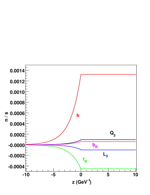
Figure 4: Particle number densities normalized to entropy as a function of spatial position $z$ for a bubble whose wall is at $z\sim 0$ and parameters as described in the text. From top to bottom, the curves represent the following densities: $h$, $Q_{3}$, $b_{R}$, $L_{3}$, and $t_{R}$.

Assembling the results, in Figure 4 we plot the densities normalized to the entropy, $s\sim 2\pi^{2}/45g_{*}T^{3}$, where $g_{*}\sim 100$. The densities $L_{3}$, $t$, and $b$ are determined using the relations Eqs. (62-63). The wall region is too small ($2\times 10^{-3}$ GeV^-1), and is only in the figure For the chosen parameters, the ratio of the lepton density to the entropy density at is given by

$$L_{3}/s\sim 10^{-4},$$ (102)

which results, after the inclusion of the dilution factor, Eq. (12) in a final baryon asymmetry after the electroweak phase transition of approximately

$$\frac{n_{B}}{s}\simeq 10^{-10},$$ (103)

exactly as observed. Of course, the particular value is highly dependent on our choice of parameters, but the ability of the Topflavor model to produce this value is not; the fact that the order of magnitude comes out correctly is indicitive of the fact that for natural values of parameters, this model can produce an appropriate baryon number.

From our numerical integration of the differential equations, we can relax our equilibrium assumptions and examine the effect of finite values for the rates, particularly $\Gamma_{1}$. In Figure  5 we present the final lepton density as a function of $\Gamma_{1}$ (artificially assuming that the $CP$-violating source, bubble parameters, and critical temperature are unchanged). For small $\Gamma_{1}$, we see that the final lepton asymmetry is linearly proportional to $\Gamma_{1}$. In this regime, the generated Higgs/top number densities are a constant background source, only a small fraction of which is converted into leptons by $\Gamma_{1}$. For large $\Gamma_{1}$ instead, the equilibrium condition is reached and the dependence on $\Gamma_{1}$ saturates. We see from Figure 5 that our chosen parameters are just at the turn-on of this saturation region.

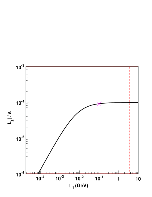
Figure 5: Lepton number density normalized to entropy as a function of $\Gamma_{1}$. The red dashed line is the bound on $\Gamma_{1}$ from non-observation of proton decay mediated by instantons, whereas the blue dotted line is the bound inferred by requiring that the broken phase minimum remain the true vacuum at $T=0$. The star indicates the sample parameter point considered in the text.

4 Discussion

We have explored the possibility that the baryon asymmetry of the Universe might have come from new gauge dynamics at the TeV scale. The primary impediment to realizing this idea is the washout by ordinary EW sphalerons, which we have avoided by having new physics which coupled asymmetrically to the three (lepton) generations. In particular, we showed that the Topflavor model, with $SU(2)_{1}\times SU(2)_{2}$ breaking at the TeV scale, can easily produce an appropriate baryon asymmetry for natural values of its parameters.

It is interesting to compare the results obtained in Eq. (102) with the much smaller ones that are obtained by similar methods in the MSSM [19]. The difference stems from three main different factors: First, the magnitude of $\Gamma_{1}$ is much larger than the EW sphaleron rate $\Gamma_{\rm ws}\simeq 10^{-4}$ GeV. As shown in Fig. 5, this induces an enhancement of a few orders of magnitude in the final result. Second, the value of $\Delta\theta\simeq 0.2$ is two orders of magnitude larger than the typical values of $\Delta\beta\simeq{\cal{O}}\left(10^{-3}\right)$ obtained in the MSSM for moderate values of the CP-odd Higgs mass. Third, in the MSSM there is a suppression proceeding from the effective cancellation of chiral charges discussed in Refs. [54, 37] that is not present in the model analyzed in this article.

We expect that the LHC can extensively test this idea. First, by discovering the SM Higgs boson and searching for the existence of other elements strongly coupled to it, the LHC can help construct the picture of the ordinary EW phase transition as first or second order. This would, for example, confirm or rule out the MSSM scenario of EW baryogenesis. Second, by discovering new elements, in the case of Topflavor, the heavy $W^{\prime}$ and $Z^{\prime}$ bosons with masses of about 2 TeV and preferred decays into third family fermions, should be easily discovered at the LHC [55]. Finally, by determining the properties of the new elements, one may determine whether or not they are viable as a mechanism of baryogenesis. In the case of Topflavor, the need for a first order phase transition in the breakdown of $SU(2)_{1}\times SU(2)_{2}$ is connected to both a small quartic for the Higgs $\sigma$ and a reasonably strong gauge coupling $g_{1}$. The first of these has the dramatic consequence that the mass of $\sigma$ is well below the symmetry-breaking scale, $m_{\sigma}^{2}\sim\lambda u^{2}$. For the parameters we explore in detail, $m_{\sigma}\sim 600$ GeV, making $\sigma$ the lightest of the new particles. It couples strongly to the Higgs sector, and to the new gauge bosons.

An extended gauge sector at the TeV scale has motivations from many mysteries in particle physics. In addition, it allows a much less constrained structure to explore the idea of baryogenesis through gauge symmetry breaking. The SM picture arising from the EW breakdown is economical, but is under assault from the null LEP Higgs searches, favoring a second order phase transition, and from the lack of sufficient $CP$ violation to produce enough asymmetry. Alternatives based on the ordinary EW transition such as in the MSSM can be viable, but remain constrained by the Higgs mass, and from the fact that the new sources of $CP$ violation remain tightly connected to low energy $CP$-violating observables. Extended gauge symmetries can naturally have first order transitions, and $CP$ violation is further removed from low energy observables. The primary obstacle is the fact that the EW sphalerons will try to erase any generated baryon asymmetry with $B-L=0$, but this is overcome if the SM matter does not couple universally to the new dynamics. Ultimately, the LHC will help in resolving this question.

5 ACKNOWLEDGMENTS

We would like to thank Junhai Kang, and David Morrisey for helpful conversations and Ignacy Sawicki for computing assistance. Work at ANL is supported in part by the US DOE, Div. of HEP, Contract W-31-109-ENG-38. J.S. would like to acknowledge Prospects in Theoretical Physics 05 for part of the initial work was done there, T.T. and C.W. would like to thank the Aspen Center for Physics were an important part of this work has been performed.

References

- [1] A. D. Sakharov, Pis’ma Zh. Eksp. Teor. Fiz. 5, 32 (1967).
- [2] M. Yoshimura, Phys. Rev. Lett. 41, 281 (1978) [Erratum-ibid. 42, 746 (1979)].
- [3] S. Dimopoulos and L. Susskind, Phys. Rev. D 18, 4500 (1978).
- [4] S. Weinberg, Phys. Rev. Lett. 42, 850 (1979).
- [5] E. W. Kolb and M. S. Turner, The Early Universe, Addison-Wesley Publishing Company (1990).
- [6] M. Fukugita and T. Yanagida, Phys. Lett. B 174, 45 (1986).
- [7] W. Buchmuller and M. Plumacher, Int. J. Mod. Phys. A 15, 5047 (2000), and references therein.
- [8] I. Affleck and M. Dine, Nucl. Phys. B 249, 361 (1985).
- [9] V. A. Kuzmin, V. A. Rubakov and M. E. Shaposhnikov, Phys. Lett. B 155, 36 (1985).
- [10] For reviews, see, M. Trodden, Rev. Mod. Phys. 71, 1463 (1999); V.A. Rubakov, M. E. Shaposhnikov, Usp. Fiz.Nauk 166 493 (1996); Phys. Usp. 39 461 (1996); A. G. Cohen, D. B. Kaplan, A. E. Nelson, Ann. Rev. Nucl. Part. Sci. 43 27 (1993).
- [11] R. Barate et al. [LEP Working Group for Higgs boson searches], Phys. Lett. B 565, 61 (2003).
- [12] M. Pietroni, Nucl. Phys. B 402, 27 (1993).
- [13] A. T. Davies, C. D. Froggatt and R. G. Moorhouse, Phys. Lett. B 372, 88 (1996).
- [14] S. J. Huber and M. G. Schmidt, Nucl. Phys. B 606, 183 (2001).
- [15] J. Kang, P. Langacker, T. j. Li and T. Liu, Phys. Rev. Lett. 94, 061801 (2005).
- [16] A. Menon, D. E. Morrissey and C. E. M. Wagner, Phys. Rev. D 70, 035005 (2004).
- [17] J. M. Cline, M. Joyce and K. Kainulainen, JHEP 0007, 018 (2000).
- [18] J. M. Cline and K. Kainulainen, Phys. Rev. Lett. 85, 5519 (2000).
- [19] M. Carena, M. Quiros, A. Riotto, I. Vilja and C. E. M. Wagner, Nucl. Phys. B 503, 387 (1997).
- [20] M. Carena, M. Quiros and C. E. M. Wagner, Nucl. Phys. B 524, 3 (1998).
- [21] M. Carena, J. M. Moreno, M. Quiros, M. Seco and C. E. M. Wagner, Nucl. Phys. B 599, 158 (2001).
- [22] M. Carena, M. Quiros, M. Seco and C. E. M. Wagner, Nucl. Phys. B 650, 24 (2003).
- [23] K. Kainulainen, T. Prokopec, M. G. Schmidt and S. Weinstock, JHEP 0106, 031 (2001).
- [24] K. Kainulainen, T. Prokopec, M. G. Schmidt and S. Weinstock, Phys. Rev. D 66, 043502 (2002).
- [25] T. Prokopec, M. G. Schmidt and S. Weinstock, Annals Phys. 314, 208 (2004) [arXiv:hep-ph/0312110]; T. Prokopec, M. G. Schmidt and S. Weinstock, Annals Phys. 314, 267 (2004) [arXiv:hep-ph/0406140].
- [26] T. Konstandin, T. Prokopec, M. G. Schmidt and M. Seco, Nucl. Phys. B 738, 1 (2006) [arXiv:hep-ph/0505103].
- [27] M. Joyce, Phys. Rev. D 55, 1875 (1997). T. Prokopec, Phys. Lett. B 483, 1 (2000).
- [28] M. Joyce and T. Prokopec, Phys. Rev. D 57, 6022 (1998).
- [29] S. Davidson, M. Losada and A. Riotto, Phys. Rev. Lett. 84, 4284 (2000).
- [30] G. Servant, JHEP 0201, 044 (2002).
- [31] M. Carena, A. Megevand, M. Quiros and C. E. M. Wagner, Nucl. Phys. B 716, 319 (2005).
- [32] A. Provenza, M. Quiros and P. Ullio, JHEP 0510, 048 (2005).
- [33] V. A. Kuzmin, V. A. Rubakov and M. E. Shaposhnikov, Phys. Lett. B 191, 171 (1987).
- [34] H. K. Dreiner and G. G. Ross, Nucl. Phys. B 410, 188 (1993).
- [35] R. S. Chivukula, E. H. Simmons and J. Terning, Phys. Rev. D 53, 5258 (1996); E. Malkawi, T. Tait and C. P. Yuan, Phys. Lett. B 385, 304 (1996); D. J. Muller and S. Nandi, Phys. Lett. B 383, 345 (1996); P. Batra, A. Delgado, D. E. Kaplan and T. M. P. Tait, JHEP 0402, 043 (2004).
- [36] D. E. Morrissey, T. M. P. Tait and C. E. M. Wagner, Phys. Rev. D 72, 095003 (2005).
- [37] P. Huet and A. E. Nelson, Phys. Rev. D 53, 4578 (1996).
- [38] S. Coleman, V. Glaser and A. Martin, Commun. Math. Phys. 58 211 (1978).
- [39] G. D. Moore and T. Prokopec, Phys. Rev. D 52, 7182 (1995) [arXiv:hep-ph/9506475]; G. D. Moore and T. Prokopec, Phys. Rev. Lett. 75, 777 (1995) [arXiv:hep-ph/9503296].
- [40] A. Kosowsky, M. S. Turner and R. Watkins, Phys. Rev. Lett. 69, 2026 (1992).
- [41] R. Apreda, M. Maggiore, A. Nicolis and A. Riotto, Nucl. Phys. B 631, 342 (2002).
- [42] A. Nicolis, Class. Quant. Grav. 21, L27 (2004).
- [43] C. Grojean and G. Servant, [arXiv:hep-ph/0607107].
- [44] L. Randall and G. Servant, [arXiv:hep-ph/0607158].
- [45] J. Shu, T. M. P. Tait and C. E. M. Wagner, in progress.
- [46] A. D. Linde, Nucl. Phys. B 216, 421 (1983) [Erratum-ibid. B 223, 544 (1983)].
- [47] M. Dine, R. G. Leigh, P. Y. Huet, A. D. Linde and D. A. Linde, Phys. Rev. D 46, 550 (1992).
- [48] A. G. Cohen, D. B. Kaplan and A. E. Nelson, Phys. Lett. B 336, 41 (1994).
- [49] M. Joyce, T. Prokopec and N. Turok, Phys. Rev. D 53, 2930 (1996).
- [50] P. Arnold, D. Son and L. G. Yaffe, Phys. Rev. D 55, 6264 (1997); D. Bodeker, G. D. Moore and K. Rummukainen, Nucl. Phys. Proc. Suppl. 83, 583 (2000); G. D. Moore, [arXiv:hep-ph/0009161].
- [51] A. Riotto, Phys. Rev. D 53, 5834 (1996).
- [52] A. Riotto, Nucl. Phys. B 518, 339 (1998).
- [53] H. Georgi, E. Jenkins and E. H. Simmons, Nucl. Phys. B 331, 541 (1990).
- [54] G. F. Giudice and M. E. Shaposhnikov, Phys. Lett. B 326, 118 (1994).
- [55] Z. Sullivan, [arXiv:hep-ph/0306266].