Probe R-parity Violating Supersymmetry Effects in Bβ†’K(βˆ—)​ℓ+β€‹β„“βˆ’β†’π΅superscript𝐾superscriptβ„“superscriptβ„“B\to K^{(*)}\ell^{+}\ell^{-} and Bsβ†’β„“+β€‹β„“βˆ’β†’subscript𝐡𝑠superscriptβ„“superscriptβ„“B_{s}\to\ell^{+}\ell^{-} Decays

Yuan-Guo Xu1, Ru-Min Wang1,2 and Ya-Dong Yang1
1 Department of Physics, Henan Normal University, XinXiang, Henan 453007, P.R.China
2 Institute of Particle Physics, Huazhong Normal University, Wuhan, Hubei 430070, P.R.China
Corresponding author. E-mail address: yangyd@henannu.edu.cn
Abstract

We study the decays Bβ†’K(βˆ—)​ℓ+β€‹β„“βˆ’β†’π΅superscript𝐾superscriptβ„“superscriptβ„“B\to K^{(*)}\ell^{+}\ell^{-} and Bsβ†’β„“+β€‹β„“βˆ’β€‹(β„“=e,ΞΌ)β†’subscript𝐡𝑠superscriptβ„“superscriptβ„“β„“π‘’πœ‡B_{s}\to\ell^{+}\ell^{-}~{}(\ell=e,\mu) in the minimal supersymmetric standard model with R-parity violation (RPV). From the recent measurements of their branching ratios, we have derived new upper bounds on the relevant RPV coupling products, which are stronger than the existing ones. Using the constrained parameter space, we predict the RPV effects on the forward-backward asymmetries π’œF​B​(Bβ†’K(βˆ—)​ℓ+β€‹β„“βˆ’)subscriptπ’œπΉπ΅β†’π΅superscript𝐾superscriptβ„“superscriptβ„“{\mathcal{A}}_{FB}(B\to K^{(*)}\ell^{+}\ell^{-}) and the branching ratios ℬ​(Bsβ†’β„“+β€‹β„“βˆ’)ℬ→subscript𝐡𝑠superscriptβ„“superscriptβ„“{\mathcal{B}}(B_{s}\to\ell^{+}\ell^{-}). Our results of the forward-backward asymmetries agree with the recent experiment data. It is also found that ℬ​(Bsβ†’β„“+β€‹β„“βˆ’)ℬ→subscript𝐡𝑠superscriptβ„“superscriptβ„“\mathcal{B}(B_{s}\to\ell^{+}\ell^{-}) could be enhanced several orders by the RPV sneutrino exchange. The RPV effects on the dilepton invariant mass spectra of Bβ†’K(βˆ—)​ℓ+β€‹β„“βˆ’β†’π΅superscript𝐾superscriptβ„“superscriptβ„“B\to K^{(*)}\ell^{+}\ell^{-} and the normalized π’œF​B​(Bβ†’K(βˆ—)​ℓ+β€‹β„“βˆ’)subscriptπ’œπΉπ΅β†’π΅superscript𝐾superscriptβ„“superscriptβ„“{\mathcal{A}}_{FB}(B\to K^{(*)}\ell^{+}\ell^{-}) are studied in detail. Our results could be used to probe RPV effects and will correlate with searches for direct RPV signals at LHC.

PACS Numbers 13.20.He 12.60.Jv 11.30.Er 12.15.Mm

1 Introduction

Flavor changing neutral current (FCNC) bβ†’s→𝑏𝑠b\to s processes are forbidden at the tree level in the standard model (SM), which proceed at a low rate via penguin or box diagrams. If additional diagrams with non-SM particles contribute, their rates as well as other properties will be modified. This feature make FCNC processes powerful means to probe new physics indirectly. The recent experimental measurements of Bβ†’K(βˆ—)​ℓ+β€‹β„“βˆ’β†’π΅superscript𝐾superscriptβ„“superscriptβ„“B\to K^{(*)}\ell^{+}\ell^{-} decays[1, 2, 3, 4] agree with the SM predictions within their error bars, therefore, these measurements will afford an opportunity to constrain new physics scenarios beyond the SM.

Semileptonic rare decays Bβ†’K(βˆ—)​ℓ+β€‹β„“βˆ’β†’π΅superscript𝐾superscriptβ„“superscriptβ„“B\to K^{(*)}\ell^{+}\ell^{-} have been extensively studied previously. The dominant perturbative SM contribution had been evaluated years ago[5], and later QCD corrections have been provided [6, 7, 8]. π’ͺ​(1/mb2)π’ͺ1subscriptsuperscriptπ‘š2𝑏\mathcal{O}(1/m^{2}_{b}) corrections have been first calculated in Ref.[9] and then in Refs.[10, 11]. Long distance contributions can have different origins according to the value of the dilepton invariant mass. The contributions of charmonium resonances to these decays by means of Vector Meson Dominance (VMD) have been studied carefully[10, 12, 13, 14]. Far from the resonance region, instead, c​c¯𝑐¯𝑐c\bar{c} long-distance effects are investigated using a heavy quark expansion in inverse powers of the charm-quark mass (π’ͺ​(1/mc2)π’ͺ1subscriptsuperscriptπ‘š2𝑐\mathcal{O}(1/m^{2}_{c}) corrections) [15]. Analyses of new physics contribution have been performed in different models, for example, the two-Higgs doublet model[16] , the supersymmetric (SUSY) models [17, 18], the SUSY SO(10) grand unification theory [19] and the top quark two-Higgs doublet model [20].

The effects of RPV SUSY in B𝐡B meson decays have been extensively investigated in the literature [21, 22]. The decays Bβ†’K(βˆ—)​ℓ+β€‹β„“βˆ’β†’π΅superscript𝐾superscriptβ„“superscriptβ„“B\to K^{(*)}\ell^{+}\ell^{-} and Bsβ†’β„“+β€‹β„“βˆ’β†’subscript𝐡𝑠superscriptβ„“superscriptβ„“B_{s}\to\ell^{+}\ell^{-} are all induced at the parton level by bβ†’s​ℓ+β€‹β„“βˆ’β†’π‘π‘ superscriptβ„“superscriptβ„“b\to s\ell^{+}\ell^{-} process, and they involve the same set of the RPV coupling products. In this paper we will study the decays Bβ†’K(βˆ—)​ℓ+β€‹β„“βˆ’β†’π΅superscript𝐾superscriptβ„“superscriptβ„“B\to K^{(*)}\ell^{+}\ell^{-} and Bsβ†’β„“+β€‹β„“βˆ’β†’subscript𝐡𝑠superscriptβ„“superscriptβ„“B_{s}\to\ell^{+}\ell^{-} in the RPV SUSY model. Using the recent experimental data, we will obtain the new upper limits on the relevant RPV coupling products. Then we will use the constrained regions of the parameters to examine the RPV effects on the branching ratios of Bsβ†’β„“+β€‹β„“βˆ’β†’subscript𝐡𝑠superscriptβ„“superscriptβ„“B_{s}\to\ell^{+}\ell^{-} decays and the forward-backward asymmetries (π’œF​B)subscriptπ’œπΉπ΅(\mathcal{A}_{FB}) of Bβ†’K(βˆ—)​ℓ+β€‹β„“βˆ’β†’π΅superscript𝐾superscriptβ„“superscriptβ„“B\to K^{(*)}\ell^{+}\ell^{-}. In addition, we will compare the SM predictions with the RPV predictions about dilepton invariant mass spectra and the normalized forward-backward asymmetries in Bβ†’K(βˆ—)​ℓ+β€‹β„“βˆ’β†’π΅superscript𝐾superscriptβ„“superscriptβ„“B\to K^{(*)}\ell^{+}\ell^{-} decays.

The paper is arranged as follows. In Section 2, we introduce the effective Hamiltonian and calculate the expressions for Bβ†’K(βˆ—)​ℓ+β€‹β„“βˆ’β†’π΅superscript𝐾superscriptβ„“superscriptβ„“B\to K^{(*)}\ell^{+}\ell^{-} and Bsβ†’β„“+β€‹β„“βˆ’β†’subscript𝐡𝑠superscriptβ„“superscriptβ„“B_{s}\to\ell^{+}\ell^{-} processes in the RPV SUSY. In Section 3, we tabulate the theoretical inputs and deal with the numerical results. We display the constrained parameter spaces which satisfy all the available experimental data, and then we use the constrained parameter spaces to predict the RPV effects on π’œF​Bsubscriptπ’œπΉπ΅\mathcal{A}_{FB}(Bβ†’K(βˆ—)​ℓ+β€‹β„“βˆ’β†’π΅superscript𝐾superscriptβ„“superscriptβ„“B\to K^{(*)}\ell^{+}\ell^{-}) and ℬ​(Bsβ†’β„“+β€‹β„“βˆ’)ℬ→subscript𝐡𝑠superscriptβ„“superscriptβ„“\mathcal{B}(B_{s}\to\ell^{+}\ell^{-}), which have not been well measured yet. We also show the RPV effects on dilepton invariant mass spectra and the normalized forward-backward asymmetries in Bβ†’K(βˆ—)​ℓ+β€‹β„“βˆ’β†’π΅superscript𝐾superscriptβ„“superscriptβ„“B\to K^{(*)}\ell^{+}\ell^{-} decays. Section 4 contains our summary and conclusion.

2 The theoretical frame for Bβ†’K(βˆ—)​ℓ+β€‹β„“βˆ’β†’π΅superscript𝐾superscriptβ„“superscriptβ„“B\to K^{(*)}\ell^{+}\ell^{-} and Bsβ†’β„“+β€‹β„“βˆ’β†’subscript𝐡𝑠superscriptβ„“superscriptβ„“B_{s}\to\ell^{+}\ell^{-}

2.1 The decay branching ratios in the SM

2.1.1 The semileptonic decays Bβ†’K(βˆ—)​ℓ+β€‹β„“βˆ’β†’π΅superscript𝐾superscriptβ„“superscriptβ„“B\to K^{(*)}\ell^{+}\ell^{-}

In the SM, at the quark level, the rare semileptonic decays bβ†’s​ℓ+β€‹β„“βˆ’β†’π‘π‘ superscriptβ„“superscriptβ„“b\to s\ell^{+}\ell^{-} can be described by the effective Hamiltonian

β„‹e​f​fS​M​(bβ†’s​ℓ+β€‹β„“βˆ’)=βˆ’GF2​Vt​sβˆ—β€‹Vt​bβ€‹βˆ‘i=110Ci​(ΞΌ)​π’ͺi,subscriptsuperscriptℋ𝑆𝑀𝑒𝑓𝑓→𝑏𝑠superscriptβ„“superscriptβ„“subscript𝐺𝐹2subscriptsuperscript𝑉𝑑𝑠subscript𝑉𝑑𝑏subscriptsuperscript10𝑖1subscriptπΆπ‘–πœ‡subscriptπ’ͺ𝑖\displaystyle\mathcal{H}^{SM}_{eff}(b\to s\ell^{+}\ell^{-})=-\frac{G_{F}}{\sqrt{2}}V^{*}_{ts}V_{tb}\sum^{10}_{i=1}C_{i}(\mu)\mathcal{O}_{i}, (1)

where the operator base π’ͺisubscriptπ’ͺ𝑖\mathcal{O}_{i} is given in [7]. We will use the Wilson coefficients Ci​(ΞΌ)subscriptπΆπ‘–πœ‡C_{i}(\mu) calculated in the naive dimensional regularization (NDR) scheme [7], and the long-distance resonance effects on C9e​f​f​(ΞΌ)subscriptsuperscript𝐢𝑒𝑓𝑓9πœ‡C^{eff}_{9}(\mu) given in Refs.[12, 14]. The Hamiltonian leads to the following free quark decay amplitude:

β„³S​M​(bβ†’s​ℓ+β€‹β„“βˆ’)superscriptℳ𝑆𝑀→𝑏𝑠superscriptβ„“superscriptβ„“\displaystyle\mathcal{M}^{SM}(b\to s\ell^{+}\ell^{-}) =GF​αe2​πVt​sβˆ—Vt​b{C9e​f​f(sΒ―Ξ³ΞΌPLb)(β„“Β―Ξ³ΞΌβ„“)+C10(sΒ―Ξ³ΞΌPLb)(β„“Β―Ξ³ΞΌΞ³5β„“)\displaystyle=\frac{G_{F}\alpha_{e}}{\sqrt{2}\pi}V^{*}_{ts}V_{tb}\Big{\{}C^{eff}_{9}(\bar{s}\gamma_{\mu}P_{L}b)(\bar{\ell}\gamma^{\mu}\ell)+C_{10}(\bar{s}\gamma_{\mu}P_{L}b)(\bar{\ell}\gamma^{\mu}\gamma_{5}\ell) (2)
βˆ’2m^bC7e​f​f(sΒ―iσμ​νq^Ξ½s^PRb)(β„“Β―Ξ³ΞΌβ„“)},\displaystyle-2\hat{m}_{b}C^{eff}_{7}\left(\bar{s}i\sigma_{\mu\nu}\frac{\hat{q}^{\nu}}{\hat{s}}P_{R}b\right)(\bar{\ell}\gamma^{\mu}\ell)\Big{\}},

with PL,R≑(1βˆ“Ξ³5)/2,s=q2formulae-sequencesubscript𝑃𝐿𝑅minus-or-plus1subscript𝛾52𝑠superscriptπ‘ž2P_{L,R}\equiv(1\mp\gamma_{5})/2,s=q^{2} and q=p++pβˆ’π‘žsubscript𝑝subscript𝑝q=p_{+}+p_{-} (pΒ±subscript𝑝plus-or-minusp_{\pm} the four-momenta of the leptons). In our following calculations, we take ms/mb=0subscriptπ‘šπ‘ subscriptπ‘šπ‘0m_{s}/m_{b}=0, but keep the lepton masses. The hat denotes normalization in terms of the B-meson mass, mBsubscriptπ‘šπ΅m_{B}, e.g. s^=s/mB2^𝑠𝑠superscriptsubscriptπ‘šπ΅2\hat{s}=s/m_{B}^{2}, m^q=mq/mBsubscript^π‘šπ‘žsubscriptπ‘šπ‘žsubscriptπ‘šπ΅\hat{m}_{q}=m_{q}/m_{B}.

Exclusive decays Bβ†’K(βˆ—)​ℓ+β€‹β„“βˆ’β†’π΅superscript𝐾superscriptβ„“superscriptβ„“B\to K^{(*)}\ell^{+}\ell^{-} are described in terms of matrix elements of the quark operators in Eq.(2) over meson states, which can be parameterized by the form factors. It is worth noting the form factors involving the Bβ†’K(βˆ—)→𝐡superscript𝐾B\to K^{(*)} transitions have been updated recently in [23].

Using Eq.(2), one can get the amplitudes of exclusive Bβ†’K(βˆ—)​ℓ+β€‹β„“βˆ’β†’π΅superscript𝐾superscriptβ„“superscriptβ„“B\to K^{(*)}\ell^{+}\ell^{-} decays

β„³S​M​(Bβ†’K(βˆ—)​ℓ+β€‹β„“βˆ’)=GF​αe2​2​π​Vt​sβˆ—β€‹Vt​b​mB​[𝒯1​μ​(ℓ¯​γμ​ℓ)+𝒯2​μ​(ℓ¯​γμ​γ5​ℓ)],superscriptℳ𝑆𝑀→𝐡superscript𝐾superscriptβ„“superscriptβ„“subscript𝐺𝐹subscript𝛼𝑒22πœ‹subscriptsuperscript𝑉𝑑𝑠subscript𝑉𝑑𝑏subscriptπ‘šπ΅delimited-[]subscript𝒯1πœ‡Β―β„“superscriptπ›Ύπœ‡β„“subscript𝒯2πœ‡Β―β„“superscriptπ›Ύπœ‡subscript𝛾5β„“\displaystyle\mathcal{M}^{SM}(B\to K^{(*)}\ell^{+}\ell^{-})=\frac{G_{F}\alpha_{e}}{2\sqrt{2}~{}\pi}V^{*}_{ts}V_{tb}m_{B}\left[\mathcal{T}_{1\mu}(\bar{\ell}\gamma^{\mu}\ell)+\mathcal{T}_{2\mu}(\bar{\ell}\gamma^{\mu}\gamma_{5}\ell)\right], (3)

where for Bβ†’K​ℓ+β€‹β„“βˆ’β†’π΅πΎsuperscriptβ„“superscriptβ„“B\to K\ell^{+}\ell^{-},

𝒯1​μ=A′​(s^)​p^ΞΌ+B′​(s^)​q^ΞΌ,subscript𝒯1πœ‡superscript𝐴′^𝑠subscript^π‘πœ‡superscript𝐡′^𝑠subscript^π‘žπœ‡\displaystyle\mathcal{T}_{1\mu}=A^{\prime}(\hat{s})\hat{p}_{\mu}+B^{\prime}(\hat{s})\hat{q}_{\mu}, (4)
𝒯2​μ=C′​(s^)​p^ΞΌ+D′​(s^)​q^ΞΌ,subscript𝒯2πœ‡superscript𝐢′^𝑠subscript^π‘πœ‡superscript𝐷′^𝑠subscript^π‘žπœ‡\displaystyle\mathcal{T}_{2\mu}=C^{\prime}(\hat{s})\hat{p}_{\mu}+D^{\prime}(\hat{s})\hat{q}_{\mu}, (5)

and for Bβ†’Kβˆ—β€‹β„“+β€‹β„“βˆ’β†’π΅superscript𝐾superscriptβ„“superscriptβ„“B\to K^{*}\ell^{+}\ell^{-},

𝒯1​μsubscript𝒯1πœ‡\displaystyle\mathcal{T}_{1\mu} =\displaystyle= A​(s^)β€‹Ο΅ΞΌβ€‹Οβ€‹Ξ±β€‹Ξ²β€‹Ο΅βˆ—Οβ€‹p^Bα​p^Kβˆ—Ξ²βˆ’i​B​(s^)β€‹Ο΅ΞΌβˆ—+i​C​(s^)​(Ο΅βˆ—β‹…p^B)​p^ΞΌ+i​D​(s^)​(Ο΅βˆ—β‹…p^B)​q^ΞΌ,𝐴^𝑠subscriptitalic-Ο΅πœ‡πœŒπ›Όπ›½superscriptitalic-Ο΅absent𝜌subscriptsuperscript^𝑝𝛼𝐡subscriptsuperscript^𝑝𝛽superscript𝐾𝑖𝐡^𝑠subscriptsuperscriptitalic-Ο΅πœ‡π‘–πΆ^𝑠⋅superscriptitalic-Ο΅subscript^𝑝𝐡subscript^π‘πœ‡π‘–π·^𝑠⋅superscriptitalic-Ο΅subscript^𝑝𝐡subscript^π‘žπœ‡\displaystyle A(\hat{s})\epsilon_{\mu\rho\alpha\beta}\epsilon^{*\rho}\hat{p}^{\alpha}_{B}\hat{p}^{\beta}_{K^{*}}-iB(\hat{s})\epsilon^{*}_{\mu}+iC(\hat{s})(\epsilon^{*}\cdot\hat{p}_{B})\hat{p}_{\mu}+iD(\hat{s})(\epsilon^{*}\cdot\hat{p}_{B})\hat{q}_{\mu}, (6)
𝒯2​μsubscript𝒯2πœ‡\displaystyle\mathcal{T}_{2\mu} =\displaystyle= E​(s^)β€‹Ο΅ΞΌβ€‹Οβ€‹Ξ±β€‹Ξ²β€‹Ο΅βˆ—Οβ€‹p^Bα​p^Kβˆ—Ξ²βˆ’i​F​(s^)β€‹Ο΅ΞΌβˆ—+i​G​(s^)​(Ο΅βˆ—β‹…p^B)​p^ΞΌ+i​H​(s^)​(Ο΅βˆ—β‹…p^B)​q^ΞΌ,𝐸^𝑠subscriptitalic-Ο΅πœ‡πœŒπ›Όπ›½superscriptitalic-Ο΅absent𝜌subscriptsuperscript^𝑝𝛼𝐡subscriptsuperscript^𝑝𝛽superscript𝐾𝑖𝐹^𝑠subscriptsuperscriptitalic-Ο΅πœ‡π‘–πΊ^𝑠⋅superscriptitalic-Ο΅subscript^𝑝𝐡subscript^π‘πœ‡π‘–π»^𝑠⋅superscriptitalic-Ο΅subscript^𝑝𝐡subscript^π‘žπœ‡\displaystyle E(\hat{s})\epsilon_{\mu\rho\alpha\beta}\epsilon^{*\rho}\hat{p}^{\alpha}_{B}\hat{p}^{\beta}_{K^{*}}-iF(\hat{s})\epsilon^{*}_{\mu}+iG(\hat{s})(\epsilon^{*}\cdot\hat{p}_{B})\hat{p}_{\mu}+iH(\hat{s})(\epsilon^{*}\cdot\hat{p}_{B})\hat{q}_{\mu}, (7)

with p=pB+pK(βˆ—)𝑝subscript𝑝𝐡subscript𝑝superscript𝐾p=p_{B}+p_{K^{(*)}}. Note that, using the equation of motion for lepton fields, the q^ΞΌsubscript^π‘žπœ‡\hat{q}_{\mu} terms in 𝒯1​μsubscript𝒯1πœ‡\mathcal{T}_{1\mu} vanish, and those in 𝒯2​μsubscript𝒯2πœ‡\mathcal{T}_{2\mu} become suppressed by one power of the lepton mass.

The auxiliary functions in 𝒯1​μsubscript𝒯1πœ‡\mathcal{T}_{1\mu} and 𝒯2​μsubscript𝒯2πœ‡\mathcal{T}_{2\mu} are defined as [18]

A′​(s^)superscript𝐴′^𝑠\displaystyle A^{\prime}(\hat{s}) =\displaystyle= C9e​f​f​(s^)​f+​(s^)+2​m^b1+m^K​C7e​f​f​fT​(s^),subscriptsuperscript𝐢𝑒𝑓𝑓9^𝑠subscript𝑓^𝑠2subscript^π‘šπ‘1subscript^π‘šπΎsubscriptsuperscript𝐢𝑒𝑓𝑓7subscript𝑓𝑇^𝑠\displaystyle C^{eff}_{9}(\hat{s})f_{+}(\hat{s})+\frac{2\hat{m}_{b}}{1+\hat{m}_{K}}C^{eff}_{7}f_{T}(\hat{s}), (8)
B′​(s^)superscript𝐡′^𝑠\displaystyle B^{\prime}(\hat{s}) =\displaystyle= C9e​f​f​(s^)​fβˆ’β€‹(s^)βˆ’2​m^bs^​(1βˆ’m^K)​C7e​f​f​fT​(s^),subscriptsuperscript𝐢𝑒𝑓𝑓9^𝑠subscript𝑓^𝑠2subscript^π‘šπ‘^𝑠1subscript^π‘šπΎsubscriptsuperscript𝐢𝑒𝑓𝑓7subscript𝑓𝑇^𝑠\displaystyle C^{eff}_{9}(\hat{s})f_{-}(\hat{s})-\frac{2\hat{m}_{b}}{\hat{s}}(1-\hat{m}_{K})C^{eff}_{7}f_{T}(\hat{s}), (9)
C′​(s^)superscript𝐢′^𝑠\displaystyle C^{\prime}(\hat{s}) =\displaystyle= C10​f+​(s^),subscript𝐢10subscript𝑓^𝑠\displaystyle C_{10}f_{+}(\hat{s}), (10)
D′​(s^)superscript𝐷′^𝑠\displaystyle D^{\prime}(\hat{s}) =\displaystyle= C10​fβˆ’β€‹(s^),subscript𝐢10subscript𝑓^𝑠\displaystyle C_{10}f_{-}(\hat{s}), (11)
A​(s^)𝐴^𝑠\displaystyle A(\hat{s}) =\displaystyle= 21+m^Kβˆ—β€‹C9e​f​f​(s^)​V​(s^)+4​m^bs^​C7e​f​f​T1​(s^),21subscript^π‘šsuperscript𝐾subscriptsuperscript𝐢𝑒𝑓𝑓9^𝑠𝑉^𝑠4subscript^π‘šπ‘^𝑠subscriptsuperscript𝐢𝑒𝑓𝑓7subscript𝑇1^𝑠\displaystyle\frac{2}{1+\hat{m}_{K^{*}}}C^{eff}_{9}(\hat{s})V(\hat{s})+\frac{4\hat{m}_{b}}{\hat{s}}C^{eff}_{7}T_{1}(\hat{s}), (12)
B​(s^)𝐡^𝑠\displaystyle B(\hat{s}) =\displaystyle= (1+m^Kβˆ—)​[C9e​f​f​(s^)​A1​(s^)+2​m^bs^​(1βˆ’m^Kβˆ—)​C7e​f​f​T2​(s^)],1subscript^π‘šsuperscript𝐾delimited-[]subscriptsuperscript𝐢𝑒𝑓𝑓9^𝑠subscript𝐴1^𝑠2subscript^π‘šπ‘^𝑠1subscript^π‘šsuperscript𝐾subscriptsuperscript𝐢𝑒𝑓𝑓7subscript𝑇2^𝑠\displaystyle(1+\hat{m}_{K^{*}})\left[C^{eff}_{9}(\hat{s})A_{1}(\hat{s})+\frac{2\hat{m}_{b}}{\hat{s}}(1-\hat{m}_{K^{*}})C^{eff}_{7}T_{2}(\hat{s})\right], (13)
C​(s^)𝐢^𝑠\displaystyle C(\hat{s}) =\displaystyle= 11βˆ’m^Kβˆ—2​[(1βˆ’m^Kβˆ—)​C9e​f​f​(s^)​A2​(s^)+2​m^b​C7e​f​f​(T3​(s^)+1βˆ’m^Kβˆ—s^​T2​(s^))],11subscriptsuperscript^π‘š2superscript𝐾delimited-[]1subscript^π‘šsuperscript𝐾subscriptsuperscript𝐢𝑒𝑓𝑓9^𝑠subscript𝐴2^𝑠2subscript^π‘šπ‘subscriptsuperscript𝐢𝑒𝑓𝑓7subscript𝑇3^𝑠1subscript^π‘šsuperscript𝐾^𝑠subscript𝑇2^𝑠\displaystyle\frac{1}{1-\hat{m}^{2}_{K^{*}}}\left[(1-\hat{m}_{K^{*}})C^{eff}_{9}(\hat{s})A_{2}(\hat{s})+2\hat{m}_{b}C^{eff}_{7}\left(T_{3}(\hat{s})+\frac{1-\hat{m}_{K^{*}}}{\hat{s}}T_{2}(\hat{s})\right)\right], (14)
D​(s^)𝐷^𝑠\displaystyle D(\hat{s}) =\displaystyle= 1s^[C9e​f​f(s^)((1+m^Kβˆ—)A1(s^)βˆ’(1βˆ’m^Kβˆ—)A2(s^)βˆ’2m^Kβˆ—A0(s^))\displaystyle\frac{1}{\hat{s}}\Big{[}C^{eff}_{9}(\hat{s})\Big{(}(1+\hat{m}_{K^{*}})A_{1}(\hat{s})-(1-\hat{m}_{K^{*}})A_{2}(\hat{s})-2\hat{m}_{K^{*}}A_{0}(\hat{s})\Big{)} (15)
βˆ’2m^bC7e​f​fT3(s^)],\displaystyle-2\hat{m}_{b}C^{eff}_{7}T_{3}(\hat{s})\Big{]},
E​(s^)𝐸^𝑠\displaystyle E(\hat{s}) =\displaystyle= 21+m^Kβˆ—β€‹C10​V​(s^),21subscript^π‘šsuperscript𝐾subscript𝐢10𝑉^𝑠\displaystyle\frac{2}{1+\hat{m}_{K^{*}}}C_{10}V(\hat{s}), (16)
F​(s^)𝐹^𝑠\displaystyle F(\hat{s}) =\displaystyle= (1+m^Kβˆ—)​C10​A1​(s^),1subscript^π‘šsuperscript𝐾subscript𝐢10subscript𝐴1^𝑠\displaystyle(1+\hat{m}_{K^{*}})C_{10}A_{1}(\hat{s}), (17)
G​(s^)𝐺^𝑠\displaystyle G(\hat{s}) =\displaystyle= 11+m^Kβˆ—β€‹C10​A2​(s^),11subscript^π‘šsuperscript𝐾subscript𝐢10subscript𝐴2^𝑠\displaystyle\frac{1}{1+\hat{m}_{K^{*}}}C_{10}A_{2}(\hat{s}), (18)
H​(s^)𝐻^𝑠\displaystyle H(\hat{s}) =\displaystyle= 1s^​C10​[(1+m^Kβˆ—)​A1​(s^)βˆ’(1βˆ’m^Kβˆ—)​A2​(s^)βˆ’2​m^Kβˆ—β€‹A0​(s^)].1^𝑠subscript𝐢10delimited-[]1subscript^π‘šsuperscript𝐾subscript𝐴1^𝑠1subscript^π‘šsuperscript𝐾subscript𝐴2^𝑠2subscript^π‘šsuperscript𝐾subscript𝐴0^𝑠\displaystyle\frac{1}{\hat{s}}C_{10}\Big{[}(1+\hat{m}_{K^{*}})A_{1}(\hat{s})-(1-\hat{m}_{K^{*}})A_{2}(\hat{s})-2\hat{m}_{K^{*}}A_{0}(\hat{s})\Big{]}. (19)

It’s noted that the inclusion of the full s-quark mass dependence in the above formulae can be done by substituting mbβ†’mb+msβ†’subscriptπ‘šπ‘subscriptπ‘šπ‘subscriptπ‘šπ‘ m_{b}\to m_{b}+m_{s} into all terms proportional to C7e​f​f​T1superscriptsubscript𝐢7𝑒𝑓𝑓subscript𝑇1C_{7}^{eff}T_{1} and C7e​f​f​fTsubscriptsuperscript𝐢𝑒𝑓𝑓7subscript𝑓𝑇C^{eff}_{7}f_{T} and mbβ†’mbβˆ’msβ†’subscriptπ‘šπ‘subscriptπ‘šπ‘subscriptπ‘šπ‘ m_{b}\to m_{b}-m_{s} in C7e​f​f​T2,3superscriptsubscript𝐢7𝑒𝑓𝑓subscript𝑇23C_{7}^{eff}T_{2,3}, since π’ͺ7∼s¯​σμ​ν​[(mb+ms)+(mbβˆ’ms)​γ5]​qν​bsimilar-tosubscriptπ’ͺ7¯𝑠subscriptπœŽπœ‡πœˆdelimited-[]subscriptπ‘šπ‘subscriptπ‘šπ‘ subscriptπ‘šπ‘subscriptπ‘šπ‘ subscript𝛾5superscriptπ‘žπœˆπ‘\mathcal{O}_{7}\sim\overline{s}\sigma_{\mu\nu}[(m_{b}+m_{s})+(m_{b}-m_{s})\gamma_{5}]q^{\nu}b.

The kinematic variables (s^,u^)^𝑠^𝑒(\hat{s},\hat{u}) are chosen to be

s^^𝑠\displaystyle\hat{s} =\displaystyle= q^2=(p^++p^βˆ’)2,superscript^π‘ž2superscriptsubscript^𝑝subscript^𝑝2\displaystyle\hat{q}^{2}=(\hat{p}_{+}+\hat{p}_{-})^{2}, (20)
u^^𝑒\displaystyle\hat{u} =\displaystyle= (p^Bβˆ’p^βˆ’)2βˆ’(p^Bβˆ’p^+)2,superscriptsubscript^𝑝𝐡subscript^𝑝2superscriptsubscript^𝑝𝐡subscript^𝑝2\displaystyle(\hat{p}_{B}-\hat{p}_{-})^{2}-(\hat{p}_{B}-\hat{p}_{+})^{2}, (21)

which are bounded as

(2​m^β„“)2≀superscript2subscript^π‘šβ„“2absent\displaystyle(2\hat{m}_{\ell})^{2}\leq s^^𝑠\displaystyle\hat{s} ≀(1βˆ’m^K(βˆ—))2,absentsuperscript1subscript^π‘šsuperscript𝐾2\displaystyle\leq(1-\hat{m}_{K^{(*)}})^{2}, (22)
βˆ’u^​(s^)≀^𝑒^𝑠absent\displaystyle-\hat{u}(\hat{s})\leq u^^𝑒\displaystyle\hat{u} ≀u^​(s^),absent^𝑒^𝑠\displaystyle\leq\hat{u}(\hat{s}), (23)

with m^β„“=mβ„“/mBsubscript^π‘šβ„“subscriptπ‘šβ„“subscriptπ‘šπ΅\hat{m}_{\ell}=m_{\ell}/m_{B} and

u^​(s^)^𝑒^𝑠\displaystyle\hat{u}(\hat{s}) =\displaystyle= λ​(1βˆ’4​m^β„“2s^),πœ†14subscriptsuperscript^π‘š2β„“^𝑠\displaystyle\sqrt{\lambda\big{(}1-4\frac{\hat{m}^{2}_{\ell}}{\hat{s}}\big{)}}, (24)
Ξ»πœ†\displaystyle\lambda ≑\displaystyle\equiv λ​(1,m^K(βˆ—)2,s^)πœ†1subscriptsuperscript^π‘š2superscript𝐾^𝑠\displaystyle\lambda(1,\hat{m}^{2}_{K^{(*)}},\hat{s}) (25)
=\displaystyle= 1+m^K(βˆ—)4+s^2βˆ’2​s^βˆ’2​m^K(βˆ—)2​(1+s^).1subscriptsuperscript^π‘š4superscript𝐾superscript^𝑠22^𝑠2subscriptsuperscript^π‘š2superscript𝐾1^𝑠\displaystyle 1+\hat{m}^{4}_{K^{(*)}}+\hat{s}^{2}-2\hat{s}-2\hat{m}^{2}_{K^{(*)}}(1+\hat{s}).

The variable u^^𝑒\hat{u} corresponds to ΞΈπœƒ\theta, the angle between the momentum of the B-meson and the lepton β„“+superscriptβ„“\ell^{+} in the dilepton center-of-mass system (CMS) frame, through the relation u^=βˆ’u^​(s)​cos​θ^𝑒^𝑒𝑠cosπœƒ\hat{u}=-\hat{u}(s)\mbox{cos}\theta [14]. Keeping the lepton mass, we find the double differential decay branching ratios ℬKsuperscriptℬ𝐾\mathcal{B}^{K} and ℬKβˆ—superscriptℬsuperscript𝐾\mathcal{B}^{K^{*}} for the decays Bβ†’K​ℓ+β€‹β„“βˆ’β†’π΅πΎsuperscriptβ„“superscriptβ„“B\to K\ell^{+}\ell^{-} and Bβ†’Kβˆ—β€‹β„“+β€‹β„“βˆ’β†’π΅superscript𝐾superscriptβ„“superscriptβ„“B\to K^{*}\ell^{+}\ell^{-}, respectively, as

d2​ℬS​MKd​s^​d​u^superscript𝑑2subscriptsuperscriptℬ𝐾𝑆𝑀𝑑^𝑠𝑑^𝑒\displaystyle\frac{d^{2}\mathcal{B}^{K}_{SM}}{d\hat{s}d\hat{u}} =\displaystyle= Ο„B​GF2​αe2​mB5211​π5​|Vt​sβˆ—β€‹Vt​b|2subscript𝜏𝐡subscriptsuperscript𝐺2𝐹superscriptsubscript𝛼𝑒2superscriptsubscriptπ‘šπ΅5superscript211superscriptπœ‹5superscriptsubscriptsuperscript𝑉𝑑𝑠subscript𝑉𝑑𝑏2\displaystyle\tau_{B}\frac{G^{2}_{F}\alpha_{e}^{2}m_{B}^{5}}{2^{11}\pi^{5}}|V^{*}_{ts}V_{tb}|^{2} (26)
Γ—{(|Aβ€²|2+|Cβ€²|2)(Ξ»βˆ’u^2)\displaystyle\times\Bigg{\{}(|A^{\prime}|^{2}+|C^{\prime}|^{2})(\lambda-\hat{u}^{2})
+|Cβ€²|24m^β„“2(2+2m^K2βˆ’s^)+Re(Cβ€²Dβ€²β£βˆ—)8m^β„“2(1βˆ’m^K2)+|Dβ€²|24m^β„“2s^},\displaystyle+|C^{\prime}|^{2}4\hat{m}^{2}_{\ell}(2+2\hat{m}^{2}_{K}-\hat{s})+Re(C^{\prime}D^{\prime*})8\hat{m}^{2}_{\ell}(1-\hat{m}^{2}_{K})+|D^{\prime}|^{2}4\hat{m}^{2}_{\ell}\hat{s}\Bigg{\}},
d2​ℬS​MKβˆ—d​s^​d​u^superscript𝑑2subscriptsuperscriptℬsuperscript𝐾𝑆𝑀𝑑^𝑠𝑑^𝑒\displaystyle\frac{d^{2}\mathcal{B}^{K^{*}}_{SM}}{d\hat{s}d\hat{u}} =\displaystyle= Ο„B​GF2​αe2​mB5211​π5​|Vt​sβˆ—β€‹Vt​b|2subscript𝜏𝐡subscriptsuperscript𝐺2𝐹superscriptsubscript𝛼𝑒2superscriptsubscriptπ‘šπ΅5superscript211superscriptπœ‹5superscriptsubscriptsuperscript𝑉𝑑𝑠subscript𝑉𝑑𝑏2\displaystyle\tau_{B}\frac{G^{2}_{F}\alpha_{e}^{2}m_{B}^{5}}{2^{11}\pi^{5}}|V^{*}_{ts}V_{tb}|^{2} (27)
Γ—{|A|24(s^(Ξ»+u^2)+4m^β„“2Ξ»)+|E|24(s^(Ξ»+u^2)βˆ’4m^β„“2Ξ»)\displaystyle\times\left\{\frac{|A|^{2}}{4}\Big{(}\hat{s}(\lambda+\hat{u}^{2})+4\hat{m}^{2}_{\ell}\lambda\Big{)}+\frac{|E|^{2}}{4}\Big{(}\hat{s}(\lambda+\hat{u}^{2})-4\hat{m}^{2}_{\ell}\lambda\Big{)}\right.
+14​m^Kβˆ—2​[|B|2​(Ξ»βˆ’u^2+8​m^Kβˆ—2​(s^+2​m^β„“2))+|F|2​(Ξ»βˆ’u^2+8​m^Kβˆ—2​(s^βˆ’4​m^β„“2))]14subscriptsuperscript^π‘š2superscript𝐾delimited-[]superscript𝐡2πœ†superscript^𝑒28subscriptsuperscript^π‘š2superscript𝐾^𝑠2subscriptsuperscript^π‘š2β„“superscript𝐹2πœ†superscript^𝑒28subscriptsuperscript^π‘š2superscript𝐾^𝑠4subscriptsuperscript^π‘š2β„“\displaystyle+\frac{1}{4\hat{m}^{2}_{K^{*}}}\Big{[}|B|^{2}\Big{(}\lambda-\hat{u}^{2}+8\hat{m}^{2}_{K^{*}}(\hat{s}+2\hat{m}^{2}_{\ell})\Big{)}+|F|^{2}\Big{(}\lambda-\hat{u}^{2}+8\hat{m}^{2}_{K^{*}}(\hat{s}-4\hat{m}^{2}_{\ell})\Big{)}\Big{]}
βˆ’2​s^​u^​[R​e​(B​Eβˆ—)+R​e​(A​Fβˆ—)]2^𝑠^𝑒delimited-[]𝑅𝑒𝐡superscript𝐸𝑅𝑒𝐴superscript𝐹\displaystyle-2\hat{s}\hat{u}\Big{[}Re(BE^{*})+Re(AF^{*})\Big{]}
+Ξ»4​m^Kβˆ—2​[|C|2​(Ξ»βˆ’u^2)+|G|2​(Ξ»βˆ’u^2+4​m^β„“2​(2+2​m^Kβˆ—2βˆ’s^))]πœ†4subscriptsuperscript^π‘š2superscript𝐾delimited-[]superscript𝐢2πœ†superscript^𝑒2superscript𝐺2πœ†superscript^𝑒24subscriptsuperscript^π‘š2β„“22subscriptsuperscript^π‘š2superscript𝐾^𝑠\displaystyle+\frac{\lambda}{4\hat{m}^{2}_{K^{*}}}\Big{[}|C|^{2}(\lambda-\hat{u}^{2})+|G|^{2}(\lambda-\hat{u}^{2}+4\hat{m}^{2}_{\ell}(2+2\hat{m}^{2}_{K^{*}}-\hat{s})\Big{)}\Big{]}
βˆ’12​m^Kβˆ—2[Re(BCβˆ—)(1βˆ’m^Kβˆ—2βˆ’s^)(Ξ»βˆ’u^2)\displaystyle-\frac{1}{2\hat{m}^{2}_{K^{*}}}\Big{[}Re(BC^{*})(1-\hat{m}^{2}_{K^{*}}-\hat{s})(\lambda-\hat{u}^{2})
+Re(FGβˆ—)((1βˆ’m^Kβˆ—2βˆ’s^)(Ξ»βˆ’u^2)+4m^β„“2Ξ»)]\displaystyle~{}~{}~{}~{}~{}~{}~{}~{}~{}+Re(FG^{*})\Big{(}(1-\hat{m}^{2}_{K^{*}}-\hat{s})(\lambda-\hat{u}^{2})+4\hat{m}^{2}_{\ell}\lambda\Big{)}\Big{]}
βˆ’2m^β„“2m^Kβˆ—2Ξ»[Re(FHβˆ—)βˆ’Re(GHβˆ—)(1βˆ’m^Kβˆ—2)]+|H|2m^β„“2m^Kβˆ—2s^Ξ»}.\displaystyle\left.-2\frac{\hat{m}^{2}_{\ell}}{\hat{m}^{2}_{K^{*}}}\lambda\Big{[}Re(FH^{*})-Re(GH^{*})(1-\hat{m}^{2}_{K^{*}})\Big{]}+|H|^{2}\frac{\hat{m}^{2}_{\ell}}{\hat{m}^{2}_{K^{*}}}\hat{s}\lambda\right\}.

Our results of the double differential decay branching ratios are consistent with the ones in Ref.[18].

2.1.2 The pure leptonic decays Bsβ†’β„“+β€‹β„“βˆ’β†’subscript𝐡𝑠superscriptβ„“superscriptβ„“B_{s}\to\ell^{+}\ell^{-}

In the SM, the effective Hamiltonian have been given by [24]

β„‹e​f​fS​M​(Bsβ†’β„“+β€‹β„“βˆ’)=βˆ’GF2​αe2​π​sin2​θW​Vt​sβˆ—β€‹Vt​b​Y​(xt)​(s¯​b)Vβˆ’A​(ℓ¯​ℓ)Vβˆ’A+h.c.,formulae-sequencesubscriptsuperscriptℋ𝑆𝑀𝑒𝑓𝑓→subscript𝐡𝑠superscriptβ„“superscriptβ„“subscript𝐺𝐹2subscript𝛼𝑒2πœ‹superscriptsin2subscriptπœƒπ‘Šsubscriptsuperscript𝑉𝑑𝑠subscriptπ‘‰π‘‘π‘π‘Œsubscriptπ‘₯𝑑subscript¯𝑠𝑏𝑉𝐴subscriptΒ―β„“β„“π‘‰π΄β„Žπ‘\displaystyle\mathcal{H}^{SM}_{eff}(B_{s}\to\ell^{+}\ell^{-})=-\frac{G_{F}}{\sqrt{2}}\frac{\alpha_{e}}{2\pi\mbox{sin}^{2}\theta_{W}}V^{*}_{ts}V_{tb}Y(x_{t})(\overline{s}b)_{V-A}(\overline{\ell}\ell)_{V-A}+h.c., (28)

where xt=mt2mW2,mt≑mΒ―t​(mt)formulae-sequencesubscriptπ‘₯𝑑superscriptsubscriptπ‘šπ‘‘2superscriptsubscriptπ‘šπ‘Š2subscriptπ‘šπ‘‘subscriptΒ―π‘šπ‘‘subscriptπ‘šπ‘‘x_{t}=\frac{m_{t}^{2}}{m_{W}^{2}},m_{t}\equiv\overline{m}_{t}(m_{t}), (s¯​b)Vβˆ’A≑s¯​γμ​(1βˆ’Ξ³5)​bsubscript¯𝑠𝑏𝑉𝐴¯𝑠subscriptπ›Ύπœ‡1subscript𝛾5𝑏(\bar{s}b)_{V-A}\equiv\bar{s}\gamma_{\mu}(1-\gamma_{5})b. The pure leptonic decay amplitudes can be written as

β„³S​M​(Bsβ†’β„“+β€‹β„“βˆ’)=hS​M​(ℓ¯​​pB​(1βˆ’Ξ³5)​ℓ),superscriptℳ𝑆𝑀→subscript𝐡𝑠superscriptβ„“superscriptβ„“subscriptβ„Žπ‘†π‘€Β―β„“subscript𝑝𝐡1subscript𝛾5β„“\displaystyle\mathcal{M}^{SM}(B_{s}\to\ell^{+}\ell^{-})=h_{SM}\left(\bar{\ell}\not\!p\,_{B}(1-\gamma_{5})\ell\right), (29)

with

hS​M=βˆ’GF2​αe2​π​sin2​θW​Vt​sβˆ—β€‹Vt​b​Y​(xt)​(i​fBs).subscriptβ„Žπ‘†π‘€subscript𝐺𝐹2subscript𝛼𝑒2πœ‹superscriptsin2subscriptπœƒπ‘Šsubscriptsuperscript𝑉𝑑𝑠subscriptπ‘‰π‘‘π‘π‘Œsubscriptπ‘₯𝑑𝑖subscript𝑓subscript𝐡𝑠\displaystyle h_{SM}=-\frac{G_{F}}{\sqrt{2}}\frac{\alpha_{e}}{2\pi\mbox{sin}^{2}\theta_{W}}V^{*}_{ts}V_{tb}Y(x_{t})(if_{B_{s}}). (30)

Then we can get the branching ratios for Bsβ†’β„“+β€‹β„“βˆ’β†’subscript𝐡𝑠superscriptβ„“superscriptβ„“B_{s}\to\ell^{+}\ell^{-}

ℬS​M​(Bsβ†’β„“+β€‹β„“βˆ’)superscriptℬ𝑆𝑀→subscript𝐡𝑠superscriptβ„“superscriptβ„“\displaystyle\mathcal{B}^{SM}(B_{s}\to\ell^{+}\ell^{-}) =\displaystyle= Ο„Bs16​π​mBs​1βˆ’4​m^β„“2​|β„³S​M​(Bsβ†’β„“+β€‹β„“βˆ’)|2subscript𝜏subscript𝐡𝑠16πœ‹subscriptπ‘šsubscript𝐡𝑠14subscriptsuperscript^π‘š2β„“superscriptsuperscriptℳ𝑆𝑀→subscript𝐡𝑠superscriptβ„“superscriptβ„“2\displaystyle\frac{\tau_{B_{s}}}{16\pi m_{B_{s}}}\sqrt{1-4\hat{m}^{2}_{\ell}}\left|\mathcal{M}^{SM}(B_{s}\to\ell^{+}\ell^{-})\right|^{2} (31)
=\displaystyle= Ο„Bs​GF2π​(Ξ±e4​π​sin2​θW)2​fBs2​mβ„“2​mBs​1βˆ’4​m^β„“2​|Vt​sβˆ—β€‹Vt​b|2​Y2​(xt).subscript𝜏subscript𝐡𝑠subscriptsuperscript𝐺2πΉπœ‹superscriptsubscript𝛼𝑒4πœ‹superscriptsin2subscriptπœƒπ‘Š2subscriptsuperscript𝑓2subscript𝐡𝑠subscriptsuperscriptπ‘š2β„“subscriptπ‘šsubscript𝐡𝑠14subscriptsuperscript^π‘š2β„“superscriptsubscriptsuperscript𝑉𝑑𝑠subscript𝑉𝑑𝑏2superscriptπ‘Œ2subscriptπ‘₯𝑑\displaystyle\tau_{B_{s}}\frac{G^{2}_{F}}{\pi}\left(\frac{\alpha_{e}}{4\pi\mbox{sin}^{2}\theta_{W}}\right)^{2}f^{2}_{B_{s}}m^{2}_{\ell}m_{B_{s}}\sqrt{1-4\hat{m}^{2}_{\ell}}\left|V^{*}_{ts}V_{tb}\right|^{2}Y^{2}(x_{t}).

2.2 The decay amplitudes in RPV SUSY

In the most general superpotential of the minimal supersymmetric Standard Model (MSSM), the RPV superpotential is given by [25]

𝒲​Rpsubscript𝒲subscript𝑅𝑝\displaystyle\mathcal{W}_{\not\!R_{p}\,} =\displaystyle= ΞΌi​L^i​H^u+12​λ[i​j]​k​L^i​L^j​E^kc+Ξ»i​j​k′​L^i​Q^j​D^kc+12​λi​[j​k]′′​U^ic​D^jc​D^kc,subscriptπœ‡π‘–subscript^𝐿𝑖subscript^𝐻𝑒12subscriptπœ†delimited-[]π‘–π‘—π‘˜subscript^𝐿𝑖subscript^𝐿𝑗subscriptsuperscript^πΈπ‘π‘˜subscriptsuperscriptπœ†β€²π‘–π‘—π‘˜subscript^𝐿𝑖subscript^𝑄𝑗subscriptsuperscript^π·π‘π‘˜12subscriptsuperscriptπœ†β€²β€²π‘–delimited-[]π‘—π‘˜subscriptsuperscript^π‘ˆπ‘π‘–subscriptsuperscript^𝐷𝑐𝑗subscriptsuperscript^π·π‘π‘˜\displaystyle\mu_{i}\hat{L}_{i}\hat{H}_{u}+\frac{1}{2}\lambda_{[ij]k}\hat{L}_{i}\hat{L}_{j}\hat{E}^{c}_{k}+\lambda^{\prime}_{ijk}\hat{L}_{i}\hat{Q}_{j}\hat{D}^{c}_{k}+\frac{1}{2}\lambda^{\prime\prime}_{i[jk]}\hat{U}^{c}_{i}\hat{D}^{c}_{j}\hat{D}^{c}_{k}, (32)

where L^^𝐿\hat{L} and Q^^𝑄\hat{Q} are the SU(2) doublet lepton and quark superfields, respectively. E^csuperscript^𝐸𝑐\hat{E}^{c}, U^csuperscript^π‘ˆπ‘\hat{U}^{c} and D^csuperscript^𝐷𝑐\hat{D}^{c} are the singlet superfields, while i𝑖i, j𝑗j and kπ‘˜k are generation indices and c𝑐c denotes a charge conjugate field.

The bilinear RPV superpotential terms ΞΌi​L^i​H^usubscriptπœ‡π‘–subscript^𝐿𝑖subscript^𝐻𝑒\mu_{i}\hat{L}_{i}\hat{H}_{u} can be rotated away by suitable redefining the lepton and Higgs superfields [26]. However, the rotation will generate a soft SUSY breaking bilinear term which would affect our calculation through loop level. However, the processes discussed in this paper could be induced by tree-level RPV couplings, so that we would neglect sub-leading RPV loop contributions in this study.

The Ξ»πœ†\lambda and Ξ»β€²superscriptπœ†β€²\lambda^{\prime} couplings in Eq.(32) break the lepton number, while the Ξ»β€²β€²superscriptπœ†β€²β€²\lambda^{\prime\prime} couplings break the baryon number. There are 27 Ξ»i​j​kβ€²subscriptsuperscriptπœ†β€²π‘–π‘—π‘˜\lambda^{\prime}_{ijk} couplings, 9 Ξ»i​j​ksubscriptπœ†π‘–π‘—π‘˜\lambda_{ijk} and 9 Ξ»i​j​kβ€²β€²subscriptsuperscriptπœ†β€²β€²π‘–π‘—π‘˜\lambda^{\prime\prime}_{ijk} couplings. Ξ»[i​j]​ksubscriptπœ†delimited-[]π‘–π‘—π‘˜\lambda_{[ij]k} are antisymmetric with respect to their first two indices, and Ξ»i​[j​k]β€²β€²subscriptsuperscriptπœ†β€²β€²π‘–delimited-[]π‘—π‘˜\lambda^{\prime\prime}_{i[jk]} are antisymmetric with j𝑗j and kπ‘˜k.

Refer to caption
Figure 1: The RPV contributions to Bβ†’K(βˆ—)​ℓ+β€‹β„“βˆ’β†’π΅superscript𝐾superscriptβ„“superscriptβ„“B\to K^{(*)}\ell^{+}\ell^{-} due to sneutrino and squark exchange.
Refer to caption
Figure 2: The RPV contributions to Bsβ†’β„“+β€‹β„“βˆ’β†’subscript𝐡𝑠superscriptβ„“superscriptβ„“B_{s}\to\ell^{+}\ell^{-} due to sneutrino and squark exchange.

From Eq.(32), we can obtain the relevant four fermion effective Hamiltonian for bβ†’s​ℓ​ℓ→𝑏𝑠ℓℓb\to s\ell\ell process due to the squarks and sneutrinos exchanges

β„‹e​f​f​Rpsubscriptsuperscriptβ„‹subscript𝑅𝑝𝑒𝑓𝑓\displaystyle\mathcal{H}^{\not\!R_{p}\,}_{eff} =\displaystyle= 12β€‹βˆ‘iΞ»j​i​k′​λl​i​nβ€²β£βˆ—mu~i​L2​(dΒ―k​γμ​PR​dn)​(β„“Β―l​γμ​PL​ℓj)12subscript𝑖subscriptsuperscriptπœ†β€²π‘—π‘–π‘˜subscriptsuperscriptπœ†β€²π‘™π‘–π‘›subscriptsuperscriptπ‘š2subscript~𝑒𝑖𝐿subscriptΒ―π‘‘π‘˜superscriptπ›Ύπœ‡subscript𝑃𝑅subscript𝑑𝑛subscript¯ℓ𝑙subscriptπ›Ύπœ‡subscript𝑃𝐿subscriptℓ𝑗\displaystyle\frac{1}{2}\sum_{i}\frac{\lambda^{\prime}_{jik}\lambda^{\prime*}_{lin}}{m^{2}_{\tilde{u}_{iL}}}(\bar{d}_{k}\gamma^{\mu}P_{R}d_{n})(\bar{\ell}_{l}\gamma_{\mu}P_{L}\ell_{j}) (33)
+12β€‹βˆ‘i{Ξ»i​j​k​λi​m​nβ€²β£βˆ—mΞ½~i​L2​(dΒ―m​PR​dn)​(β„“Β―k​PL​ℓj)+Ξ»i​j​kβˆ—β€‹Ξ»i​m​nβ€²mΞ½~i​L2​(dΒ―n​PL​dm)​(β„“Β―j​PR​ℓk)}.12subscript𝑖subscriptπœ†π‘–π‘—π‘˜subscriptsuperscriptπœ†β€²π‘–π‘šπ‘›subscriptsuperscriptπ‘š2subscript~πœˆπ‘–πΏsubscriptΒ―π‘‘π‘šsubscript𝑃𝑅subscript𝑑𝑛subscriptΒ―β„“π‘˜subscript𝑃𝐿subscriptℓ𝑗subscriptsuperscriptπœ†π‘–π‘—π‘˜subscriptsuperscriptπœ†β€²π‘–π‘šπ‘›subscriptsuperscriptπ‘š2subscript~πœˆπ‘–πΏsubscript¯𝑑𝑛subscript𝑃𝐿subscriptπ‘‘π‘šsubscript¯ℓ𝑗subscript𝑃𝑅subscriptβ„“π‘˜\displaystyle+\frac{1}{2}\sum_{i}\left\{\frac{\lambda_{ijk}\lambda^{\prime*}_{imn}}{m^{2}_{\tilde{\nu}_{iL}}}(\bar{d}_{m}P_{R}d_{n})(\bar{\ell}_{k}P_{L}\ell_{j})+\frac{\lambda^{*}_{ijk}\lambda^{\prime}_{imn}}{m^{2}_{\tilde{\nu}_{iL}}}(\bar{d}_{n}P_{L}d_{m})(\bar{\ell}_{j}P_{R}\ell_{k})\right\}.

The RPV feynman diagrams for Bβ†’K(βˆ—)​ℓ+β€‹β„“βˆ’β†’π΅superscript𝐾superscriptβ„“superscriptβ„“B\to K^{(*)}\ell^{+}\ell^{-} and Bsβ†’β„“+β€‹β„“βˆ’β†’subscript𝐡𝑠superscriptβ„“superscriptβ„“B_{s}\to\ell^{+}\ell^{-} are displayed in Fig.2 and Fig.2, respectively.

From Eq.(33), we can obtain the RPV decay amplitude for Bβ†’K​ℓ+β€‹β„“βˆ’β†’π΅πΎsuperscriptβ„“superscriptβ„“B\to K\ell^{+}\ell^{-}

ℳ​Rp​(Bβ†’K​ℓ+β€‹β„“βˆ’)=Ξ”u~​(β„“Β―k​(​pB+​pK)​(1βˆ’Ξ³5)​ℓj)+Δν~​(β„“Β―k​(1βˆ’Ξ³5)​ℓj)+Δν~′​(β„“Β―k​(1+Ξ³5)​ℓj),superscriptβ„³subscript𝑅𝑝→𝐡𝐾superscriptβ„“superscriptβ„“subscriptΞ”~𝑒subscriptΒ―β„“π‘˜subscript𝑝𝐡subscript𝑝𝐾1subscript𝛾5subscriptℓ𝑗subscriptΞ”~𝜈subscriptΒ―β„“π‘˜1subscript𝛾5subscriptℓ𝑗subscriptsuperscriptΞ”β€²~𝜈subscriptΒ―β„“π‘˜1subscript𝛾5subscriptℓ𝑗\displaystyle\mathcal{M}^{\not\!R_{p}\,}(B\to K\ell^{+}\ell^{-})=\Delta_{\tilde{u}}\Big{(}\bar{\ell}_{k}(\not\!p\,_{B}+\not\!p\,_{K})(1-\gamma_{5})\ell_{j}\Big{)}+\Delta_{\tilde{\nu}}\Big{(}\bar{\ell}_{k}(1-\gamma_{5})\ell_{j}\Big{)}+\Delta^{\prime}_{\tilde{\nu}}\Big{(}\bar{\ell}_{k}(1+\gamma_{5})\ell_{j}\Big{)}, (34)

with

Ξ”u~=βˆ‘iΞ»j​i​3′​λk​i​2β€²β£βˆ—8​mu~i​L2​f+Bβ†’K​(s^),subscriptΞ”~𝑒subscript𝑖subscriptsuperscriptπœ†β€²π‘—π‘–3superscriptsubscriptπœ†π‘˜π‘–2β€²8subscriptsuperscriptπ‘š2subscript~𝑒𝑖𝐿superscriptsubscript𝑓→𝐡𝐾^𝑠\displaystyle\Delta_{\tilde{u}}=\sum_{i}\frac{\lambda^{\prime}_{ji3}\lambda_{ki2}^{\prime*}}{8m^{2}_{\tilde{u}_{iL}}}f_{+}^{B\to K}(\hat{s}), (35)
Δν~=βˆ‘iΞ»i​j​k​λi​32β€²β£βˆ—8​mΞ½~i​L2​f+Bβ†’K​(s^)​mB2βˆ’mK2mΒ―bβˆ’mΒ―s,subscriptΞ”~𝜈subscript𝑖subscriptπœ†π‘–π‘—π‘˜superscriptsubscriptπœ†π‘–32β€²8subscriptsuperscriptπ‘š2subscript~πœˆπ‘–πΏsuperscriptsubscript𝑓→𝐡𝐾^𝑠subscriptsuperscriptπ‘š2𝐡subscriptsuperscriptπ‘š2𝐾subscriptΒ―π‘šπ‘subscriptΒ―π‘šπ‘ \displaystyle\Delta_{\tilde{\nu}}=\sum_{i}\frac{\lambda_{ijk}\lambda_{i32}^{\prime*}}{8m^{2}_{\tilde{\nu}_{iL}}}f_{+}^{B\to K}(\hat{s})\frac{m^{2}_{B}-m^{2}_{K}}{\overline{m}_{b}-\overline{m}_{s}}, (36)
Δν~β€²=βˆ‘iΞ»i​k​jβˆ—β€‹Ξ»i​23β€²8​mΞ½~i​L2​f+Bβ†’K​(s^)​mB2βˆ’mK2mΒ―bβˆ’mΒ―s,subscriptsuperscriptΞ”β€²~𝜈subscript𝑖subscriptsuperscriptπœ†π‘–π‘˜π‘—subscriptsuperscriptπœ†β€²π‘–238subscriptsuperscriptπ‘š2subscript~πœˆπ‘–πΏsuperscriptsubscript𝑓→𝐡𝐾^𝑠subscriptsuperscriptπ‘š2𝐡subscriptsuperscriptπ‘š2𝐾subscriptΒ―π‘šπ‘subscriptΒ―π‘šπ‘ \displaystyle\Delta^{\prime}_{\tilde{\nu}}=\sum_{i}\frac{\lambda^{*}_{ikj}\lambda^{\prime}_{i23}}{8m^{2}_{\tilde{\nu}_{iL}}}f_{+}^{B\to K}(\hat{s})\frac{m^{2}_{B}-m^{2}_{K}}{\overline{m}_{b}-\overline{m}_{s}}, (37)

and mΒ―bsubscriptΒ―π‘šπ‘\overline{m}_{b} and mΒ―ssubscriptΒ―π‘šπ‘ \overline{m}_{s} the quark’s running masses at the scale mbsubscriptπ‘šπ‘m_{b}.

For Bβ†’Kβˆ—β€‹β„“+β€‹β„“βˆ’β†’π΅superscript𝐾superscriptβ„“superscriptβ„“B\to K^{*}\ell^{+}\ell^{-}, the RPV amplitude is

ℳ​Rp​(Bβ†’Kβˆ—β€‹β„“+β€‹β„“βˆ’)=𝒯3​μ​(β„“Β―k​γμ​(1βˆ’Ξ³5)​ℓj)+Ων~​(β„“Β―k​(1βˆ’Ξ³5)​ℓj)+Ων~′​(β„“Β―k​(1+Ξ³5)​ℓj),superscriptβ„³subscript𝑅𝑝→𝐡superscript𝐾superscriptβ„“superscriptβ„“subscript𝒯3πœ‡subscriptΒ―β„“π‘˜superscriptπ›Ύπœ‡1subscript𝛾5subscriptℓ𝑗subscriptΞ©~𝜈subscriptΒ―β„“π‘˜1subscript𝛾5subscriptℓ𝑗subscriptsuperscriptΞ©β€²~𝜈subscriptΒ―β„“π‘˜1subscript𝛾5subscriptℓ𝑗\displaystyle\mathcal{M}^{\not\!R_{p}\,}(B\to K^{*}\ell^{+}\ell^{-})=\mathcal{T}_{3\mu}\Big{(}\bar{\ell}_{k}\gamma^{\mu}(1-\gamma_{5})\ell_{j}\Big{)}+~{}\Omega_{\tilde{\nu}}\Big{(}\bar{\ell}_{k}(1-\gamma_{5})\ell_{j}\Big{)}+~{}\Omega^{\prime}_{\tilde{\nu}}\Big{(}\bar{\ell}_{k}(1+\gamma_{5})\ell_{j}\Big{)}, (38)

where

𝒯3​μsubscript𝒯3πœ‡\displaystyle\mathcal{T}_{3\mu} =\displaystyle= I​(s^)β€‹Ο΅ΞΌβ€‹Οβ€‹Ξ±β€‹Ξ²β€‹Ο΅βˆ—Οβ€‹p^Bα​p^Kβˆ—Ξ²βˆ’i​J​(s^)β€‹Ο΅ΞΌβˆ—+i​K​(s^)​(Ο΅βˆ—β‹…p^B)​p^ΞΌ+i​L​(s^)​(Ο΅βˆ—β‹…p^B)​q^ΞΌ,𝐼^𝑠subscriptitalic-Ο΅πœ‡πœŒπ›Όπ›½superscriptitalic-Ο΅absent𝜌subscriptsuperscript^𝑝𝛼𝐡subscriptsuperscript^𝑝𝛽superscript𝐾𝑖𝐽^𝑠subscriptsuperscriptitalic-Ο΅πœ‡π‘–πΎ^𝑠⋅superscriptitalic-Ο΅subscript^𝑝𝐡subscript^π‘πœ‡π‘–πΏ^𝑠⋅superscriptitalic-Ο΅subscript^𝑝𝐡subscript^π‘žπœ‡\displaystyle I(\hat{s})\epsilon_{\mu\rho\alpha\beta}\epsilon^{*\rho}\hat{p}^{\alpha}_{B}\hat{p}^{\beta}_{K^{*}}-iJ(\hat{s})\epsilon^{*}_{\mu}+iK(\hat{s})(\epsilon^{*}\cdot\hat{p}_{B})\hat{p}_{\mu}+iL(\hat{s})(\epsilon^{*}\cdot\hat{p}_{B})\hat{q}_{\mu}, (39)
Ων~subscriptΞ©~𝜈\displaystyle\Omega_{\tilde{\nu}} =\displaystyle= βˆ‘iΞ»i​j​k​λi​32β€²β£βˆ—8​mΞ½~i​L2​[βˆ’i2​A0Bβ†’Kβˆ—β€‹(s^)mΒ―b+mΒ―s​λ12​mB2],subscript𝑖subscriptπœ†π‘–π‘—π‘˜superscriptsubscriptπœ†π‘–32β€²8subscriptsuperscriptπ‘š2subscript~πœˆπ‘–πΏdelimited-[]𝑖2superscriptsubscript𝐴0→𝐡superscript𝐾^𝑠subscriptΒ―π‘šπ‘subscriptΒ―π‘šπ‘ superscriptπœ†12subscriptsuperscriptπ‘š2𝐡\displaystyle\sum_{i}\frac{\lambda_{ijk}\lambda_{i32}^{\prime*}}{8m^{2}_{\tilde{\nu}_{iL}}}\left[-\frac{i}{2}\frac{A_{0}^{B\to K^{*}}(\hat{s})}{\overline{m}_{b}+\overline{m}_{s}}\lambda^{\frac{1}{2}}m^{2}_{B}\right], (40)
Ων~β€²subscriptsuperscriptΞ©β€²~𝜈\displaystyle\Omega^{\prime}_{\tilde{\nu}} =\displaystyle= βˆ‘iΞ»i​k​jβˆ—β€‹Ξ»i​23β€²8​mΞ½~i​L2​[i2​A0Bβ†’Kβˆ—β€‹(s^)mΒ―b+mΒ―s​λ12​mB2],subscript𝑖subscriptsuperscriptπœ†π‘–π‘˜π‘—subscriptsuperscriptπœ†β€²π‘–238subscriptsuperscriptπ‘š2subscript~πœˆπ‘–πΏdelimited-[]𝑖2superscriptsubscript𝐴0→𝐡superscript𝐾^𝑠subscriptΒ―π‘šπ‘subscriptΒ―π‘šπ‘ superscriptπœ†12subscriptsuperscriptπ‘š2𝐡\displaystyle\sum_{i}\frac{\lambda^{*}_{ikj}\lambda^{\prime}_{i23}}{8m^{2}_{\tilde{\nu}_{iL}}}\left[\frac{i}{2}\frac{A_{0}^{B\to K^{*}}(\hat{s})}{\overline{m}_{b}+\overline{m}_{s}}\lambda^{\frac{1}{2}}m^{2}_{B}\right], (41)

and the auxiliary functions are given as

I​(s^)𝐼^𝑠\displaystyle I(\hat{s}) =\displaystyle= βˆ‘iΞ»j​i​3′​λk​i​2β€²β£βˆ—8​mu~i​L2​[2​VBβ†’Kβˆ—β€‹(s^)mB+mKβˆ—β€‹mB2],subscript𝑖subscriptsuperscriptπœ†β€²π‘—π‘–3superscriptsubscriptπœ†π‘˜π‘–2β€²8subscriptsuperscriptπ‘š2subscript~𝑒𝑖𝐿delimited-[]2superscript𝑉→𝐡superscript𝐾^𝑠subscriptπ‘šπ΅subscriptπ‘šsuperscript𝐾subscriptsuperscriptπ‘š2𝐡\displaystyle\sum_{i}\frac{\lambda^{\prime}_{ji3}\lambda_{ki2}^{\prime*}}{8m^{2}_{\tilde{u}_{iL}}}\left[\frac{2V^{B\to K^{*}}(\hat{s})}{m_{B}+m_{K^{*}}}m^{2}_{B}\right], (42)
J​(s^)𝐽^𝑠\displaystyle J(\hat{s}) =\displaystyle= βˆ‘iΞ»j​i​3′​λk​i​2β€²β£βˆ—8​mu~i​L2​[βˆ’(mB+mKβˆ—)​A1Bβ†’Kβˆ—β€‹(s^)],subscript𝑖subscriptsuperscriptπœ†β€²π‘—π‘–3superscriptsubscriptπœ†π‘˜π‘–2β€²8subscriptsuperscriptπ‘š2subscript~𝑒𝑖𝐿delimited-[]subscriptπ‘šπ΅subscriptπ‘šsuperscript𝐾superscriptsubscript𝐴1→𝐡superscript𝐾^𝑠\displaystyle\sum_{i}\frac{\lambda^{\prime}_{ji3}\lambda_{ki2}^{\prime*}}{8m^{2}_{\tilde{u}_{iL}}}\left[-(m_{B}+m_{K^{*}})A_{1}^{B\to K^{*}}(\hat{s})\right], (43)
K​(s^)𝐾^𝑠\displaystyle K(\hat{s}) =\displaystyle= βˆ‘iΞ»j​i​3′​λk​i​2β€²β£βˆ—8​mu~i​L2​[A2Bβ†’Kβˆ—β€‹(s^)mB+mKβˆ—β€‹mB2],subscript𝑖subscriptsuperscriptπœ†β€²π‘—π‘–3superscriptsubscriptπœ†π‘˜π‘–2β€²8subscriptsuperscriptπ‘š2subscript~𝑒𝑖𝐿delimited-[]superscriptsubscript𝐴2→𝐡superscript𝐾^𝑠subscriptπ‘šπ΅subscriptπ‘šsuperscript𝐾superscriptsubscriptπ‘šπ΅2\displaystyle\sum_{i}\frac{\lambda^{\prime}_{ji3}\lambda_{ki2}^{\prime*}}{8m^{2}_{\tilde{u}_{iL}}}\left[\frac{A_{2}^{B\to K^{*}}(\hat{s})}{m_{B}+m_{K^{*}}}m_{B}^{2}\right], (44)
L​(s^)𝐿^𝑠\displaystyle L(\hat{s}) =\displaystyle= βˆ‘iΞ»j​i​3′​λk​i​2β€²β£βˆ—8​mu~i​L2​[2​mKβˆ—s^​(A3Bβ†’Kβˆ—β€‹(s^)βˆ’A0Bβ†’Kβˆ—β€‹(s^))].subscript𝑖subscriptsuperscriptπœ†β€²π‘—π‘–3superscriptsubscriptπœ†π‘˜π‘–2β€²8subscriptsuperscriptπ‘š2subscript~𝑒𝑖𝐿delimited-[]2subscriptπ‘šsuperscript𝐾^𝑠superscriptsubscript𝐴3→𝐡superscript𝐾^𝑠superscriptsubscript𝐴0→𝐡superscript𝐾^𝑠\displaystyle\sum_{i}\frac{\lambda^{\prime}_{ji3}\lambda_{ki2}^{\prime*}}{8m^{2}_{\tilde{u}_{iL}}}\left[\frac{~{}2m_{K^{*}}}{\hat{s}}\Big{(}A_{3}^{B\to K^{*}}(\hat{s})-A_{0}^{B\to K^{*}}(\hat{s})\Big{)}\right]. (45)

For Bsβ†’β„“+β€‹β„“βˆ’β†’subscript𝐡𝑠superscriptβ„“superscriptβ„“B_{s}\to\ell^{+}\ell^{-}, the RPV amplitude is

ℳ​Rp​(Bsβ†’β„“+β€‹β„“βˆ’)=Ξ›u~​(β„“Β―k​​pB​(1βˆ’Ξ³5)​ℓj)+Λν~​(β„“Β―k​(1βˆ’Ξ³5)​ℓj)+Λν~′​(β„“Β―k​(1+Ξ³5)​ℓj),superscriptβ„³subscript𝑅𝑝→subscript𝐡𝑠superscriptβ„“superscriptβ„“subscriptΞ›~𝑒subscriptΒ―β„“π‘˜subscript𝑝𝐡1subscript𝛾5subscriptℓ𝑗subscriptΞ›~𝜈subscriptΒ―β„“π‘˜1subscript𝛾5subscriptℓ𝑗subscriptsuperscriptΞ›β€²~𝜈subscriptΒ―β„“π‘˜1subscript𝛾5subscriptℓ𝑗\displaystyle\mathcal{M}^{\not\!R_{p}\,}(B_{s}\to\ell^{+}\ell^{-})=\Lambda_{\tilde{u}}\Big{(}\bar{\ell}_{k}\not\!p\,_{B}(1-\gamma_{5})\ell_{j}\Big{)}+\Lambda_{\tilde{\nu}}\Big{(}\bar{\ell}_{k}(1-\gamma_{5})\ell_{j}\Big{)}+\Lambda^{\prime}_{\tilde{\nu}}\Big{(}\bar{\ell}_{k}(1+\gamma_{5})\ell_{j}\Big{)}, (46)

with

Ξ›u~subscriptΞ›~𝑒\displaystyle\Lambda_{\tilde{u}} =\displaystyle= βˆ‘iΞ»j​i​3′​λk​i​2β€²β£βˆ—8​mu~i​L2​(βˆ’i​fBs),subscript𝑖subscriptsuperscriptπœ†β€²π‘—π‘–3superscriptsubscriptπœ†π‘˜π‘–2β€²8subscriptsuperscriptπ‘š2subscript~𝑒𝑖𝐿𝑖subscript𝑓subscript𝐡𝑠\displaystyle\sum_{i}\frac{\lambda^{\prime}_{ji3}\lambda_{ki2}^{\prime*}}{8m^{2}_{\tilde{u}_{iL}}}(-if_{B_{s}}), (47)
Λν~subscriptΞ›~𝜈\displaystyle\Lambda_{\tilde{\nu}} =\displaystyle= βˆ‘iΞ»i​j​k​λi​32β€²β£βˆ—8​mΞ½~i​L2​(βˆ’i​fBs​μBs),subscript𝑖subscriptπœ†π‘–π‘—π‘˜superscriptsubscriptπœ†π‘–32β€²8subscriptsuperscriptπ‘š2subscript~πœˆπ‘–πΏπ‘–subscript𝑓subscript𝐡𝑠subscriptπœ‡subscript𝐡𝑠\displaystyle\sum_{i}\frac{\lambda_{ijk}\lambda_{i32}^{\prime*}}{8m^{2}_{\tilde{\nu}_{iL}}}(-if_{B_{s}}\mu_{B_{s}}), (48)
Λν~β€²subscriptsuperscriptΞ›β€²~𝜈\displaystyle\Lambda^{\prime}_{\tilde{\nu}} =\displaystyle= βˆ‘iΞ»i​k​jβˆ—β€‹Ξ»i​23β€²8​mΞ½~i​L2​(i​fBs​μBs),subscript𝑖subscriptsuperscriptπœ†π‘–π‘˜π‘—subscriptsuperscriptπœ†β€²π‘–238subscriptsuperscriptπ‘š2subscript~πœˆπ‘–πΏπ‘–subscript𝑓subscript𝐡𝑠subscriptπœ‡subscript𝐡𝑠\displaystyle\sum_{i}\frac{\lambda^{*}_{ikj}\lambda^{\prime}_{i23}}{8m^{2}_{\tilde{\nu}_{iL}}}(if_{B_{s}}\mu_{B_{s}}), (49)

and ΞΌBs≑mBs2mΒ―b+mΒ―ssubscriptπœ‡subscript𝐡𝑠superscriptsubscriptπ‘šsubscript𝐡𝑠2subscriptΒ―π‘šπ‘subscriptΒ―π‘šπ‘ \mu_{B_{s}}\equiv\frac{m_{B_{s}}^{2}}{\overline{m}_{b}+\overline{m}_{s}}.

The RPV couplings can be complex in general, we write their products as

Ξ›i​j​k​Λl​m​nβˆ—=|Ξ›i​j​k​Λl​m​nβˆ—|​ei​ϕ​Rp,Ξ›i​j​kβˆ—β€‹Ξ›l​m​n=|Ξ›i​j​k​Λl​m​nβˆ—|​eβˆ’i​ϕ​Rp,formulae-sequencesubscriptΞ›π‘–π‘—π‘˜subscriptsuperscriptΞ›π‘™π‘šπ‘›subscriptΞ›π‘–π‘—π‘˜subscriptsuperscriptΞ›π‘™π‘šπ‘›superscript𝑒𝑖subscriptitalic-Ο•subscript𝑅𝑝subscriptsuperscriptΞ›π‘–π‘—π‘˜subscriptΞ›π‘™π‘šπ‘›subscriptΞ›π‘–π‘—π‘˜superscriptsubscriptΞ›π‘™π‘šπ‘›superscript𝑒𝑖subscriptitalic-Ο•subscript𝑅𝑝\displaystyle\Lambda_{ijk}\Lambda^{*}_{lmn}=|\Lambda_{ijk}\Lambda^{*}_{lmn}|~{}e^{i\phi_{\not\!R_{p}\,}},~{}~{}~{}~{}~{}\Lambda^{*}_{ijk}\Lambda_{lmn}=|\Lambda_{ijk}\Lambda_{lmn}^{*}|~{}e^{-i\phi_{\not\!R_{p}\,}}, (50)

where the RPV coupling constant Ξ›βˆˆ{Ξ»,Ξ»β€²}Ξ›πœ†superscriptπœ†β€²\Lambda\in\{\lambda,\lambda^{\prime}\}, and ϕ​Rpsubscriptitalic-Ο•subscript𝑅𝑝\phi_{\not\!R_{p}\,} is the RPV weak phase.

2.3 The branching ratios with RPV contributions

With these formulae in Sec.2.1-2.2, we can obtain the total double differential decay branching ratios of the decays Bβ†’K(βˆ—)​ℓ+β€‹β„“βˆ’β†’π΅superscript𝐾superscriptβ„“superscriptβ„“B\to K^{(*)}\ell^{+}\ell^{-},

d2​ℬA​l​lK(βˆ—)d​s^​d​u^=d2​ℬS​MK(βˆ—)d​s^​d​u^+d2​ℬu~K(βˆ—)d​s^​d​u^+d2​ℬν~K(βˆ—)d​s^​d​u^+d2​ℬν~′⁣K(βˆ—)d​s^​d​u^.superscript𝑑2subscriptsuperscriptℬsuperscript𝐾𝐴𝑙𝑙𝑑^𝑠𝑑^𝑒superscript𝑑2subscriptsuperscriptℬsuperscript𝐾𝑆𝑀𝑑^𝑠𝑑^𝑒superscript𝑑2subscriptsuperscriptℬsuperscript𝐾~𝑒𝑑^𝑠𝑑^𝑒superscript𝑑2subscriptsuperscriptℬsuperscript𝐾~πœˆπ‘‘^𝑠𝑑^𝑒superscript𝑑2subscriptsuperscriptℬ′superscript𝐾~πœˆπ‘‘^𝑠𝑑^𝑒\displaystyle\frac{d^{2}\mathcal{B}^{K^{(*)}}_{All}}{d\hat{s}d\hat{u}}=\frac{d^{2}\mathcal{B}^{K^{(*)}}_{SM}}{d\hat{s}d\hat{u}}+\frac{d^{2}\mathcal{B}^{K^{(*)}}_{\tilde{u}}}{d\hat{s}d\hat{u}}+\frac{d^{2}\mathcal{B}^{K^{(*)}}_{\tilde{\nu}}}{d\hat{s}d\hat{u}}+\frac{d^{2}\mathcal{B}^{\prime K^{(*)}}_{\tilde{\nu}}}{d\hat{s}d\hat{u}}. (51)

Since we will only consider one RPV coupling product contributes at one time, we have neglected the interferences between different RPV coupling products, but kept their interferences with the SM amplitude, as shown in the following equations.

For the Bβ†’K​ℓ+β€‹β„“βˆ’β†’π΅πΎsuperscriptβ„“superscriptβ„“B\to K\ell^{+}\ell^{-} decay,

d2​ℬu~Kd​s^​d​u^superscript𝑑2subscriptsuperscriptℬ𝐾~𝑒𝑑^𝑠𝑑^𝑒\displaystyle\frac{d^{2}\mathcal{B}^{K}_{\tilde{u}}}{d\hat{s}d\hat{u}} =\displaystyle= Ο„BmB427​π3{Re(WAβ€²Ξ”u~βˆ—)(Ξ»βˆ’u^2)\displaystyle\tau_{B}\frac{m^{4}_{B}}{2^{7}\pi^{3}}\left\{\frac{}{}\right.Re(WA^{\prime}\Delta^{*}_{\tilde{u}})(\lambda-\hat{u}^{2}) (52)
+R​e​(W​C′​Δu~βˆ—)​[βˆ’(Ξ»βˆ’u^2)βˆ’4​m^β„“2​(2+2​m^K2βˆ’s^)]π‘…π‘’π‘Šsuperscript𝐢′subscriptsuperscriptΞ”~𝑒delimited-[]πœ†superscript^𝑒24subscriptsuperscript^π‘š2β„“22subscriptsuperscript^π‘š2𝐾^𝑠\displaystyle+Re(WC^{\prime}\Delta^{*}_{\tilde{u}})\Big{[}-(\lambda-\hat{u}^{2})-4\hat{m}^{2}_{\ell}(2+2\hat{m}^{2}_{K}-\hat{s})\Big{]}
+R​e​(W​D′​Δu~βˆ—)​[βˆ’4​m^β„“2​(1βˆ’m^K2)]π‘…π‘’π‘Šsuperscript𝐷′subscriptsuperscriptΞ”~𝑒delimited-[]4subscriptsuperscript^π‘š2β„“1subscriptsuperscript^π‘š2𝐾\displaystyle+Re(WD^{\prime}\Delta^{*}_{\tilde{u}})\Big{[}-4\hat{m}^{2}_{\ell}(1-\hat{m}^{2}_{K})\Big{]}
+|Ξ”u~|2mB[Ξ»βˆ’u^+2m^β„“2(2+2m^K2βˆ’s^)]},\displaystyle+|\Delta_{\tilde{u}}|^{2}m_{B}\Big{[}\lambda-\hat{u}+2\hat{m}^{2}_{\ell}(2+2\hat{m}^{2}_{K}-\hat{s})\Big{]}\left.\frac{}{}\right\},
d2​ℬν~Kd​s^​d​u^superscript𝑑2subscriptsuperscriptℬ𝐾~πœˆπ‘‘^𝑠𝑑^𝑒\displaystyle\frac{d^{2}\mathcal{B}^{K}_{\tilde{\nu}}}{d\hat{s}d\hat{u}} =\displaystyle= Ο„BmB327​π3{Re(WA′Δν~βˆ—)(2m^β„“u^)+Re(WC′Δν~βˆ—)(1βˆ’m^K2)(βˆ’2m^β„“)\displaystyle\tau_{B}\frac{m^{3}_{B}}{2^{7}\pi^{3}}\left\{\frac{}{}\right.Re(WA^{\prime}\Delta^{*}_{\tilde{\nu}})(2\hat{m}_{\ell}\hat{u})+Re(WC^{\prime}\Delta^{*}_{\tilde{\nu}})(1-\hat{m}_{K}^{2})(-2\hat{m}_{\ell}) (53)
+Re(WD′Δν~βˆ—)(βˆ’2m^β„“s^)+|Δν~|2(s^βˆ’2m^β„“2)},\displaystyle+Re(WD^{\prime}\Delta^{*}_{\tilde{\nu}})(-2\hat{m}_{\ell}\hat{s})+|\Delta_{\tilde{\nu}}|^{2}(\hat{s}-2\hat{m}^{2}_{\ell})\left.\frac{}{}\right\},
d2​ℬν~Kd​s^​d​u^superscript𝑑2subscriptsuperscriptℬ𝐾~πœˆπ‘‘^𝑠𝑑^𝑒\displaystyle\frac{d^{2}\mathcal{B}^{K}_{\tilde{\nu}}}{d\hat{s}d\hat{u}} =\displaystyle= Ο„BmB327​π3{Re(WA′Δν~βˆ—)(2m^β„“u^)+Re(WC′Δν~βˆ—)(1βˆ’m^K2)(2m^β„“)\displaystyle\tau_{B}\frac{m^{3}_{B}}{2^{7}\pi^{3}}\left\{\frac{}{}\right.Re(WA^{\prime}\Delta^{*}_{\tilde{\nu}})(2\hat{m}_{\ell}\hat{u})+Re(WC^{\prime}\Delta^{*}_{\tilde{\nu}})(1-\hat{m}_{K}^{2})(2\hat{m}_{\ell}) (54)
+Re(WD′Δν~βˆ—)(2m^β„“s^)+|Δν~|2(s^βˆ’2m^β„“2)},\displaystyle+Re(WD^{\prime}\Delta^{*}_{\tilde{\nu}})(2\hat{m}_{\ell}\hat{s})+|\Delta_{\tilde{\nu}}|^{2}(\hat{s}-2\hat{m}^{2}_{\ell})\left.\frac{}{}\right\},

with W=βˆ’GF​αe2​2​π​Vt​sβˆ—β€‹Vt​b​mBπ‘Šsubscript𝐺𝐹subscript𝛼𝑒22πœ‹subscriptsuperscript𝑉𝑑𝑠subscript𝑉𝑑𝑏subscriptπ‘šπ΅W=-\frac{G_{F}\alpha_{e}}{2\sqrt{2}~{}\pi}V^{*}_{ts}V_{tb}m_{B}.

For the Bβ†’Kβˆ—β€‹β„“+β€‹β„“βˆ’β†’π΅superscript𝐾superscriptβ„“superscriptβ„“B\to K^{*}\ell^{+}\ell^{-} decay, we have

d2​ℬu~Kβˆ—d​s^​d​u^superscript𝑑2subscriptsuperscriptℬsuperscript𝐾~𝑒𝑑^𝑠𝑑^𝑒\displaystyle\frac{d^{2}\mathcal{B}^{K^{*}}_{\tilde{u}}}{d\hat{s}d\hat{u}} =\displaystyle= Ο„BmB329​π3{Re(WAIβˆ—)[s^(Ξ»+u^2)+4m^β„“2Ξ»]\displaystyle\tau_{B}\frac{m_{B}^{3}}{2^{9}\pi^{3}}\Bigg{\{}Re(WAI^{*})\Big{[}\hat{s}(\lambda+\hat{u}^{2})+4\hat{m}^{2}_{\ell}\lambda\Big{]} (55)
βˆ’R​e​(W​E​Iβˆ—)​[s^​(Ξ»+u^2)βˆ’4​m^β„“2​λ]+|I|2​[s^​(Ξ»+u^2)]π‘…π‘’π‘ŠπΈsuperscript𝐼delimited-[]^π‘ πœ†superscript^𝑒24subscriptsuperscript^π‘š2β„“πœ†superscript𝐼2delimited-[]^π‘ πœ†superscript^𝑒2\displaystyle-Re(WEI^{*})\Big{[}\hat{s}(\lambda+\hat{u}^{2})-4\hat{m}^{2}_{\ell}\lambda\Big{]}+|I|^{2}\Big{[}\hat{s}(\lambda+\hat{u}^{2})\Big{]}
+4​s^​u^​[R​e​(W​A​Jβˆ—)+R​e​(W​B​Iβˆ—)βˆ’R​e​(W​E​Jβˆ—)βˆ’R​e​(W​F​Iβˆ—)+2​R​e​(I​Jβˆ—)]4^𝑠^𝑒delimited-[]π‘…π‘’π‘Šπ΄superscriptπ½π‘…π‘’π‘Šπ΅superscriptπΌπ‘…π‘’π‘ŠπΈsuperscriptπ½π‘…π‘’π‘ŠπΉsuperscript𝐼2𝑅𝑒𝐼superscript𝐽\displaystyle+4\hat{s}\hat{u}\Big{[}Re(WAJ^{*})+Re(WBI^{*})-Re(WEJ^{*})-Re(WFI^{*})+2Re(IJ^{*})\Big{]}
+1m^Kβˆ—2[Re(WBJβˆ—)(Ξ»βˆ’u^2+8m^Kβˆ—2(s^+2mβ„“2))\displaystyle+\frac{1}{\hat{m}^{2}_{K^{*}}}\Bigg{[}Re(WBJ^{*})\Big{(}\lambda-\hat{u}^{2}+8\hat{m}^{2}_{K^{*}}(\hat{s}+2m_{\ell}^{2})\Big{)}
βˆ’R​e​(W​F​Jβˆ—)​(Ξ»βˆ’u^2+8​m^Kβˆ—2​(s^βˆ’4​mβ„“2))π‘…π‘’π‘ŠπΉsuperscriptπ½πœ†superscript^𝑒28subscriptsuperscript^π‘š2superscript𝐾^𝑠4superscriptsubscriptπ‘šβ„“2\displaystyle-Re(WFJ^{*})\Big{(}\lambda-\hat{u}^{2}+8\hat{m}^{2}_{K^{*}}(\hat{s}-4m_{\ell}^{2})\Big{)}
+|J|2​(Ξ»βˆ’u^2+8​m^Kβˆ—2​(s^βˆ’m^β„“2))superscript𝐽2πœ†superscript^𝑒28subscriptsuperscript^π‘š2superscript𝐾^𝑠superscriptsubscript^π‘šβ„“2\displaystyle+|J|^{2}\Big{(}\lambda-\hat{u}^{2}+8\hat{m}^{2}_{K^{*}}(\hat{s}-\hat{m}_{\ell}^{2})\Big{)}
βˆ’R​e​(W​B​Kβˆ—)​(Ξ»βˆ’u^2)​(1βˆ’m^Kβˆ—2βˆ’s^)π‘…π‘’π‘Šπ΅superscriptπΎπœ†superscript^𝑒21subscriptsuperscript^π‘š2superscript𝐾^𝑠\displaystyle-Re(WBK^{*})(\lambda-\hat{u}^{2})(1-\hat{m}^{2}_{K^{*}}-\hat{s})
+R​e​(W​F​Kβˆ—)​((Ξ»βˆ’u^2)​(1βˆ’m^Kβˆ—2βˆ’s^)+4​m^β„“2​λ)π‘…π‘’π‘ŠπΉsuperscriptπΎπœ†superscript^𝑒21subscriptsuperscript^π‘š2superscript𝐾^𝑠4subscriptsuperscript^π‘š2β„“πœ†\displaystyle+Re(WFK^{*})\Big{(}(\lambda-\hat{u}^{2})(1-\hat{m}^{2}_{K^{*}}-\hat{s})+4\hat{m}^{2}_{\ell}\lambda\Big{)}
βˆ’2Re(JKβˆ—)((Ξ»βˆ’u^2)(1βˆ’m^Kβˆ—2βˆ’s^)+2m^β„“2Ξ»)]\displaystyle-2Re(JK^{*})\Big{(}(\lambda-\hat{u}^{2})(1-\hat{m}^{2}_{K^{*}}-\hat{s})+2\hat{m}^{2}_{\ell}\lambda\Big{)}\Bigg{]}
+Ξ»m^Kβˆ—2[Re(WCKβˆ—)(Ξ»βˆ’u^2)βˆ’Re(WGKβˆ—)(Ξ»βˆ’u^2+4m^β„“2(2+2m^Kβˆ—2βˆ’s^))\displaystyle+\frac{\lambda}{\hat{m}^{2}_{K^{*}}}\Bigg{[}Re(WCK^{*})(\lambda-\hat{u}^{2})-Re(WGK^{*})\Big{(}\lambda-\hat{u}^{2}+4\hat{m}^{2}_{\ell}(2+2\hat{m}^{2}_{K^{*}}-\hat{s})\Big{)}
+|K|2(Ξ»βˆ’u^2+2m^β„“2(2+2m^Kβˆ—2βˆ’s^))]\displaystyle+|K|^{2}\Big{(}\lambda-\hat{u}^{2}+2\hat{m}^{2}_{\ell}(2+2\hat{m}^{2}_{K^{*}}-\hat{s})\Big{)}\Bigg{]}
+4​m^β„“2m^Kβˆ—2Ξ»[βˆ’Re(WHLβˆ—)s^+|L|2s^/2+Re(WFLβˆ—)βˆ’Re(JLβˆ—)\displaystyle+\frac{4\hat{m}^{2}_{\ell}}{\hat{m}^{2}_{K^{*}}}\lambda\Bigg{[}-Re(WHL^{*})\hat{s}+|L|^{2}\hat{s}/2+Re(WFL^{*})-Re(JL^{*})
βˆ’Re(WGLβˆ—)(1βˆ’m^Kβˆ—2)+Re(KLβˆ—)(1βˆ’m^Kβˆ—2)]},\displaystyle-Re(WGL^{*})(1-\hat{m}^{2}_{K^{*}})+Re(KL^{*})(1-\hat{m}^{2}_{K^{*}})\Bigg{]}\Bigg{\}},
d2​ℬν~Kβˆ—d​s^​d​u^superscript𝑑2subscriptsuperscriptℬsuperscript𝐾~πœˆπ‘‘^𝑠𝑑^𝑒\displaystyle\frac{d^{2}\mathcal{B}^{K^{*}}_{\tilde{\nu}}}{d\hat{s}d\hat{u}} =\displaystyle= Ο„BmB327​π3{βˆ’m^β„“2m^Kβˆ—2[Im(WBΩν~βˆ—)β‹…(Ξ»βˆ’12u^(1βˆ’m^Kβˆ—2βˆ’s^))\displaystyle\tau_{B}\frac{m^{3}_{B}}{2^{7}\pi^{3}}\Bigg{\{}-\frac{\hat{m}^{2}_{\ell}}{\hat{m}^{2}_{K^{*}}}\Bigg{[}Im(WB\Omega_{\tilde{\nu}}^{*})\cdot\Big{(}\lambda^{-\frac{1}{2}}\hat{u}(1-\hat{m}^{2}_{K^{*}}-\hat{s})\Big{)} (56)
+I​m​(W​C​Ων~βˆ—)​λ12​u^+I​m​(W​F​Ων~βˆ—)​λ12πΌπ‘šπ‘ŠπΆsuperscriptsubscriptΞ©~𝜈superscriptπœ†12^π‘’πΌπ‘šπ‘ŠπΉsuperscriptsubscriptΞ©~𝜈superscriptπœ†12\displaystyle+Im(WC\Omega_{\tilde{\nu}}^{*})\lambda^{\frac{1}{2}}\hat{u}+Im(WF\Omega_{\tilde{\nu}}^{*})\lambda^{\frac{1}{2}}
βˆ’Im(WGΩν~βˆ—)Ξ»12(1βˆ’m^Kβˆ—2)]+|Ων~|2(s^βˆ’2m^β„“2)},\displaystyle-Im(WG\Omega_{\tilde{\nu}}^{*})\lambda^{\frac{1}{2}}(1-\hat{m}^{2}_{K^{*}})\Bigg{]}+|\Omega_{\tilde{\nu}}|^{2}(\hat{s}-2\hat{m}^{2}_{\ell})\Bigg{\}},
d2​ℬν~′⁣Kβˆ—d​s^​d​u^superscript𝑑2subscriptsuperscriptℬ′superscript𝐾~πœˆπ‘‘^𝑠𝑑^𝑒\displaystyle\frac{d^{2}\mathcal{B}^{\prime K^{*}}_{\tilde{\nu}}}{d\hat{s}d\hat{u}} =\displaystyle= Ο„BmB327​π3{βˆ’m^β„“2m^Kβˆ—2[Im(WBΩν~β€²β£βˆ—)β‹…(Ξ»βˆ’12u^(1βˆ’m^Kβˆ—2βˆ’s^))\displaystyle\tau_{B}\frac{m^{3}_{B}}{2^{7}\pi^{3}}\Bigg{\{}-\frac{\hat{m}^{2}_{\ell}}{\hat{m}^{2}_{K^{*}}}\Bigg{[}Im(WB\Omega^{\prime*}_{\tilde{\nu}})\cdot\Big{(}\lambda^{-\frac{1}{2}}\hat{u}(1-\hat{m}^{2}_{K^{*}}-\hat{s})\Big{)} (57)
+I​m​(W​C​Ων~β€²β£βˆ—)​λ12​u^βˆ’I​m​(W​F​Ων~β€²β£βˆ—)​λ12πΌπ‘šπ‘ŠπΆsubscriptsuperscriptΞ©β€²~𝜈superscriptπœ†12^π‘’πΌπ‘šπ‘ŠπΉsubscriptsuperscriptΞ©β€²~𝜈superscriptπœ†12\displaystyle+Im(WC\Omega^{\prime*}_{\tilde{\nu}})\lambda^{\frac{1}{2}}\hat{u}-Im(WF\Omega^{\prime*}_{\tilde{\nu}})\lambda^{\frac{1}{2}}
+Im(WGΩν~β€²β£βˆ—)Ξ»12(1βˆ’m^Kβˆ—2)]+|Ων~β€²|2(s^βˆ’2m^β„“2)}.\displaystyle+Im(WG\Omega^{\prime*}_{\tilde{\nu}})\lambda^{\frac{1}{2}}(1-\hat{m}^{2}_{K^{*}})\Bigg{]}+|\Omega^{\prime}_{\tilde{\nu}}|^{2}(\hat{s}-2\hat{m}^{2}_{\ell})\Bigg{\}}.

From the total double differential branching ratios, we can get the normalized forward-backward asymmetries π’œF​Bsubscriptπ’œπΉπ΅\mathcal{A}_{FB} [1]

π’œF​B​(Bβ†’K(βˆ—)​ℓ+β€‹β„“βˆ’)=βˆ«π‘‘s^β€‹βˆ«βˆ’1+1d2​ℬ​(Bβ†’K(βˆ—)​ℓ+β€‹β„“βˆ’)d​s^​d​c​o​s​θ​s​i​g​n​(c​o​s​θ)​𝑑c​o​sβ€‹ΞΈβˆ«βˆ’1+1d2​ℬ​(Bβ†’K(βˆ—)​ℓ+β€‹β„“βˆ’)d​s^​d​c​o​s​θ​𝑑c​o​s​θ.subscriptπ’œπΉπ΅β†’π΅superscript𝐾superscriptβ„“superscriptβ„“differential-d^𝑠subscriptsuperscript11superscript𝑑2ℬ→𝐡superscript𝐾superscriptβ„“superscriptℓ𝑑^π‘ π‘‘π‘π‘œπ‘ πœƒπ‘ π‘–π‘”π‘›π‘π‘œπ‘ πœƒdifferential-dπ‘π‘œπ‘ πœƒsubscriptsuperscript11superscript𝑑2ℬ→𝐡superscript𝐾superscriptβ„“superscriptℓ𝑑^π‘ π‘‘π‘π‘œπ‘ πœƒdifferential-dπ‘π‘œπ‘ πœƒ\displaystyle\mathcal{A}_{FB}(B\to K^{(*)}\ell^{+}\ell^{-})=\int d\hat{s}~{}\frac{\int^{+1}_{-1}\frac{d^{2}\mathcal{B}(B\to K^{(*)}\ell^{+}\ell^{-})}{d\hat{s}dcos\theta}sign(cos\theta)dcos\theta}{\int^{+1}_{-1}\frac{d^{2}\mathcal{B}(B\to K^{(*)}\ell^{+}\ell^{-})}{d\hat{s}dcos\theta}dcos\theta}. (58)

In the SM, the π’œF​Bsubscriptπ’œπΉπ΅\mathcal{A}_{FB} vanishes in Bβ†’K​ℓ+β€‹β„“βˆ’β†’π΅πΎsuperscriptβ„“superscriptβ„“B\to K\ell^{+}\ell^{-} decays as shown by Eq.(27), since there is no term containing u^^𝑒\hat{u} with an odd power. The RPV effect via the squark exchange on π’œF​B​(Bβ†’K​ℓ+β€‹β„“βˆ’)subscriptπ’œπΉπ΅β†’π΅πΎsuperscriptβ„“superscriptβ„“\mathcal{A}_{FB}(B\to K\ell^{+}\ell^{-}) also vanishes for the same reason as shown by Eq.(52).

The total decay branching ratios of the pure leptonic Bssubscript𝐡𝑠B_{s} decays are calculated to be

ℬ​(Bsβ†’β„“+β€‹β„“βˆ’)ℬ→subscript𝐡𝑠superscriptβ„“superscriptβ„“\displaystyle\mathcal{B}(B_{s}\to\ell^{+}\ell^{-}) =\displaystyle= ℬS​M(Bsβ†’β„“+β„“βˆ’){1+1|hS​M|2[2Re(hS​MΞ›u~βˆ—)+|Ξ›u~|2]\displaystyle\mathcal{B}^{SM}(B_{s}\to\ell^{+}\ell^{-})\Bigg{\{}1+\frac{1}{|h_{SM}|^{2}}\bigg{[}2Re(h_{SM}\Lambda^{*}_{\tilde{u}})+|\Lambda_{\tilde{u}}|^{2}\bigg{]} (59)
+1|hS​M|2​[R​e​(hS​M​Λν~βˆ—)​1mβ„“+|Λν~|2​(12​mβ„“2βˆ’1mBs2)]1superscriptsubscriptβ„Žπ‘†π‘€2delimited-[]𝑅𝑒subscriptβ„Žπ‘†π‘€subscriptsuperscriptΞ›~𝜈1subscriptπ‘šβ„“superscriptsubscriptΞ›~𝜈212subscriptsuperscriptπ‘š2β„“1subscriptsuperscriptπ‘š2subscript𝐡𝑠\displaystyle+\frac{1}{|h_{SM}|^{2}}\bigg{[}Re(h_{SM}\Lambda^{*}_{\tilde{\nu}})\frac{1}{m_{\ell}}+|\Lambda_{\tilde{\nu}}|^{2}\bigg{(}\frac{1}{2m^{2}_{\ell}}-\frac{1}{m^{2}_{B_{s}}}\bigg{)}\bigg{]}
+1|hS​M|2[βˆ’Re(hS​MΛν~βˆ—β€²)1mβ„“+|Λν~β€²|2(12​mβ„“2βˆ’1mBs2)]}.\displaystyle+\frac{1}{|h_{SM}|^{2}}\bigg{[}-Re(h_{SM}\Lambda^{{}^{\prime}*}_{\tilde{\nu}})\frac{1}{m_{\ell}}+|\Lambda^{{}^{\prime}}_{\tilde{\nu}}|^{2}\bigg{(}\frac{1}{2m^{2}_{\ell}}-\frac{1}{m^{2}_{B_{s}}}\bigg{)}\bigg{]}\Bigg{\}}.

From this equation, we can see that ℬ​(Bsβ†’β„“+β€‹β„“βˆ’)ℬ→subscript𝐡𝑠superscriptβ„“superscriptβ„“\mathcal{B}(B_{s}\to\ell^{+}\ell^{-}) could be enhanced very much by the s-channel RPV sneutrino exchange, but not by the t-channel squark exchange.

3 Numerical results and analysis

Now we are ready to present our numerical results and analysis. Firstly, we will show our estimations and compare them with the relevant experimental data. Then, we will consider the RPV effects to constrain the relevant RPV couplings from the recent experimental data. In addition, using the constrained parameter spaces, we will give the RPV SUSY predictions for ℬ​(Bsβ†’β„“+β€‹β„“βˆ’)ℬ→subscript𝐡𝑠superscriptβ„“superscriptβ„“\mathcal{B}(B_{s}\to\ell^{+}\ell^{-}) and π’œF​B​(Bβ†’K(βˆ—)​ℓ+β€‹β„“βˆ’)subscriptπ’œπΉπ΅β†’π΅superscript𝐾superscriptβ„“superscriptβ„“\mathcal{A}_{FB}(B\to K^{(*)}\ell^{+}\ell^{-}), which have not been well measured yet.

For the form factors involving the Bβ†’K(βˆ—)→𝐡superscript𝐾B\to K^{(*)} transitions, we will use the recently light-cone QCD sum rules (LCSRs) results [23], which are renewed with radiative corrections to the leading twist wave functions and SU(3) breaking effects. For the q2superscriptπ‘ž2q^{2} dependence of the form factors, they can be parameterized in terms of simple formulae with two or three parameters. The form factors V,A0𝑉subscript𝐴0V,A_{0} and T1subscript𝑇1T_{1} are parameterized by

F​(s^)=r11βˆ’s^/m^R2+r21βˆ’s^/m^f​i​t2.𝐹^𝑠subscriptπ‘Ÿ11^𝑠subscriptsuperscript^π‘š2𝑅subscriptπ‘Ÿ21^𝑠subscriptsuperscript^π‘š2𝑓𝑖𝑑\displaystyle F(\hat{s})=\frac{r_{1}}{1-\hat{s}/\hat{m}^{2}_{R}}+\frac{r_{2}}{1-\hat{s}/\hat{m}^{2}_{fit}}. (60)

For the form factors A2,T~3,f+subscript𝐴2subscript~𝑇3subscript𝑓A_{2},\tilde{T}_{3},f_{+} and fTsubscript𝑓𝑇f_{T}, it is more appropriate to expand to second order around the pole, yielding

F​(s^)=r11βˆ’s^/m^2+r2(1βˆ’s^/m^)2,𝐹^𝑠subscriptπ‘Ÿ11^𝑠superscript^π‘š2subscriptπ‘Ÿ2superscript1^𝑠^π‘š2\displaystyle F(\hat{s})=\frac{r_{1}}{1-\hat{s}/\hat{m}^{2}}+\frac{r_{2}}{(1-\hat{s}/\hat{m})^{2}}, (61)

where m^=m^f​i​t^π‘šsubscript^π‘šπ‘“π‘–π‘‘\hat{m}=\hat{m}_{fit} for A2subscript𝐴2A_{2} and T~3subscript~𝑇3\tilde{T}_{3}, and m^=m^R^π‘šsubscript^π‘šπ‘…\hat{m}=\hat{m}_{R} for f+subscript𝑓f_{+} and fTsubscript𝑓𝑇f_{T}. The fit formula for A1,T2subscript𝐴1subscript𝑇2A_{1},T_{2} and f0subscript𝑓0f_{0} is

F​(s^)=r21βˆ’s^/m^f​i​t2.𝐹^𝑠subscriptπ‘Ÿ21^𝑠subscriptsuperscript^π‘š2𝑓𝑖𝑑\displaystyle F(\hat{s})=\frac{r_{2}}{1-\hat{s}/\hat{m}^{2}_{fit}}. (62)

The form factor T3subscript𝑇3T_{3} can be obtained by T3​(s^)=1βˆ’m^Kβˆ—s^​[T~3​(s^)βˆ’T2​(s^)]subscript𝑇3^𝑠1subscript^π‘šsuperscript𝐾^𝑠delimited-[]subscript~𝑇3^𝑠subscript𝑇2^𝑠T_{3}(\hat{s})=\frac{1-\hat{m}_{K^{*}}}{\hat{s}}[\widetilde{T}_{3}(\hat{s})-T_{2}(\hat{s})]. All the corresponding parameters for these form factors are collected in Table I. In the following numerical data analyses, the uncertainties induced by F​(0)𝐹0F(0)[23] are also considered.

Table I: Fit for form factors involving the Bβ†’K(βˆ—)→𝐡superscript𝐾B\to K^{(*)} transitions valid for general q2superscriptπ‘ž2q^{2} [23].

F​(s^)𝐹^𝑠F(\hat{s}) F​(0)𝐹0~{}F(0)~{} Ξ”t​o​tsubscriptΞ”π‘‘π‘œπ‘‘~{}\Delta_{tot}~{} r1subscriptπ‘Ÿ1~{}r_{1}~{} mR2superscriptsubscriptπ‘šπ‘…2~{}m_{R}^{2}~{} r2subscriptπ‘Ÿ2~{}r_{2}~{} mf​i​t2subscriptsuperscriptπ‘š2𝑓𝑖𝑑~{}m^{2}_{fit}~{} Β fit Eq.
f+Bβ†’Ksuperscriptsubscript𝑓→𝐡𝐾f_{+}^{B\to K} 0.3310.3310.331 0.0410.0410.041 0.1620.1620.162 5.412superscript5.4125.41^{2} 0.1730.1730.173 (61)
fTBβ†’Ksuperscriptsubscript𝑓𝑇→𝐡𝐾f_{T}^{B\to K} 0.3580.3580.358 0.0370.0370.037 0.1610.1610.161 5.412superscript5.4125.41^{2} 0.1980.1980.198 (61)
f0Bβ†’Ksuperscriptsubscript𝑓0→𝐡𝐾f_{0}^{B\to K} 0.3310.3310.331 0.0410.0410.041 0.3300.3300.330 37.4637.4637.46 (62)
VBβ†’Kβˆ—superscript𝑉→𝐡superscript𝐾V^{B\to K^{*}} 0.4110.4110.411 0.0330.0330.033 0.9230.9230.923 5.322superscript5.3225.32^{2} βˆ’0.5110.511-0.511 49.4049.4049.40 (60)
A0Bβ†’Kβˆ—superscriptsubscript𝐴0→𝐡superscript𝐾A_{0}^{B\to K^{*}} 0.3740.3740.374 0.0330.0330.033 1.3641.3641.364 5.282superscript5.2825.28^{2} βˆ’0.9900.990-0.990 36.7836.7836.78 (60)
A1Bβ†’Kβˆ—superscriptsubscript𝐴1→𝐡superscript𝐾A_{1}^{B\to K^{*}} 0.2920.2920.292 0.0280.0280.028 0.2900.2900.290 40.3840.3840.38 (62)
A2Bβ†’Kβˆ—superscriptsubscript𝐴2→𝐡superscript𝐾A_{2}^{B\to K^{*}} 0.2590.2590.259 0.0270.0270.027 βˆ’0.0840.084-0.084 0.3420.3420.342 52.0052.0052.00 (61)
T1Bβ†’Kβˆ—superscriptsubscript𝑇1→𝐡superscript𝐾T_{1}^{B\to K^{*}} 0.3330.3330.333 0.0280.0280.028 0.8230.8230.823 5.322superscript5.3225.32^{2} βˆ’0.4910.491-0.491 46.3146.3146.31 (60)
T2Bβ†’Kβˆ—superscriptsubscript𝑇2→𝐡superscript𝐾T_{2}^{B\to K^{*}} 0.3330.3330.333 0.0280.0280.028 0.3330.3330.333 41.4141.4141.41 (62)
T~3Bβ†’Kβˆ—superscriptsubscript~𝑇3→𝐡superscript𝐾\widetilde{T}_{3}^{B\to K^{*}} 0.3330.3330.333 0.0280.0280.028 βˆ’0.0360.036-0.036 0.3680.3680.368 48.1048.1048.10 (61)

The other input parameters and the experimental data are collected in Table II and III, respectively. In our numerical results, if not specified, we will study physics observables in the region s>0.1​G​e​V2𝑠0.1𝐺𝑒superscript𝑉2s>0.1GeV^{2}, and use the input parameters and the experimental data which are varied randomly within 1​σ1𝜎1\sigma and 2​σ2𝜎2\sigma variance, respectively. We assume that only one sfermion contributes at one time with a mass of 100 G​e​V𝐺𝑒𝑉GeV. As for other values of the sfermion masses, the bounds on the couplings in this paper can be easily obtained by scaling them with factor f~2≑(mf~100​G​e​V)2superscript~𝑓2superscriptsubscriptπ‘š~𝑓100𝐺𝑒𝑉2\tilde{f}^{2}\equiv(\frac{m_{\tilde{f}}}{100GeV})^{2}.

Table II: Default values of the input parameters and the Β±1​σplus-or-minus1𝜎\pm 1\sigma error bars for the sensitive parameters used in our numerical calculations.

mBs=5.370​G​e​V,mBd=5.279​G​e​V,mBu=5.279​G​e​V,mW=80.425​G​e​V,formulae-sequencesubscriptπ‘šsubscript𝐡𝑠5.370𝐺𝑒𝑉formulae-sequencesubscriptπ‘šsubscript𝐡𝑑5.279𝐺𝑒𝑉formulae-sequencesubscriptπ‘šsubscript𝐡𝑒5.279𝐺𝑒𝑉subscriptπ‘šπ‘Š80.425𝐺𝑒𝑉m_{B_{s}}=5.370~{}GeV,~{}~{}m_{B_{d}}=5.279~{}GeV,~{}~{}m_{B_{u}}=5.279~{}GeV,~{}~{}m_{W}=80.425~{}GeV,
mKΒ±=0.494​G​e​V,mK0=0.498​G​e​V,mKβˆ—Β±=0.892​G​e​V,mKβˆ—0=0.896​G​e​V,formulae-sequencesubscriptπ‘šsuperscript𝐾plus-or-minus0.494𝐺𝑒𝑉formulae-sequencesubscriptπ‘šsuperscript𝐾00.498𝐺𝑒𝑉formulae-sequencesubscriptπ‘šsuperscript𝐾absentplus-or-minus0.892𝐺𝑒𝑉subscriptπ‘šsuperscript𝐾absent00.896𝐺𝑒𝑉m_{K^{\pm}}=0.494~{}GeV,~{}~{}m_{K^{0}}=0.498~{}GeV,~{}~{}m_{K^{*\pm}}=0.892~{}GeV,~{}~{}m_{K^{*0}}=0.896~{}GeV,
mΒ―b​(mΒ―b)=(4.20Β±0.07)​G​e​V,mΒ―s​(2​G​e​V)=(0.095Β±0.025)​G​e​V,formulae-sequencesubscriptΒ―π‘šπ‘subscriptΒ―π‘šπ‘plus-or-minus4.200.07𝐺𝑒𝑉subscriptΒ―π‘šπ‘ 2𝐺𝑒𝑉plus-or-minus0.0950.025𝐺𝑒𝑉\overline{m}_{b}(\overline{m}_{b})=(4.20\pm 0.07)~{}GeV,~{}~{}\overline{m}_{s}(2GeV)=(0.095\pm 0.025)~{}GeV,
mΒ―u​(2​G​e​V)=0.0015∼0.003​G​e​V,mΒ―d​(2​G​e​V)=0.003∼0.007​G​e​V,formulae-sequencesubscriptΒ―π‘šπ‘’2𝐺𝑒𝑉0.0015similar-to0.003𝐺𝑒𝑉subscriptΒ―π‘šπ‘‘2𝐺𝑒𝑉0.003similar-to0.007𝐺𝑒𝑉\overline{m}_{u}(2GeV)=0.0015\sim 0.003~{}GeV,~{}\overline{m}_{d}(2GeV)=0.003\sim 0.007~{}GeV,
me=0.511Γ—10βˆ’3​G​e​V,mΞΌ=0.106​G​e​V,formulae-sequencesubscriptπ‘šπ‘’0.511superscript103𝐺𝑒𝑉subscriptπ‘šπœ‡0.106𝐺𝑒𝑉m_{e}=0.511\times 10^{-3}~{}GeV,~{}~{}m_{\mu}=0.106~{}GeV,Β Β  mt,p​o​l​e=174.2Β±3.3​G​e​V.subscriptπ‘šπ‘‘π‘π‘œπ‘™π‘’plus-or-minus174.23.3𝐺𝑒𝑉m_{t,pole}=174.2\pm 3.3~{}GeV. [27]
Ο„Bs=(1.466Β±0.059)​p​s,Ο„Bd=(1.530Β±0.009)​p​s,Ο„Bu=(1.638Β±0.011)​p​s.formulae-sequencesubscript𝜏subscript𝐡𝑠plus-or-minus1.4660.059𝑝𝑠formulae-sequencesubscript𝜏subscript𝐡𝑑plus-or-minus1.5300.009𝑝𝑠subscript𝜏subscript𝐡𝑒plus-or-minus1.6380.011𝑝𝑠\tau_{B_{s}}=(1.466\pm 0.059)~{}ps,~{}~{}\tau_{B_{d}}=(1.530\pm 0.009)~{}ps,~{}~{}\tau_{B_{u}}=(1.638\pm 0.011)~{}ps. [27]
|Vt​b|β‰ˆ0.99910,|Vt​s|=0.04161βˆ’0.00078+0.00012.formulae-sequencesubscript𝑉𝑑𝑏0.99910subscript𝑉𝑑𝑠subscriptsuperscript0.041610.000120.00078|V_{tb}|\approx 0.99910,~{}~{}|V_{ts}|=0.04161^{+0.00012}_{-0.00078}. [27]
sin2​θW=0.22306,Ξ±e=1/137.formulae-sequencesuperscriptsin2subscriptπœƒπ‘Š0.22306subscript𝛼𝑒1137\mbox{sin}^{2}\theta_{W}=0.22306,~{}~{}\alpha_{e}=1/137. [27]
fBs=0.230Β±0.030​G​e​V.subscript𝑓subscript𝐡𝑠plus-or-minus0.2300.030𝐺𝑒𝑉f_{B_{s}}=0.230\pm 0.030~{}GeV. [28]

Table III: The SM predictions and the experimental data for Bβ†’K(βˆ—)​ℓ+β€‹β„“βˆ’β†’π΅superscript𝐾superscriptβ„“superscriptβ„“B\to K^{(*)}\ell^{+}\ell^{-} and Bsβ†’β„“+β€‹β„“βˆ’β†’subscript𝐡𝑠superscriptβ„“superscriptβ„“B_{s}\to\ell^{+}\ell^{-} [1, 2, 4, 27, 29].

SM prediction value Experimental data
ℬ​(Bβ†’K​μ+β€‹ΞΌβˆ’)ℬ→𝐡𝐾superscriptπœ‡superscriptπœ‡\mathcal{B}(B\to K\mu^{+}\mu^{-}) 0.610Γ—10βˆ’6absentsuperscript106\times 10^{-6} (0.561βˆ’0.061+0.066)Γ—10βˆ’6subscriptsuperscript0.5610.0660.061superscript106(0.561^{+0.066}_{-0.061})\times 10^{-6}
ℬ​(Bβ†’K​e+​eβˆ’)ℬ→𝐡𝐾superscript𝑒superscript𝑒\mathcal{B}(B\to Ke^{+}e^{-}) 0.610Γ—10βˆ’60.610superscript1060.610\times 10^{-6} (0.380βˆ’0.067+0.073)Γ—10βˆ’6subscriptsuperscript0.3800.0730.067superscript106(0.380^{+0.073}_{-0.067})\times 10^{-6}
ℬ​(Bβ†’Kβˆ—β€‹ΞΌ+β€‹ΞΌβˆ’)ℬ→𝐡superscript𝐾superscriptπœ‡superscriptπœ‡\mathcal{B}(B\to K^{*}\mu^{+}\mu^{-}) 1.27Γ—10βˆ’61.27superscript1061.27\times 10^{-6} (1.44Β±0.23)Γ—10βˆ’6plus-or-minus1.440.23superscript106(1.44\pm 0.23)\times 10^{-6}
ℬ​(Bβ†’Kβˆ—β€‹e+​eβˆ’)ℬ→𝐡superscript𝐾superscript𝑒superscript𝑒\mathcal{B}(B\to K^{*}e^{+}e^{-}) 1.29Γ—10βˆ’61.29superscript1061.29\times 10^{-6} (1.25Β±0.27)Γ—10βˆ’6plus-or-minus1.250.27superscript106(1.25\pm 0.27)\times 10^{-6}
ℬ​(Bsβ†’ΞΌ+β€‹ΞΌβˆ’)ℬ→subscript𝐡𝑠superscriptπœ‡superscriptπœ‡\mathcal{B}(B_{s}\to\mu^{+}\mu^{-}) 3.72Γ—10βˆ’93.72superscript1093.72\times 10^{-9} <1.0Γ—10βˆ’7absent1.0superscript107<1.0\times 10^{-7}Β (95% C.L.)
ℬ​(Bsβ†’e+​eβˆ’)ℬ→subscript𝐡𝑠superscript𝑒superscript𝑒\mathcal{B}(B_{s}\to e^{+}e^{-}) 8.70Γ—10βˆ’148.70superscript10148.70\times 10^{-14} <5.4Γ—10βˆ’5absent5.4superscript105<5.4\times 10^{-5}Β (90% C.L.)

The branching ratios in the SM estimated with the central values of the input parameters are presented in Table III, and the relevant experimental data [1, 2, 4, 27, 29] are listed for comparison. From Table III, we can find that the branching ratios of the semileptonic decays roughly consistent with the SM predictions. So, there are still windows, however limited, for RPV contributions.

We now turn to the RPV effects. There are six RPV coupling products contributing to four Bβ†’K(βˆ—)​ℓ+β€‹β„“βˆ’β†’π΅superscript𝐾superscriptβ„“superscriptβ„“B\to K^{(*)}\ell^{+}\ell^{-} and two Bsβ†’β„“+β€‹β„“βˆ’β†’subscript𝐡𝑠superscriptβ„“superscriptβ„“B_{s}\to\ell^{+}\ell^{-} decay modes. We use the experimental data of the branching ratios listed in Table III to constrain the relevant RPV coupling products.

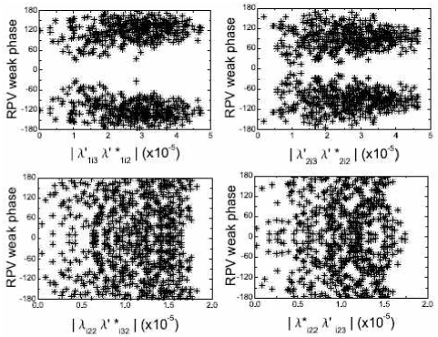
For the RPV couplings Ξ»i​11​λi​32β€²β£βˆ—subscriptπœ†π‘–11subscriptsuperscriptπœ†β€²π‘–32\lambda_{i11}\lambda^{\prime*}_{i32} and Ξ»i​11βˆ—β€‹Ξ»i​23β€²subscriptsuperscriptπœ†π‘–11subscriptsuperscriptπœ†β€²π‘–23\lambda^{*}_{i11}\lambda^{\prime}_{i23}, since their RPV weak phases are found to have very small contributions to the physical observables, we take their RPV weak phases to be free, and only give the upper limits for their modulus which are listed in Table IV. In Fig.3, we present our bounds on the other four RPV coupling products.
Refer to caption
Figure 3: The allowed parameter spaces for the relevant RPV coupling products constrained by the measurements listed in Table IV, and the RPV weak phase is given in degree.

From Fig.3, we find that every RPV weak phase are not constrained so much, but the modulus of the relevant RPV coupling products are tightly upper limited. The upper limits for the relevant RPV coupling products by Bβ†’K(βˆ—)​ℓ+β€‹β„“βˆ’β†’π΅superscript𝐾superscriptβ„“superscriptβ„“B\to K^{(*)}\ell^{+}\ell^{-} and Bsβ†’β„“+β€‹β„“βˆ’β†’subscript𝐡𝑠superscriptβ„“superscriptβ„“B_{s}\to\ell^{+}\ell^{-} decays are summarized in Table IV. For comparison, the existing bounds on these quadric coupling products [22, 30] are also listed. From Table IV, one can find that our bounds are more restrict than the previous ones. It’s also noted that the previous bounds of |Ξ»i​11​λi​32β€²β£βˆ—|subscriptπœ†π‘–11subscriptsuperscriptπœ†β€²π‘–32|\lambda_{i11}\lambda^{\prime*}_{i32}| and |Ξ»i​11βˆ—β€‹Ξ»i​23β€²|subscriptsuperscriptπœ†π‘–11subscriptsuperscriptπœ†β€²π‘–23|\lambda^{*}_{i11}\lambda^{\prime}_{i23}| are obtained at the MG​U​Tsubscriptπ‘€πΊπ‘ˆπ‘‡M_{GUT} scale in the RPV mSUGRA model [30].

Table IV: Bounds for the relevant RPV coupling products by Bβ†’K(βˆ—)​ℓ+β€‹β„“βˆ’β†’π΅superscript𝐾superscriptβ„“superscriptβ„“B\to K^{(*)}\ell^{+}\ell^{-} and Bsβ†’β„“+β€‹β„“βˆ’β†’subscript𝐡𝑠superscriptβ„“superscriptβ„“B_{s}\to\ell^{+}\ell^{-} decays for 100 G​e​V𝐺𝑒𝑉GeV sfermions, and previous bounds are listed for comparison.

Couplings Β Β Β Β Β Β Β Β Β Β Β Bounds [Processes] Previous bounds [Processes]
|Ξ»1​i​3′​λ1​i​2β€²β£βˆ—|subscriptsuperscriptπœ†β€²1𝑖3subscriptsuperscriptπœ†β€²1𝑖2|\lambda^{\prime}_{1i3}\lambda^{\prime*}_{1i2}| ≀4.7Γ—10βˆ’5​[Bβ†’K(βˆ—)​e+​eβˆ’]absent4.7superscript105delimited-[]→𝐡superscript𝐾superscript𝑒superscript𝑒\leq 4.7\times 10^{-5}~{}[B\to K^{(*)}e^{+}e^{-}] ≀9.6Γ—10βˆ’5​[Bβ†’K​e+​eβˆ’]absent9.6superscript105delimited-[]→𝐡𝐾superscript𝑒superscript𝑒{\leq 9.6\times 10^{-5}~{}[B\to Ke^{+}e^{-}}] [22]
|Ξ»i​11​λi​32β€²β£βˆ—|subscriptπœ†π‘–11subscriptsuperscriptπœ†β€²π‘–32|\lambda_{i11}\lambda^{\prime*}_{i32}| ≀2.3Γ—10βˆ’5​[Bβ†’K(βˆ—)​e+​eβˆ’]absent2.3superscript105delimited-[]→𝐡superscript𝐾superscript𝑒superscript𝑒\leq 2.3\times 10^{-5}~{}[B\to K^{(*)}e^{+}e^{-}] ≀1.5Γ—10βˆ’3absent1.5superscript103\leq 1.5\times 10^{-3} [30]
|Ξ»i​11βˆ—β€‹Ξ»i​23β€²|subscriptsuperscriptπœ†π‘–11subscriptsuperscriptπœ†β€²π‘–23|\lambda^{*}_{i11}\lambda^{\prime}_{i23}| ≀2.3Γ—10βˆ’5​[Bβ†’K(βˆ—)​e+​eβˆ’]absent2.3superscript105delimited-[]→𝐡superscript𝐾superscript𝑒superscript𝑒\leq 2.3\times 10^{-5}~{}[B\to K^{(*)}e^{+}e^{-}] ≀1.9Γ—10βˆ’4absent1.9superscript104\leq 1.9\times 10^{-4} [30]
|Ξ»2​i​3′​λ2​i​2β€²β£βˆ—|subscriptsuperscriptπœ†β€²2𝑖3subscriptsuperscriptπœ†β€²2𝑖2|\lambda^{\prime}_{2i3}\lambda^{\prime*}_{2i2}| ≀4.6Γ—10βˆ’5[Bβ†’K(βˆ—)​μ+β€‹ΞΌβˆ’][Bsβ†’ΞΌ+β€‹ΞΌβˆ’]\leq 4.6\times 10^{-5}~{}_{[B\to K^{(*)}\mu^{+}\mu^{-}]}^{[B_{s}\to\mu^{+}\mu^{-}]} ≀3.9Γ—10βˆ’3​[Bsβ†’ΞΌ+β€‹ΞΌβˆ’]≀9.7Γ—10βˆ’5​[Bβ†’K​μ+β€‹ΞΌβˆ’]superscriptsubscriptabsentabsent9.7superscript105delimited-[]→𝐡𝐾superscriptπœ‡superscriptπœ‡absent3.9superscript103delimited-[]β†’subscript𝐡𝑠superscriptπœ‡superscriptπœ‡{}_{\leq 9.7\times 10^{-5}~{}[B\to K\mu^{+}\mu^{-}]}^{\leq 3.9\times 10^{-3}~{}[B_{s}\to\mu^{+}\mu^{-}]} [22]
|Ξ»i​22​λi​32β€²β£βˆ—|subscriptπœ†π‘–22subscriptsuperscriptπœ†β€²π‘–32|\lambda_{i22}\lambda^{\prime*}_{i32}| ≀1.8Γ—10βˆ’5[Bβ†’K(βˆ—)​μ+β€‹ΞΌβˆ’][Bsβ†’ΞΌ+β€‹ΞΌβˆ’]\leq 1.8\times 10^{-5}~{}_{[B\to K^{(*)}\mu^{+}\mu^{-}]}^{[B_{s}\to\mu^{+}\mu^{-}]} ≀2.7Γ—10βˆ’5​[Bβ†’K​μ+β€‹ΞΌβˆ’]absent2.7superscript105delimited-[]→𝐡𝐾superscriptπœ‡superscriptπœ‡\leq 2.7\times 10^{-5}~{}[B\to K\mu^{+}\mu^{-}] [22]
|Ξ»i​22βˆ—β€‹Ξ»i​23β€²|subscriptsuperscriptπœ†π‘–22subscriptsuperscriptπœ†β€²π‘–23|\lambda^{*}_{i22}\lambda^{\prime}_{i23}| ≀1.7Γ—10βˆ’5[Bβ†’K(βˆ—)​μ+β€‹ΞΌβˆ’][Bsβ†’ΞΌ+β€‹ΞΌβˆ’]\leq 1.7\times 10^{-5}~{}_{[B\to K^{(*)}\mu^{+}\mu^{-}]}^{[B_{s}\to\mu^{+}\mu^{-}]} ≀2.7Γ—10βˆ’5​[Bβ†’K​μ+β€‹ΞΌβˆ’]absent2.7superscript105delimited-[]→𝐡𝐾superscriptπœ‡superscriptπœ‡\leq 2.7\times 10^{-5}~{}[B\to K\mu^{+}\mu^{-}] [22]

Using the constrained parameter spaces shown in Table IV and Fig.3, we can predict the RPV effects on the other quantities which have not been well measured yet in these processes. We perform a scan over the input parameters and the new constrained RPV coupling spaces to get the allowed ranges for ℬ​(Bsβ†’β„“+β€‹β„“βˆ’)ℬ→subscript𝐡𝑠superscriptβ„“superscriptβ„“\mathcal{B}(B_{s}\to\ell^{+}\ell^{-}) and π’œF​B​(Bβ†’K(βˆ—)​ℓ+β€‹β„“βˆ’)subscriptπ’œπΉπ΅β†’π΅superscript𝐾superscriptβ„“superscriptβ„“\mathcal{A}_{FB}(B\to K^{(*)}\ell^{+}\ell^{-}) with the different RPV coupling products. Our numerical results are summarized in Table V.

Table V: The theoretical predictions for ℬ​(Bsβ†’β„“+β€‹β„“βˆ’)ℬ→subscript𝐡𝑠superscriptβ„“superscriptβ„“\mathcal{B}(B_{s}\to\ell^{+}\ell^{-}) and π’œF​B​(Bβ†’K(βˆ—)​ℓ+β€‹β„“βˆ’)subscriptπ’œπΉπ΅β†’π΅superscript𝐾superscriptβ„“superscriptβ„“\mathcal{A}_{FB}(B\to K^{(*)}\ell^{+}\ell^{-}) in the SM and the RPV SUSY. The RPV SUSY predictions are obtained by the constrained regions of the different RPV coupling products. The index g=1𝑔1g=1 and 222 for β„“=eℓ𝑒\ell=e and ΞΌπœ‡\mu, respectively.

SM value Ξ»g​i​3′​λg​i​2β€²β£βˆ—subscriptsuperscriptπœ†β€²π‘”π‘–3subscriptsuperscriptπœ†β€²π‘”π‘–2\lambda^{\prime}_{gi3}\lambda^{\prime*}_{gi2} Ξ»i​g​g​λi​32β€²β£βˆ—subscriptπœ†π‘–π‘”π‘”subscriptsuperscriptπœ†β€²π‘–32\lambda_{igg}\lambda^{\prime*}_{i32} Ξ»i​g​gβˆ—β€‹Ξ»i​23β€²subscriptsuperscriptπœ†π‘–π‘”π‘”subscriptsuperscriptπœ†β€²π‘–23\lambda^{*}_{igg}\lambda^{\prime}_{i23}
ℬ​(Bsβ†’e+​eβˆ’)ℬ→subscript𝐡𝑠superscript𝑒superscript𝑒\mathcal{B}(B_{s}\to e^{+}e^{-}) [5.9,11.2]Γ—10βˆ’145.911.2superscript1014[5.9,11.2]\times 10^{-14} [5.3,17.0]Γ—10βˆ’145.317.0superscript1014[5.3,17.0]\times 10^{-14} ≀2.2Γ—10βˆ’7absent2.2superscript107\leq 2.2\times 10^{-7} ≀2.2Γ—10βˆ’7absent2.2superscript107\leq 2.2\times 10^{-7}
π’œF​B​(Bβ†’K​e+​eβˆ’)subscriptπ’œπΉπ΅β†’π΅πΎsuperscript𝑒superscript𝑒\mathcal{A}_{FB}(B\to Ke^{+}e^{-}) 00 00 [βˆ’4.1,5.0]Γ—10βˆ’54.15.0superscript105[-4.1,5.0]\times 10^{-5} [βˆ’4.0,5.0]Γ—10βˆ’54.05.0superscript105[-4.0,5.0]\times 10^{-5}
π’œF​B​(Bβ†’Kβˆ—β€‹e+​eβˆ’)subscriptπ’œπΉπ΅β†’π΅superscript𝐾superscript𝑒superscript𝑒\mathcal{A}_{FB}(B\to K^{*}e^{+}e^{-}) [0.12,0.18]0.120.18[0.12,0.18] [0.00,0.29]0.000.29[0.00,0.29] [0.12,0.18]0.120.18[0.12,0.18] [0.13,0.18]0.130.18[0.13,0.18]
ℬ​(Bsβ†’ΞΌ+β€‹ΞΌβˆ’)ℬ→subscript𝐡𝑠superscriptπœ‡superscriptπœ‡\mathcal{B}(B_{s}\to\mu^{+}\mu^{-}) [2.7,4.8]Γ—10βˆ’92.74.8superscript109[2.7,4.8]\times 10^{-9} [2.1,6.8]Γ—10βˆ’92.16.8superscript109[2.1,6.8]\times 10^{-9} <1.0Γ—10βˆ’7absent1.0superscript107<1.0\times 10^{-7} <1.0Γ—10βˆ’7absent1.0superscript107<1.0\times 10^{-7}
π’œF​B​(Bβ†’K​μ+β€‹ΞΌβˆ’)subscriptπ’œπΉπ΅β†’π΅πΎsuperscriptπœ‡superscriptπœ‡\mathcal{A}_{FB}(B\to K\mu^{+}\mu^{-}) 00 00 [βˆ’7.0,6.9]Γ—10βˆ’37.06.9superscript103[-7.0,6.9]\times 10^{-3} [βˆ’6.8,7.0]Γ—10βˆ’36.87.0superscript103[-6.8,7.0]\times 10^{-3}
π’œF​B​(Bβ†’Kβˆ—β€‹ΞΌ+β€‹ΞΌβˆ’)subscriptπ’œπΉπ΅β†’π΅superscript𝐾superscriptπœ‡superscriptπœ‡\mathcal{A}_{FB}(B\to K^{*}\mu^{+}\mu^{-}) [0.13,0.18]0.130.18[0.13,0.18] [0.02,0.76]0.020.76[0.02,0.76] [0.13,0.18]0.130.18[0.13,0.18] [0.13,0.18]0.130.18[0.13,0.18]

From the Table V, we can find some salient features of the numerical results.

  • β€’

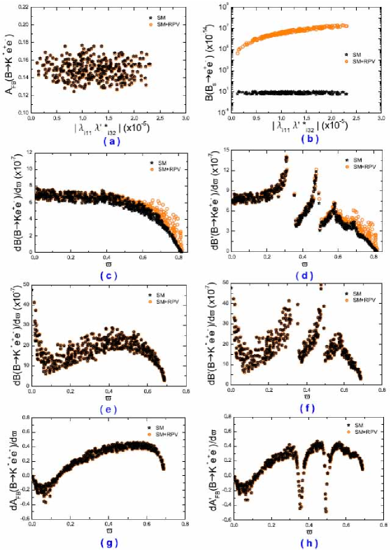
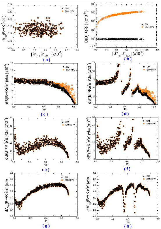
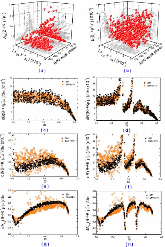
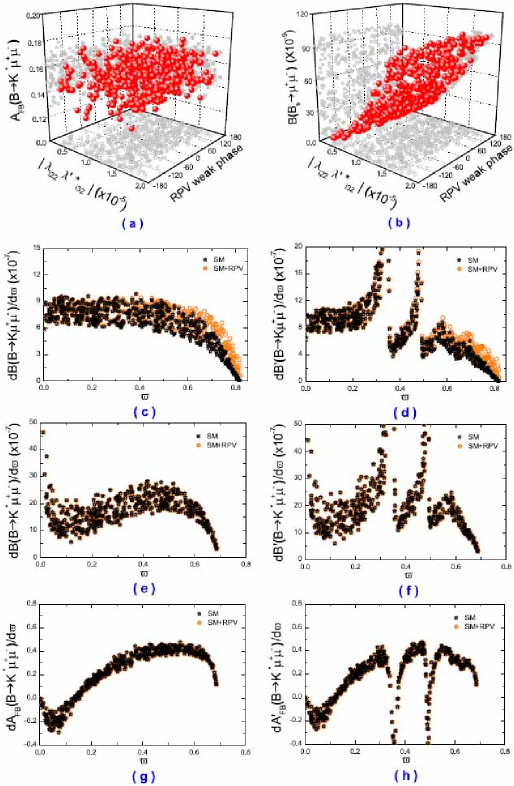
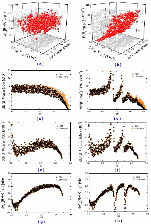
    I. As shown by Fig.2(b), the contributions of Ξ»1​i​3′​λ1​i​2β€²β£βˆ—subscriptsuperscriptπœ†β€²1𝑖3subscriptsuperscriptπœ†β€²1𝑖2\lambda^{\prime}_{1i3}\lambda^{\prime*}_{1i2} and Ξ»2​i​3′​λ2​i​2β€²β£βˆ—subscriptsuperscriptπœ†β€²2𝑖3subscriptsuperscriptπœ†β€²2𝑖2\lambda^{\prime}_{2i3}\lambda^{\prime*}_{2i2} to ℬ​(Bsβ†’e+​eβˆ’)ℬ→subscript𝐡𝑠superscript𝑒superscript𝑒\mathcal{B}(B_{s}\to e^{+}e^{-}) and ℬ​(Bsβ†’ΞΌ+β€‹ΞΌβˆ’)ℬ→subscript𝐡𝑠superscriptπœ‡superscriptπœ‡\mathcal{B}(B_{s}\to\mu^{+}\mu^{-}), respectively, arise from t-channel squark exchange . After Fierz transformation, the effective Hamiltonian due to the t-channel squark exchange is proportional to (s¯​γμ​PR​b)​(ℓ¯​γμ​PL​ℓ)¯𝑠superscriptπ›Ύπœ‡subscript𝑃𝑅𝑏¯ℓsubscriptπ›Ύπœ‡subscript𝑃𝐿ℓ\Big{(}\bar{s}\gamma^{\mu}P_{R}b\Big{)}\Big{(}\bar{\ell}\gamma_{\mu}P_{L}\ell\Big{)}, which contribution to ℬ​(Bsβ†’β„“+β€‹β„“βˆ’)ℬ→subscript𝐡𝑠superscriptβ„“superscriptβ„“\mathcal{B}(B_{s}\to\ell^{+}\ell^{-}) is suppressed by mβ„“2/mB2subscriptsuperscriptπ‘š2β„“subscriptsuperscriptπ‘š2𝐡m^{2}_{\ell}/m^{2}_{B} due to helicity suppression. Therefore ℬ​(Bsβ†’e+​eβˆ’,ΞΌ+β€‹ΞΌβˆ’)ℬ→subscript𝐡𝑠superscript𝑒superscript𝑒superscriptπœ‡superscriptπœ‡\mathcal{B}(B_{s}\to e^{+}e^{-},\mu^{+}\mu^{-}) will not be enhanced so much by the t-channel squark exchanging RPV contributions. However, the effective Hamiltonian of s-channel sneutrino exchange would be (s¯​(1Β±Ξ³5)​b)​(ℓ¯​(1βˆ“Ξ³5)​ℓ)¯𝑠plus-or-minus1subscript𝛾5𝑏¯ℓminus-or-plus1subscript𝛾5β„“\Big{(}\bar{s}(1\pm\gamma_{5})b\Big{)}\Big{(}\bar{\ell}(1\mp\gamma_{5})\ell\Big{)}, which contributions are not suppressed by mβ„“2/mB2subscriptsuperscriptπ‘š2β„“subscriptsuperscriptπ‘š2𝐡m^{2}_{\ell}/m^{2}_{B}. So that, both ℬ​(Bsβ†’e+​eβˆ’)ℬ→subscript𝐡𝑠superscript𝑒superscript𝑒\mathcal{B}(B_{s}\to e^{+}e^{-}) and ℬ​(Bsβ†’ΞΌ+β€‹ΞΌβˆ’)ℬ→subscript𝐡𝑠superscriptπœ‡superscriptπœ‡\mathcal{B}(B_{s}\to\mu^{+}\mu^{-}) could be enhanced to order 10βˆ’7superscript10710^{-7} by Ξ»i​11​λi​32β€²β£βˆ—β€‹(Ξ»i​11βˆ—β€‹Ξ»i​23β€²)subscriptπœ†π‘–11superscriptsubscriptπœ†π‘–32β€²subscriptsuperscriptπœ†π‘–11subscriptsuperscriptπœ†β€²π‘–23\lambda_{i11}\lambda_{i32}^{\prime*}(\lambda^{*}_{i11}\lambda^{\prime}_{i23}) and Ξ»i​22​λi​32β€²β£βˆ—β€‹(Ξ»i​22βˆ—β€‹Ξ»i​23β€²)subscriptπœ†π‘–22superscriptsubscriptπœ†π‘–32β€²subscriptsuperscriptπœ†π‘–22subscriptsuperscriptπœ†β€²π‘–23\lambda_{i22}\lambda_{i32}^{\prime*}(\lambda^{*}_{i22}\lambda^{\prime}_{i23}), respectively.

  • β€’

    II. Both π’œF​B​(Bβ†’K​e+​eβˆ’)subscriptπ’œπΉπ΅β†’π΅πΎsuperscript𝑒superscript𝑒\mathcal{A}_{FB}(B\to Ke^{+}e^{-}) and π’œF​B​(Bβ†’K​μ+β€‹ΞΌβˆ’)subscriptπ’œπΉπ΅β†’π΅πΎsuperscriptπœ‡superscriptπœ‡\mathcal{A}_{FB}(B\to K\mu^{+}\mu^{-}) are zero in the SM. The RPV contributions to the asymmetries due to squark exchange are also zero, while the sneutino exchange RPV contributions are too small to be accessible at LHC.

  • β€’

    III. It is interesting to note that the RPV squark exchange contributions have significant impacts on π’œF​B​(Bβ†’Kβˆ—β€‹e+​eβˆ’)subscriptπ’œπΉπ΅β†’π΅superscript𝐾superscript𝑒superscript𝑒\mathcal{A}_{FB}(B\to K^{*}e^{+}e^{-}) and π’œF​B​(Bβ†’Kβˆ—β€‹ΞΌ+β€‹ΞΌβˆ’)subscriptπ’œπΉπ΅β†’π΅superscript𝐾superscriptπœ‡superscriptπœ‡\mathcal{A}_{FB}(B\to K^{*}\mu^{+}\mu^{-}). However, the sneutrino exchange have negligible effects on π’œF​B​(Bβ†’Kβˆ—β€‹e+​eβˆ’)subscriptπ’œπΉπ΅β†’π΅superscript𝐾superscript𝑒superscript𝑒\mathcal{A}_{FB}(B\to K^{*}e^{+}e^{-}) and π’œF​B​(Bβ†’Kβˆ—β€‹ΞΌ+β€‹ΞΌβˆ’)subscriptπ’œπΉπ΅β†’π΅superscript𝐾superscriptπœ‡superscriptπœ‡\mathcal{A}_{FB}(B\to K^{*}\mu^{+}\mu^{-}).

Recently, the BABAR Collaboration [1] has measured

π’œF​B​(B+β†’K+​ℓ+β€‹β„“βˆ’)(s>0.1​G​e​V2)=0.15βˆ’0.23+0.21Β±0.08,subscriptπ’œπΉπ΅subscriptβ†’superscript𝐡superscript𝐾superscriptβ„“superscriptℓ𝑠0.1𝐺𝑒superscript𝑉2plus-or-minussubscriptsuperscript0.150.210.230.08\displaystyle\mathcal{A}_{FB}(B^{+}\to K^{+}\ell^{+}\ell^{-})_{(s>0.1GeV^{2})}=0.15^{+0.21}_{-0.23}\pm 0.08, (63)
π’œF​B(Bβ†’Kβˆ—β„“+β„“βˆ’)(s>0.1​G​e​V2)β‰₯0.55(95%C.L.),\displaystyle\mathcal{A}_{FB}(B\to K^{*}\ell^{+}\ell^{-})_{(s>0.1GeV^{2})}\geq 0.55~{}~{}(95\%C.L.), (64)

and Belle Collaboration has measured the integrated forward-backward asymmetries π’œ~F​Bsubscript~π’œπΉπ΅\widetilde{\mathcal{A}}_{FB} [3]

π’œ~F​B​(B+β†’K+​ℓ+β€‹β„“βˆ’)=0.10Β±0.14Β±0.01,subscript~π’œπΉπ΅β†’superscript𝐡superscript𝐾superscriptβ„“superscriptβ„“plus-or-minus0.100.140.01\displaystyle\widetilde{\mathcal{A}}_{FB}(B^{+}\to K^{+}\ell^{+}\ell^{-})=0.10\pm 0.14\pm 0.01, (65)
π’œ~F​B​(Bβ†’Kβˆ—β€‹β„“+β€‹β„“βˆ’)=0.50Β±0.15Β±0.02,subscript~π’œπΉπ΅β†’π΅superscript𝐾superscriptβ„“superscriptβ„“plus-or-minus0.500.150.02\displaystyle\widetilde{\mathcal{A}}_{FB}(B\to K^{*}\ell^{+}\ell^{-})=0.50\pm 0.15\pm 0.02, (66)

where π’œ~F​Bsubscript~π’œπΉπ΅\widetilde{\mathcal{A}}_{FB} is slightly different from π’œF​Bsubscriptπ’œπΉπ΅\mathcal{A}_{FB}, and defined by

π’œ~F​B​(Bβ†’K(βˆ—)​ℓ+β€‹β„“βˆ’)=∫d2​ℬ​(Bβ†’K(βˆ—)​ℓ+β€‹β„“βˆ’)d​c​o​s​θ​d​s^​s​i​g​n​(c​o​s​θ)​𝑑c​o​s​θ​𝑑s^∫d2​ℬ​(Bβ†’K(βˆ—)​ℓ+β€‹β„“βˆ’)d​c​o​s​θ​d​s^​𝑑c​o​s​θ​𝑑s^.subscript~π’œπΉπ΅β†’π΅superscript𝐾superscriptβ„“superscriptβ„“superscript𝑑2ℬ→𝐡superscript𝐾superscriptβ„“superscriptβ„“π‘‘π‘π‘œπ‘ πœƒπ‘‘^π‘ π‘ π‘–π‘”π‘›π‘π‘œπ‘ πœƒdifferential-dπ‘π‘œπ‘ πœƒdifferential-d^𝑠superscript𝑑2ℬ→𝐡superscript𝐾superscriptβ„“superscriptβ„“π‘‘π‘π‘œπ‘ πœƒπ‘‘^𝑠differential-dπ‘π‘œπ‘ πœƒdifferential-d^𝑠\displaystyle\widetilde{\mathcal{A}}_{FB}(B\to K^{(*)}\ell^{+}\ell^{-})=\frac{\int\frac{d^{2}\mathcal{B}(B\to K^{(*)}\ell^{+}\ell^{-})}{dcos\theta d\hat{s}}sign(cos\theta)dcos\theta d\hat{s}}{\int\frac{d^{2}\mathcal{B}(B\to K^{(*)}\ell^{+}\ell^{-})}{dcos\theta d\hat{s}}dcos\theta d\hat{s}}. (67)

We find that the SM predictions for π’œF​B​(Bβ†’Kβˆ—β€‹β„“+β€‹β„“βˆ’)subscriptπ’œπΉπ΅β†’π΅superscript𝐾superscriptβ„“superscriptβ„“\mathcal{A}_{FB}(B\to K^{*}\ell^{+}\ell^{-}) are consistent with both the measurements within error bars.

In Figs.4-9, we present correlations between the physical observable ℬℬ\mathcal{B}, π’œF​Bsubscriptπ’œπΉπ΅\mathcal{A}_{FB} and the parameter spaces of the different RPV coupling products by the three-dimensional scatter plots and the two-dimensional scatter plots, respectively. The dilepton invariant mass distribution and the normalized forward-backward asymmetry are given with VMD contribution excluded in terms of d​ℬ/d​s^𝑑ℬ𝑑^𝑠d\mathcal{B}/d\hat{s} and dβ€‹π’œF​B/d​s^𝑑subscriptπ’œπΉπ΅π‘‘^𝑠d\mathcal{A}_{FB}/d\hat{s}, and included in d​ℬ′/d​s^𝑑superscriptℬ′𝑑^𝑠d\mathcal{B}^{\prime}/d\hat{s} and dβ€‹π’œF​Bβ€²/d​s^𝑑subscriptsuperscriptπ’œβ€²πΉπ΅π‘‘^𝑠d\mathcal{A}^{\prime}_{FB}/d\hat{s}, respectively. From Figs.4-9, one can find the correlations of these physical observables with RPV coupling products. In Figs.5-6, since the influences of the RPV weak phases are very small, we take the RPV weak phases randomly varied in [βˆ’Ο€,Ο€]πœ‹πœ‹[-\pi,\pi] and only give the change trends of the physical observables with the relative modulus in the two-dimensional scatter plots.

At first, we will discuss plots of Fig.4 in detail. The three-dimensional scatter plot Fig.4(a) shows π’œF​B​(Bβ†’Kβˆ—β€‹e+​eβˆ’)subscriptπ’œπΉπ΅β†’π΅superscript𝐾superscript𝑒superscript𝑒\mathcal{A}_{FB}(B\to K^{*}e^{+}e^{-}) correlated with |Ξ»1​i​3′​λ1​i​2β€²β£βˆ—|subscriptsuperscriptπœ†β€²1𝑖3subscriptsuperscriptπœ†β€²1𝑖2|\lambda^{\prime}_{1i3}\lambda^{\prime*}_{1i2}| and its phase ϕ​Rpsubscriptitalic-Ο•subscript𝑅𝑝\phi_{\not\!R_{p}\,}. We also give projections on three vertical planes, where the |Ξ»1​i​3′​λ1​i​2β€²β£βˆ—|subscriptsuperscriptπœ†β€²1𝑖3subscriptsuperscriptπœ†β€²1𝑖2|\lambda^{\prime}_{1i3}\lambda^{\prime*}_{1i2}|-ϕ​Rpsubscriptitalic-Ο•subscript𝑅𝑝\phi_{\not\!R_{p}\,} plane displays the constrained regions of Ξ»1​i​3′​λ1​i​2β€²β£βˆ—subscriptsuperscriptπœ†β€²1𝑖3subscriptsuperscriptπœ†β€²1𝑖2\lambda^{\prime}_{1i3}\lambda^{\prime*}_{1i2} as the first plot of Fig.3. It’s shown that π’œF​B​(Bβ†’Kβˆ—β€‹e+​eβˆ’)subscriptπ’œπΉπ΅β†’π΅superscript𝐾superscript𝑒superscript𝑒\mathcal{A}_{FB}(B\to K^{*}e^{+}e^{-}) is decreasing with |Ξ»1​i​3′​λ1​i​2β€²β£βˆ—|subscriptsuperscriptπœ†β€²1𝑖3subscriptsuperscriptπœ†β€²1𝑖2|\lambda^{\prime}_{1i3}\lambda^{\prime*}_{1i2}| on the π’œF​B​(Bβ†’Kβˆ—β€‹e+​eβˆ’)subscriptπ’œπΉπ΅β†’π΅superscript𝐾superscript𝑒superscript𝑒\mathcal{A}_{FB}(B\to K^{*}e^{+}e^{-})-|Ξ»1​i​3′​λ1​i​2β€²β£βˆ—|subscriptsuperscriptπœ†β€²1𝑖3subscriptsuperscriptπœ†β€²1𝑖2|\lambda^{\prime}_{1i3}\lambda^{\prime*}_{1i2}| plane. From the π’œF​B​(Bβ†’Kβˆ—β€‹e+​eβˆ’)subscriptπ’œπΉπ΅β†’π΅superscript𝐾superscript𝑒superscript𝑒\mathcal{A}_{FB}(B\to K^{*}e^{+}e^{-})-ϕ​Rpsubscriptitalic-Ο•subscript𝑅𝑝\phi_{\not\!R_{p}\,} plane, we can see that π’œF​B​(Bβ†’Kβˆ—β€‹e+​eβˆ’)subscriptπ’œπΉπ΅β†’π΅superscript𝐾superscript𝑒superscript𝑒\mathcal{A}_{FB}(B\to K^{*}e^{+}e^{-}) is decreasing with |ϕ​Rp|subscriptitalic-Ο•subscript𝑅𝑝|\phi_{\not\!R_{p}\,}|. The recent measurement of π’œF​B​(Bβ†’Kβˆ—β€‹β„“+β€‹β„“βˆ’)subscriptπ’œπΉπ΅β†’π΅superscript𝐾superscriptβ„“superscriptβ„“\mathcal{A}_{FB}(B\to K^{*}\ell^{+}\ell^{-}) favors |Ξ»1​i​3′​λ1​i​2β€²β£βˆ—|subscriptsuperscriptπœ†β€²1𝑖3subscriptsuperscriptπœ†β€²1𝑖2|\lambda^{\prime}_{1i3}\lambda^{\prime*}_{1i2}|∼(2∼4)Γ—10βˆ’5similar-toabsentsimilar-to24superscript105\sim(2\sim 4)\times 10^{-5} with small ϕ​Rpsubscriptitalic-Ο•subscript𝑅𝑝\phi_{\not\!R_{p}\,}. However Bsβ†’e+​eβˆ’β†’subscript𝐡𝑠superscript𝑒superscript𝑒B_{s}\to e^{+}e^{-} is remained inaccessible at LHC. From plots Fig.4(c-h), we can find that the theoretical uncertainties in the calculation of the SM contributions are still very large, nevertheless, for d​ℬ​(Bβ†’K(βˆ—)​e+​eβˆ’)/d​s^𝑑ℬ→𝐡superscript𝐾superscript𝑒superscript𝑒𝑑^𝑠d\mathcal{B}(B\to K^{(*)}e^{+}e^{-})/d\hat{s} and dβ€‹π’œF​B​(Bβ†’Kβˆ—β€‹e+​eβˆ’)/d​s^𝑑subscriptπ’œπΉπ΅β†’π΅superscript𝐾superscript𝑒superscript𝑒𝑑^𝑠d\mathcal{A}_{FB}(B\to K^{*}e^{+}e^{-})/d\hat{s}, the Ξ»1​i​3′​λ1​i​2β€²β£βˆ—subscriptsuperscriptπœ†β€²1𝑖3subscriptsuperscriptπœ†β€²1𝑖2\lambda^{\prime}_{1i3}\lambda^{\prime*}_{1i2} contributions are distinguishable from the hadronic uncertainties.

Fig.5 and Fig.6 are the contributions of Ξ»i​11​λi​32β€²β£βˆ—subscriptπœ†π‘–11subscriptsuperscriptπœ†β€²π‘–32\lambda_{i11}\lambda^{\prime*}_{i32} and Ξ»i​11βˆ—β€‹Ξ»i​23β€²subscriptsuperscriptπœ†π‘–11subscriptsuperscriptπœ†β€²π‘–23\lambda^{*}_{i11}\lambda^{\prime}_{i23}, respectively. It is interesting to note that the t-channel RPV sneutrino exchange could enhance ℬ​(Bsβ†’e+​eβˆ’)ℬ→subscript𝐡𝑠superscript𝑒superscript𝑒\mathcal{B}(B_{s}\to e^{+}e^{-}) by about 6 orders of magnitude (Fig.5(b) and Fig.6(b)). Moreover, they could give distinguishable contributions to d​ℬ​(Bβ†’K​e+​eβˆ’)/d​s^𝑑ℬ→𝐡𝐾superscript𝑒superscript𝑒𝑑^𝑠d\mathcal{B}(B\to Ke^{+}e^{-})/d\hat{s} in the high s^^𝑠\hat{s} region. For other observables, their contributions are indistinguishable from hadronic uncertainties.

The RPV squark exchange contributions to Bβ†’K(βˆ—)​μ+β€‹ΞΌβˆ’β†’π΅superscript𝐾superscriptπœ‡superscriptπœ‡B\to K^{(*)}\mu^{+}\mu^{-} and Bsβ†’ΞΌ+β€‹ΞΌβˆ’β†’subscript𝐡𝑠superscriptπœ‡superscriptπœ‡B_{s}\to\mu^{+}\mu^{-} are presented in Fig.7. Such contributions could give large π’œF​B​(Bβ†’Kβˆ—β€‹ΞΌ+β€‹ΞΌβˆ’)subscriptπ’œπΉπ΅β†’π΅superscript𝐾superscriptπœ‡superscriptπœ‡\mathcal{A}_{FB}(B\to K^{*}\mu^{+}\mu^{-}) in favor of Belle and BABAR measurements, however, small corrections to ℬ​(Bsβ†’ΞΌ+β€‹ΞΌβˆ’)ℬ→subscript𝐡𝑠superscriptπœ‡superscriptπœ‡\mathcal{B}(B_{s}\to\mu^{+}\mu^{-}).

The RPV sneutrino exchange contributions to Bβ†’Kβˆ—β€‹ΞΌ+β€‹ΞΌβˆ’β†’π΅superscript𝐾superscriptπœ‡superscriptπœ‡B\to K^{*}\mu^{+}\mu^{-} and Bsβ†’ΞΌ+β€‹ΞΌβˆ’β†’subscript𝐡𝑠superscriptπœ‡superscriptπœ‡B_{s}\to\mu^{+}\mu^{-} are displayed in Fig.8 and Fig.9, respectively. From plots in these two figures, we find ℬ​(Bsβ†’ΞΌ+β€‹ΞΌβˆ’)ℬ→subscript𝐡𝑠superscriptπœ‡superscriptπœ‡\mathcal{B}(B_{s}\to\mu^{+}\mu^{-}) is very sensitive to such contributions. Within the constrained parameter space for Ξ»i​22​λi​32β€²β£βˆ—subscriptπœ†π‘–22subscriptsuperscriptπœ†β€²π‘–32\lambda_{i22}\lambda^{\prime*}_{i32} and Ξ»i​22βˆ—β€‹Ξ»i​23β€²subscriptsuperscriptπœ†π‘–22subscriptsuperscriptπœ†β€²π‘–23\lambda^{*}_{i22}\lambda^{\prime}_{i23}, RPV contributions can enhance ℬ​(Bsβ†’ΞΌ+β€‹ΞΌβˆ’)ℬ→subscript𝐡𝑠superscriptπœ‡superscriptπœ‡\mathcal{B}(B_{s}\to\mu^{+}\mu^{-}) by two orders, which could be accessible at LHC and Tevatron in the forthcoming years. We also note that these contributions to other observables are small, regarding to the large theoretical uncertainties.

It is worth to note that, in the BABAR measurement[1], the value of π’œF​B​(Bβ†’Kβˆ—β€‹β„“+β€‹β„“βˆ’)subscriptπ’œπΉπ΅β†’π΅superscript𝐾superscriptβ„“superscriptβ„“\mathcal{A}_{FB}(B\to K^{*}\ell^{+}\ell^{-}) with 95%​C.L.percent95C.L.95\%~{}\emph{C.L.} lower limit is slightly above the SM prediction in low s^^𝑠\hat{s} region. We have found that the RPV couplings Ξ»1​i​3′​λ1​i​2β€²β£βˆ—subscriptsuperscriptπœ†β€²1𝑖3subscriptsuperscriptπœ†β€²1𝑖2\lambda^{\prime}_{1i3}\lambda^{\prime*}_{1i2} and Ξ»2​i​3′​λ2​i​2β€²β£βˆ—subscriptsuperscriptπœ†β€²2𝑖3subscriptsuperscriptπœ†β€²2𝑖2\lambda^{\prime}_{2i3}\lambda^{\prime*}_{2i2} could enhance π’œF​B​(Bβ†’Kβˆ—β€‹β„“+β€‹β„“βˆ’)subscriptπ’œπΉπ΅β†’π΅superscript𝐾superscriptβ„“superscriptβ„“\mathcal{A}_{FB}(B\to K^{*}\ell^{+}\ell^{-}) to accommodate the possible discrepancy, which are shown by the following Fig.4(g) and Fig.7(g), respectively.

Generally, the predictions of B𝐡B decays suffer from many theoretical uncertainties. Recently, beyond naive factorization, Bβ†’Kβˆ—β†’π΅superscriptπΎβˆ—B\to K^{\ast} have been investigated with the QCD factorization[31] framework in [32, 33], and then studied with Soft Collinear Effective Theory (SCET) [34] in Ref.[35]. However, the power corrections are found to be associated with large theoretical uncertainties, and we are conservative to the naive factorization in this paper.

To probe new physics effects, it would be very useful to measure correlative observables, for example, dβ€‹π’œF​B​(Bβ†’Kβˆ—β€‹ΞΌ+β€‹ΞΌβˆ’)/d​s^𝑑subscriptπ’œπΉπ΅β†’π΅superscript𝐾superscriptπœ‡superscriptπœ‡π‘‘^𝑠d\mathcal{A}_{FB}(B\to K^{*}\mu^{+}\mu^{-})/d\hat{s}, d​ℬ​(Bβ†’Kβˆ—β€‹ΞΌ+β€‹ΞΌβˆ’)/d​s^𝑑ℬ→𝐡superscript𝐾superscriptπœ‡superscriptπœ‡π‘‘^𝑠d\mathcal{B}(B\to K^{*}\mu^{+}\mu^{-})/d\hat{s} and ℬ​(Bsβ†’ΞΌ+β€‹ΞΌβˆ’)ℬ→subscript𝐡𝑠superscriptπœ‡superscriptπœ‡\mathcal{B}(B_{s}\to\mu^{+}\mu^{-}), since correlations among these observables could provide very strict bound on new physics models. At present, one may have to wait for the error bars in the measurements of these observables to come down and more channels to be measured. With the operation of B𝐡B factory experiments, large amounts of experimental data on hadronic B𝐡B meson decays are being collected, and measurements of previously known observable will become more precise. From the comparison of our predictions in Figs.4-9 with the near future experiments, one will obtain more stringent bounds on the products of RPV couplings. On the other hand, the RPV SUSY predictions of other decays will become more precise by the more stringent bounds on the RPV couplings.

4 Conclusions

In conclusion, the decays Bβ†’K(βˆ—)​ℓ+β€‹β„“βˆ’β†’π΅superscript𝐾superscriptβ„“superscriptβ„“B\to K^{(*)}\ell^{+}\ell^{-} and Bsβ†’β„“+β€‹β„“βˆ’β†’subscript𝐡𝑠superscriptβ„“superscriptβ„“B_{s}\to\ell^{+}\ell^{-} are very promising means to probe effects of new physics scenarios. In this paper, we have studied the Bβ†’K(βˆ—)​ℓ+β€‹β„“βˆ’β†’π΅superscript𝐾superscriptβ„“superscriptβ„“B\to K^{(*)}\ell^{+}\ell^{-} and Bsβ†’β„“+β€‹β„“βˆ’β†’subscript𝐡𝑠superscriptβ„“superscriptβ„“B_{s}\to\ell^{+}\ell^{-} decays in the RPV SUSY model. We have obtained fairly constrained parameter spaces of the RPV coupling products from the present experimental data of Bβ†’K(βˆ—)​ℓ+β€‹β„“βˆ’β†’π΅superscript𝐾superscriptβ„“superscriptβ„“B\to K^{(*)}\ell^{+}\ell^{-} and Bsβ†’β„“+β€‹β„“βˆ’β†’subscript𝐡𝑠superscriptβ„“superscriptβ„“B_{s}\to\ell^{+}\ell^{-} decays, and found these constraints are stronger than the existing ones, which may be useful for further studies of the RPV SUSY phenomenology. Furthermore, using the constrained parameter spaces, we have presented the RPV effects on the forward-backward asymmetries of Bβ†’K(βˆ—)​ℓ+β€‹β„“βˆ’β†’π΅superscript𝐾superscriptβ„“superscriptβ„“B\to K^{(*)}\ell^{+}\ell^{-} and the branching ratios of the pure leptonic Bssubscript𝐡𝑠B_{s} decays. Our results of π’œF​B​(Bβ†’K(βˆ—)​ℓ+β€‹β„“βˆ’)subscriptπ’œπΉπ΅β†’π΅superscript𝐾superscriptβ„“superscriptβ„“\mathcal{A}_{FB}(B\to K^{(*)}\ell^{+}\ell^{-}) agree with the recent experimental data. It is shown that ℬ​(Bsβ†’β„“+β€‹β„“βˆ’)ℬ→subscript𝐡𝑠superscriptβ„“superscriptβ„“\mathcal{B}(B_{s}\to\ell^{+}\ell^{-}) could be enhanced several orders by the RPV couplings from the sneutrino exchange. Since we have poorly experimental information about the pure leptonic decay Bsβ†’β„“+β€‹β„“βˆ’β†’subscript𝐡𝑠superscriptβ„“superscriptβ„“B_{s}\to\ell^{+}\ell^{-}, further refined measurements of ℬ​(Bsβ†’β„“+β€‹β„“βˆ’)ℬ→subscript𝐡𝑠superscriptβ„“superscriptβ„“\mathcal{B}(B_{s}\to\ell^{+}\ell^{-}) can further restrict the constrained space of the four RPV couplings from the sneutrino exchange. We have also compared the SM predictions with the RPV predictions about dilepton invariant mass spectra and the normalized forward-backward asymmetries in Bβ†’K(βˆ—)​ℓ+β€‹β„“βˆ’β†’π΅superscript𝐾superscriptβ„“superscriptβ„“B\to K^{(*)}\ell^{+}\ell^{-} decays. We have found that d​ℬ​(Bβ†’K​e+​eβˆ’)/d​s^𝑑ℬ→𝐡𝐾superscript𝑒superscript𝑒𝑑^𝑠d\mathcal{B}(B\to Ke^{+}e^{-})/d\hat{s} could be mildly decreased by the RPV coupling Ξ»1​i​3′​λ1​i​2β€²β£βˆ—subscriptsuperscriptπœ†β€²1𝑖3subscriptsuperscriptπœ†β€²1𝑖2\lambda^{\prime}_{1i3}\lambda^{\prime*}_{1i2}, and the Ξ»2​i​3′​λ2​i​2β€²β£βˆ—subscriptsuperscriptπœ†β€²2𝑖3subscriptsuperscriptπœ†β€²2𝑖2\lambda^{\prime}_{2i3}\lambda^{\prime*}_{2i2} contributions to d​ℬ​(Bβ†’K​μ+β€‹ΞΌβˆ’)/d​s^𝑑ℬ→𝐡𝐾superscriptπœ‡superscriptπœ‡π‘‘^𝑠d\mathcal{B}(B\to K\mu^{+}\mu^{-})/d\hat{s} are indistinguishable from the hadronic uncertainties. The other four RPV couplings due to the sneutrino exchange have distinguishable effects on d​ℬ​(Bβ†’K​ℓ+β€‹β„“βˆ’)/d​s^𝑑ℬ→𝐡𝐾superscriptβ„“superscriptℓ𝑑^𝑠d\mathcal{B}(B\to K\ell^{+}\ell^{-})/d\hat{s} at high s^^𝑠\hat{s}. For the Bβ†’Kβˆ—β€‹β„“+β€‹β„“βˆ’β†’π΅superscript𝐾superscriptβ„“superscriptβ„“B\to K^{*}\ell^{+}\ell^{-} decays, the squark exchange contributions have distinguishable effects on d​ℬ/d​s^𝑑ℬ𝑑^𝑠d\mathcal{B}/d\hat{s} and dβ€‹π’œF​B/d​s^𝑑subscriptπ’œπΉπ΅π‘‘^𝑠d\mathcal{A}_{FB}/d\hat{s}, but the contributions from the sneutrino exchange have no apparent effects on them. The results in this paper could be useful for probing RPV SUSY effects and will correlate strongly with searches for direct RPV signals at LHC in the forthcoming year.

Acknowledgments

The work is supported by National Science Foundation under contracts No.10305003 and No.10675039, and the NCET Program sponsored by Ministry of Education, China, under NCET-04-0656.

References

  • [1] B. Aubert et al. (BABAR Collaboration), Phys. Rev. D73, 092001(2006).
  • [2] K. Abe et al. (Belle Collaboration), hep-ex/0410006.
  • [3] A. Ishikawa et al. (Belle Collaboration), Phys. Rev. Lett. 96, 251801(2006).
  • [4] Heavy Flavor Averaging Group, http://www.slac.stanford.edu/xorg/hfaghttp://www.slac.stanford.edu/xorg/hfag.
  • [5] B. Grinstein, M. J. Savage and M. B. Wise, Nucl. Phys. B319, 271(1989).
  • [6] G. Buchalla and A. J. Buras, Nucl. Phys. B400, 225(1993); M. Misiak, Nucl. Phys. B393, 23(1993), Erratum-ibid. B439, 461(1995).
  • [7] A. J. Buras and M. MΓΌnz, Phys. Rev. D52, 186(1995).
  • [8] G. Buchalla, A. J. Buras and M. E. Lautenbacher, Rev. Mod. Phys. 68, 1125(1996).
  • [9] A. F. Falk, M. Luke and M. J. Savage, Phys. Rev. D49, 3367(1994).
  • [10] A. Ali, G. Hiller, L. T. Handoko and T. Morozumi, Phys. Rev. D55, 4105(1997); A. Ali and G. Hiller, Phys. Rev. D58, 071501(1998); A. Ali and G. Hiller, Phys. Rev. D58, 074001(1998).
  • [11] G. Buchalla and G. Isidori, Nucl. Phys. B525, 333(1998).
  • [12] N. G. Deshpande, J. Trampetic and K. Panose, Phys. Rev. D39, 1461(1989); C. S. Lim, T. Morozumi and A. I. Sanda, Phys. Lett. B218, 343(1989); A. I. Vainshtein et al., Sov. J. Nucl. Phys. 24, 427(1976) [Yad. Fiz. 24, 820(1976)]; P. J. Oβ€²Donnell and H. K. K. Tung, Phys. Rev. D43, 2067(1991).
  • [13] F. KrΓΌger and L. M. Sehgal, Phys. Lett. B380, 199(1996); M. R. Ahmady, Phys. Rev. D53, 2843(1996); C. D. Lu¨¨u\ddot{\mbox{u}} and Da-Xin Zhang, Phys. Lett. B397, 279(1997).
  • [14] A. Ali, T. Mannel and T. Morozumi, Phys. Lett. B273, 505(1991).
  • [15] G. Buchalla, G. Isidori and S. J. Rey, Nucl. Phys. B511, 594(1998).
  • [16] Yuan-Ben Dai, Chao-Shang Huang and Han-Wen Huang, Phys. Lett. B390, 257(1997), Erratum-ibid. B513, 429(2001); C. Bobeth et al, Phys. Rev. D64, 074014(2001); G. Erkol and G. Turan, Nucl. Phys. B635, 286(2002); S. Schilling et al., Phys. Lett. B616, 93(2005).
  • [17] E. Lunghi et al., Nucl. Phys. B568, 120(2000); D. A. Demir, K. A. Olive and M. B. Voloshin, Phys. Rev. D66, 034015(2002); Chao-Shang Huang and Xiao-Hong Wu, Nucl. Phys. B657, 304(2003); S. R. Choudhury, A. S. Cornell, N. Gaur and G. C. Joshi, Phys. Rev. D69, 054018(2004).
  • [18] A. Ali, P. Ball, L. T. Handoko and G. Hiller, Phys. Rev. D61, 074024(2000).
  • [19] Wen-Jun Li, Yuan-Ben Dai and Chao-Shang Huang, Eur. Phys. J. C40, 565(2005).
  • [20] Zhen-jun Xiao and Lin-xia Lu, Phys. Rev. D74, 034016(2006).
  • [21] G. Bhattacharyya and A. Raychaudhuri, Phys. Rev. D57, R3837(1998); D. Guetta, Phys. Rev. D58, 116008(1998); G. Bhattacharyya and A. Datta, Phys. Rev. Lett. 83, 2300(1999); G. Bhattacharyya, A. Datta and A. Kundu, Phys. Lett. B514, 47(2001); D. Chakraverty and D. Choudhury, Phys. Rev. D63, 075009(2001); D. Chakraverty and D. Choudhury, Phys. Rev. D63, 112002(2001); D. Choudhury, B. Dutta and A. Kundu, Phys. Lett. B456, 185(1999); G. Bhattacharyya, A. Datta and A. Kundu, J. Phys. G30, 1947(2004); B. Dutta, C.S. Kim and S. Oh, Phys. Rev. Lett. 90, 011801(2003); A. Datta, Phys. Rev. D66, 071702(2002); C. Dariescu, M. A. Dariescu, N. G. Deshpande and D. K. Ghosh, Phys. Rev. D69, 112003(2004); S. Bar-Shalom, G. Eilam and Y. D. Yang, Phys. Rev. D67, 014007(2003); Ya-Dong Yang, Rumin Wang and G. R. Lu, Phys. Rev. D72, 015009(2005); Ya-Dong Yang, Rumin Wang and G. R. Lu, Phys. Rev. D73, 015003(2006); R. M. Wang, G. R. Lu, E.-K. Wang and Y.-D. Yang, Eur. Phys. J. C47, 815(2006).
  • [22] J. P. Saha and A. Kundu, Phys. Rev. D66, 054021(2002).
  • [23] P. Ball and R. Zwicky, Phys. Rev. D71, 014015(2005); Phys. Rev. D71, 014029(2005).
  • [24] G. Buchalla and A. J. Buras, Nucl. Phys. B400, 225(1993).
  • [25] S. Weinberg, Phys. Rev. D26, 287(1982).
  • [26] R. Barbier et al., Phys. Rept. 420, 1(2005).
  • [27] W. M. Yao et al., Journal of Physics G33, 1(2006).
  • [28] S. Hashimoto, Int. J. Mod. Phys. A20, 5133(2005).
  • [29] D. Tonelli (CDF Collaboration), eConf C060409, 001(2006), hep-ex/0605038.
  • [30] B. C. Allanach, A. Dedes and H. K. Dreiner, Phys. Rev. D69, 115002(2004).
  • [31] M. Beneke, G. Buchalla, M. Neubert and C.T. Sachrajda, Phys. Rev. Lett. 83, 1914(1999); Nucl. Phys. B591, 313(2000).
  • [32] M. Beneke, Th. Feldmann and D. Seidel, Nucl. Phys. B612, 25(2001).
  • [33] M. Beneke and Th. Feldmann, Eur. Phys. J. C41, 173(2005).
  • [34] C. W. Bauer, S. Fleming and M. Luke, Phys. Rev. D63, 014006(2001); C. W. Bauer, S. Fleming, D. Pirjol and I. W. Stewart, Phys. Rev. D63, 114020(2001); C. W. Bauer and I. W. Stewart, Phys. Lett. B516, 134(2001); C. W. Bauer, D. Pirjol and I. W. Stewart, Phys. Rev. D65, 054022(2002).
  • [35] A. Ali, G. Kramer and G. H. Zhu, Eur. Phys. J. C47, 625(2006); A. Ali, hep-ph/0609114.
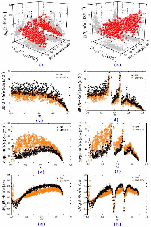
Refer to caption
Figure 4: The effects of RPV coupling Ξ»1​i​3′​λ1​i​2β€²β£βˆ—subscriptsuperscriptπœ†β€²1𝑖3subscriptsuperscriptπœ†β€²1𝑖2\lambda^{\prime}_{1i3}\lambda^{\prime*}_{1i2} due to the squark exchange in Bβ†’K(βˆ—)​e+​eβˆ’β†’π΅superscript𝐾superscript𝑒superscript𝑒B\to K^{(*)}e^{+}e^{-} and Bsβ†’e+​eβˆ’β†’subscript𝐡𝑠superscript𝑒superscript𝑒B_{s}\to e^{+}e^{-} decays. The primed observables are given with Οˆβ€‹(n​S)πœ“π‘›π‘†\psi(nS) VMD contributions, and Ο–italic-Ο–\varpi denote s^^𝑠\hat{s}.
Refer to caption
Figure 5: The effects of RPV coupling Ξ»i​11​λi​32β€²β£βˆ—subscriptπœ†π‘–11subscriptsuperscriptπœ†β€²π‘–32\lambda_{i11}\lambda^{\prime*}_{i32} due to the sneutrino exchange in Bβ†’K(βˆ—)​e+​eβˆ’β†’π΅superscript𝐾superscript𝑒superscript𝑒B\to K^{(*)}e^{+}e^{-} and Bsβ†’e+​eβˆ’β†’subscript𝐡𝑠superscript𝑒superscript𝑒B_{s}\to e^{+}e^{-} decays.
Refer to caption
Figure 6: The effects of RPV coupling Ξ»i​11βˆ—β€‹Ξ»i​23β€²subscriptsuperscriptπœ†π‘–11subscriptsuperscriptπœ†β€²π‘–23\lambda^{*}_{i11}\lambda^{\prime}_{i23} due to the sneutrino exchange in Bβ†’K(βˆ—)​e+​eβˆ’β†’π΅superscript𝐾superscript𝑒superscript𝑒B\to K^{(*)}e^{+}e^{-} and Bsβ†’e+​eβˆ’β†’subscript𝐡𝑠superscript𝑒superscript𝑒B_{s}\to e^{+}e^{-} decays.
Refer to caption
Figure 7: The effects of RPV coupling Ξ»2​i​3′​λ2​i​2β€²β£βˆ—subscriptsuperscriptπœ†β€²2𝑖3subscriptsuperscriptπœ†β€²2𝑖2\lambda^{\prime}_{2i3}\lambda^{\prime*}_{2i2} due to the squark exchange in Bβ†’K(βˆ—)​μ+β€‹ΞΌβˆ’β†’π΅superscript𝐾superscriptπœ‡superscriptπœ‡B\to K^{(*)}\mu^{+}\mu^{-} and Bsβ†’ΞΌ+β€‹ΞΌβˆ’β†’subscript𝐡𝑠superscriptπœ‡superscriptπœ‡B_{s}\to\mu^{+}\mu^{-} decays.
Refer to caption
Figure 8: The effects of RPV coupling Ξ»i​22​λi​32β€²β£βˆ—subscriptπœ†π‘–22subscriptsuperscriptπœ†β€²π‘–32\lambda_{i22}\lambda^{\prime*}_{i32} due to the sneutrino exchange in Bβ†’K(βˆ—)​μ+β€‹ΞΌβˆ’β†’π΅superscript𝐾superscriptπœ‡superscriptπœ‡B\to K^{(*)}\mu^{+}\mu^{-} and Bsβ†’ΞΌ+β€‹ΞΌβˆ’β†’subscript𝐡𝑠superscriptπœ‡superscriptπœ‡B_{s}\to\mu^{+}\mu^{-} decays.
Refer to caption
Figure 9: The effects of RPV coupling Ξ»i​22βˆ—β€‹Ξ»i​23β€²subscriptsuperscriptπœ†π‘–22subscriptsuperscriptπœ†β€²π‘–23\lambda^{*}_{i22}\lambda^{\prime}_{i23} due to the sneutrino exchange in Bβ†’K(βˆ—)​μ+β€‹ΞΌβˆ’β†’π΅superscript𝐾superscriptπœ‡superscriptπœ‡B\to K^{(*)}\mu^{+}\mu^{-} and Bsβ†’ΞΌ+β€‹ΞΌβˆ’β†’subscript𝐡𝑠superscriptπœ‡superscriptπœ‡B_{s}\to\mu^{+}\mu^{-} decays.