Abstract

Top-quark physics plays an important rôle at hadron colliders such as the Tevatron collider at Fermilab or the upcoming Large Hadron Collider (LHC) at CERN. Given the planned experimental precision, detailed theoretical predictions are mandatory. In this article we present analytic results for the complete electroweak corrections to gluon induced top-quark pair production, completing our earlier results for the quark-induced reaction. As an application we discuss top-quark pair production at Tevatron and at LHC. In particular we show that, although small for inclusive quantities, weak corrections can be sizeable for differential distribution.

I Introduction

Top-quark physics plays an important rôle at the Tevatron and will be an equally important topic at the upcoming LHC. In view of the large production rate, amounting to $\mathcal{O}(10^{8})$ top-quark pairs for an integrated luminosity of 200 ${\rm fb}^{-1}$, precise and direct measurements will be possible, which require a similarly detailed theoretical understanding of these reactions. Both single top-quark production as well as top-quark pair production have been studied extensively in the past. The differential cross section for top-quark pair production is known to next-to-leading order (NLO) accuracy in quantum chromodynamics (QCD) [1, 2, 3, 4, 5]. In addition, the resummation of logarithmic enhanced contributions has been studied in detail in Refs. [6, 7, 8, 9, 10, 11]. Recently also the spin correlations between top-quark and antitop-quark were calculated at NLO accuracy in QCD [5, 12].

Although formally suppressed through the small coupling, weak corrections can also be significant due to the presence of large Sudakov logarithms (see e.g. Refs. [13, 14] and references therein), which were also studied in the context of $\gamma$- and $Z$-production at hadron colliders [15, 16, 17]. The origin of these large logarithms is easily understood: at high scale the massive gauge bosons $W$ and $Z$ behave essentially like massless bosons. Collinear and soft phenomena thus lead to large negative corrections. In strictly massless theories like QED or QCD these contributions are cancelled through similar positive terms from the real corrections. This cancellation does not take place in the case of weak interaction because the real and virtual emission leads to different experimental signatures. Given that top-quark pair production at high scale is an ideal tool to search for new physics it is clear that the precise knowledge of the weak corrections in this region is of paramount importance. In Ref. [18] electroweak corrections to top-quark pair production in hadronic collisions were investigated for the first time. More precisely, the partonic sub-processes $q\bar{q}\to t\bar{t}$ and $gg\to t\bar{t}$ were studied. In a subsequent study [19] parity violating asymmetries were analysed in a two Higgs doublet model and the minimal supersymmetric standard model.

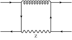
a)

$\raisebox{-28.45274pt}{\includegraphics[width=113.81102pt]{exgluonini}}\,\times\,\left(\,\,\raisebox{-28.45274pt}{\includegraphics[width=156.49014pt]{Zexgluonfin}}\right)^{\mbox{\Large$\ast$}}$

b)

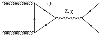
c)

Figure I.1: Pictorial representation of contributions missing in Ref. [18]

In the original works some contributions were omitted. For the quark–antiquark initiated process the gluon-$Z$ box contributions (Fig. I.1 a) and the corresponding real corrections (Fig. I.1 b) are missing in Ref. [18]. They were recently evaluated in Refs. [20, 21]. For the gluon fusion process a class of contributions related to triangle diagrams (Fig. I.1 c) are missing in Ref. [18], as noted also in Ref. [22], where the calculation of Ref. [18] has been repeated for the gluon induced top-quark pair production. In Ref. [22] no analytic results are presented. In view of the importance of the analysis for upcoming experiments it is the purpose of this paper to repeat the original calculation [18] — including all missing contributions — and present compact analytic results well suited for the experimental analysis.

The outline of the paper is as follows: In section II we present the calculation of the virtual electroweak corrections to top-quark pair production through gluon fusion. In contrast to the contributions from quark–antiquark annihilation there are no real corrections contributing to the weak corrections. The virtual corrections are thus infrared finite and represent the complete weak corrections for this channel. Compact analytic expressions in terms of scalar one-loop integrals are given in section II and in the appendix. In section III we present numerical results for the gluon fusion process at the parton level. Furthermore we combine the gluon channel with the quark–antiquark annihilation process (with the elctroweak corrections taken from Ref. [20]), fold them with parton distributions and give results for the corrections to the total cross section and to ${p_{T}}$- and ${\rm M}_{t\bar{t}}$- distributions relevant for the Tevatron and the LHC.

II Electroweak corrections to gluon fusion

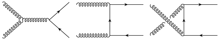
Figure II.1: Born diagrams for top-quark pair production via gluon fusion.

To setup our notation we start with the QCD tree-level contribution. The three contributions to the amplitude are shown in Fig. II.1. Evaluating the Feynman diagrams we obtain the well-known leading order differential cross section:

$${d\sigma_{\rm LO}\over dz}=\sigma_{0}\*{N^{2}\*(1+\beta^{2}\*z^{2})-2\over N\*(1-\beta^{2}\*z^{2})^{2}}\*\Big{(}1-\beta^{4}\*z^{4}+2\*\beta^{2}\*(1-\beta^{2})\*(1-z^{2})\Big{)}.$$ (II.1)

where $N$ is the number of colours, ${\alpha_{s}}$ the strong coupling constant and $\beta$ the velocity of the top-quark in the partonic centre-of-mass system:

$$\beta=\sqrt{1-{4{m_{t}}^{2}\over s}}$$ (II.2)

($s$ denotes the partonic centre-of-mass energy squared). The cosine of the scattering angle is denoted by $z$. Here and in what follows it is convenient to use the abbreviation

$$\sigma_{0}={\pi\alpha_{s}^{2}\over 4}{1\over N^{2}-1}{\beta\over s}.$$ (II.3)

A factor $1/(4\*(N^{2}-1)^{2})$ from averaging over the incoming spins and colour is included in the result above.

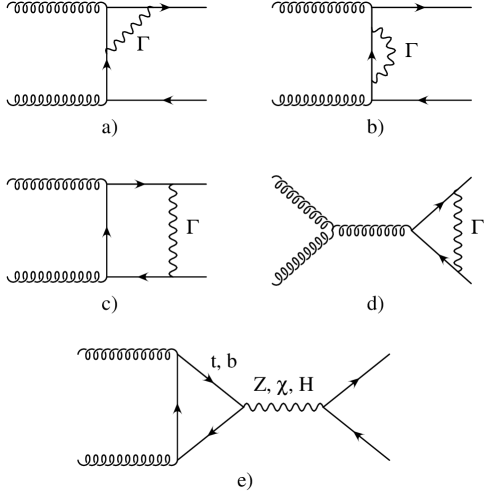
Figure II.2: Sample diagrams for the virtual corrections. $\Gamma$ stands for all contributions from gauge boson, goldstone boson and Higgs exchange.

For the calculation of the next-to-leading order weak corrections we use the ’t Hooft-Feynman gauge ($R_{\xi}$-gauge) with the gauge parameters $\xi^{i}$ set to 1. The longitudinal degrees of freedom of the massive gauge bosons $Z$ and $W$ are thus represented by the goldstone fields $\chi$ and $\phi$. Ghost fields do not contribute at the order under consideration. Sample diagrams are shown in Fig. II.2. The Cabibbo–Kobayashi–Maskawa mixing matrix is set to 1.
Before presenting the results for the weak corrections, let us add a few technical remarks. We use the Passarino –Veltman reduction scheme [23] to reduce analytically the tensor integrals to scalar integrals. For these the following convention is used:

$$X_{0}={1\over i\pi^{2}}\int d^{d}\ell{(2\pi\mu)^{2\varepsilon}\over(\ell^{2}-m_{1}^{2}+i\epsilon)\cdots}.$$ (II.4)

For the UV-divergent integrals we define the finite part for the one-point integrals $A_{0}$ and the two-point integrals $B_{0}$ through

$$A_{0}(m^{2}) = m^{2}\Delta+\overline{A}_{0}(m^{2}),$$

$$B_{0}(p^{2},m_{1}^{2},m_{2}^{2}) = \Delta+\overline{B}_{0}(p^{2},m_{1}^{2},m_{2}^{2}),$$ (II.5)

with $\Delta=1/\varepsilon-\gamma+\ln(4\pi)$. The renormalisation is performed in the counterterm formalism, where the bare Lagrangian $\cal L$ is rewritten in terms of renormalised fields and couplings:

$${\cal L}(\Psi_{0},A_{0},m_{0},g_{0}) = {\cal L}(Z^{1/2}_{\Psi}\Psi_{R},Z^{1/2}_{A}A_{R},Z_{m}m_{R},Z_{g}g_{R})$$ (II.6)

$$\equiv {\cal L}(\Psi_{R},A_{R},m_{R},g_{R})+{\cal L}_{ct}(\Psi_{R},A_{R},m_{R},g_{R}).$$

The contribution ${\cal L}(\Psi_{R},A_{R},m_{R},g_{R})$ gives just the ordinary Feynman rules, but with the bare couplings replaced by the renormalised ones. The complete list of Feynman rules can be found for example in Ref. [24]. The contribution ${\cal L}_{ct}(\Psi_{R},A_{R},m_{R},g_{R})$ in Eq. (II.6) yields the counterterms, which render the calculation ultraviolet (UV)-finite. Some of the resulting diagrams are shown in Fig. II.3.

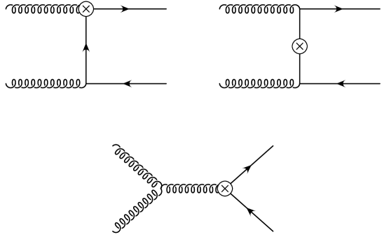
Figure II.3: Sample counterterm diagrams.

For the present calculation only wave function and mass renormalisation are needed. No coupling constant renormalisation has to be performed. This is a consequence of the fact, that although the weak corrections appear as a loop-correction, they are still leading-order in the electroweak couplings. Mass and wave function renormalisation are performed in the on-shell scheme:

$$m_{t,0} = m_{t}+\delta m_{t},$$ (II.7)

$$\Psi^{R,L}_{t,0} = \left(Z_{t}^{R,L}\right)^{1/2}\Psi^{R,L}_{t}=\left(1+{1\over 2}\delta Z_{t}^{R,L}\right)\Psi^{R,L}_{t}.$$ (II.8)

The renormalisation constants are thus given in terms of self-energy corrections $\Sigma$ and their derivatives:

$$\delta Z_{\rm V} = {1\over 2}(\delta Z_{t}^{L}+\delta Z_{t}^{R})=-\Sigma_{\rm V}(p^{2}={m_{t}}^{2})-2\*{m_{t}}^{2}{\partial\over\partial p^{2}}\left(\Sigma_{\rm V}+\Sigma_{\rm S}\right)\Big{|}_{p^{2}={m_{t}}^{2}}\;,$$

$$\delta Z_{\rm A} = {1\over 2}(\delta Z_{t}^{L}-\delta Z_{t}^{R})=-\Sigma_{\rm A}(p^{2}={m_{t}}^{2}),$$

$${\delta{m_{t}}\over{m_{t}}} = -\Sigma_{\rm V}(p^{2}={m_{t}}^{2})-\Sigma_{\rm S}(p^{2}={m_{t}}^{2}).$$ (II.9)

The functions $\Sigma_{\rm V,A,S}$ can be found for example in Ref. [24]. Here we need only $\delta Z_{\rm V}$ and ${\delta{m_{t}}/{m_{t}}}$. Their explicit form in terms of scalar integrals — using the notation of this paper — reads:

$$\delta Z_{\rm V} = {\alpha\over 4\*\pi}\*\Bigg{\{}\Big{[}{g_{v}^{t}}^{2}+{g_{a}^{t}}^{2}+{1\over{m_{t}}^{2}}\*({g_{v}^{t}}^{2}+{g_{a}^{t}}^{2})\*\Big{(}{{A}_{0}({m_{Z}}^{2})}-{{A}_{0}({m_{t}}^{2})}-{m_{Z}}^{2}\*{{B}_{0}^{Z}}\Big{)}$$ (II.10)

$$+ \Big{(}2\*({g_{v}^{t}}^{2}+{g_{a}^{t}}^{2})\*{m_{Z}}^{2}+4\*{m_{t}}^{2}\*({g_{v}^{t}}^{2}-3\*{g_{a}^{t}}^{2})\Big{)}\*{{d\over dp^{2}}B_{0}^{Z}\Big{|}_{p^{2}=mt^{2}}}\Big{]}$$

$$+ \*{1\over 2\*s_{W}^{2}}\*\Big{[}{1\over 2}+{1\over 2\*{m_{t}}^{2}}\*\Big{(}{{A}_{0}({m_{W}}^{2})}-{{A}_{0}({m_{b}}^{2})}\Big{)}-{{m_{t}}^{2}-{m_{b}}^{2}+{m_{W}}^{2}\over 2\*{m_{t}}^{2}}\*{{B}_{0}^{W}}$$

$$- ({m_{t}}^{2}-{m_{W}}^{2}+{m_{b}}^{2})\*{{d\over dp^{2}}B_{0}^{W}\Big{|}_{p^{2}=mt^{2}}}\Big{]}$$

$$+ \*{{m_{t}}^{2}\over 4\*s_{W}^{2}\*{m_{W}}^{2}}\*\Big{[}{1\over 2\*{m_{t}}^{2}}\*\Big{(}{{A}_{0}({m_{Z}}^{2})}-{{A}_{0}({m_{t}}^{2})}-{m_{Z}}^{2}\*{{B}_{0}^{Z}}\Big{)}$$

$$+ {m_{Z}}^{2}\*{{d\over dp^{2}}B_{0}^{Z}\Big{|}_{p^{2}=mt^{2}}}\Big{]}$$

$$+ \*{1\over 2\*s_{W}^{2}}\*{1\over 4\*{m_{W}}^{2}}\*\Big{[}{{m_{t}}^{2}+{m_{b}}^{2}\over{m_{t}}^{2}}\*\Big{(}{{A}_{0}({m_{W}}^{2})}-{{A}_{0}({m_{b}}^{2})}\Big{)}$$

$$- {({m_{t}}^{2}-{m_{b}}^{2}+{m_{W}}^{2})\*({m_{t}}^{2}+{m_{b}}^{2})\over{m_{t}}^{2}}\*{{B}_{0}^{W}}$$

$$- 2\*\Big{(}({m_{t}}^{2}-{m_{b}}^{2})^{2}-{m_{W}}^{2}\*({m_{t}}^{2}+{m_{b}}^{2})\Big{)}\*{{d\over dp^{2}}B_{0}^{W}\Big{|}_{p^{2}=mt^{2}}}\Big{]}$$

$$+ \*{{m_{t}}^{2}\over 4\*s_{W}^{2}\*{m_{W}}^{2}}\*\Big{[}{1\over 2\*{m_{t}}^{2}}\*\Big{(}{{A}_{0}({m_{H}}^{2})}-{{A}_{0}({m_{t}}^{2})}-{m_{H}}^{2}\*{{B}_{0}^{H}}\Big{)}$$

$$- (4\*{m_{t}}^{2}-{m_{H}}^{2})\*{{d\over dp^{2}}B_{0}^{H}\Big{|}_{p^{2}=mt^{2}}}\Big{]}\Bigg{\}},$$

$${\delta{m_{t}}\over{m_{t}}} = -{\alpha\over 4\*\pi}\*\Bigg{\{}{1\over{m_{t}}^{2}}\Big{[}(3\*{g_{a}^{t}}^{2}-{g_{v}^{t}}^{2})\*{m_{t}}^{2}+({g_{v}^{t}}^{2}+{g_{a}^{t}}^{2})\Big{(}{{A}_{0}({m_{t}}^{2})}-{{A}_{0}({m_{Z}}^{2})}\Big{)}$$ (II.11)

$$+ \Big{(}({g_{v}^{t}}^{2}+{g_{a}^{t}}^{2})\*{m_{Z}}^{2}+2\*{m_{t}}^{2}\*({g_{v}^{t}}^{2}-3\*{g_{a}^{t}}^{2})\Big{)}\*{{B}_{0}^{Z}}\Big{]}$$

$$+ {1\over 4\*s_{W}^{2}\*{m_{t}}^{2}}\*\Big{[}{m_{t}}^{2}+\*\Big{(}{{A}_{0}({m_{b}}^{2})}-{{A}_{0}({m_{W}}^{2})}\Big{)}+({m_{W}}^{2}-{m_{b}}^{2}-{m_{t}}^{2})\*{{B}_{0}^{W}}\Big{]}$$

$$+ {1\over 8\*s_{W}^{2}\*{m_{W}}^{2}}\*\Big{[}{{A}_{0}({m_{t}}^{2})}-{{A}_{0}({m_{Z}}^{2})}+{m_{Z}}^{2}{{B}_{0}^{Z}}\Big{]}$$

$$+ {1\over 8\*s_{W}^{2}\*{m_{W}}^{2}\*{m_{t}}^{2}}\*\Big{[}({m_{t}}^{2}+{m_{b}}^{2})\*\Big{(}{{A}_{0}({m_{b}}^{2})}-{{A}_{0}({m_{W}}^{2})}\Big{)}$$

$$- \Big{(}({m_{t}}^{2}-{m_{b}}^{2})^{2}-{m_{W}}^{2}\*({m_{t}}^{2}+{m_{b}}^{2})\Big{)}\*{{B}_{0}^{W}}\Big{]}$$

$$+ {1\over 8\*s_{W}^{2}\*{m_{W}}^{2}}\*\Big{[}{{A}_{0}({m_{t}}^{2})}-{{A}_{0}({m_{H}}^{2})}+({m_{H}}^{2}-4\*{m_{t}}^{2})\*{{B}_{0}^{H}}\Big{]}\Bigg{\}},$$

where ${s_{W}}$ (${c_{W}}$) denotes the sine (cosine) of the weak mixing angle. The vector $({g_{v}^{t}})$ and axial-vector $({g_{a}^{t}})$ couplings of the top-quark to the $Z$-boson are given in terms of the weak isospin $T_{3}^{f}$ and the electric charge $Q_{f}$ for a fermion of flavour $f$:

$${g_{v}^{f}} = {1\over 2{s_{W}}{c_{W}}}(T_{3}^{f}-2{s_{W}}^{2}Q_{f}),$$ (II.12)

$${g_{a}^{f}} = {1\over 2{s_{W}}{c_{W}}}T_{3}^{f}.$$ (II.13)

The coupling of the top-quark to the $W$-boson is given by

$${g_{W}}={1\over 2\sqrt{2}{s_{W}}}.$$ (II.14)

As usual $\alpha$ stands for the fine structure constant, which will be taken as running coupling evaluated at the scale $2{m_{t}}$. The mass of particle $i$ is denoted by $m_{i}$. The abbreviations $B_{0}^{Z,W,H}$ for the two-point scalar loop-integrals are defined in the appendix. Note that the photonic corrections form a gauge independent subset and are not included in Eqs. II.10, II.11 and in the following discussion.

For the following discussion it is convenient to separate the weak corrections into the contribution from vertex-diagrams ($t$-, $u$-channel, $s$-channel, Fig. II.2 a,d), self-energy-diagrams (Fig. II.2 b) and box-diagrams (Fig. II.2 c). The triangle diagrams in (Fig. II.2 e) are finite without renormalisation and will be studied separately. The differential cross section at next-to-leading order is decomposed as follows:

$${d\sigma^{\rm NLO}\over dz}=\sum_{i=Z,W,\chi,\phi,H}{d\sigma_{i}^{\Box}\over dz}+{d\sigma_{i}^{V}\over dz}+{d\sigma_{i}^{sV}\over dz}+{d\sigma_{i}^{{\Sigma}}\over dz}+\sum_{i=Z,\chi,H}{d\sigma_{i}^{{\bigtriangleup}}\over dz}.$$ (II.15)

We start with the analytic results for the triangle diagrams. For the Higgs and $(Z+\chi)$-terms we obtain

$${d\sigma^{\bigtriangleup}_{H}\over dz} = {\alpha\*\over\pi}\*\sigma_{0}\*{{m_{t}}^{2}\over{m_{W}}^{2}\*s_{W}^{2}}\*{\beta^{2}\over 1-\beta^{2}\*z^{2}}\*{1\over s-{m_{H}}^{2}}$$

$$\*\Big{[}{m_{t}}^{2}\*(s-4\*{m_{t}}^{2})\*C_{0}^{t}+{m_{b}}^{2}\*(s-4\*{m_{b}}^{2})\*C_{0}^{b}-2\*({m_{t}}^{2}+{m_{b}}^{2})\Big{]},$$

$${d\sigma^{\bigtriangleup}_{Z+\chi}\over dz}=16\*{\alpha\over\pi}\*\sigma_{0}\*{{g_{a}^{t}}}\*{{m_{t}}^{2}\over{m_{Z}}^{2}\*(1-\beta^{2}\*z^{2})}\*\Big{(}{g_{a}^{t}}\*{m_{t}}^{2}\*C_{0}^{t}+g_{a}^{b}\*{m_{b}}^{2}\*C_{0}^{b}\Big{)},$$ (II.17)

A factor $1/(4\*(N^{2}-1)^{2})$ from averaging over the incoming spins and colour is again included. The integrals $C_{0}^{b,t}$ are defined in the appendix. As a consequence of Furry’s theorem only the axial-vector induced terms contribute in the case where the $Z$-boson appears in the $s$-channel. Furthermore, the Landau–Yang theorem forbids the decay of an on-shell vector boson into two identical massless on-shell spin-one bosons. Therefore, the poles from the propagators of the $Z$-boson and the $\chi$ are cancelled in the $\sigma^{\bigtriangleup}_{Z+\chi}$-term, as evident from Eq. (II.17).

For the remaining vertex corrections with a gluon in the $s$-channel we obtain

$${d\sigma^{sV}_{Z}\over dz} = -2\*{\alpha\over\pi}\*\sigma_{0}\*N\*{{m_{t}}^{2}\over s^{2}}\*{z^{2}\over 1-\beta^{2}\*z^{2}}\*\Bigg{\{}$$ (II.18)

$$2\*\Big{[}2\*({g_{v}^{t}}^{2}+{g_{a}^{t}}^{2})\*{m_{Z}}^{2}-s\*\beta^{2}\*({g_{v}^{t}}^{2}-3\*{g_{a}^{t}}^{2})\Big{]}\*\Big{(}{\overline{B}_{0}^{t}}-{\overline{B}_{0}^{Z}}\Big{)}$$

$$+ \Big{[}4\*({g_{v}^{t}}^{2}+{g_{a}^{t}}^{2})\*{m_{Z}}^{4}+8\*{g_{a}^{t}}^{2}\*{m_{Z}}^{2}\*s\*\beta^{2}$$

$$- s^{2}\*\beta^{2}\*({g_{v}^{t}}^{2}+{g_{a}^{t}}^{2}+\beta^{2}\*({g_{v}^{t}}^{2}-3\*{g_{a}^{t}}^{2}))\Big{]}\*C_{0}^{Z}$$

$$+ s\*\beta^{2}\*\Big{[}2\*{m_{Z}}^{2}\*({g_{v}^{t}}^{2}+{g_{a}^{t}}^{2})$$

$$+ s\*(1-\beta^{2})\*({g_{v}^{t}}^{2}-3\*{g_{a}^{t}}^{2})\Big{]}\*{{d\over dp^{2}}B_{0}^{Z}\Big{|}_{p^{2}=mt^{2}}}\Bigg{\}},$$

$${d\sigma^{sV}_{W}\over dz} = -8\*{\alpha\over\pi}\*\sigma_{0}\*{g_{W}}^{2}\*N\*{{m_{t}}^{2}\over s^{2}}\*{z^{2}\over 1-\beta^{2}\*z^{2}}\*\Bigg{\{}$$ (II.19)

$${1\over 2}\*(s\*(1+\beta^{2})+4\*({m_{W}}^{2}-{m_{b}}^{2}))\*\Big{(}{\overline{B}_{0}^{b}}-{\overline{B}_{0}^{W}}\Big{)}$$

$$+ {1\over 8}\*\Big{(}\big{(}s\*(1+\beta^{2})+4\*({m_{W}}^{2}-{m_{b}}^{2})\big{)}^{2}-4\*\beta^{2}\*s^{2}\Big{)}\*C_{0}^{W}$$

$$- {1\over 4}\*s\*\beta^{2}\*\Big{(}s\*(1-\beta^{2})+4\*({m_{b}}^{2}-{m_{W}}^{2})\Big{)}\*{{d\over dp^{2}}B_{0}^{W}\Big{|}_{p^{2}=mt^{2}}}\Bigg{\}},$$

$${d\sigma^{sV}_{\chi}\over dz} = -8\*{\alpha\over\pi}\*{\sigma_{0}}\*{g_{a}^{t}}^{2}\*N\*{{m_{t}}^{4}\over s^{2}}\*{z^{2}\over 1-\beta^{2}\*z^{2}}\*\Bigg{\{}2\*\Big{(}{\overline{B}_{0}^{t}}-{\overline{B}_{0}^{Z}}\Big{)}$$ (II.20)

$$+ (2\*{m_{Z}}^{2}+s\*\beta^{2})\*C_{0}^{Z}+s\*\beta^{2}\*{{d\over dp^{2}}B_{0}^{Z}\Big{|}_{p^{2}=mt^{2}}}\Bigg{\}},$$

$${d\sigma^{sV}_{\phi}\over dz} = -8\*{\alpha\over\pi}\*\sigma_{0}\*{{g_{W}}^{2}\over{m_{W}}^{2}}\*N\*{{m_{t}}^{2}\over s^{2}}\*{z^{2}\over 1-\beta^{2}\*z^{2}}\*\Bigg{\{}{1\over 16}\*\Big{(}16\*{m_{b}}^{4}+{m_{b}}^{2}\*(8\*s\*\beta^{2}-16\*{m_{W}}^{2})$$ (II.21)

$$- 4\*{m_{W}}^{2}\*s\*(1-\beta^{2})-s^{2}\*(1-\beta^{4})\Big{)}\*\Big{(}{\overline{B}_{0}^{W}}-{\overline{B}_{0}^{b}}\Big{)}$$

$$+ {1\over 64}\*\Big{[}64\*{m_{b}}^{6}-16\*{m_{b}}^{4}\*(8\*{m_{W}}^{2}+s\*(1-\beta^{2}))$$

$$+ 16\*{m_{W}}^{4}\*s\*(1-\beta^{2})+4\*{m_{b}}^{2}\*(16\*{m_{W}}^{4}-s^{2}\*(1-\beta^{2})^{2})$$

$$+ 8\*{m_{W}}^{2}\*s^{2}\*(1-\beta^{4})+s^{3}\*(1-\beta^{2})^{3}\Big{]}\*C_{0}^{W}$$

$$- {1\over 32}\*\Big{[}16\*{m_{b}}^{4}\*s\*\beta^{2}-8\*{m_{b}}^{2}\*(2\*{m_{W}}^{2}\*s\*\beta^{2}+s^{2}\*\beta^{2}\*(1-\beta^{2}))$$

$$- 4\*{m_{W}}^{2}\*s^{2}\*\beta^{2}\*(1-\beta^{2})+s^{3}\*\beta^{2}\*(1-\beta^{2})^{2}\Big{]}\*{{d\over dp^{2}}B_{0}^{W}\Big{|}_{p^{2}=mt^{2}}}\Bigg{\}},$$

$${d\sigma^{sV}_{H}\over dz} = 4\*{\alpha\over\pi}\*\sigma_{0}\*{g_{W}}^{2}\*N\*{{m_{t}}^{2}\over s^{2}}\*{z^{2}\over 1-\beta^{2}\*z^{2}}\*{{m_{t}}^{2}\over{m_{W}}^{2}}\*\Bigg{\{}$$ (II.22)

$$2\*(s\*\beta^{2}+{m_{H}}^{2})\*\Big{(}{\overline{B}_{0}^{H}}-{\overline{B}_{0}^{t}}\Big{)}$$

$$+ \Big{(}s^{2}\*\beta^{2}\*(1-\beta^{2})-3\*{m_{H}}^{2}\*s\*\beta^{2}-2\*{m_{H}}^{4}\Big{)}\*C_{0}^{H}$$

$$+ s\*\beta^{2}\*(s\*(1-\beta^{2})-{m_{H}}^{2})\*{{d\over dp^{2}}B_{0}^{H}\Big{|}_{p^{2}=mt^{2}}}\Bigg{\}}.$$

The remaining contributions to the differential cross section are listed in appendix B.

Before showing concrete results for hadron colliders we first discuss several checks of our result. We performed two independent calculations yielding also two independent numerical computer codes. We checked that we obtain the correct structure for the UV singularities yielding a finite result after renormalisation. In our notation this corresponds to a stringent test of the coefficients of the $A_{0}$- and $B_{0}$-integrals. The behaviour of the Higgs corrections close to threshold and for light Higgs bosons is well understood (see for example Ref. [25] and references therein). This allows to test the Higgs contributions for a very light Higgs near threshold. For a $t\bar{t}$-system produced through a vector current the Higgs correction is given by the factor $(1+H_{\rm thr}(r))$ with

$$H_{{\rm thr}}(r) = {2\*\kappa\over\pi}\*\Bigg{\{}-{1\over 12}\*\Bigg{[}-12+4\*r+(-12+9\*r-2\*r^{2})\ln\left(r\right)$$ (II.23)

$$+ {2\over r}\*(-6+5\*r-2\*r^{2})\*\sqrt{r\*(4-r)}\*\arccos\left({\sqrt{r}\over 2}\right)\Bigg{]}$$

$$- {\pi\over\sqrt{r}}+{\pi\over 2\*\beta}\*\arctan\left({2\*\beta\over\sqrt{r}}\right)\Bigg{\}}$$

and

$$r={{m_{H}}^{2}\over{m_{t}}^{2}},\quad\kappa={\alpha\over 4}\*{{m_{t}}^{2}\over{s_{W}}^{2}\*{m_{W}}^{2}}.$$ (II.24)

Figure II.4: Comparison of the full corrections from Higgs boson exchange with the corrections based on Eq. (II.23) (${m_{H}}=0.1\mbox{ MeV}$).

In Fig. II.4 we show the numerical result for ${m_{H}}=0.1\mbox{ MeV}$ as function of the variable $\eta$ defined through

$$\eta={s\over 4{m_{t}}^{2}}-1.$$ (II.25)

The line shows the Higgs contribution according to Eq. (II.23). The crosses show the result from the full Higgs boson induced correction. The enhancement proportional to $1/\beta$ is well recovered by the calculation. The numerical agreement is between four ($\eta=10^{-5}$) and two digits ($\eta=10^{-3}$). As we shall see later the enhancement close to threshold for a light Higgs can still be observed even for a Higgs mass of 120 GeV although reduced to 2%. A similar test has been performed for a light $Z$-boson. Again we find perfect agreement. In addition we compared analytically the results for the $t$- and $u$-channel vertices, self-energies and Higgs triangle diagrams with those from Ref. [18]. We find complete agreement, after the correction of some typos in Ref. [18]. Using the same input parameters we also compared the plots shown in Ref. [18] and found agreement. Finally we compared numerically with the results of Ref. [26] and found perfect agreement. However, we are in disagreement with the results published recently in Ref. [22]. In particular for the ${p_{T}}$ and ${\rm M}_{t\bar{t}}$ distribution we find negative corrections close to threshold while the corrections are positive in Ref. [22] (Fig. 1). Our findings are also confirmed in Ref. [26].

III Numerical results

Figure III.1: Different contributions to the electroweak corrections: Vertices (long-dashed), self-energies (dashed), boxes (dotted), triangles (dash-dotted). The sum is shown as full line.

In this section we present numerical results for the gluon fusion process at order $\alpha_{s}^{2}\alpha$. We use the following coupling constants:

$$\alpha(2{m_{t}})={1\over 126.3},\quad{\alpha_{s}}=0.1,\quad{s_{W}}^{2}=0.231,$$

and, if not stated otherwise, the following masses:

$${m_{Z}}=91.1876\mbox{ GeV},\quad{m_{W}}=80.425\mbox{ GeV},\quad{m_{H}}=120\mbox{ GeV},\,$$

$${m_{b}}=4.82\mbox{ GeV},\quad{m_{t}}=172.7\mbox{ GeV}.$$

The parameters ${s_{W}}$, ${m_{Z}}$ and ${m_{W}}$ are, of course, interdependent. Nevertheless, we expect that, using the ${\overline{\mbox{MS}}}$ value for the weak mixing angle, some of (uncalculated) higher-order corrections are included and, therefore, a better phenomenological description is achieved. The difference between using the ${\overline{\mbox{MS}}}$ and the on-shell input respectively, is formally of higher-order.

In Fig. III.1 the separate corrections as defined in Eq. (II.15) are shown at the parton level. We normalise the result to the leading-order $gg\to t\bar{t}$ process. The sum of the different contributions is shown as a solid line in Fig. III.1. For moderate partonic energies the corrections are of the order of a few percent as one might have expected for a weak correction. Near threshold the cross section is dominated by the triangle- and the box-diagrams. Both are of the same order of magnitude, but opposite in sign, leading to a significant cancellation. It is worth noting at this point that the inclusion of the ($Z+\chi$)-triangle diagrams — neglected in Ref. [18] — decreases the result by about 2% in the threshold region (${m_{H}}=$ 120 GeV). The ($Z+\chi$)-term dominates the triangle contributions. In Fig. III.2 we illustrate the effect of $\sigma^{\bigtriangleup}_{Z+\chi}$ by comparing the full result with the result where $\sigma^{\bigtriangleup}_{Z+\chi}$ is neglected. Close to the threshold the aforementioned 2% difference is observed. The ($Z+\chi$)-contribution accidentally compensates the positive contribution from Higgs exchange, which however, becomes small about 20 GeV above threshold. For energies above 600 GeV the contribution from the ($Z+\chi$)-triangle becomes negligible. The behaviour of the box contribution close to the threshold, shown in Fig. III.1, is a consequence of the Higgs effects discussed before.

Figure III.2: Comparison between the electroweak corrections: with the $Z$ and $\chi$ triangle diagrams included (full) and without these contributions (dashed).

On the other hand for a partonic centre-of-mass energy of around 500 GeV the large negative Sudakov logarithms start to become important and amount to more than 10 percent at a few TeV. If we compare the relative size of the weak correction for gluon and quark–antiquark induced reactions at large energies, we find that they are twice as large for the quark–antiquark process. This can be qualitatively understood by just counting the external lines which can emit $W$- and $Z$-bosons, and observing that the corrections start to be dominated by Sudakov logarithms.

Figure III.3: The dependence of the partonic cross section from the Higgs mass: ${m_{H}}=120\mbox{ GeV}$ (full line), ${m_{H}}=180\mbox{ GeV}$ (dashed), ${m_{H}}=240\mbox{ GeV}$ (dashed-dotted) and ${m_{H}}=1000\mbox{ GeV}$ (dotted).

The dependence on the Higgs mass, i.e. the relative corrections for different Higgs masses are shown in Fig. III.3. For Higgs masses larger than $2{m_{t}}$ we include the width of the Higgs boson in the $s$-channel propagator.

$${1\over s-{m_{H}}^{2}}\rightarrow{1\over s-{m_{H}}^{2}+i{m_{H}}\Gamma_{H}}.$$ (III.1)

The corrections are strongly dependent on ${m_{H}}$ with a variation of nearly 6% in the threshold region.

Figure III.4: Electroweak corrections to top-quark pair production at the Tevatron (upper figure) and the LHC (lower figure) for three different Higgs masses (${m_{H}}=120\mbox{ GeV}$ (full line), ${m_{H}}=200\mbox{ GeV}$ (dashed), ${m_{H}}=1000\mbox{ GeV}$ (dashed-dotted)).

Let us now address the effects of the weak corrections on hadronic observables. We used the parton distribution function CTEQ6L [27] evaluated at a factorisation scale $\mu_{F}=2{m_{t}}$. With the input mentioned before we obtain

$$\sigma^{\rm TeV} = \sigma_{q\bar{q}}^{\rm TeV}+\sigma_{gg}^{\rm TeV}=4.18\,\,{\rm pb}+0.19\,\,{\rm pb}=4.37\,\,{\rm pb}$$

and

$$\sigma^{\rm LHC} = \sigma_{q\bar{q}}^{\rm LHC}+\sigma_{gg}^{\rm LHC}=56\,\,{\rm pb}+366\,\,{\rm pb}=422\,\,{\rm pb}$$

for the leading-order cross section at the Tevatron respectively LHC. The leading-order estimate is significantly smaller than the QCD corrected (NLO + resummation) result of about 6.7 pb for the Tevatron [11] and about 794 pb for the LHC [28]. To some extend the large QCD corrections are of universal character and it is plausible that lowest order and electroweak corrected (total and differential) cross sections will be affected by similar corrections. Therefore we will, in the following, only present their relative size. In a first step we study the weak corrections to the total cross section at the Tevatron and the LHC as a function of ${m_{t}}$ for three different Higgs masses ( Fig. III.4). The results include both quark–antiquark annihilation and gluon fusion. As expected the corrections to the inclusive cross section amount to a few percent only. Most of the top-quark pairs are produced close to threshold, where the weak corrections at parton level amount to a few percent only. The relative corrections are essentially given by the threshold behaviour of the quark–antiquark channel for the Tevatron and the gluon channel for the LHC. The integrated cross section samples a wide range in ${\rm M}_{t\bar{t}}$, and the marked Higgs mass dependence of the partonic cross section close to threshold is washed out. The correction is nearly independent of the top-quark mass for values of ${m_{t}}$ between 165 and 180 GeV. Given the experimental precision at the Tevatron and the LHC it is unlikely that the weak corrections can be seen in the total cross section. Differential distributions in ${p_{T}}$ and ${\rm M}_{t\bar{t}}$ are affected however, strongly. Indeed, the corrections to the ${\rm M}_{t\bar{t}}$-distributions can be directly read off from Fig. III.3, as far as the gluon induced channel is concerned. Note that for the quark–antiquark process the situation is more involved due to the presence of real corrections [20]. In principle it might be possible to establish the enhancement induced by the top-quark Yukawa coupling for a relatively light Higgs boson. However, the difference of 6% between a light ($120$ GeV) and a heavy ($1000$ GeV) Higgs boson could be masked by QCD uncertainties which are particularly large in the threshold region. In contrast, the weak corrections amount to more than ten percent at high energy when the Sudakov suppression becomes large. Therefore we study their effect on differential distributions at large momentum transfer. With the differential distribution in the top-antitop invariant mass (${\rm M}_{t\bar{t}}=\sqrt{(k_{t}+k_{\bar{t}})^{2}}$) being a sensitive tool in the search for new physics, this question is of particular importance. At large momentum transfer two competing effects must be considered: The logarithmically increasing Sudakov logarithms, and the increasing statistical uncertainty.

Figure III.5: Leading-order differential cross section for LHC as a function of ${p_{T}}$ and ${\rm M}_{t\bar{t}}$. Shown is the sum (full) and the contributions from gluon fusion (dashed) and quark–antiquark annihilation (dotted).

Figure III.6: Leading-order differential cross section for Tevatron as a function of ${p_{T}}$ and ${\rm M}_{t\bar{t}}$. Shown is the sum (full) and the contributions from gluon fusion (dashed) and quark–antiquark annihilation (dotted).

To get a rough idea about the possible statistical sensitivity we show in Fig. III.5 and Fig. III.6 the leading-order differential cross sections in ${\rm M}_{t\bar{t}}$ respectively ${p_{T}}$. For LHC, about $10^{8}$ events are expected for an integrated luminosity of $200\,\,{\rm fb^{-1}}$ and large values of ${\rm M}_{t\bar{t}}$ and ${p_{T}}$ will be accessible. An interesting behaviour of the relative importance of gluon- versus quark-induced processes is observed for the LHC. For low ${\rm M}_{t\bar{t}}$ and ${p_{T}}$ the gluon channel dominates. However for ${p_{T}}$ larger than 1 TeV the quark–antiquark annihilation process takes over, as a consequence of the change in relative importance of quark–antiquark versus gluon luminosities. For the Tevatron only moderate values of $300$ GeV for ${p_{T}}$ and $700$ GeV for ${\rm M}_{t\bar{t}}$ are accessible at best. Furthermore, the quark–antiquark annihilation process dominates through out.

Figure III.7: The relative corrections to the ${p_{T}}$- and ${\rm M}_{t\bar{t}}$- distribution for the LHC for ${m_{H}}=120$ GeV (bold line) and ${m_{H}}=1000$ GeV (thin line).

Figure III.8: The relative corrections to the ${p_{T}}$- and ${\rm M}_{t\bar{t}}$- distribution for the Tevatron for ${m_{H}}=120$ GeV (bold line) and ${m_{H}}=1000$ GeV (thin line).

The relative corrections of the differential distributions in ${p_{T}}$ and ${\rm M}_{t\bar{t}}$ are shown in Fig. III.7 and  III.8 for the LHC and Tevatron. For large values of ${p_{T}}$ and ${\rm M}_{t\bar{t}}$, accessible at the LHC, sizeable negative corrections are predicted, reaching ten up to fifteen percent. In contrast, the corrections are far smaller at the Tevatron. Taking ${m_{H}}=120\,\,{\rm GeV}$, they are $+3\%$ close to threshold and $-5\%$ for ${\rm M}_{t\bar{t}}$ around $800$ GeV, leading to a distortion of the differential distribution by $8\%$. It remains to be seen, whether QCD and experimental uncertainties can be pushed below this level. A rough guess of the statistical uncertainty expected for LHC and Tevatron can be deduced from Figs. III.9 and Fig. III.10. The estimated number of events with ${\rm M}_{t\bar{t}}\geq{\rm M}_{t\bar{t}}^{\rm cut}$, based on a luminosity of $200{\rm fb^{-1}}$ for the LHC ($8{\rm fb^{-1}}$ for the Tevatron) is used to estimate the statistical uncertainty and compared with the relative corrections, evaluated for the same sample. It will be difficult to observe the effect of the electroweak corrections at the Tevatron. At the LHC, with the large sample of top quarks, the statistical precision will match the size of the electroweak Sudakov logarithms, and eventually of the Higgs enhancement in the threshold region.

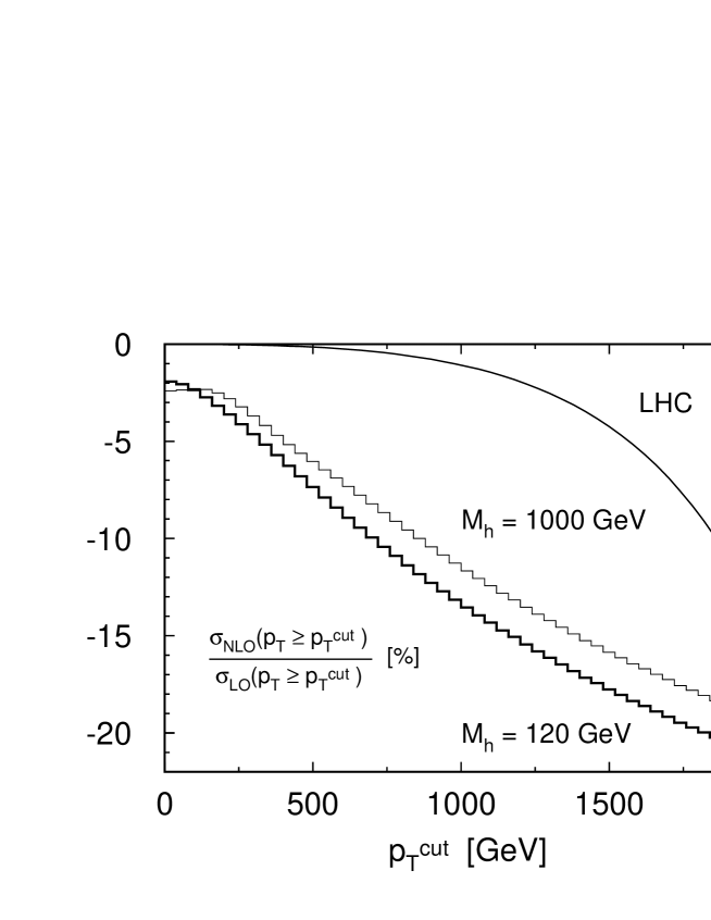
Figure III.9: The relative corrections to the ${p_{T}}$- and ${\rm M}_{t\bar{t}}$-distributions, integrated from a lower value in ${p_{T}}$ respectively ${\rm M}_{t\bar{t}}$ to the kinematic limit, for the LHC and two Higgs masses (${m_{H}}=120$ GeV (bold line), ${m_{H}}=1000$ GeV (thin line)). The smooth curve gives an estimate of the corresponding statistical uncertainty for an integrated luminosity of $200\,\,{\rm fb^{-1}}$.

Figure III.10: The relative corrections to the ${p_{T}}$- and ${\rm M}_{t\bar{t}}$-distributions, integrated from a lower value in ${p_{T}}$ respectively ${\rm M}_{t\bar{t}}$ to the kinematic limit, for the Tevatron and two Higgs masses (${m_{H}}=120$ GeV (bold line), ${m_{H}}=1000$ GeV (thin line)). The smooth curve gives an estimate of the corresponding statistical uncertainty for an integrated luminosity of $8\,\,{\rm fb^{-1}}$.

Before closing this discussion, let us mention that also the dependence of the corrections on the bottom-mass was investigated and the full dependence on the bottom quark mass was kept throughout. Furthermore the results can also be used to study weak corrections for $b$-quark pair production. This topic will be discussed in a subsequent publication. For a massless bottom-quark the $W$, $\phi$ contributions and the $Z$, $\chi$ triangles differ at most one percent from the massive case. Hence the effect of the bottom-mass is negligible at hadron level.

IV Conclusion

In this article the complete electroweak corrections to gluon induced top-quark pair production are calculated. In contrast to earlier publications all contributions of one-loop-order are taken into account and presented in the form of compact analytic expressions — well suited to be used in the experimental analysis. Furthermore the full dependence on the bottom-quark mass is kept. This allows to calculate also weak corrections for bottom quark production using the results presented here. We have shown that the corrections are negligible for the total cross section. For differential observables like the ${p_{T}}$-distribution or the distribution in the invariant $t\bar{t}$-mass the corrections can be sizeable. In particular we find corrections up to fifteen percent in kinematic regions which are accessible at the LHC.

Acknowledgements: We would like to thank W. Bernreuther, M. Fücker and Z.-G. Si for useful discussions and for a detailed comparison of results prior to publication.

Appendix A List of abbreviations

We define as usual

$$B_{0}(p_{1}^{2},{m_{1}}^{2},{m_{2}}^{2})={1\over i\pi^{2}}\int d^{d}\ell{(2\pi\mu)^{2\varepsilon}\over(\ell^{2}-{m_{1}}^{2}+i\varepsilon)((\ell+p_{1})^{2}-{m_{2}}^{2}+i\varepsilon)}$$

$$C_{0}(p_{1}^{2},p_{2}^{2},p_{1}\cdot p_{2},{m_{1}}^{2},{m_{2}}^{2},{m_{3}}^{2})=$$

$${1\over i\pi^{2}}\int d^{d}\ell{(2\pi\mu)^{2\varepsilon}\over(\ell^{2}-{m_{1}}^{2}+i\varepsilon)((\ell+p_{1})^{2}-{m_{2}}^{2}+i\varepsilon)((\ell+p_{1}+p_{2})^{2}-{m_{3}}^{2}+i\varepsilon)}$$

$$D_{0}(p_{1}^{2},p_{2}^{2},p_{3}^{2},p_{1}\cdot p_{2},p_{1}\cdot p_{3},p_{2}\cdot p_{3},{m_{1}}^{2},{m_{2}}^{2},{m_{3}}^{2},{m_{4}}^{2})=$$

$${1\over i\pi^{2}}\int{d^{d}\ell}{(2\pi\mu)^{2\varepsilon}\over(\ell^{2}-{m_{1}}^{2}+i\varepsilon)((\ell+p_{1})^{2}-{m_{2}}^{2}+i\varepsilon)((\ell+p_{1}+p_{2})^{2}-{m_{3}}^{2}+i\varepsilon)}\times$$

$$\qquad\qquad{1\over((\ell+p_{1}+p_{2}+p_{3})^{2}-{m_{4}}^{2}+i\varepsilon)}$$

the integrals used in section II are

$${{B}_{0}^{t}} = B_{0}(s,{m_{t}}^{2},{m_{t}}^{2})$$

$${{B}_{0}^{b}} = B_{0}(s,{m_{b}}^{2},{m_{b}}^{2})$$

$${{B}_{0}^{Z}} = B_{0}({m_{t}}^{2},{m_{t}}^{2},{m_{Z}}^{2})$$

$${{B}_{0}^{W}} = B_{0}({m_{t}}^{2},{m_{b}}^{2},{m_{W}}^{2})$$

$${{B}_{0}^{H}} = B_{0}({m_{t}}^{2},{m_{t}}^{2},{m_{H}}^{2})$$

$${{B}_{0}^{Z}(z)} = B_{0}(-{s\over 2}(1+\beta\*z)+{m_{t}}^{2},{m_{t}}^{2},{m_{Z}}^{2})$$

$${{B}_{0}^{W}(z)} = B_{0}(-{s\over 2}(1+\beta\*z)+{m_{t}}^{2},{m_{b}}^{2},{m_{W}}^{2})$$

$${{B}_{0}^{H}(z)} = B_{0}(-{s\over 2}(1+\beta\*z)+{m_{t}}^{2},{m_{t}}^{2},{m_{H}}^{2})$$

$$C_{0}^{t} = C_{0}(0,0,{s\over 2},{m_{t}}^{2},{m_{t}}^{2},{m_{t}}^{2})$$

$$C_{0}^{b} = C_{0}(0,0,{s\over 2},{m_{b}}^{2},{m_{b}}^{2},{m_{b}}^{2})$$

$$C_{0}^{Z} = C_{0}(s,{m_{t}}^{2},-{s\over 2},{m_{t}}^{2},{m_{t}}^{2},{m_{Z}}^{2})$$

$$C_{0}^{W} = C_{0}(s,{m_{t}}^{2},-{s\over 2},{m_{b}}^{2},{m_{b}}^{2},{m_{W}}^{2})$$

$$C_{0}^{H} = C_{0}(s,{m_{t}}^{2},-{s\over 2},{m_{t}}^{2},{m_{t}}^{2},{m_{H}}^{2})$$

$$C_{0}^{Z}(z) = C_{0}(0,{m_{t}}^{2},-{s\over 4}(1+\beta\*z),{m_{t}}^{2},{m_{t}}^{2},{m_{Z}}^{2})$$

$$C_{0}^{W}(z) = C_{0}(0,{m_{t}}^{2},-{s\over 4}(1+\beta\*z),{m_{b}}^{2},{m_{b}}^{2},{m_{W}}^{2})$$

$$C_{0}^{H}(z) = C_{0}(0,{m_{t}}^{2},-{s\over 4}(1+\beta\*z),{m_{t}}^{2},{m_{t}}^{2},{m_{H}}^{2})$$

$$D_{0}^{Z}(z) = D_{0}(0,0,{m_{t}}^{2},{s\over 2},-{s\over 4}\*(1-\beta\*z),-{s\over 4}\*(1+\beta\*z),{m_{t}}^{2},{m_{t}}^{2},{m_{t}}^{2},{m_{Z}}^{2})$$

$$D_{0}^{W}(z) = D_{0}(0,0,{m_{t}}^{2},{s\over 2},-{s\over 4}\*(1-\beta\*z),-{s\over 4}\*(1+\beta\*z),{m_{b}}^{2},{m_{b}}^{2},{m_{b}}^{2},{m_{W}}^{2})$$

$$D_{0}^{H}(z) = D_{0}(0,0,{m_{t}}^{2},{s\over 2},-{s\over 4}\*(1-\beta\*z),-{s\over 4}\*(1+\beta\*z),{m_{t}}^{2},{m_{t}}^{2},{m_{t}}^{2},{m_{H}}^{2})$$

To evaluate the Higgs triangle contribution for ${m_{H}}>2{m_{t}}$ we give the result for the corresponding vertex integral:

$$C_{0}(0,0,{s\over 2},m^{2},m^{2},m^{2})={1\over 2s}\*\Bigg{[}\ln\left({1+\beta_{m}\over 1-\beta_{m}}\right)-i\pi\Bigg{]}^{2}$$ (A.2)

with

$$\beta_{m}=\sqrt{1-{4m^{2}\over s}}.$$ (A.3)

Appendix B Analytical results

The corrections not yet listed in section II are divided in self-energy (Fig. II.2 b), vertex (Fig. II.2 a) and box (Fig. II.2 c) corrections. Self-energy corrections:

$${d\sigma^{\Sigma}_{Z}\over dz} = {\alpha\over 8\*\pi}\*\sigma_{0}\*{2-N^{2}\*(1-\beta\*z)\over N\*(1-\beta^{2}\*z^{2})}\*\Bigg{\{}$$ (B.1)

$$16\*({g_{v}^{t}}^{2}+{g_{a}^{t}}^{2})\*{1+\beta^{2}\*(1-\beta^{2})\*(1-3\*z^{2})-\beta^{4}\*z^{4}\over s\*(1-\beta^{2})\*(1+\beta^{2}+2\*\beta\*z)}\*\Big{(}{\overline{A}_{0}({m_{Z}}^{2})}-{\overline{A}_{0}({m_{t}}^{2})}\Big{)}$$

$$+ {4\over(1+\beta\*z)^{2}\*(1+\beta^{2}+2\*\beta\*z)}\*$$

$$\Big{[}2\*({g_{v}^{t}}^{2}+{g_{a}^{t}}^{2})\*{{m_{Z}}^{2}\over s}\*(1-z^{2})\*\beta^{2}\*\Big{(}2+\beta^{2}-2\*\beta^{4}+(3\*\beta-2\*\beta^{3})\*z+\beta^{4}\*z^{2}+\beta^{3}\*z^{3}\Big{)}$$

$$+ {g_{v}^{t}}^{2}\*\Big{(}2+2\*\beta^{2}-4\*\beta^{4}-\beta^{6}+2\*\beta^{8}+(4+2\*\beta^{2}-8\*\beta^{4}+4\*\beta^{6})\*\beta\*z$$

$$+ (-4+7\*\beta^{2}+\beta^{4}-3\*\beta^{6})\*\beta^{2}\*z^{2}-(10-16\*\beta^{2}+6\*\beta^{4})\*\beta^{3}\*z^{3}$$

$$+ (-5+3\*\beta^{2}+\beta^{4})\*\beta^{4}\*z^{4}-(4-2\*\beta^{2})\*\beta^{5}\*z^{5}-\beta^{6}\*z^{6}\Big{)}$$

$$- {g_{a}^{t}}^{2}\*\Big{(}2+2\*\beta^{2}-8\*\beta^{4}-3\*\beta^{6}+6\*\beta^{8}+2\*(2-\beta^{2}-8\*\beta^{4}+6\*\beta^{6})\*\beta\*z$$

$$- (4-5\*\beta^{2}-7\*\beta^{4}+9\*\beta^{6})\*\beta^{2}\*z^{2}-6\*(1-4\*\beta^{2}+3\*\beta^{4})\*\beta^{3}\*z^{3}$$

$$+ (1-3\*\beta^{2}+3\*\beta^{4})\*\beta^{4}\*z^{4}-(4-6\*\beta^{2})\*\beta^{5}\*z^{5}+\beta^{6}\*z^{6}\Big{)}\Big{]}\*{\overline{B}_{0}^{Z}(z)}$$

$$- {4\over(1+\beta\*z)^{2}}\*\Big{[}{2\over 1-\beta^{2}}\*({g_{v}^{t}}^{2}+{g_{a}^{t}}^{2})\*{{m_{Z}}^{2}\over s}\*$$

$$\Big{(}2+2\*\beta^{2}-5\*\beta^{4}+2\*\beta^{6}+(3-2\*\beta^{2})\*\beta^{3}\*z-3\*(2-3\*\beta^{2}+\beta^{4})\*\beta^{2}\*z^{2}$$

$$- 3\*(1-\beta^{2})\*\beta^{3}\*z^{3}-(2-\beta^{2})\*\beta^{4}\*z^{4}-z^{5}\*\beta^{5}\Big{)}$$

$$+ ({g_{v}^{t}}^{2}-3\*{g_{a}^{t}}^{2})\*(1-\beta^{2})\*(1+\beta^{2}-2\*\beta^{4}-(2-3\*\beta^{2})\*\beta^{2}\*z^{2}-\beta^{4}\*z^{4})\Big{]}\*{\overline{B}_{0}^{Z}}$$

$$+ {2\over 1+\beta\*z}\*\Big{[}\big{(}2\*({g_{v}^{t}}^{2}+{g_{a}^{t}}^{2})\*{m_{Z}}^{2}+s\*(1-\beta^{2})\*({g_{v}^{t}}^{2}-3\*{g_{a}^{t}}^{2})\big{)}\*$$

$$\Big{(}1+(1-\beta^{2})\*(2\*\beta^{2}-\beta\*z-3\*\beta^{2}\*z^{2})-\beta^{4}\*z^{4}\Big{)}\Big{]}\*{{d\over dp^{2}}B_{0}^{Z}\Big{|}_{p^{2}=mt^{2}}}\Bigg{\}}$$

$$+ (z\rightarrow-z),$$

$${d\sigma^{\Sigma}_{W}\over dz} = {\alpha\over\pi}\*\sigma_{0}\*{g_{W}}^{2}\*{2-N^{2}\*(1-\beta\*z)\over N\*(1-\beta^{2}\*z^{2})}\*\Bigg{\{}$$ (B.2)

$$+ 4\*{1+\beta^{2}\*(1-\beta^{2})\*(1-3\*z^{2})-\beta^{4}\*z^{4}\over s\*(1-\beta^{2})\*(1+\beta^{2}+2\*\beta\*z)}\*\Big{(}{\overline{A}_{0}({m_{W}}^{2})}-{\overline{A}_{0}({m_{b}}^{2})}\Big{)}$$

$$+ {\beta^{2}\*(1-z^{2})\over 2\*s\*(1+\beta^{2}+2\*\beta\*z)\*(1+\beta\*z)^{2}}\*\Big{(}2+\beta^{2}-2\*\beta^{4}+(3-2\*\beta^{2})\*\beta\*z+(z+\beta)\*\beta^{3}\*z^{2}\Big{)}\*$$

$$\Big{(}s\*(1+\beta^{2}+2\*\beta\*z)+4\*({m_{W}}^{2}-{m_{b}}^{2})\Big{)}\*{\overline{B}_{0}^{W}(z)}$$

$$+ {1\over 2\*s\*(1+\beta\*z)^{2}}\*\Big{[}-s\*\beta^{2}\*(1-z^{2})\*\Big{(}2+\beta^{2}-2\*\beta^{4}+(3-2\*\beta^{2})\*\beta\*z+(z+\beta)\*\beta^{3}\*z^{2}\Big{)}$$

$$- {4\over 1-\beta^{2}}\*\Big{(}-2-2\*\beta^{2}+5\*\beta^{4}-2\*\beta^{6}-(3-2\*\beta^{2})\*\beta^{3}\*z+3\*(2-3\*\beta^{2}+\beta^{4})\*\beta^{2}\*z^{2}$$

$$+ 3\*(1-\beta^{2})\*\beta^{3}\*z^{3}+(2-\beta^{2})\*\beta^{4}\*z^{4}+z^{5}\*\beta^{5}\Big{)}\*({m_{b}}^{2}-{m_{W}}^{2})\Big{]}\*{\overline{B}_{0}^{W}}$$

$$+ {1\over 4\*(1+\beta\*z)}\*(1+\beta\*(1-\beta^{2})\*(2\*\beta-z-3\*\beta\*z^{2})-\beta^{4}\*z^{4})\*$$

$$(s\*\beta^{2}-4\*{m_{b}}^{2}+4\*{m_{W}}^{2}-s)\*{{d\over dp^{2}}B_{0}^{W}\Big{|}_{p^{2}=mt^{2}}}\Bigg{\}}+(z\rightarrow-z),$$

$${d\sigma^{\Sigma}_{\chi}\over dz} = 2\*{\alpha\over\pi}\*\sigma_{0}\*{{g_{a}^{t}}^{2}\over{m_{Z}}^{2}}\*{2-N^{2}\*(1-\beta\*z)\over N\*(1-\beta^{2}\*z^{2})}\*\Bigg{\{}$$ (B.3)

$${1+(1-\beta^{2})\*(\beta^{2}-3\*\beta^{2}\*z^{2})-\beta^{4}\*z^{4}\over 2\*(1+\beta^{2}+2\*\beta\*z)}\*\Big{(}{\overline{A}_{0}({m_{Z}}^{2})}-{\overline{A}_{0}({m_{t}}^{2})}\Big{)}$$

$$+ {1-\beta^{2}\over 8\*(1+\beta^{2}+2\*\beta\*z)}\*\Big{[}2\*{m_{Z}}^{2}\*{\beta^{2}\*(1-z^{2})\over(1+\beta\*z)^{2}}\*$$

$$\Big{(}2+\beta^{2}-2\*\beta^{4}+(3-2\*\beta^{2})\*\beta\*z+(z+\beta)\*\beta^{3}\*z^{2}\Big{)}$$

$$+ s\*\Big{(}1+\beta^{2}-\beta^{4}-3\*(1-\beta^{2})\*\beta^{2}\*z^{2}-\beta^{4}\*z^{4}\Big{)}\Big{]}\*{\overline{B}_{0}^{Z}(z)}$$

$$- {{m_{Z}}^{2}\over 4\*(1+\beta\*z)^{2}}\*\Big{(}2+2\*\beta^{2}-5\*\beta^{4}+2\*\beta^{6}+(3-2\*\beta^{2})\*\beta^{3}\*z$$

$$- 3\*(2-3\*\beta^{2}+\beta^{4})\*\beta^{2}\*z^{2}-3\*(1-\beta^{2})\*\beta^{3}\*z^{3}-(2-\beta^{2})\*\beta^{4}\*z^{4}-\beta^{5}\*z^{5}\Big{)}\*{\overline{B}_{0}^{Z}}$$

$$+ {{m_{Z}}^{2}\*s\*(1-\beta^{2})\over 8\*(1+\beta\*z)}\*\Big{(}1+\beta\*(1-\beta^{2})\*(2\*\beta-z-3\*\beta\*z^{2})-\beta^{4}\*z^{4}\Big{)}$$

$$\*{{d\over dp^{2}}B_{0}^{Z}\Big{|}_{p^{2}=mt^{2}}}\Bigg{\}}+(z\rightarrow-z),$$

$${d\sigma^{\Sigma}_{\phi}\over dz} = {\alpha\over\pi}\*\sigma_{0}\*{{g_{W}}^{2}\over{m_{W}}^{2}}\*{2-N^{2}\*(1-\beta\*z)\over N\*(1-\beta^{2}\*z^{2})}\*\Bigg{\{}$$ (B.4)

$${(1+\beta^{2}\*(1-\beta^{2})\*(1-3\*z^{2})-\beta^{4}\*z^{4})\*(s\*(1-\beta^{2})+4\*{m_{b}}^{2})\over 2\*s\*(1-\beta^{2})\*(1+\beta^{2}+2\*\beta\*z)}\*\Big{(}{\overline{A}_{0}({m_{W}}^{2})}-{\overline{A}_{0}({m_{b}}^{2})}\Big{)}$$

$$+ {1\over 16\*s\*(1+\beta\*z)^{2}\*(1+\beta^{2}+2\*\beta\*z)}\*\Big{[}$$

$$- \beta^{2}\*(1-z^{2})\*\Big{(}2+\beta^{2}-2\*\beta^{4}+(3-2\*\beta^{2})\*\beta\*z+(z+\beta)\*\beta^{3}\*z^{2}\Big{)}\*$$

$$\Big{(}16\*{m_{b}}^{2}\*({m_{b}}^{2}-{m_{W}}^{2})-s^{2}\*(1-\beta^{4}+2\*(1-\beta^{2})\*\beta\*z)-4\*s\*{m_{W}}^{2}\*(1-\beta^{2})\Big{)}$$

$$- 8\*{m_{b}}^{2}\*s\*\Big{(}-2-2\*\beta^{2}+4\*\beta^{4}+\beta^{6}-2\*\beta^{8}-2\*(2+\beta^{2}-4\*\beta^{4}+2\*\beta^{6})\*\beta\*z$$

$$+ (4-7\*\beta^{2}-\beta^{4}+3\*\beta^{6})\*\beta^{2}\*z^{2}+2\*(5-8\*\beta^{2}+3\*\beta^{4})\*\beta^{3}\*z^{3}+(5-3\*\beta^{2}-\beta^{4})\*\beta^{4}\*z^{4}$$

$$+ 2\*(2-\beta^{2})\*\beta^{5}\*z^{5}+\beta^{6}\*z^{6}\Big{)}\Big{]}\*{\overline{B}_{0}^{W}(z)}$$

$$- {1\over 16\*s\*(1-\beta^{2})\*(1+\beta\*z)^{2}}\*$$

$$\Big{[}\beta^{2}\*s^{2}\*(1-\beta^{2})^{2}\*(1-z^{2})\*\Big{(}2+\beta^{2}-2\*\beta^{4}+(3-2\*\beta^{2})\*\beta\*z+(z+\beta)\*\beta^{3}\*z^{2}\Big{)}$$

$$- 4\*\Big{(}-2-2\*\beta^{2}+5\*\beta^{4}-2\*\beta^{6}-(3-2\*\beta^{2})\*\beta^{3}\*z+3\*(2-3\*\beta^{2}+\beta^{4})\*\beta^{2}\*z^{2}$$

$$+ 3\*(1-\beta^{2})\*\beta^{3}\*z^{3}+(2-\beta^{2})\*\beta^{4}\*z^{4}+\beta^{5}\*z^{5}\Big{)}\*\Big{(}s\*{m_{W}}^{2}\*(1-\beta^{2})+4\*{m_{b}}^{2}\*({m_{W}}^{2}-{m_{b}}^{2})\Big{)}$$

$$+ 8\*{m_{b}}^{2}\*s\*(1-\beta^{2})^{2}\*\Big{(}1+\beta^{2}-2\*\beta^{4}-(2-3\*\beta^{2})\*\beta^{2}\*z^{2}-\beta^{4}\*z^{4}\Big{)}\Big{]}\*{\overline{B}_{0}^{W}}$$

$$- {1\over 32\*(1+\beta\*z)}\*\Big{(}1+\beta\*(1-\beta^{2})\*(2\*\beta-z-3\*\beta\*z^{2})-\beta^{4}\*z^{4}\Big{)}\*$$

$$\Big{(}s^{2}\*(1-\beta^{2})^{2}-4\*s\*(1-\beta^{2})\*(2\*{m_{b}}^{2}+{m_{W}}^{2})$$

$$+ 16\*{m_{b}}^{2}\*({m_{b}}^{2}-{m_{W}}^{2})\Big{)}\*{{d\over dp^{2}}B_{0}^{W}\Big{|}_{p^{2}=mt^{2}}}\Bigg{\}}+(z\rightarrow-z),$$

$${d\sigma^{\Sigma}_{H}\over dz} = {\alpha\over\pi}\*\sigma_{0}\*{{g_{W}}^{2}\over{m_{W}}^{2}}\*{2-N^{2}\*(1-\beta\*z)\over N\*(1-\beta^{2}\*z^{2})}\*\Bigg{\{}$$ (B.5)

$${1+\beta^{2}\*(1-\beta^{2})\*(1-3\*z^{2})-\beta^{4}\*z^{4}\over 2\*(1+\beta^{2}+2\*\beta\*z)}\*\Big{(}{\overline{A}_{0}({m_{H}}^{2})}-{\overline{A}_{0}({m_{t}}^{2})}\Big{)}$$

$$- {(1-\beta^{2})\over 8\*(1+2\*\beta\*z+\beta^{2})\*(1+\beta\*z)^{2}}\*$$

$$\Big{[}-2\*{m_{H}}^{2}\*\beta^{2}\*(1-z^{2})\*(2+\beta^{2}-2\*\beta^{4}+(3-2\*\beta^{2})\*\beta\*z+(z+\beta)\*\beta^{3}\*z^{2})$$

$$+ s\*\Big{(}1+\beta^{2}-5\*\beta^{4}-2\*\beta^{6}+4\*\beta^{8}+2\*(1-\beta^{2}-5\*\beta^{4}+4\*\beta^{6})\*\beta\*z$$

$$- (2-2\*\beta^{2}-5\*\beta^{4}+6\*\beta^{6})\*\beta^{2}\*z^{2}-2\*(1-7\*\beta^{2}+6\*\beta^{4})\*\beta^{3}\*z^{3}$$

$$+ (2-3\*\beta^{2}+2\*\beta^{4})\*\beta^{4}\*z^{4}-2\*(1-2\*\beta^{2})\*\beta^{5}\*z^{5}+\beta^{6}\*z^{6}\Big{)}\Big{]}\*{\overline{B}_{0}^{H}(z)}$$

$$+ {1\over 4\*(1+\beta\*z)^{2}}\*\Big{[}s\*(1-\beta^{2})^{2}\*(1+\beta^{2}-2\*\beta^{4}-(2-3\*\beta^{2})\*\beta^{2}\*z^{2}-\beta^{4}\*z^{4})$$

$$+ {m_{H}}^{2}\*(-2-2\*\beta^{2}+5\*\beta^{4}-2\*\beta^{6}-(3-2\*\beta^{2})\*\beta^{3}\*z+3\*(2-3\*\beta^{2}+\beta^{4})\*\beta^{2}\*z^{2}$$

$$+ 3\*(1-\beta^{2})\*\beta^{3}\*z^{3}+(2-\beta^{2})\*\beta^{4}\*z^{4}+\beta^{5}\*z^{5})\Big{]}\*{\overline{B}_{0}^{H}}$$

$$- {s\*(s\*(1-\beta^{2})-{m_{H}}^{2})\*(1-\beta^{2})\over 8\*(1+\beta\*z)}\*\Big{(}1+\beta\*(1-\beta^{2})\*(2\*\beta-z-3\*\beta\*z^{2})-\beta^{4}\*z^{4}\Big{)}$$

$$\*{{d\over dp^{2}}B_{0}^{H}\Big{|}_{p^{2}=mt^{2}}}\Bigg{\}}+(z\rightarrow-z).$$

Vertex corrections:

$${d\sigma^{V}_{Z}\over dz} = {\alpha\over 8\*\pi}\*\sigma_{0}\*{2-N^{2}\*(1-\beta\*z)\over N\*(1+\beta\*z)^{2}}\*\Bigg{\{}4\*(1-\beta^{2})\*({g_{v}^{t}}^{2}+{g_{a}^{t}}^{2})$$ (B.6)

$$+ {16\*({g_{v}^{t}}^{2}+{g_{a}^{t}}^{2})\over s\*(1-\beta\*z)\*(1-\beta^{2})\*(1+2\*\beta\*z+\beta^{2})}\*$$

$$\Big{(}1+2\*\beta^{2}-\beta^{4}+(1+4\*\beta^{2}-3\*\beta^{4})\*\beta\*z-2\*(1-\beta^{2})\*(2\*\beta^{2}\*z^{2}+3\*\beta^{3}\*z^{3})$$

$$- 2\*(1+\beta\*z)\*\beta^{4}\*z^{4}\Big{)}\*\Big{(}{\overline{A}_{0}({m_{t}}^{2})}-{\overline{A}_{0}({m_{Z}}^{2})}\Big{)}$$

$$+ {4\over(1-\beta^{2}\*z^{2})\*(1+2\*\beta\*z+\beta^{2})}\*\Big{[}2\*({g_{v}^{t}}^{2}+{g_{a}^{t}}^{2})\*{{m_{Z}}^{2}\over s}\*\Big{(}1-4\*\beta^{2}-3\*\beta^{4}+4\*\beta^{6}$$

$$+ (1-8\*\beta^{2}+5\*\beta^{4})\*\beta\*z+2\*(1+2\*\beta^{2}-3\*\beta^{4})\*\beta^{2}\*z^{2}$$

$$+ 6\*(1-\beta^{2})\*\beta^{3}\*z^{3}+2\*\beta^{6}\*z^{4}+2\*\beta^{5}\*z^{5}\Big{)}$$

$$- {g_{v}^{t}}^{2}\*\Big{(}2+3\*\beta^{2}-6\*\beta^{4}-\beta^{6}+4\*\beta^{8}+(3+7\*\beta^{2}-13\*\beta^{4}+7\*\beta^{6})\*\beta\*z$$

$$- (7-18\*\beta^{2}+3\*\beta^{4}+6\*\beta^{6})\*\beta^{2}\*z^{2}-(14-26\*\beta^{2}+12\*\beta^{4})\*\beta^{3}\*z^{3}$$

$$- (10-6\*\beta^{2}-2\*\beta^{4})\*\beta^{4}\*z^{4}-(8-4\*\beta^{2})\*\beta^{5}\*z^{5}-2\*\beta^{6}\*z^{6}\Big{)}$$

$$+ {g_{a}^{t}}^{2}\*\Big{(}-2+5\*\beta^{2}-10\*\beta^{4}-7\*\beta^{6}+12\*\beta^{8}-(3-9\*\beta^{2}+35\*\beta^{4}-25\*\beta^{6})\*\beta\*z$$

$$- (1-6\*\beta^{2}-11\*\beta^{4}+18\*\beta^{6})\*\beta^{2}\*z^{2}-2\*(1-19\*\beta^{2}+18\*\beta^{4})\*\beta^{3}\*z^{3}$$

$$+ 2\*(1-3\*\beta^{2}+3\*\beta^{4})\*\beta^{4}\*z^{4}-4\*(2-3\*\beta^{2})\*\beta^{5}\*z^{5}+2\*\beta^{6}\*z^{6}\Big{)}\Big{]}\*{\overline{B}_{0}^{Z}(z)}$$

$$+ {4\over(1-\beta^{2}\*z^{2})\*(1-\beta^{2})}\*\Big{[}2\*({g_{v}^{t}}^{2}+{g_{a}^{t}}^{2})\*{{m_{Z}}^{2}\over s}\*\Big{(}1+8\*\beta^{2}-11\*\beta^{4}+4\*\beta^{6}$$

$$+ (1+4\*\beta^{2}-3\*\beta^{4})\*\beta\*z-2\*(5-8\*\beta^{2}+3\*\beta^{4})\*\beta^{2}\*z^{2}$$

$$- 6\*(1-\beta^{2})\*\beta^{3}\*z^{3}-2\*(2-\beta^{2})\*\beta^{4}\*z^{4}-2\*\beta^{5}\*z^{5}\Big{)}$$

$$+ (1-\beta^{2})^{2}\*\Big{(}{g_{v}^{t}}^{2}\*(1+\beta^{2}-4\*\beta^{4}-(1-\beta^{2})\*\beta\*z-2\*(1-3\*\beta^{2})\*\beta^{2}\*z^{2}-2\*\beta^{4}\*z^{4})$$

$$+ {g_{a}^{t}}^{2}\*(1-7\*\beta^{2}+12\*\beta^{4}-(1-\beta^{2})\*\beta\*z+6\*(1-3\*\beta^{2})\*\beta^{2}\*z^{2}+6\*\beta^{4}\*z^{4})\Big{)}\Big{]}\*{\overline{B}_{0}^{Z}}$$

$$+ 2\*({g_{v}^{t}}^{2}+{g_{a}^{t}}^{2})\*s\*(1-\beta^{2})^{2}\*C_{0}^{Z}(z)$$

$$- {4\over 1-\beta\*z}\*\Big{(}(({g_{v}^{t}}^{2}-3\*{g_{a}^{t}}^{2})\*s\*(1-\beta^{2})+2\*({g_{v}^{t}}^{2}+{g_{a}^{t}}^{2})\*{m_{Z}}^{2})$$

$$\*(1+\beta\*(1-\beta^{2})\*(2\*\beta-z-3\*\beta\*z^{2})-\beta^{4}\*z^{4})\Big{)}\*{{d\over dp^{2}}B_{0}^{Z}\Big{|}_{p^{2}=mt^{2}}}\Bigg{\}}$$

$$+ (z\rightarrow-z),$$

$${d\sigma^{V}_{W}\over dz} = {\alpha\over\pi}\*\sigma_{0}\*{g_{W}}^{2}\*{2-N^{2}\*(1-\beta\*z)\over N\*(1+\beta\*z)^{2}}\*\Bigg{\{}(1-\beta^{2})$$ (B.7)

$$+ {4\over s\*(1-\beta\*z)\*(1-\beta^{2})\*(1+2\*\beta\*z+\beta^{2})}\*$$

$$\Big{(}1+2\*\beta^{2}-\beta^{4}+(1+4\*\beta^{2}-3\*\beta^{4})\*\beta\*z-2\*(1-\beta^{2})\*(2\*\beta^{2}\*z^{2}+3\*\beta^{3}\*z^{3})$$

$$- 2\*(1+\beta\*z)\*\beta^{4}\*z^{4}\Big{)}\*\Big{(}{\overline{A}_{0}({m_{b}}^{2})}-{\overline{A}_{0}({m_{W}}^{2})}\Big{)}$$

$$+ {1\over 2\*s\*(1-\beta^{2}\*z^{2})\*(1+2\*\beta\*z+\beta^{2})}\*\Big{[}4\*({m_{W}}^{2}-{m_{b}}^{2})\*\Big{(}1-4\*\beta^{2}-3\*\beta^{4}+4\*\beta^{6}$$

$$+ (1-8\*\beta^{2}+5\*\beta^{4})\*\beta\*z+2\*(1+2\*\beta^{2}-3\*\beta^{4})\*\beta^{2}\*z^{2}+6\*(1-\beta^{2})\*\beta^{3}\*z^{3}$$

$$+ 2\*\beta^{6}\*z^{4}+2\*\beta^{5}\*z^{5}\Big{)}-s\*(1+2\*\beta\*z+\beta^{2})\*\Big{(}3+3\*\beta^{4}-4\*\beta^{6}-(1-8\*\beta^{2}+5\*\beta^{4})\*\beta\*z$$

$$- 6\*(1-\beta^{4})\*\beta^{2}\*z^{2}-6\*(1-\beta^{2})\*\beta^{3}\*z^{3}-2\*\beta^{6}\*z^{4}-2\*\beta^{5}\*z^{5}\Big{)}\Big{]}\*{\overline{B}_{0}^{W}(z)}$$

$$+ {1\over 2\*s\*(1-\beta^{2})\*(1-\beta^{2}\*z^{2})}\*\Big{[}4\*({m_{W}}^{2}-{m_{b}}^{2})\*\Big{(}1+8\*\beta^{2}-11\*\beta^{4}+4\*\beta^{6}$$

$$+ (1+4\*\beta^{2}-3\*\beta^{4})\*\beta\*z-2\*(5-8\*\beta^{2}+3\*\beta^{4})\*\beta^{2}\*z^{2}$$

$$- 6\*(1-\beta^{2})\*\beta^{3}\*z^{3}-2\*(2-\beta^{2})\*\beta^{4}\*z^{4}-2\*\beta^{5}\*z^{5}\Big{)}$$

$$+ s\*(1-\beta^{2})\*\Big{(}3+3\*\beta^{4}-4\*\beta^{6}-(1-8\*\beta^{2}+5\*\beta^{4})\*\beta\*z-6\*(1-\beta^{4})\*\beta^{2}\*z^{2}$$

$$- 6\*(1-\beta^{2})\*\beta^{3}\*z^{3}-2\*\beta^{6}\*z^{4}-2\*\beta^{5}\*z^{5}\Big{)}\Big{]}\*{\overline{B}_{0}^{W}}$$

$$+ 2\*{m_{b}}^{2}\*(1-\beta^{2})\*C_{0}^{W}(z)$$

$$+ {s\*(1-\beta^{2})+4\*({m_{b}}^{2}-{m_{W}}^{2})\over 2\*(1-\beta\*z)}\*$$

$$\Big{(}1+\beta\*(1-\beta^{2})\*(2\*\beta-z-3\*\beta\*z^{2})-\beta^{4}\*z^{4}\Big{)}\*{{d\over dp^{2}}B_{0}^{W}\Big{|}_{p^{2}=mt^{2}}}\Bigg{\}}$$

$$+ (z\rightarrow-z),$$

$${d\sigma^{V}_{\chi}\over dz} = 2\*{\alpha\over\pi}\*\sigma_{0}\*{{g_{a}^{t}}^{2}\over{m_{Z}}^{2}}\*{2-N^{2}\*(1-\beta\*z)\over N\*(1+\beta\*z)^{2}}\*\Bigg{\{}{s\*(1-\beta^{2})^{2}\over 8}$$ (B.8)

$$+ {1\over 2\*(1-\beta\*z)\*(1+2\*\beta\*z+\beta^{2})}\*$$

$$\Big{(}1+2\*\beta^{2}-\beta^{4}+(1+4\*\beta^{2}-3\*\beta^{4})\*\beta\*z-2\*(1-\beta^{2})\*(2\*\beta^{2}\*z^{2}+3\*\beta^{3}\*z^{3})$$

$$- 2\*(1+\beta\*z)\*\beta^{4}\*z^{4}\Big{)}\*\Big{(}{\overline{A}_{0}({m_{t}}^{2})}-{\overline{A}_{0}({m_{Z}}^{2})}\Big{)}$$

$$+ {(1-\beta^{2})\over 8\*(1-\beta^{2}\*z^{2})\*(1+2\*\beta\*z+\beta^{2})}\*\Big{[}2\*{m_{Z}}^{2}\*\Big{(}1-4\*\beta^{2}-3\*\beta^{4}+4\*\beta^{6}$$

$$+ (1-8\*\beta^{2}+5\*\beta^{4})\*\beta\*z+2\*(1+2\*\beta^{2}-3\*\beta^{4})\*\beta^{2}\*z^{2}$$

$$+ 6\*(1-\beta^{2})\*\beta^{3}\*z^{3}+2\*\beta^{6}\*z^{4}+2\*\beta^{5}\*z^{5}\Big{)}$$

$$+ s\*\beta\*\Big{(}-(1+\beta^{4})\*\beta+(1-7\*\beta^{2}+\beta^{4}+\beta^{6})\*z+(3-12\*\beta^{2}+7\*\beta^{4})\*\beta\*z^{2}$$

$$+ 6\*(1-\beta^{2})\*\beta^{2}\*z^{3}+2\*(4-3\*\beta^{2})\*\beta^{3}\*z^{4}+4\*\beta^{4}\*z^{5}+2\*\beta^{5}\*z^{6}\Big{)}\Big{]}\*{\overline{B}_{0}^{Z}(z)}$$

$$+ {1\over 8\*(1-\beta^{2}\*z^{2})}\*\Big{[}2\*{m_{Z}}^{2}\*\Big{(}1+8\*\beta^{2}-11\*\beta^{4}+4\*\beta^{6}+(1+4\*\beta^{2}-3\*\beta^{4})\*\beta\*z$$

$$- 2\*(5-8\*\beta^{2}+3\*\beta^{4})\*\beta^{2}\*z^{2}-6\*(1-\beta^{2})\*\beta^{3}\*z^{3}-2\*(2-\beta^{2})\*\beta^{4}\*z^{4}-2\*\beta^{5}\*z^{5}\Big{)}$$

$$- s\*(1-\beta^{2})^{2}\*(1+2\*\beta\*z+\beta^{2})\*(1-\beta\*z)\Big{]}\*{\overline{B}_{0}^{Z}}$$

$$- {s^{2}\*(1-\beta^{2})^{2}\*(1+2\*\beta\*z+\beta^{2})\over 16}\*C_{0}^{Z}(z)$$

$$- {{m_{Z}}^{2}\*s\*(1-\beta^{2})\over 4\*(1-\beta\*z)}$$

$$\*\Big{(}1+\beta\*(1-\beta^{2})\*(2\*\beta-z-3\*\beta\*z^{2})-\beta^{4}\*z^{4}\Big{)}\*{{d\over dp^{2}}B_{0}^{Z}\Big{|}_{p^{2}=mt^{2}}}\Bigg{\}}$$

$$+ (z\rightarrow-z),$$

$${d\sigma^{V}_{\phi}\over dz} = {\alpha\over\pi}\*\sigma_{0}\*{2-N^{2}\*(1-\beta\*z)\over N\*(1+\beta\*z)^{2}}\*{{g_{W}}^{2}\over{m_{W}}^{2}}\*\Bigg{\{}{(1-\beta^{2})\*(s\*(1-\beta^{2})+4\*{m_{b}}^{2})\over 8}$$ (B.9)

$$+ {s\*(1-\beta^{2})+4\*{m_{b}}^{2}\over 2\*s\*(1-\beta\*z)\*(1+2\*\beta\*z+\beta^{2})\*(1-\beta^{2})}\*\Big{(}1+2\*\beta^{2}-\beta^{4}+(1+4\*\beta^{2}-3\*\beta^{4})\*\beta\*z$$

$$- 2\*(1-\beta^{2})\*(2\*\beta^{2}\*z^{2}+3\*\beta^{3}\*z^{3})-2\*(1+\beta\*z)\*\beta^{4}\*z^{4}\Big{)}\*\Big{(}{\overline{A}_{0}({m_{b}}^{2})}-{\overline{A}_{0}({m_{W}}^{2})}\Big{)}$$

$$+ {1\over 16\*s\*(1-\beta^{2}\*z^{2})\*(1+2\*\beta\*z+\beta^{2})}\*\Big{[}\Big{(}4\*{m_{W}}^{2}\*(s\*(1-\beta^{2})+4\*{m_{b}}^{2})-16\*{m_{b}}^{4}\Big{)}\*$$

$$\Big{(}1-4\*\beta^{2}-3\*\beta^{4}+4\*\beta^{6}+(1-8\*\beta^{2}+5\*\beta^{4})\*\beta\*z+2\*(1+2\*\beta^{2}-3\*\beta^{4})\*\beta^{2}\*z^{2}$$

$$+ 6\*(1-\beta^{2})\*\beta^{3}\*z^{3}+2\*\beta^{6}\*z^{4}+2\*\beta^{5}\*z^{5}\Big{)}$$

$$+ 8\*\beta\*{m_{b}}^{2}\*s\*\Big{(}-(3-4\*\beta^{2}-\beta^{4}+4\*\beta^{6})\*\beta+(1-11\*\beta^{2}+13\*\beta^{4}-7\*\beta^{6})\*z$$

$$+ (5-18\*\beta^{2}+5\*\beta^{4}+6\*\beta^{6})\*\beta\*z^{2}+2\*(5-11\*\beta^{2}+6\*\beta^{4})\*\beta^{2}\*z^{3}$$

$$+ 2\*(5-3\*\beta^{2}-\beta^{4})\*\beta^{3}\*z^{4}+4\*(2-\beta^{2})\*\beta^{4}\*z^{5}+2\*\beta^{5}\*z^{6}\Big{)}$$

$$+ s^{2}\*(1-\beta^{2})\*(1+2\*\beta\*z+\beta^{2})\*\Big{(}1-4\*\beta^{2}-3\*\beta^{4}+4\*\beta^{6}+(1-8\*\beta^{2}+5\*\beta^{4})\*\beta\*z$$

$$+ 2\*(1+2\*\beta^{2}-3\*\beta^{4})\*\beta^{2}\*z^{2}+6\*(1-\beta^{2})\*\beta^{3}\*z^{3}+2\*\beta^{6}\*z^{4}+2\*\beta^{5}\*z^{5}\Big{)}\Big{]}\*{\overline{B}_{0}^{W}(z)}$$

$$+ {1\over 16\*s\*(1-\beta^{2})\*(1-\beta^{2}\*z^{2})}\*\Big{[}\Big{(}4\*{m_{W}}^{2}\*(s\*(1-\beta^{2})+4\*{m_{b}}^{2})-16\*{m_{b}}^{4}\Big{)}\*$$

$$\Big{(}1+8\*\beta^{2}-11\*\beta^{4}+4\*\beta^{6}+(1+4\*\beta^{2}-3\*\beta^{4})\*\beta\*z-2\*(5-8\*\beta^{2}+3\*\beta^{4})\*\beta^{2}\*z^{2}$$

$$- 6\*(1-\beta^{2})\*\beta^{3}\*z^{3}-2\*(2-\beta^{2})\*\beta^{4}\*z^{4}-2\*\beta^{5}\*z^{5}\Big{)}$$

$$- 8\*{m_{b}}^{2}\*s\*(1-\beta^{2})^{2}\*\Big{(}1-\beta^{2}+4\*\beta^{4}+(1-\beta^{2})\*\beta\*z-6\*\beta^{4}\*z^{2}+2\*\beta^{4}\*z^{4}\Big{)}$$

$$- s^{2}\*(1-\beta^{2})^{2}\*\Big{(}1-4\*\beta^{2}-3\*\beta^{4}+4\*\beta^{6}+(1-8\*\beta^{2}+5\*\beta^{4})\*\beta\*z$$

$$+ 2\*(1+2\*\beta^{2}-3\*\beta^{4})\*\beta^{2}\*z^{2}+6\*(1-\beta^{2})\*\beta^{3}\*z^{3}+2\*\beta^{6}\*z^{4}+2\*\beta^{5}\*z^{5}\Big{)}\Big{]}\*{\overline{B}_{0}^{W}}$$

$$- {1\over 4}\*{m_{b}}^{2}\*(1-\beta^{2})\*(s\*\beta^{2}+4\*s\*\beta\*z+3\*s-4\*{m_{b}}^{2})\*C_{0}^{W}(z)$$

$$+ {1\over 16\*(1-\beta\*z)}\*\Big{(}s^{2}\*(1-\beta^{2})^{2}-4\*s\*({m_{W}}^{2}+2\*{m_{b}}^{2})\*(1-\beta^{2})+16\*{m_{b}}^{2}\*({m_{b}}^{2}-{m_{W}}^{2})\Big{)}$$

$$\*\Big{(}1+\beta\*(1-\beta^{2})\*(2\*\beta-z-3\*\beta\*z^{2})-\beta^{4}\*z^{4}\Big{)}\*{{d\over dp^{2}}B_{0}^{W}\Big{|}_{p^{2}=mt^{2}}}\Bigg{\}}$$

$$+ (z\rightarrow-z),$$

$${d\sigma^{V}_{H}\over dz} = {\alpha\over\pi}\*\sigma_{0}\*{{g_{W}}^{2}\over{m_{W}}^{2}}\*{2-N^{2}\*(1-\beta\*z)\over N\*(1+\beta\*z)^{2}}\*\Bigg{\{}{s\*(1-\beta^{2})^{2}\over 8}$$ (B.10)

$$+ {1\over 2\*(1-\beta\*z)\*(1+2\*\beta\*z+\beta^{2})}\*\Big{(}1+2\*\beta^{2}-\beta^{4}+(1+4\*\beta^{2}-3\*\beta^{4})\*\beta\*z$$

$$- 2\*(1-\beta^{2})\*(2\*\beta^{2}\*z^{2}+3\*\beta^{3}\*z^{3})-2\*(1+\beta\*z)\*\beta^{4}\*z^{4}\Big{)}\*\Big{(}{\overline{A}_{0}({m_{t}}^{2})}-{\overline{A}_{0}({m_{H}}^{2})}\Big{)}$$

$$+ {1-\beta^{2}\over 8\*(1-\beta^{2}\*z^{2})\*(1+2\*\beta\*z+\beta^{2})}\*\Big{[}2\*{m_{H}}^{2}\*\Big{(}1-4\*\beta^{2}-3\*\beta^{4}+4\*\beta^{6}$$

$$+ (1-8\*\beta^{2}+5\*\beta^{4})\*\beta\*z+2\*(1+2\*\beta^{2}-3\*\beta^{4})\*\beta^{2}\*z^{2}$$

$$+ 6\*(1-\beta^{2})\*\beta^{3}\*z^{3}+2\*\beta^{6}\*z^{4}+2\*\beta^{5}\*z^{5}\Big{)}$$

$$+ s\*\beta\*\Big{(}(3-8\*\beta^{2}-5\*\beta^{4}+8\*\beta^{6})\*\beta+(1+\beta^{2}-23\*\beta^{4}+17\*\beta^{6})\*z$$

$$- (1-11\*\beta^{4}+12\*\beta^{6})\*\beta\*z^{2}-2\*(1-13\*\beta^{2}+12\*\beta^{4})\*\beta^{2}\*z^{3}$$

$$+ 2\*(2-3\*\beta^{2}+2\*\beta^{4})\*\beta^{3}\*z^{4}-4\*(1-2\*\beta^{2})\*\beta^{4}\*z^{5}+2\*\beta^{5}\*z^{6}\Big{)}\Big{]}\*{\overline{B}_{0}^{H}(z)}$$

$$+ {1\over 8\*(1-\beta^{2}\*z^{2})}\*\Big{[}2\*{m_{H}}^{2}\*\Big{(}1+8\*\beta^{2}-11\*\beta^{4}+4\*\beta^{6}+(1+4\*\beta^{2}-3\*\beta^{4})\*\beta\*z$$

$$- 2\*(5-8\*\beta^{2}+3\*\beta^{4})\*\beta^{2}\*z^{2}-6\*(1-\beta^{2})\*\beta^{3}\*z^{3}-2\*(2-\beta^{2})\*\beta^{4}\*z^{4}-2\*\beta^{5}\*z^{5}\Big{)}$$

$$- s\*(1-\beta^{2})^{2}\*\Big{(}1+5\*\beta^{2}-8\*\beta^{4}+(1-\beta^{2})\*\beta\*z-6\*(1-2\*\beta^{2})\*\beta^{2}\*z^{2}-4\*\beta^{4}\*z^{4}\Big{)}\Big{]}\*{\overline{B}_{0}^{H}}$$

$$+ {s^{2}\*(1-\beta^{2})^{2}\*(3+2\*\beta\*z-\beta^{2})\over 16}\*C_{0}^{H}(z)$$

$$+ {s\*(1-\beta^{2})\*(s\*(1-\beta^{2})-{m_{H}}^{2})\over 4\*(1-\beta\*z)}\*\Big{(}1+\beta\*(1-\beta^{2})\*(2\*\beta-z-3\*\beta\*z^{2})-\beta^{4}\*z^{4})$$

$$\*{{d\over dp^{2}}B_{0}^{H}\Big{|}_{p^{2}=mt^{2}}}\Bigg{\}}+(z\rightarrow-z).$$

Box corrections:

$${d\sigma^{\Box}_{Z}\over dz} = {\alpha\over 8\*\pi}\*\sigma_{0}\*{N^{2}\*(1-\beta\*z)-2\over N\*(1-\beta^{2}\*z^{2})}\*\Bigg{\{}-2\*({g_{v}^{t}}^{2}+{g_{a}^{t}}^{2})\*\beta\*z\*(1-z^{2})$$ (B.11)

$$+ 8\*({g_{v}^{t}}^{2}+{g_{a}^{t}}^{2})\*{\beta\*(1-z^{2})\*(4\*\beta-z-2\*\beta\*z^{2})\over s\*(1+\beta^{2}+2\*\beta\*z)}\*\Big{(}{\overline{A}_{0}({m_{t}}^{2})}-{\overline{A}_{0}({m_{Z}}^{2})}\Big{)}$$

$$- 2\*\Big{[}2\*({g_{v}^{t}}^{2}+{g_{a}^{t}}^{2})\*{{m_{Z}}^{2}\over s\*\beta}\*z\*(5-4\*\beta^{2}-(3-2\*\beta^{2})\*z^{2})$$

$$- {g_{v}^{t}}^{2}\*(2+(1-4\*\beta^{2})\*\beta\*z-2\*z^{2}+(1+2\*\beta^{2})\*\beta\*z^{3})$$

$$- {g_{a}^{t}}^{2}\*(2-3\*(5-4\*\beta^{2})\*\beta\*z-2\*z^{2}+3\*(3-2\*\beta^{2})\*\beta\*z^{3})\Big{]}\*{\overline{B}_{0}^{t}}$$

$$+ {4\over 1+\beta\*z}\*\Big{[}-({g_{a}^{t}}^{2}+{g_{v}^{t}}^{2})\*{{m_{Z}}^{2}\over s\*\beta}\*\Big{(}-6\*\beta^{3}-(5-8\*\beta^{2}+4\*\beta^{4})\*z$$

$$- (5-12\*\beta^{2})\*\beta\*z^{2}+(3-4\*\beta^{2}+2\*\beta^{4})\*z^{3}+(3-4\*\beta^{2})\*\beta\*z^{4}\Big{)}$$

$$+ {g_{v}^{t}}^{2}\*\Big{(}5\*\beta^{2}-3\*\beta^{4}+(1+\beta^{2}-2\*\beta^{4})\*\beta\*z+(1-4\*\beta^{2}+3\*\beta^{4})\*z^{2}$$

$$- (1-\beta^{2})\*\beta^{3}\*z^{3}-(1+\beta^{2})\*\beta^{2}\*z^{4}\Big{)}$$

$$- {g_{a}^{t}}^{2}\*\Big{(}3\*\beta^{2}-5\*\beta^{4}-3\*(3-5\*\beta^{2}+2\*\beta^{4})\*\beta\*z-(1+8\*\beta^{2}-9\*\beta^{4})\*z^{2}$$

$$+ (4-7\*\beta^{2}+3\*\beta^{4})\*\beta\*z^{3}+(5-3\*\beta^{2})\*\beta^{2}\*z^{4}\Big{)}\Big{]}\*{\overline{B}_{0}^{Z}}$$

$$+ 2\*\Big{[}8\*({g_{v}^{t}}^{2}+{g_{a}^{t}}^{2})\*{{m_{Z}}^{4}\over s}+4\*{m_{Z}}^{2}\*\Big{(}{g_{v}^{t}}^{2}\*(3+\beta\*z)-{g_{a}^{t}}^{2}\*(1-4\*\beta^{2}-\beta\*z)\Big{)}$$

$$+ s\*\Big{(}{g_{v}^{t}}^{2}\*(4+2\*\beta^{2}-\beta^{4}+2\*(2-\beta^{2})\*\beta\*z+\beta^{2}\*z^{2})$$

$$+ {g_{a}^{t}}^{2}\*(4-6\*\beta^{2}+7\*\beta^{4}-2\*(2-3\*\beta^{2})\*\beta\*z+\beta^{2}\*z^{2})\Big{)}\Big{]}\*C_{0}^{t}$$

$$+ 2\*\Big{[}-2\*({g_{v}^{t}}^{2}+{g_{a}^{t}}^{2})\*{{m_{Z}}^{4}\over s\*\beta}\*z\*(5-8\*\beta^{2}-3\*z^{2}+2\*\beta^{2}\*z^{2})$$

$$+ 2\*{m_{Z}}^{2}\*\Big{(}{g_{v}^{t}}^{2}\*(1+\beta^{2}+4\*\beta\*z-(1-\beta^{2})\*z^{2}+2\*\beta\*z^{3})$$

$$+ {g_{a}^{t}}^{2}\*(1+\beta^{2}-4\*(3-4\*\beta^{2})\*\beta\*z-(1-\beta^{2})\*z^{2}+2\*(3-2\*\beta^{2})\*\beta\*z^{3})\Big{)}$$

$$+ \beta\*s\*\Big{(}{g_{v}^{t}}^{2}\*((4-\beta^{2})\*\beta+\beta^{4}\*z^{3}+4\*(1+\beta^{2}-\beta^{4})\*z-\beta^{3}\*z^{2}+\beta^{2}\*z^{3})$$

$$- {g_{a}^{t}}^{2}\*(-3\*\beta^{3}-4\*(1-3\*\beta^{2}+3\*\beta^{4})\*z+(4-3\*\beta^{2})\*\beta\*z^{2}-(5-3\*\beta^{2})\*\beta^{2}\*z^{3})\Big{)}\Big{]}\*C_{0}^{Z}$$

$$+ {4\over(1+\beta\*z)\*(1+\beta^{2}+2\*\beta\*z)}$$

$$\*\Big{[}2\*({g_{v}^{t}}^{2}+{g_{a}^{t}}^{2})\*{{m_{Z}}^{2}\over s}\*\beta\*(z+\beta)\*\Big{(}1-3\*\beta^{2}+(1-2\*\beta^{2})\*\beta\*z+2\*\beta^{2}\*z^{2}+\beta^{3}\*z^{3}\Big{)}$$

$$- {g_{v}^{t}}^{2}\*\Big{(}1+8\*\beta^{2}-3\*\beta^{6}+(4+14\*\beta^{2}-11\*\beta^{4}-2\*\beta^{6})\*\beta\*z$$

$$- (2+\beta^{2}+3\*\beta^{4})\*\beta^{2}\*z^{2}-(11-6\*\beta^{2}-\beta^{4})\*\beta^{3}\*z^{3}-2\*(1-\beta^{2})\*\beta^{4}\*z^{4}-\beta^{5}\*z^{5}\Big{)}$$

$$- {g_{a}^{t}}^{2}\*\Big{(}1+5\*\beta^{6}+(4-10\*\beta^{2}+5\*\beta^{4}+6\*\beta^{6})\*\beta\*z+(2-17\*\beta^{2}+9\*\beta^{4})\*\beta^{2}\*z^{2}$$

$$+ (1-2\*\beta^{2}-3\*\beta^{4})\*\beta^{3}\*z^{3}+6\*(1-\beta^{2})\*\beta^{4}\*z^{4}-\beta^{5}\*z^{5}\Big{)}\Big{]}\*{\overline{B}_{0}^{Z}(z)}$$

$$- 2\*\Big{[}8\*({g_{v}^{t}}^{2}+{g_{a}^{t}}^{2})\*{{m_{Z}}^{4}\over s}\*(1+\beta\*z)$$

$$+ 4\*{m_{Z}}^{2}\*(1+\beta\*z)\*\Big{(}3\*{g_{v}^{t}}^{2}-{g_{a}^{t}}^{2}+4\*\beta^{2}\*{g_{a}^{t}}^{2}+({g_{v}^{t}}^{2}+{g_{a}^{t}}^{2})\*\beta\*z\Big{)}$$

$$+ s\*\Big{(}{g_{v}^{t}}^{2}\*(4+2\*\beta^{2}-\beta^{4}+(7+2\*\beta^{2}-2\*\beta^{4})\*\beta\*z+(5-2\*\beta^{2})\*\beta^{2}\*z^{2}+\beta^{3}\*z^{3})$$

$$+ {g_{a}^{t}}^{2}\*(4-6\*\beta^{2}+7\*\beta^{4}-(1-2\*\beta^{2}-6\*\beta^{4})\*\beta\*z-3\*(1-2\*\beta^{2})\*\beta^{2}\*z^{2}+\beta^{3}\*z^{3})\Big{)}\Big{]}\*C_{0}^{Z}(z)$$

$$+ \Big{[}16\*({g_{v}^{t}}^{2}+{g_{a}^{t}}^{2})\*{{m_{Z}}^{6}\over s}+8\*{m_{Z}}^{4}\*({g_{v}^{t}}^{2}\*(3+\beta^{2}+2\*\beta\*z)-{g_{a}^{t}}^{2}\*(1-5\*\beta^{2}-2\*\beta\*z))$$

$$+ 2\*s\*{m_{Z}}^{2}\*\Big{(}{g_{v}^{t}}^{2}\*(4+9\*\beta^{2}-2\*\beta^{4}+10\*\beta\*z+(2+\beta^{2})\*\beta^{2}\*z^{2})$$

$$+ {g_{a}^{t}}^{2}\*(4-7\*\beta^{2}+14\*\beta^{4}-2\*(3-8\*\beta^{2})\*\beta\*z+(2+\beta^{2})\*\beta^{2}\*z^{2})\Big{)}$$

$$+ s^{2}\*\Big{(}{g_{v}^{t}}^{2}\*(1+7\*\beta^{2}-\beta^{4}-2\*\beta^{6}+(3+8\*\beta^{2}-4\*\beta^{4})\*\beta\*z$$

$$+ (1+3\*\beta^{2}-\beta^{4})\*\beta^{2}\*z^{2}+\beta^{3}\*z^{3})-{g_{a}^{t}}^{2}\*(3-7\*\beta^{2}+5\*\beta^{4}-6\*\beta^{6}$$

$$- (3-8\*\beta^{2}+12\*\beta^{4})\*\beta\*z+3\*(1-\beta^{2}-\beta^{4})\*\beta^{2}\*z^{2}-\beta^{3}\*z^{3})\Big{)}\Big{]}\*D_{0}^{Z}(z)\Bigg{\}}$$

$$+ (z\rightarrow-z),$$

$${d\sigma^{\Box}_{W}\over dz} = {\alpha\over 2\*\pi}\*\sigma_{0}\*{g_{W}}^{2}\*{N^{2}\*(1-\beta\*z)-2\over N\*(1-\beta^{2}\*z^{2})}\*\Bigg{\{}-(1-z^{2})\*\beta\*z$$ (B.12)

$$+ {4\*\beta\*(1-z^{2})\*(4\*\beta-z-2\*\beta\*z^{2})\over s\*(1+\beta^{2}+2\*\beta\*z)}\*\Big{(}{\overline{A}_{0}({m_{b}}^{2})}-{\overline{A}_{0}({m_{W}}^{2})}\Big{)}$$

$$- {1\over 2\*s\*\beta}\*\Big{[}4\*({m_{W}}^{2}-{m_{b}}^{2})\*z\*(5-4\*\beta^{2}-(3-2\*\beta^{2})\*z^{2})$$

$$- s\*\Big{(}4\*\beta-(5+5\*\beta^{2}-4\*\beta^{4})\*z-4\*\beta\*z^{2}+(3+5\*\beta^{2}-2\*\beta^{4})\*z^{3}\Big{)}\Big{]}\*{\overline{B}_{0}^{b}}$$

$$+ {1\over 2\*s\*\beta\*(1+\beta\*z)}\*\Big{[}4\*({m_{W}}^{2}-{m_{b}}^{2})\*$$

$$\Big{(}6\*\beta^{3}+(5-8\*\beta^{2}+4\*\beta^{4})\*z+(5-12\*\beta^{2})\*\beta\*z^{2}-(3-4\*\beta^{2}+2\*\beta^{4})\*z^{3}$$

$$- (3-4\*\beta^{2})\*\beta\*z^{4}\Big{)}+s\*\Big{(}2\*(5-\beta^{2})\*\beta^{3}+(1-\beta^{2})\*((5+12\*\beta^{2}-4\*\beta^{4})\*z$$

$$+ 9\*\beta\*z^{2}-(3+4\*\beta^{2}-2\*\beta^{4})\*z^{3})-\beta\*(3+5\*\beta^{2})\*z^{4}\Big{)}\Big{]}\*{\overline{B}_{0}^{W}}$$

$$+ {1\over 2\*s}\*\Big{[}(4\*({m_{W}}^{2}-{m_{b}}^{2}))^{2}+8\*{m_{W}}^{2}\*s\*(2+\beta^{2}+\beta\*z)-8\*{m_{b}}^{2}\*s\*\beta\*(2\*\beta+z)$$

$$+ s^{2}\*(7+2\*\beta^{2}+\beta^{4}+2\*(1+\beta^{2})\*\beta\*z+2\*\beta^{2}\*z^{2})\Big{]}\*C_{0}^{b}$$

$$+ {1\over 8\*s\*\beta}\*\Big{[}-(4\*({m_{W}}^{2}-{m_{b}}^{2}))^{2}\*z\*(5-8\*\beta^{2}-(3-2\*\beta^{2})\*z^{2})$$

$$+ 8\*{m_{W}}^{2}\*s\*\Big{(}2\*(1+\beta^{2})\*\beta-(5-5\*\beta^{2}-8\*\beta^{4})\*z$$

$$- 2\*(1-\beta^{2})\*\beta\*z^{2}+(3+3\*\beta^{2}-2\*\beta^{4})\*z^{3}\Big{)}$$

$$- 8\*{m_{b}}^{2}\*s\*\Big{(}2\*(1+\beta^{2})\*\beta-(1+\beta^{2})\*(5-8\*\beta^{2})\*z$$

$$- 2\*(1-\beta^{2})\*\beta\*z^{2}+(1+\beta^{2})\*(3-2\*\beta^{2})\*z^{3}\Big{)}$$

$$- s^{2}\*\Big{(}-4\*(1+4\*\beta^{2}+\beta^{4})\*\beta+(5-30\*\beta^{2}+\beta^{4}-8\*\beta^{6})\*z$$

$$+ 4\*(1+2\*\beta^{2}-\beta^{4})\*\beta\*z^{2}-(3+4\*\beta^{2}+11\*\beta^{4}-2\*\beta^{6})\*z^{3}\Big{)}\Big{]}\*C_{0}^{W}$$

$$+ {1\over s\*(1+\beta\*z)\*(1+\beta^{2}+2\*\beta\*z)}\*\Big{[}$$

$$4\*({m_{W}}^{2}-{m_{b}}^{2})\*\beta\*(z+\beta)\*(1-3\*\beta^{2}+(1-2\*\beta^{2})\*\beta\*z+2\*\beta^{2}\*z^{2}+\beta^{3}\*z^{3})$$

$$- s\*(1+\beta^{2}+2\*\beta\*z)\*\Big{(}2+5\*\beta^{2}-\beta^{4}+(3-6\*\beta^{2}+2\*\beta^{4})\*\beta\*z$$

$$- (7-2\*\beta^{2})\*\beta^{2}\*z^{2}+(2-\beta^{2})\*\beta^{3}\*z^{3}-\beta^{4}\*z^{4}\Big{)}\Big{]}\*{\overline{B}_{0}^{W}(z)}$$

$$- {1\over 2\*s}\*\Big{[}(4\*({m_{W}}^{2}-{m_{b}}^{2}))^{2}\*(1+\beta\*z)+8\*{m_{W}}^{2}\*s\*(1+\beta\*z)\*(2+\beta^{2}+\beta\*z)$$

$$- 8\*{m_{b}}^{2}\*s\*\beta\*(\beta+z)\*(2+\beta\*z)$$

$$+ s^{2}\*(1+\beta\*z)\*\Big{(}7+2\*\beta^{2}+\beta^{4}+2\*(1+\beta^{2})\*\beta\*z+2\*\beta^{2}\*z^{2}\Big{)}\Big{]}\*C_{0}^{W}(z)$$

$$+ {1\over 8\*s}\*\Big{[}(4\*({m_{W}}^{2}-{m_{b}}^{2}))^{3}+8\*s\*\Big{(}2\*({m_{W}}^{2}-{m_{b}}^{2})^{2}\*(3\*\beta^{2}+4\*\beta\*z)$$

$$+ 10\*{m_{W}}^{4}+2\*{m_{b}}^{4}\*(1+2\*\beta^{2}\*z^{2})-4\*{m_{W}}^{2}\*{m_{b}}^{2}\*(3+\beta^{2}\*z^{2})\Big{)}$$

$$+ 4\*s^{2}\*\Big{(}{m_{W}}^{2}\*(11+8\*\beta^{2}+3\*\beta^{4}+4\*(3+2\*\beta^{2})\*\beta\*z+6\*\beta^{2}\*z^{2})$$

$$- {m_{b}}^{2}\*(11-4\*\beta^{2}+3\*\beta^{4}+8\*(1+\beta^{2})\*\beta\*z+2\*(6+\beta^{2})\*\beta^{2}\*z^{2})\Big{)}$$

$$+ s^{3}\*(1+\beta^{2}+2\*\beta\*z)\*(7+2\*\beta^{2}+\beta^{4}+2\*(1+\beta^{2})\*\beta\*z+2\*\beta^{2}\*z^{2})\Big{]}\*D_{0}^{W}(z)\Bigg{\}}$$

$$+ (z\rightarrow-z),$$

$${d\sigma^{\Box}_{\chi}\over dz} = {\alpha\over 2\*\pi}\*\sigma_{0}\*{m_{t}}^{2}\*{{g_{a}^{t}}^{2}\over{m_{Z}}^{2}}\*{N^{2}\*(1-\beta\*z)-2\over N\*(1-\beta^{2}\*z^{2})}\*\Bigg{\{}-\beta\*z\*(1-z^{2})$$ (B.13)

$$+ {4\*\beta\*(1-z^{2})\*(4\*\beta-z-2\*\beta\*z^{2})\over s\*(1+\beta^{2}+2\*\beta\*z)}\*\Big{(}{\overline{A}_{0}({m_{t}}^{2})}-{\overline{A}_{0}({m_{Z}}^{2})}\Big{)}$$

$$- {1\over s\*\beta}\*\Big{[}2\*{m_{Z}}^{2}\*z\*(5-4\*\beta^{2}-(3-2\*\beta^{2})\*z^{2})-s\*\beta\*(1-z^{2})\*(2+\beta\*z)\Big{]}\*{\overline{B}_{0}^{t}}$$

$$+ {1\over s\*\beta\*(1+\beta\*z)}\*\Big{[}2\*{m_{Z}}^{2}\*(6\*\beta^{3}+(5-8\*\beta^{2}+4\*\beta^{4})\*z+(5-12\*\beta^{2})\*\beta\*z^{2}$$

$$- (3-4\*\beta^{2}+2\*\beta^{4})\*z^{3}-(3-4\*\beta^{2})\*\beta\*z^{4}\Big{)}$$

$$- 2\*\beta\*s\*(1-\beta^{2})\*(2-\beta^{2}+\beta\*z-z^{2}-\beta\*z^{3})\Big{]}\*{\overline{B}_{0}^{Z}}$$

$$+ {1\over s}\*\Big{[}8\*{m_{Z}}^{4}+4\*\beta\*s\*(\beta+z)\*{m_{Z}}^{2}+s^{2}\*(2-2\*\beta^{2}+\beta^{4}+2\*\beta\*z+\beta^{2}\*z^{2})\Big{]}\*C_{0}^{t}$$

$$- {1\over s\*\beta}\*\Big{[}2\*{m_{Z}}^{4}\*z\*(5-8\*\beta^{2}-(3-2\*\beta^{2})\*z^{2})$$

$$- 2\*{m_{Z}}^{2}\*s\*\beta\*(1+\beta^{2}-2\*(1-2\*\beta^{2})\*\beta\*z-(1-\beta^{2})\*z^{2}+(1-\beta^{2})\*\beta\*z^{3})$$

$$- s^{2}\*\beta^{2}\*(\beta+z)\*(1+\beta\*z)\Big{]}\*C_{0}^{Z}$$

$$+ {1\over s\*(1+\beta\*z)\*(1+\beta^{2}+2\*\beta\*z)}\*\Big{[}4\*{m_{Z}}^{2}\*\beta\*(\beta+z)\*\Big{(}1-3\*\beta^{2}+(1-2\*\beta^{2})\*\beta\*z+2\*z^{2}\*\beta^{2}+\beta^{3}\*z^{3}\Big{)}$$

$$+ 2\*s\*\Big{(}1-4\*\beta^{2}+\beta^{6}+(2-10\*\beta^{2}+3\*\beta^{4})\*\beta\*z+(3-5\*\beta^{2})\*\beta^{2}\*z^{2}$$

$$+ 2\*(3-\beta^{2})\*\beta^{3}\*z^{3}+4\*\beta^{4}\*z^{4}+\beta^{5}\*z^{5}\Big{)}\Big{]}\*{\overline{B}_{0}^{Z}(z)}$$

$$- {1\over s}\*\Big{[}4\*\Big{(}2\*{m_{Z}}^{4}+{m_{Z}}^{2}\*s\*\beta\*(\beta+z)\Big{)}\*(1+\beta\*z)$$

$$+ s^{2}\*\Big{(}2-2\*\beta^{2}+\beta^{4}+3\*\beta\*z+3\*\beta^{2}\*z^{2}+\beta^{3}\*z^{3}\Big{)}\Big{]}\*C_{0}^{Z}(z)$$

$$+ {1\over 2\*s}\*\Big{[}16\*{m_{Z}}^{6}+16\*{m_{Z}}^{4}\*s\*\beta\*(\beta+z)$$

$$+ 2\*{m_{Z}}^{2}\*s^{2}\*\Big{(}2-\beta^{2}+2\*\beta^{4}+2\*(1+2\*\beta^{2})\*\beta\*z+(2+\beta^{2})\*\beta^{2}\*z^{2}\Big{)}$$

$$+ s^{3}\*\beta\*(\beta+z)\*(1+\beta\*z)^{2}\Big{]}\*D_{0}^{Z}(z)\Bigg{\}}+(z\rightarrow-z),$$

$${d\sigma^{\Box}_{\phi}\over dz} = {\alpha\over 4\*\pi}\*\sigma_{0}\*{{g_{W}}^{2}\over{m_{W}}^{2}}\*{N^{2}\*(1-\beta\*z)-2\over N\*(1-\beta^{2}\*z^{2})}\*\Bigg{\{}-{\beta\over 4}\*z\*(1-z^{2})\*(s\*(1-\beta^{2})+4\*{m_{b}}^{2})$$ (B.14)

$$+ {\beta\*(1-z^{2})\*(s\*(1-\beta^{2})+4\*{m_{b}}^{2})\*(4\*\beta-z-2\*\beta\*z^{2})\over s\*(1+\beta^{2}+2\*\beta\*z)}\*\Big{(}{\overline{A}_{0}({m_{b}}^{2})}-{\overline{A}_{0}({m_{W}}^{2})}\Big{)}$$

$$+ {1\over 8\*s\*\beta}\*\Big{[}(16\*{m_{b}}^{2}\*({m_{b}}^{2}-{m_{W}}^{2})-4\*{m_{W}}^{2}\*s\*(1-\beta^{2}))\*z\*(5-4\*\beta^{2}-(3-2\*\beta^{2})\*z^{2})$$

$$+ 8\*{m_{b}}^{2}\*s\*\beta\*(2+(5-4\*\beta^{2})\*\beta\*z-2\*z^{2}-(3-2\*\beta^{2})\*\beta\*z^{3})$$

$$+ s^{2}\*(1-\beta^{2})\*(4\*\beta-(5-3\*\beta^{2}-4\*\beta^{4})\*z-4\*\beta\*z^{2}+(3-3\*\beta^{2}-2\*\beta^{4})\*z^{3})\Big{]}\*{\overline{B}_{0}^{b}}$$

$$- {1\over 8\*s\*\beta\*(1+\beta\*z)}\*\Big{[}\Big{(}16\*{m_{b}}^{2}\*({m_{b}}^{2}-{m_{W}}^{2})-4\*{m_{W}}^{2}\*s\*(1-\beta^{2})\Big{)}\*$$

$$\Big{(}6\*\beta^{3}+(5-8\*\beta^{2}+4\*\beta^{4})\*z+(5-12\*\beta^{2})\*\beta\*z^{2}$$

$$- (3-4\*\beta^{2}+2\*\beta^{4})\*z^{3}-(3-4\*\beta^{2})\*\beta\*z^{4}\Big{)}$$

$$+ 16\*{m_{b}}^{2}\*s\*\beta\*(1-\beta^{2})\*\Big{(}2-3\*\beta^{2}+(3-2\*\beta^{2})\*\beta\*z-(1-3\*\beta^{2})\*z^{2}$$

$$- (2-\beta^{2})\*\beta\*z^{3}-\beta^{2}\*z^{4}\Big{)}+s^{2}\*(1-\beta^{2})^{2}\*\Big{(}8\*\beta-2\*\beta^{3}-(5-4\*\beta^{2}-4\*\beta^{4})\*z$$

$$- 9\*\beta\*z^{2}+(3-4\*\beta^{2}-2\*\beta^{4})\*z^{3}+3\*\beta\*z^{4}\Big{)}\Big{]}\*{\overline{B}_{0}^{W}}$$

$$+ {1\over 8\*s}\*\Big{[}64\*{m_{b}}^{6}+16\*{m_{b}}^{4}\*(s\*(1-\beta^{2})-8\*{m_{W}}^{2}-2\*z\*s\*\beta)$$

$$+ 16\*{m_{W}}^{4}\*(s\*(1-\beta^{2})+4\*{m_{b}}^{2})+32\*{m_{b}}^{2}\*{m_{W}}^{2}\*s\*(1+\beta\*z)$$

$$+ 4\*s^{2}\*{m_{b}}^{2}\*\Big{(}3-2\*\beta^{2}+\beta^{4}+4\*(2-\beta^{2})\*\beta\*z+2\*\beta^{2}\*z^{2}\Big{)}+8\*s^{2}\*{m_{W}}^{2}\*\beta\*(1-\beta^{2})\*(\beta+z)$$

$$+ s^{3}\*(1-\beta^{2})\*(3-2\*\beta^{2}+\beta^{4}+2\*(1+\beta^{2})\*\beta\*z+2\*\beta^{2}\*z^{2})\Big{]}\*C_{0}^{b}$$

$$+ {1\over 32\*s\*\beta}\*\Big{[}-16\*\Big{(}4\*{m_{b}}^{6}+{m_{W}}^{4}\*(s\*(1-\beta^{2})+4\*{m_{b}}^{2})-8\*{m_{b}}^{4}\*{m_{W}}^{2}\Big{)}$$

$$\*z\*\Big{(}5-8\*\beta^{2}-(3-2\*\beta^{2})\*z^{2}\Big{)}$$

$$- 16\*{m_{b}}^{4}\*s\*\Big{(}4\*(1+\beta^{2})\*\beta-(5-17\*\beta^{2}+8\*\beta^{4})\*z$$

$$- 4\*(1-\beta^{2})\*\beta\*z^{2}+(3-9\*\beta^{2}+2\*\beta^{4})\*z^{3}\Big{)}$$

$$+ 64\*{m_{W}}^{2}\*{m_{b}}^{2}\*s\*\beta\*\Big{(}1+\beta^{2}+2\*\beta\*z-(1-\beta^{2})\*z^{2}\Big{)}$$

$$+ 4\*s^{2}\*{m_{b}}^{2}\*\Big{(}8\*(2-\beta^{2})\*\beta^{3}+(5-2\*\beta^{2}+21\*\beta^{4}-8\*\beta^{6})\*z$$

$$+ 8\*(2-\beta^{2})\*\beta^{3}\*z^{2}-(3-\beta^{4}-2\*\beta^{6})\*z^{3}\Big{)}$$

$$+ 8\*{m_{W}}^{2}\*s^{2}\*(1-\beta^{2})\*\Big{(}2\*(1+\beta^{2})\*\beta-(5-\beta^{2}-8\*\beta^{4})\*z$$

$$- 2\*(1-\beta^{2})\*\beta\*z^{2}+(3-\beta^{2}-2\*\beta^{4})\*z^{3}\Big{)}$$

$$+ s^{3}\*(1-\beta^{2})\*\Big{(}4\*(1+\beta^{4})\*\beta-(5-22\*\beta^{2}+9\*\beta^{4}-8\*\beta^{6})\*z$$

$$- 4\*(1-2\*\beta^{2}-\beta^{4})\*\beta\*z^{2}+(3-4\*\beta^{2}+3\*\beta^{4}-2\*\beta^{6})\*z^{3}\Big{)}\Big{]}\*C_{0}^{W}$$

$$- {1\over 4\*s\*(1+\beta\*z)\*(1+\beta^{2}+2\*\beta\*z)}\*\Big{[}\Big{(}16\*{m_{b}}^{2}\*({m_{b}}^{2}-{m_{W}}^{2})-4\*{m_{W}}^{2}\*s\*(1-\beta^{2})\Big{)}$$

$$\*\beta\*(\beta+z)\*\Big{(}1-3\*\beta^{2}+(1-2\*\beta^{2})\*\beta\*z+2\*\beta^{2}\*z^{2}+\beta^{3}\*z^{3}\Big{)}$$

$$- 8\*{m_{b}}^{2}\*s\*\Big{(}1-6\*\beta^{2}+3\*\beta^{6}+(2-16\*\beta^{2}+7\*\beta^{4}+2\*\beta^{6})\*\beta\*z$$

$$+ (4-9\*\beta^{2}+3\*\beta^{4})\*\beta^{2}\*z^{2}+(9-4\*\beta^{2}-\beta^{4})\*\beta^{3}\*z^{3}+2\*(3-\beta^{2})\*\beta^{4}\*z^{4}+\beta^{5}\*z^{5}\Big{)}$$

$$- s^{2}\*(1+\beta^{2}+2\*\beta\*z)\*(1-\beta^{2})\*\Big{(}2-5\*\beta^{2}+\beta^{4}+(1-2\*\beta^{2}-2\*\beta^{4})\*\beta\*z$$

$$+ (3-2\*\beta^{2})\*\beta^{2}\*z^{2}+(2+\beta^{2})\*\beta^{3}\*z^{3}+\beta^{4}\*z^{4}\Big{)}\Big{]}\*{\overline{B}_{0}^{W}(z)}$$

$$- {1\over 8\*s}\*\Big{[}64\*{m_{b}}^{6}\*(1+\beta\*z)-16\*{m_{b}}^{4}\*\Big{(}8\*{m_{W}}^{2}\*(1+\beta\*z)-s\*(1-\beta^{2}-(3-\beta^{2})\*\beta\*z-2\*\beta^{2}\*z^{2})\Big{)}$$

$$+ {m_{b}}^{2}\*\Big{(}32\*(2\*{m_{W}}^{4}+{m_{W}}^{2}\*s\*(1+\beta\*z))\*(1+\beta\*z)$$

$$+ 4\*s^{2}\*(3-4\*\beta^{4}\*z^{2}+9\*\beta\*z-\beta^{5}\*z+2\*\beta^{3}\*z^{3}+10\*\beta^{2}\*z^{2}-2\*\beta^{3}\*z-2\*\beta^{2}+\beta^{4})\Big{)}$$

$$+ 16\*{m_{W}}^{4}\*s\*(1-\beta^{2})\*(1+\beta\*z)+8\*{m_{W}}^{2}\*s^{2}\*\beta\*(1-\beta^{2})\*(\beta+z)\*(1+\beta\*z)$$

$$+ s^{3}\*(1-\beta^{2})\*(1+\beta\*z)\*\Big{(}3-2\*\beta^{2}+\beta^{4}+2\*(1+\beta^{2})\*\beta\*z+2\*\beta^{2}\*z^{2}\Big{)}\Big{]}\*C_{0}^{W}(z)$$

$$- {1\over 32\*s}\*\Big{[}256\*{m_{b}}^{8}-128\*{m_{b}}^{6}\*(6\*{m_{W}}^{2}+s\*\beta\*z\*(2+\beta\*z))$$

$$- 64\*{m_{W}}^{6}\*s\*(1-\beta^{2})+32\*{m_{b}}^{4}\*\Big{(}24\*{m_{W}}^{4}+2\*{m_{W}}^{2}\*s\*(3+\beta^{2}+8\*\beta\*z+2\*\beta^{2}\*z^{2})$$

$$- s^{2}\*(-3\*\beta^{2}+\beta^{4}+1+2\*\beta^{4}\*z^{2}-5\*\beta^{2}\*z^{2}-6\*\beta\*z+2\*\beta^{3}\*z)\Big{)}$$

$$- 16\*{m_{W}}^{4}\*s^{2}\*(1-\beta^{2})\*(1+3\*\beta^{2}+4\*\beta\*z)$$

$$- 8\*{m_{b}}^{2}\*\Big{(}32\*{m_{W}}^{6}+16\*{m_{W}}^{4}\*s\*(1+\beta^{2}+2\*\beta\*z)+2\*{m_{W}}^{2}\*s^{2}\*\big{(}5+\beta^{4}+12\*\beta\*z+2\*(2+\beta^{2})\*\beta^{2}\*z^{2}\Big{)}$$

$$+ s^{3}\*\Big{(}4\*\beta^{3}\*z-4\*\beta^{4}\*z^{2}+\beta^{6}\*z^{2}-2\*\beta^{5}\*z+6\*\beta^{2}-2+4\*\beta\*z+2\*\beta^{3}\*z^{3}+9\*\beta^{2}\*z^{2}-2\*\beta^{4}\Big{)}\Big{)}$$

$$- 4\*{m_{W}}^{2}\*s^{3}\*(1-\beta^{2})\*(3+3\*\beta^{4}+4\*(1+2\*\beta^{2})\*\beta\*z+6\*\beta^{2}\*z^{2})$$

$$- s^{4}\*(1-\beta^{2})\*(1+\beta^{2}+2\*\beta\*z)\*(3-2\*\beta^{2}+\beta^{4}+2\*(1+\beta^{2})\*\beta\*z+2\*\beta^{2}\*z^{2})\Big{]}\*D_{0}^{W}(z)\Bigg{\}}$$

$$+ (z\rightarrow-z),$$

$${d\sigma^{\Box}_{H}\over dz} = -{\alpha\over 4\*\pi}\*\sigma_{0}\*{g_{W}}^{2}\*{{m_{t}}^{2}\over{m_{W}}^{2}}\*{N^{2}\*(1-\beta\*z)-2\over N\*(1-\beta^{2}\*z^{2})}\*\Bigg{\{}\beta\*z\*(1-z^{2})$$ (B.15)

$$- {4\*\beta\*(1-z^{2})\*(4\*\beta-z-2\*\beta\*z^{2})\over s\*(1+\beta^{2}+2\*\beta\*z)}\*\Big{(}{\overline{A}_{0}({m_{t}}^{2})}-{\overline{A}_{0}({m_{H}}^{2})}\Big{)}$$

$$+ {1\over s\*\beta}\*\Big{[}2\*{m_{H}}^{2}\*z\*(5-4\*\beta^{2}-(3-2\*\beta^{2})\*z^{2})$$

$$- s\*\beta\*\Big{(}2-(7-8\*\beta^{2})\*\beta\*z-2\*z^{2}+(3-4\*\beta^{2})\*\beta\*z^{3}\Big{)}\Big{]}\*{\overline{B}_{0}^{t}}$$

$$+ {1\over s\*\beta\*(1+\beta\*z)}\*\Big{[}2\*{m_{H}}^{2}\*\Big{(}-6\*\beta^{3}-(5-8\*\beta^{2}+4\*\beta^{4})\*z$$

$$- (5-12\*\beta^{2})\*\beta\*z^{2}+(3-4\*\beta^{2}+2\*\beta^{4})\*z^{3}+(3-4\*\beta^{2})\*\beta\*z^{4}\Big{)}$$

$$+ 2\*s\*\beta\*(1-\beta^{2})\*\Big{(}2+3\*\beta^{2}-(3-4\*\beta^{2})\*\beta\*z$$

$$- (1+6\*\beta^{2})\*z^{2}+(1-2\*\beta^{2})\*\beta\*z^{3}+2\*\beta^{2}\*z^{4}\Big{)}\Big{]}\*{\overline{B}_{0}^{H}}$$

$$- {1\over s}\*\Big{[}8\*{m_{H}}^{4}-4\*{m_{H}}^{2}\*s\*(2-3\*\beta^{2}-\beta\*z)$$

$$+ s^{2}\*(6-10\*\beta^{2}+5\*\beta^{4}-2\*(1-2\*\beta^{2})\*\beta\*z+\beta^{2}\*z^{2})\Big{]}\*C_{0}^{t}$$

$$+ {1\over s\*\beta}\*\Big{[}2\*{m_{H}}^{4}\*z\*(5-8\*\beta^{2}-(3-2\*\beta^{2})\*z^{2})$$

$$- 2\*{m_{H}}^{2}\*s\*\beta\*\Big{(}1+\beta^{2}-2\*(5-6\*\beta^{2})\*\beta\*z-(1-\beta^{2})\*z^{2}+3\*(1-\beta^{2})\*\beta\*z^{3}\Big{)}$$

$$+ s^{2}\*\beta^{2}\*\Big{(}\beta-2\*\beta^{3}-(7-13\*\beta^{2}+8\*\beta^{4})\*z$$

$$+ (1-2\*\beta^{2})\*\beta\*z^{2}-2\*(1-\beta^{2})\*\beta^{2}\*z^{3}\Big{)}\Big{]}\*C_{0}^{H}$$

$$+ {1\over s\*(1+\beta\*z)\*(1+\beta^{2}+2\*\beta\*z)}\*$$

$$\Big{[}-4\*{m_{H}}^{2}\*\beta\*(\beta+z)\*\Big{(}1-3\*\beta^{2}+(1-2\*\beta^{2})\*\beta\*z+2\*\beta^{2}\*z^{2}+\beta^{3}\*z^{3}\Big{)}$$

$$- 2\*s\*\Big{(}1-3\*\beta^{6}+(2+2\*\beta^{2}-5\*\beta^{4}-4\*\beta^{6})\*\beta\*z+(1+3\*\beta^{2}-6\*\beta^{4})\*\beta^{2}\*z^{2}$$

$$+ 2\*(1+\beta^{2})\*\beta^{5}\*z^{3}+4\*\beta^{6}\*z^{4}+\beta^{5}\*z^{5}\Big{)}\Big{]}\*{\overline{B}_{0}^{H}(z)}$$

$$+ {1\over s}\*\Big{[}\Big{(}8\*{m_{H}}^{4}-4\*{m_{H}}^{2}\*s\*(2-3\*\beta^{2}-\beta\*z)\Big{)}\*(1+\beta\*z)$$

$$+ s^{2}\*(6-10\*\beta^{2}+5\*\beta^{4}+(3-4\*\beta^{2}+4\*\beta^{4})\*\beta\*z-(1-4\*\beta^{2})\*\beta^{2}\*z^{2}+\beta^{3}\*z^{3})\Big{]}\*C_{0}^{H}(z)$$

$$+ {1\over 2\*s}\*\Big{[}-16\*{m_{H}}^{6}+16\*{m_{H}}^{4}\*s\*(1-2\*\beta^{2}-\beta\*z)$$

$$- 2\*{m_{H}}^{2}\*s^{2}\*\Big{(}6-13\*\beta^{2}+10\*\beta^{4}-6\*(1-2\*\beta^{2})\*\beta\*z+(2+\beta^{2})\*\beta^{2}\*z^{2}\Big{)}$$

$$- s^{3}\*\Big{(}2+\beta^{2}-6\*\beta^{4}+4\*\beta^{6}+(5-10\*\beta^{2}+8\*\beta^{4})\*\beta\*z$$

$$+ (1+2\*\beta^{2})\*\beta^{4}\*z^{2}+\beta^{3}\*z^{3}\Big{)}\Big{]}\*D_{0}^{H}(z)\Bigg{\}}+(z\rightarrow-z).$$

References

- [1] P. Nason, S. Dawson and R.K. Ellis, Nucl. Phys. B303 (1988) 607,
- [2] P. Nason, S. Dawson and R.K. Ellis, Nucl. Phys. B327 (1989) 49,
- [3] W. Beenakker et al., Phys. Rev. D40 (1989) 54,
- [4] W. Beenakker et al., Nucl. Phys. B351 (1991) 507,
- [5] W. Bernreuther et al., Phys. Rev. Lett. 87 (2001) 242002, hep-ph/0107086,
- [6] E. Laenen, J. Smith and W.L. van Neerven, Nucl. Phys. B369 (1992) 543,
- [7] N. Kidonakis and J. Smith, Phys. Rev. D51 (1995) 6092, hep-ph/9502341,
- [8] E.L. Berger and H. Contopanagos, Phys. Rev. D54 (1996) 3085, hep-ph/9603326,
- [9] S. Catani et al., Nucl. Phys. B478 (1996) 273, hep-ph/9604351,
- [10] E.L. Berger and H. Contopanagos, Phys. Rev. D57 (1998) 253, hep-ph/9706206,
- [11] M. Cacciari et al., JHEP 04 (2004) 068, hep-ph/0303085,
- [12] W. Bernreuther et al., Nucl. Phys. B690 (2004) 81, hep-ph/0403035,
- [13] J.H. Kühn, A.A. Penin and V.A. Smirnov, Eur. Phys. J. C17 (2000) 97, hep-ph/9912503,
- [14] J.H. Kühn et al., Nucl. Phys. B616 (2001) 286, hep-ph/0106298,
- [15] J.H. Kühn et al., Phys. Lett. B609 (2005) 277, hep-ph/0408308,
- [16] J.H. Kühn et al., Nucl. Phys. B727 (2005) 368, hep-ph/0507178,
- [17] J.H. Kühn et al., JHEP 03 (2006) 059, hep-ph/0508253,
- [18] W. Beenakker et al., Nucl. Phys. B411 (1994) 343,
- [19] C. Kao and D. Wackeroth, Phys. Rev. D61 (2000) 055009, hep-ph/9902202,
- [20] J.H. Kühn, A. Scharf and P. Uwer, Eur. Phys. J. C45 (2006) 139, hep-ph/0508092,
- [21] W. Bernreuther, M. Fücker and Z.G. Si, Phys. Lett. B633 (2006) 54, hep-ph/0508091,
- [22] S. Moretti, M.R. Nolten and D.A. Ross, (2006), hep-ph/0603083,
- [23] G. Passarino and M. Veltman, Nucl. Phys. B160 (1979) 151.
- [24] A. Denner, Fortschr. Phys. 41 (1993) 307,
- [25] M. Jezabek and J.H. Kühn, Prepared for Workshop on e+ e- Collisions, Hamburg, Germany, 2-3 Apr 1993.
- [26] W. Bernreuther, M. Fücker and Z.G. Si, hep-ph/0610334,
- [27] S. Kretzer et al., Phys. Rev. D69 (2004) 114005, hep-ph/0307022,
- [28] R. Bonciani et al., Nucl. Phys. B529 (1998) 424, hep-ph/9801375,