Dispersion representations and anomalous singularities of the triangle diagram

Abstract

We discuss dispersion representations for the triangle diagram $F(p_{1}^{2},p_{2}^{2},q^{2})$, the single dispersion representation in $q^{2}$ and the double dispersion representation in $p_{1}^{2}$ and $p_{2}^{2}$, with special emphasis on the appearance of the anomalous singularities and the anomalous cuts in these representations. For the double dispersion representation in $p_{1}^{2}$ and $p_{2}^{2}$, the appearance of the anomalous cut in the region $q^{2}>0$ is demonstrated, and a new derivation of the anomalous double spectral density is given. We point out that the double spectral representation is particularly suitable for applications in the region of $p_{1}^{2}$ and/or $p_{2}^{2}$ above the two-particle thresholds. The dispersion representations for the triangle diagram in the nonrelativistic limit are studied and compared with the triangle diagram of the nonrelativistic field theory.

I Introduction

The triangle diagrams have many applications in quantum field theory: they give the radiative corrections to the form factors of a relativistic particle, e.g., quark or electron; they describe the amplitudes of radiative and leptonic decays of hadrons, e.g., $\pi^{0}\to\gamma\gamma$; they provide essential contributions to the amplitudes of hadronic decays, such as $K\to 3\pi$; they give the main contribution to the weak and electromagnetic form factors of relativistic bound states. Also, these diagrams are responsible for one of the most interesting phenomenon of quantum field theory — for quantum anomalies.

In this paper we study and compare various spectral representations for the one-loop triangle form-factor Feynman diagram with spinless particles in the loop (Fig. 1)

$$F(q^{2},p_{1}^{2},p_{2}^{2})=\frac{1}{(2\pi)^{4}i}\int\frac{dk}{(m^{2}-k^{2}-i0)(\mu^{2}-(p_{1}-k)^{2}-i0)(m^{2}-(p_{2}-k)^{2}-i0)},\qquad q=p_{1}-p_{2}.$$ (1)

The function $F$ is easily calculable in the Euclidean region of all spacelike external momenta but has complicated analytic properties in the Minkowski space relevant for the description of processes with real particles. To handle these processes, dispersion representations of the diagram are known to be very efficient.

The application of the dispersion representations to the triangle diagram has a long history (see fronsdal ; burton and references therein). An essential feature of the triangle diagram is the appearance of the anomalous threshold in a single spectral representation, e.g., in $q^{2}$ karplus : the anomalous threshold is located below the normal threshold which is related to the possible physical intermediate states in the unitarity relation. As a result, mainly the anomalous singularity determines the properties of the triangle diagrams in the region of small $q^{2}$. The location of the anomalous threshold is given by the Landau rules landau .

Fig. 1: The Feynman diagram $F(p_{1}^{2},p_{2}^{2},q^{2})$.

The double spectral representation in $p_{1}^{2}$ and $p_{2}^{2}$ for the case of the decay kinematics $0<q^{2}<(\mu-m)^{2}$ also has an anomalous contribution, which is, however, of a different kind than the one in the single representation in $q^{2}$. Both anomalous contributions have a similar origin (they are related to the motion of a branch point of the integrand from the unphysical sheet onto the physical sheet through the normal cut and the corresponding modification of the integration contour), but the location of the anomalous threshold in the double spectral representation is not given by the Landau rules. In the decay region $0<q^{2}<(\mu-m)^{2}$, the anomalous threshold lies above the normal threshold, and the anomalous piece dominates the triangle diagram for $q^{2}\simeq(\mu-m)^{2}$.

An exhaustive analysis of the single and the double dispersion representations of the triangle diagram for all values of the external and the internal masses can be found in fronsdal .

We discuss here the single and the double dispersion representations of the triangle diagram, with the emphasis on the properties of the anomalous contributions. We point out that in many cases the application of the double spectral representation in $p_{1}^{2}$ and $p_{2}^{2}$ is technically much simpler than the application of the single representation in $q^{2}$.

We start, in Section II, with the case of particles of the same mass in the loop. We illustrate the appearance of the anomalous cut in the single spectral representation in $q^{2}$ for $p_{1}^{2}>0$, $p_{2}^{2}>0$, and $p_{1}^{2}+p_{2}^{2}\geq 4m^{2}$. This spectral representation has a rather complicated form especially for complex values of $p_{1}^{2}$ and $p_{2}^{2}$. We then discuss the double spectral representation in $p_{1}^{2}$ and $p_{2}^{2}$. This representation is very simple for $q^{2}<0$ and contains only the normal cut. This makes the application of the double spectral representation particularly convenient for the analysis of processes described by the triangle diagram for timelike $p_{1}$ and $p_{2}$ in the region $p_{1}^{2}+p_{2}^{2}\geq 4m^{2}$ and for higher overthreshold values of $p_{1}^{2}$ and $p_{2}^{2}$.

In Section III, we discuss the double spectral representation in $p_{1}^{2}$ and $p_{2}^{2}$ for the case of particles of different masses in the loop. We give a new derivation of the anomalous contribution to the double spectral representation which emerges for the decay kinematics $0<q^{2}<(\mu-m)^{2}$. This derivation is much simpler than the one known in the literature braun ; melikhov and opens a possibility to consider double spectral representations in the production region $q^{2}>(\mu+m)^{2}$, which otherwise represents a very complicated technical problem. Again, the double spectral representation in $p_{1}^{2}$ and $p_{2}^{2}$ provides a very convenient tool for considering processes at overthreshold values of the variables $p_{1}^{2}$ and $p_{2}^{2}$, relevant for the decay processes, such as, e.g., $K\to 3\pi$ decays.

In Section IV, we consider the double dispersion representation for the triangle diagram in the region of the external variables near the thresholds

$$p_{1}^{2}=(\mu+m-\epsilon_{1})^{2},\quad p_{2}^{2}=(2m-\epsilon_{2})^{2},\quad\epsilon_{1,2}\ll m,\mu$$ (2)

and for the momentum transfer near the zero recoil

$$q^{2}=(\mu-m)^{2}-2m(\mu+m)u^{2},\quad u^{2}\simeq\Lambda/m,\quad\Lambda\ll m.$$ (3)

In this region we construct the nonrelativistic expansion of the triangle diagram $F$ and compare it with the triangle diagram of the nonrelativistic field theory $F_{\rm NR}$. For the latter we obtain the double dispersion representation in $\epsilon_{1}$ and $\epsilon_{2}$, the “binding energies” of the initial and final states. Interestingly, the nonrelativistic expansion of the triangle diagram $F$ is quite different for the case of equal masses in the loop and for the decay case $\mu>m$: In the case of equal masses and for $q^{2}<0$, the anomalous cut is absent in the double dispersion representation, and the nonrelativistic (NR) limit of the normal contribution coincides with $F_{\rm NR}$. (The single dispersion representation for $F$ in $q^{2}$ is dominated in the NR limit by the anomalous cut.) In the decay case, the situation is different: now, the anomalous cut arises in the double spectral representation for $F$, and both the anomalous and the normal pieces are of the same order in the NR power counting. Nevertheless, in spite of the complications in the decay region related to the appearance of the new scale $(\mu-m)^{2}$, $F_{\rm NR}$ and the NR limit of $F$ are shown to be equal to each other.

II Spacelike momentum transfers, equal masses in the loop

In this section we consider the case of particles of the same mass $m$ in the loop and $q^{2}<0$, but do not restrict the values of $p_{1}^{2}$ and $p_{2}^{2}$.

II.1 Single dispersion representation in $q^{2}$

A normal single dispersion representation in $q^{2}$ may be written as

$$F(q^{2},p_{1}^{2},p_{2}^{2})=\frac{1}{\pi}\int\frac{dt}{t-q^{2}-i0}\sigma(t,p_{1}^{2},p_{2}^{2}).$$ (4)

For $p_{1}^{2}<0$ and $p_{2}^{2}<0$, the absorptive part $\sigma(t,p_{1}^{2},p_{2}^{2})$ may be calculated by the Cutkosky rules, i.e., by placing particles attached to the $q^{2}$ vertex on the mass shell $(m^{2}-k^{2}-i0)^{-1}\to 2i\pi\theta(k_{0})\delta(m^{2}-k^{2})$. The result reads melikhov

$$\sigma(t,p_{1}^{2},p_{2}^{2}) = \frac{1}{16\pi\lambda^{1/2}(t,p_{1}^{2},p_{2}^{2})}\log\left(\frac{t-p_{1}^{2}-p_{2}^{2}+\lambda^{1/2}(t,p_{1}^{2},p_{2}^{2})\sqrt{1-4m^{2}/t}}{t-p_{1}^{2}-p_{2}^{2}-\lambda^{1/2}(t,p_{1}^{2},p_{2}^{2})\sqrt{1-4m^{2}/t}}\right)\theta(t-4m^{2}).$$ (5)

The function $\sigma(t,p_{1}^{2},p_{2}^{2})$ has the branch point of the logarithm at $q^{2}=t_{0}(p_{1}^{2},p_{2}^{2})$ given by the solution to the equation $(t-p_{1}^{2}-p_{2}^{2})^{2}=\lambda(t,p_{1}^{2},p_{2}^{2})(1-4m^{2}/t)$, or, equivalently, to the equation

$$\frac{p_{1}^{2}p_{2}^{2}t}{m^{2}}+\lambda(p_{1}^{2},p_{2}^{2},t)=0.$$ (6)

Explicitly, one finds karplus ; landau

$$t^{\pm}_{0}=p_{1}^{2}+p_{2}^{2}-\frac{p_{1}^{2}p_{2}^{2}}{2m^{2}}\pm\frac{1}{2m^{2}}\sqrt{p_{1}^{2}(p_{1}^{2}-4m^{2})p_{2}^{2}(p_{2}^{2}-4m^{2})}.$$ (7)

For $p_{1}^{2}<0$ or $p_{2}^{2}<0$ these branch points lie on the second (unphysical) sheet of the function $\sigma$ and do not influence the $q^{2}$-dispersion representation for $F$. However, in the Minkowski region of positive values of $p_{1}^{2}$ and $p_{2}^{2}$, the branch point $t^{+}_{0}$, which we hereafter denote simply as $t_{0}$, may move onto the physical sheet through the normal cut, thus requiring the modification of the dispersion representation for $F$. Let us study the trajectory of the branch point $t_{0}$ vs. $p_{1}^{2}$ and $p_{2}^{2}$. It is a straightforward task, which, however, needs care to guarantee staying at the correct branch of the square root, corresponding to the physical values of $p_{1}^{2}$ and $p_{2}^{2}$ in the upper complex halfplane. To this end, we introduce the variables $\xi_{1}$ and $\xi_{2}$ as follows (see landau_lifshitz , Eq. (113.11) for details):

$$p_{i}^{2}=-m^{2}\frac{(1-\xi_{i})^{2}}{\xi_{i}},\qquad i=1,2.$$ (8)

This transformation maps the upper halfplane of the complex variable $p_{i}^{2}$ onto the internal semicircle with unit radius in the complex $\xi$-plane: the region $0<\xi_{i}<1$ corresponds to $p_{i}^{2}<0$, the boundary of the semicircle $\xi_{i}=\exp(i\varphi_{i})$, $0<\varphi_{i}<\pi$, corresponds to the unphysical region $0<p_{i}^{2}<4m^{2}$, and the segment $-1<\xi_{i}<0$ corresponds to $4m^{2}<p_{i}^{2}$. Then

$$\sqrt{p_{i}^{2}(p_{i}^{2}-4m^{2})}=m^{2}\frac{1-\xi_{i}^{2}}{\xi_{i}},$$ (9)

and, for $0<p_{i}^{2}<4m^{2}$, we obtain

$$\sqrt{p_{i}^{2}(p_{i}^{2}-4m^{2})}=-2i\sin\varphi_{i}.$$ (10)

We are now ready to study the trajectory of the point $t_{0}(p_{1}^{2},p_{2}^{2})$ vs. $p_{2}^{2}>0$ for a fixed value of $p_{1}^{2}$ (Fig. 2).

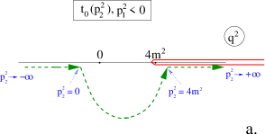
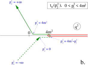
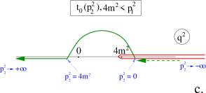
Fig. 2: The trajectory of the branch point $t_{0}(p_{1}^{2},p_{2}^{2})$ at fixed value of $p_{1}^{2}$ (which we denote as $t_{0}(p_{2}^{2})$) in the complex $q^{2}$-plane:
(a): $p_{1}^{2}\leq 0$, the (dashed-line) trajectory lies on the second sheet, and does not appear on the physical sheet; (b): $0<p_{1}^{2}<4m^{2}$: the trajectory first lies on the second sheet (dashed line), but for $p_{2}^{2}>4m^{2}-p_{1}^{2}$ moves around the normal-cut branch point through the normal cut onto the physical sheet (solid line); (c): $4m^{2}<p_{1}^{2}$: similar to case (b). The normal cut along the real axis for $q^{2}>4m^{2}$ is shown in red.

It is convenient to consider three different ranges of $p_{1}^{2}$: (a) For $p_{1}^{2}<0$, the trajectory lies on the second sheet for all values of $p_{2}^{2}$, and therefore the function is given by its normal dispersion representation in $q^{2}$. (b) For $0<p_{1}^{2}<4m^{2}$, the branch point $t_{0}$ moves onto the physical sheet through the normal $q^{2}$-cut if $p_{2}^{2}$ satisfies the relation $p_{1}^{2}+p_{2}^{2}>4m^{2}$. (c) For $4m^{2}<p_{1}^{2}$, the situation is similar to the case (b): for $p_{2}^{2}>0$ the branch point $t_{0}$ moves onto the physical sheet through the normal $q^{2}$-cut.

Therefore, for external momenta satisfying the relation $p_{1}^{2}>0$, $p_{2}^{2}>0$, $p_{1}^{2}+p_{2}^{2}>4m^{2}$, the integration contour in the dispersion representation for the form factor depends on the values of $p_{1}^{2}$ and $p_{2}^{2}$: the contour should be chosen such that it embraces both branch points: the normal branch point at $q^{2}=4m^{2}$ and the anomalous branch point at $q^{2}=t_{0}(p_{1}^{2},p_{2}^{2})$.

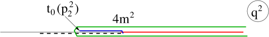
Fig. 3: The integration contour (green) in the complex $q^{2}$-plane for $0<p_{1}^{2}<4m^{2}$, $0<p_{2}^{2}<4m^{2}$, and $p_{1}^{2}+p_{2}^{2}>4m^{2}$: it embraces the anomalous cut (blue), which lies along the real axis from $t_{0}$ to $4m^{2}$, and the normal cut (red) from $4m^{2}$ to $+\infty$.

Let us consider the single dispersion representation for the form factor in the region $0<p_{1}^{2}<4m^{2}$, $0<p_{2}^{2}<4m^{2}$, and $4m^{2}<p_{1}^{2}+p_{2}^{2}$. This case corresponds to an interesting example of the relativistic two-particle bound state, and is necessary for considering the nonrelativistic expansion.

The corresponding $t_{0}$-trajectory is shown in Fig. 2(b). Fig. 3 gives the integration contour for this case: this contour may be chosen along the real axis from $t_{0}(p_{2}^{2})$ to $+\infty$. It contains two pieces: the normal part from $4m^{2}$ to $+\infty$ and the anomalous part from $t_{0}$ to $4m^{2}$.

Let us start with the normal part, which has the form

$$\sigma_{\rm norm}(t,p_{1}^{2},p_{2}^{2})=\left\{\begin{array}[]{ll}\frac{1}{16\pi\sqrt{\lambda(t,p_{1}^{2},p_{2}^{2})}}\log\left(\frac{t-p_{1}^{2}-p_{2}^{2}+\lambda^{1/2}(t,p_{1}^{2},p_{2}^{2})\sqrt{1-4m^{2}/t}}{t-p_{1}^{2}-p_{2}^{2}-\lambda^{1/2}(t,p_{1}^{2},p_{2}^{2})\sqrt{1-4m^{2}/t}}\right),&\quad(\sqrt{p_{1}^{2}}+\sqrt{p_{2}^{2}})^{2}\leq t,\\ \frac{1}{8\pi\sqrt{-\lambda(t,p_{1}^{2},p_{2}^{2})}}\arctan\left(\frac{\sqrt{-\lambda(t,p_{1}^{2},p_{2}^{2})}\sqrt{1-4m^{2}/t}}{t-p_{1}^{2}-p_{2}^{2}}\right),&\quad p_{1}^{2}+p_{2}^{2}\leq t\leq(\sqrt{p_{1}^{2}}+\sqrt{p_{2}^{2}})^{2},\\ \frac{1}{8\pi\sqrt{-\lambda(t,p_{1}^{2},p_{2}^{2})}}\left[\pi+\arctan\left(\frac{\sqrt{-\lambda(t,p_{1}^{2},p_{2}^{2})}\sqrt{1-4m^{2}/t}}{t-p_{1}^{2}-p_{2}^{2}}\right)\right],&\quad 4m^{2}\leq t\leq p_{1}^{2}+p_{2}^{2}.\end{array}\right.$$ (14)

Notice that the normal spectral density does not vanish at the normal threshold $t=4m^{2}$.

The discontinuity of the form factor $F(q^{2},p_{1}^{2},p_{2}^{2})$ on the anomalous cut is related to the discontinuity of the function $\sigma_{\rm norm}(t,p_{1}^{2},p_{2}^{2}|m^{2})$ and reads

$$\sigma_{\rm anom}(t,p_{1}^{2},p_{2}^{2})=\frac{1}{8\sqrt{-\lambda(t,p_{1}^{2},p_{2}^{2})}},\qquad t_{0}\leq t\leq 4m^{2}.$$ (15)

Therefore, the full spectral density has the form

$$\sigma(t,p_{1}^{2},p_{2}^{2})=\theta(p_{1}^{2}+p_{2}^{2}-4m^{2})\theta(t_{0}\leq t\leq 4m^{2})\sigma_{\rm anom}(t,p_{1}^{2},p_{2}^{2})+\theta(4m^{2}\leq t)\sigma_{\rm norm}(t,p_{1}^{2},p_{2}^{2}).$$ (16)

Clearly, the spectral density given by Eqs. (14) and (15) is a continuous function for $t>t_{0}$. The spectral representation for the form factor reads

$$F(q^{2},p_{1}^{2},p_{2}^{2})=\theta(p_{1}^{2}+p_{2}^{2}-4m^{2})\int\limits_{t_{0}(p_{1}^{2},p_{2}^{2})}^{4m^{2}}\frac{dt}{\pi(t-q^{2}-i0)}\sigma_{\rm anom}(t,p_{1}^{2},p_{2}^{2})+\int\limits_{4m^{2}}^{\infty}\frac{dt}{\pi(t-q^{2}-i0)}\sigma_{\rm norm}(t,p_{1}^{2},p_{2}^{2}).$$ (17)

For $t_{0}(p_{1}^{2},p_{2}^{2})<q^{2}<4m^{2}$ (in case $p_{1}^{2}+p_{2}^{2}>4m^{2}$) the imaginary part of the form factor comes from the anomalous part, while for $q^{2}>4m^{2}$ it comes from the normal part.

II.2 Double dispersion representation in $p_{1}^{2}$ and $p_{2}^{2}$

For $q^{2}\leq 0$, the triangle diagram may be written as the double dispersion representation

$$F(q^{2},p_{1}^{2},p_{2}^{2})=\int\frac{ds_{1}}{\pi(s_{1}-p_{1}^{2}-i0)}\frac{ds_{2}}{\pi(s_{2}-p_{2}^{2}-i0)}\Delta(q^{2},s_{1},s_{2}).$$ (18)

The double spectral density $\Delta(q^{2},s_{1},s_{2})$ may be obtained by placing all particles in the loop on the mass shell and taking the off-shell external momenta $p_{1}\to\tilde{p}_{1}$, $p_{2}\to\tilde{p}_{2}$, such that $\tilde{p}_{1}^{2}=s_{1}$, $\tilde{p}_{2}^{2}=s_{2}$, and $(\tilde{p}_{1}-\tilde{p}_{2})^{2}=q^{2}$ is fixed anisovich :

$$\Delta(q^{2},s_{1},s_{2}) = \frac{1}{8\pi}\int dk_{1}dk_{2}dk_{3}\delta(\tilde{p}_{1}-k_{2}-k_{3})\delta(\tilde{p}_{2}-k_{3}-k_{1})\theta(k_{1}^{0})\delta(k^{2}_{1}-m^{2})\theta(k_{2}^{0})\delta(k^{2}_{2}-m^{2})\theta(k_{3}^{0})\delta(k^{3}_{2}-m^{2}),$$ (19)

$$\quad\tilde{p}_{1}^{2}=s_{1},\quad\tilde{p}_{2}^{2}=s_{2},\quad(\tilde{p}_{1}-\tilde{p}_{2})^{2}=q^{2}.$$

Explicitly, one finds

$$\Delta(q^{2},s_{1},s_{2})=\frac{1}{16\lambda^{1/2}(s_{1},s_{2},q^{2})}\theta\left({s_{1}-4m^{2}}\right)\theta\left({s_{2}-4m^{2}}\right)\theta\left[{\left(q^{2}(s_{1}+s_{2}-q^{2})\right)^{2}-\lambda(s_{1},s_{2},q^{2})\lambda(q^{2},m^{2},m^{2})}\right].$$ (20)

The solution of the $\theta$-function gives the following allowed intervals for the integration variables $s_{1}$ and $s_{2}$:

$$4m^{2}< s_{2},$$

$$s_{1}^{-}(s_{2},q^{2})< s_{1} <s_{1}^{+}(s_{2},q^{2}),$$ (21)

where

$$s_{1}^{\pm}(s_{2},q^{2}) = s_{2}+q^{2}-\frac{s_{2}q^{2}}{2m^{2}}\pm\frac{\sqrt{s_{2}(s_{2}-4m^{2})}\sqrt{q^{2}(q^{2}-4m^{2})}}{2m^{2}}.$$ (22)

The final double dispersion representation for the triangle diagram at $q^{2}<0$ takes the form

$$F(q^{2},p_{1}^{2},p_{2}^{2})=\int\limits^{\infty}_{4m^{2}}\frac{ds_{2}}{\pi(s_{2}-p_{2}^{2}-i0)}\int\limits^{s_{1}^{+}(s_{2},q^{2})}_{s_{1}^{-}(s_{2},q^{2})}\frac{ds_{1}}{\pi(s_{1}-p_{1}^{2}-i0)}\frac{1}{16\lambda^{1/2}(s_{1},s_{2},q^{2})}.$$ (23)

Notice the relation $s_{1}^{-}(s_{2},q^{2})>4m^{2}$, which holds for all $s_{2}>4m^{2}$ at $q^{2}<0$: this guarantees that the integration region in $s_{1}$ always remains above the normal threshold. Clearly, the integration region does not depend on the values of $p_{1}^{2}$ and $p_{2}^{2}$. Essential for us is that no anomalous cuts emerge in the double dispersion representation in $p_{1}^{2}$ and $p_{2}^{2}$ for $q^{2}<0$. This makes the double dispersion representation particulary convenient for treating the triangle diagram for values of $p_{1}^{2}$ and $p_{2}^{2}$ above the thresholds. One should just take care about the appearance of the absorptive parts.

III Double spectral representation for the decay kinematics

Now we discuss the triangle diagram with particles of different masses in the loop, $m<\mu$, and consider the decay kinematics $0<q^{2}<(\mu-m)^{2}$. We have in mind the application to processes corresponding to the overthreshold values $p_{1}^{2}>(\mu+m)^{2}$ and $p_{2}^{2}>4m^{2}$, such as, e.g., the $K\to 3\pi$ decay k3pi . As we have seen in the previous section, the single dispersion representation in $q^{2}$ is rather complicated for $p_{1}^{2}$ and $p_{2}^{2}$ above the two-particle thresholds already for equal masses in the loop. The situation is much worse for unequal masses in the loop. On the other hand, we shall see that the double spectral representation in $p_{1}^{2}$ and $p_{2}^{2}$ is rather simple in this case for $q^{2}<(\mu-m)^{2}$. We start from the region $q^{2}<0$, where the double dispersion representation has the standard form both for equal and unequal masses in the loop. We then perform the analytic continuation in $q^{2}$ and observe the appearance of the anomalous contribution in the double spectral representation.

III.1 Transition form factor at $q^{2}<0$

For $q^{2}<0$, the double dispersion representation has a form very similar to the case of equal masses melikhov :

$$F(q^{2},p_{1}^{2},p_{2}^{2})=\int\limits^{\infty}_{4m^{2}}\frac{ds_{2}}{\pi(s_{2}-p_{2}^{2})}\int\limits^{s_{1}^{+}(s_{2},q^{2})}_{s_{1}^{-}(s_{2},q^{2})}\frac{ds_{1}}{\pi(s_{1}-p_{1}^{2})}\frac{1}{16\lambda^{1/2}(s_{1},s_{2},q^{2})},$$ (24)

where

$$s_{1}^{\pm}(s_{2},q^{2}) = \frac{s_{2}(m^{2}+\mu^{2}-q^{2})+2m^{2}q^{2}}{2m^{2}}\pm\frac{\lambda^{1/2}(s_{2},m^{2},m^{2})\lambda^{1/2}(q^{2},\mu^{2},m^{2})}{2m^{2}}.$$ (25)

A new feature compared with the case of equal masses in the loop is the appearance of the region $0<q^{2}<(\mu-m)^{2}$, which was absent in the equal-mass case. This region corresponds to the decay of a particle of mass $\mu$ to a particle of mass $m$ with the emission of a particle of mass $\sqrt{q^{2}}$.

III.2 Transition form factors at $q^{2}>0$

The form factor in the region $0<q^{2}<(\mu-m)^{2}$ may be obtained by analytic continuation of the expression (23). Let us consider the structure of the singularities of the integrand in Eq. (24) in the complex $s_{1}$-plane for a fixed real value of $s_{2}$ in the interval $s_{2}>4m^{2}$.

Fig. 4: Singularities of the function $\Delta(q^{2},s_{1},s_{2})$ in the complex $s_{1}$ plane as a function of $s_{2}$ for $q^{2}>0$. (This corresponds to an external $s_{2}$ and an internal $s_{1}$ integration). The trajectory $s_{1}^{R}(s_{2})$ at fixed $q^{2}>0$ is shown: for $s_{2}<s_{2}^{0}$ the branch point $s_{1}^{R}(s_{2})$ remains on the unphysical sheet (dashed line), but, as soon as $s_{2}>s_{2}^{0}$, it goes onto the physical sheet and moves to the left from the left boundary of the normal cut $s_{1}^{-}$. Respectively, for $s_{2}<s_{2}^{0}$ the integration contour in the complex $s_{1}$-plane may be chosen along the interval $[s_{1}^{-},s_{1}^{+}]$. For $s_{2}>s_{2}^{0}$, however, the contour should embrace the point $s_{1}^{R}$, and therefore the inegration contour contains two segments: the “anomalous” segment from $s_{1}^{R}$ to $s_{1}^{-}$, and the “normal” segment from $s_{1}^{-}$ to $s_{1}^{+}$.

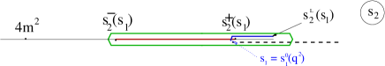
Fig. 5: Singularities of the function $\Delta(q^{2},s_{1},s_{2})$ in the complex $s_{2}$ plane as a function of $s_{1}$ for $q^{2}>0$. (This corresponds to an external $s_{1}$ and an internal $s_{2}$ integration). The trajectory $s_{2}^{L}(s_{1})$ at fixed $q^{2}>0$ is shown: for $s_{1}<s_{1}^{0}$ the branch point $s_{2}^{L}(s_{1})$ remains on the unphysical sheet (dashed line), but, as soon as $s_{1}>s_{1}^{0}$, it goes onto the physical sheet and moves to the right from the right boundary of the normal cut $s_{2}^{+}$. The notations are self-evident.

The integrand has singularities (branch points) related to the zeros of the function $\lambda(s_{1},s_{2},q^{2})$ at $s_{1}^{L}=(\sqrt{s_{2}}-\sqrt{q^{2}})^{2}$ and $s_{1}^{R}=(\sqrt{s_{2}}+\sqrt{q^{2}})^{2}$. As $q^{2}\leq 0$, these singularities lie on the unphysical sheet. However, as $q^{2}$ becomes positive, the point $s_{1}^{R}$ may move onto the physical sheet through the cut from $s_{1}^{-}$ to $s_{1}^{+}$. This happens for values of the variable $s_{2}>s_{2}^{0}$, with $s_{2}^{0}$ obtained as the solution to the equation $s_{1}^{R}(s_{2},q^{2})=s_{1}^{-}(s_{2},q^{2})$. Explicitly, one finds

$$\sqrt{s_{2}^{0}}=\frac{\mu^{2}-m^{2}-q^{2}}{\sqrt{q^{2}}}.$$ (26)

The trajectory of the point $s_{1}^{R}(s_{2},q^{2})$ in the complex $s_{1}$-plane at fixed $q^{2}>0$ vs. $s_{2}$ is shown in Fig. 4. As $q^{2}>0$, for $s_{2}>s_{2}^{0}(q^{2})$ the integration contour in the complex $s_{1}$-plane should be deformed such that it embraces the points $s_{1}^{R}$ and $s_{1}^{+}$. Respectively, the $s_{1}$-integration contour contains the two segments: the normal part from $s_{1}^{-}$ to $s_{1}^{+}$, and the anomalous part from $s_{1}^{R}$ to $s_{1}^{-}$. The double spectral density for the anomalous piece is just the discontinuity of the function $1/\sqrt{\lambda(s_{1},s_{2},q^{2})}$. It can be easily calculated as follows: Recall the relation $\sqrt{\lambda(s_{1},s_{2},q^{2})}=\sqrt{s_{1}-s_{1}^{L}}\sqrt{s_{1}-s_{1}^{R}}$. The branch point $s_{1}^{L}$ lies on the unphysical sheet, therefore the function $\sqrt{s_{1}-s_{1}^{L}}$ is continuous on the anomalous cut located on the physical sheet. Thus we have to calculate the discontinuity of the function $1/\sqrt{s_{1}-s_{1}^{R}}$ which is just twice the function itself. As the result, the discontinuity of the function $1/\sqrt{\lambda(s_{1},s_{2},q^{2})}$ on the anomalous cut is just $2/\sqrt{\lambda(s_{1},s_{2},q^{2})}$. Finally, the full double spectral density including the normal and the anomalous pieces takes the form

$$\Delta(q^{2},s_{1},s_{2}|\mu,m,m) = \frac{\theta(s_{2}-4m^{2})\theta(s_{1}^{-}<s_{1}<s_{1}^{+})}{16\lambda^{1/2}(s_{1},s_{2},q^{2})}+\frac{2\theta(q^{2})\theta(s_{2}-s_{2}^{0})\theta(s_{1}^{R}<s_{1}<s_{1}^{-})}{16\lambda^{1/2}(s_{1},s_{2},q^{2})}.$$ (27)

The first term in (27) relates to the Landau-type contribution emerging when all intermediate particles go on mass shell, while the second term describes the anomalous contribution.

The result (27) for $\Delta$ holds for $\mu>m$ implying the “external” $s_{2}$-integration, and the “internal” $s_{1}$-integration. The location of the integration region for this case is shown in Fig. 4. Fig. 5 gives the integration contour in the complex $s_{2}$ plane for the opposite order of the integrations.

The final representation for the form factors at $0<q^{2}<(\mu-m)^{2}$ takes the form

$$F(q^{2},p_{1}^{2},p_{2}^{2}) = \int\limits_{4m^{2}}^{\infty}\frac{ds_{2}}{\pi(s_{2}-p_{2}^{2}-i0)}\int\limits_{s_{1}^{-}(s_{2},q^{2})}^{s_{1}^{+}(s_{2},q^{2})}\frac{ds_{1}}{\pi(s_{1}-p_{1}^{2})}\frac{1}{16\lambda^{1/2}(s_{1},s_{2},q^{2})}$$ (28)

$$+ 2\theta\left(0<q^{2}<(\mu-m)^{2}\right)\int\limits_{s_{2}^{0}(q^{2})}^{\infty}\frac{ds_{2}}{\pi(s_{2}-p_{2}^{2}-i0)}\int\limits_{s_{1}^{R}(s_{2},q^{2})}^{s_{1}^{-}(s_{2},q^{2})}\frac{ds_{1}}{\pi(s_{1}-p_{1}^{2})}\frac{1}{16\lambda^{1/2}(s_{1},s_{2},q^{2})}.$$

A typical behavior of the anomalous and the normal contributions is plotted in Fig. 6: the normal contribution first rises at small values of $q^{2}$ but then drops down steeply and vanishes at zero recoil. The anomalous contribution is zero at $q^{2}=0$, remains small at small $q^{2}>0$, but rises steeply near zero recoil, providing a smooth behavior of the full form factor.

Fig. 6: A typical behavior of the function $F(q^{2},p_{1}^{2},p_{2}^{2})$ vs. $q^{2}$ for $0<q^{2}<(\mu-m)^{2}$ at fixed $p_{1}^{2}$ and $p_{2}^{2}$. The parameters are chosen such that $(\mu-m)^{2}=1$ GeV². Dashed: normal part, solid: anomalous part, dotted: full function (sum of both parts).

We point out that the representation (28) is particularly suitable for application to processes where $p_{1}^{2}$ and $p_{2}^{2}$ are above two-particle thresholds: in this case the single spectral representation in $q^{2}$ becomes extremely complicated, with a nontrivial integration contour in the complex $q^{2}$-plane, whereas the double dispersion representation in $p_{1}^{2}$ and $p_{2}^{2}$ has the simple form given above. For values of $p_{1}^{2}$ and $p_{2}^{2}$ above the thresholds one just has to take into account the appearance of the absorptive parts in the $s_{1}$ and $s_{2}$ integrals. A possible application of this representation may be the calculation of the triangle-diagram contribution to the three-body decay anisovich_anselm , e.g., to the $K\to 3\pi$ decay k3pi , Fig. 7. In this case the diagram with the pion loop may be represented as the $\mu^{2}$ integral of the triangle diagram considered here, and one obtains the expression for the values $p_{1}^{2}=M_{K}^{2}>9m_{\pi}^{2}$, $p_{2}^{2}>4m_{\pi}^{2}$, and $q^{2}=m_{\pi}^{2}$. The emerging absorptive parts may then be easily calculated from the double spectral representation. The problem would be technically very involved if one uses the single spectral representation in $q^{2}$, as can be seen from the complicated structure of the integration contour in Section II.

Fig. 7: The triangle-diagram contribution to the $K\to 3\pi$ amplitude may be reduced to the integral over $\mu^{2}$ of the diagram $F$.

IV The nonrelativistic expansion for the case of decay kinematics

In this section we perform the nonrelativistic expansion of the double spectral representation for the triangle diagram $F$ for the case $\mu>m$ and compare it with the triangle diagram of the nonrelativistic field theory $F_{\rm NR}$. For the latter we also obtain a double spectral representation. However, the double spectral representations for $F$ and $F_{\rm NR}$ have rather different properties. Nevertheless, the two expressions are shown to match to each other.

IV.1 Nonrelativistic expansion of the relativistic triangle diagram

Let us look at the behavior of the anomalous and the normal contributions in the NR limit. To this end, we introduce new variables: instead of $p_{1}^{2}=M_{1}^{2}$, we use $M_{1}=\mu+m-\epsilon_{1}$, instead of $p_{2}^{2}=M_{2}^{2}$, we use $M_{2}=2m-\epsilon_{2}$, and the NR approximation requires $\epsilon_{i}\ll m,\mu$. Instead of $q^{2}$, we use the variable $u$ defined by

$$q^{2}=(\mu-m)^{2}-2m(\mu+m)u^{2}.$$ (29)

The maximal decay momentum transfer $q^{2}=(\mu-m)^{2}$ corresponds to $u=0$, and the decay region is $u>0$. The meaning of the coefficient $2m(\mu+m)$ will be clear from comparison with the NR field theory. The consistency of the NR approximation requires the momentum transfer to be limited, therefore

$$u^{2}\leq O(\Lambda/m),$$ (30)

where $\Lambda$ is a constant which does not scale with the mass. In the NR limit, one finds

$$F_{\rm norm}(u,\epsilon_{1},\epsilon_{2}) = \frac{1}{64\pi^{2}\sqrt{m(\mu+m)(\mu-m)}}\int_{0}^{\infty}\frac{dz_{2}}{(z_{2}+\epsilon_{2})}\int_{z_{1}^{-}}^{z_{1}^{+}}\frac{dz_{1}}{(z_{1}+\epsilon_{1})\sqrt{z_{1}-z_{1}^{R}}},$$ (31)

$$F_{\rm anom}(u,\epsilon_{1},\epsilon_{2}) = \frac{1}{32\pi^{2}\sqrt{m(\mu+m)(\mu-m)}}\int_{z_{2}^{0}}^{\infty}\frac{dz_{2}}{(z_{2}+\epsilon_{2})}\int_{z_{1}^{R}}^{z_{1}^{-}}\frac{dz_{1}}{(z_{1}+\epsilon_{1})\sqrt{z_{1}-z_{1}^{R}}}.$$ (32)

The condition $\theta(0<q^{2}<(\mu-m)^{2})$, which defines the region where the anomalous contribution is nonvanishing, takes the form $z_{2}\leq m$. The latter condition is automatically fulfilled in the NR limit which requires $z_{1,2}\ll m$.

The integration limits

$$z_{2}^{0}=\frac{2\mu m(\mu+m)}{(\mu-m)^{2}}u^{2},\qquad z_{1}^{R}=z_{2}-\frac{2\mu}{(\mu-m)}u^{2},\qquad z_{1}^{\pm}=\frac{2\mu}{(\mu+m)}\left(\sqrt{z_{2}}\pm u\sqrt{\frac{m(\mu+m)}{2\mu}}\right)^{2}$$ (33)

are obtained by keeping the leading nonrelativistic terms of the values $s_{2}^{0}$, $s_{1}^{R}$, and $s_{1}^{\pm}$, respectively. Interestingly, both the normal and the anomalous contributions remain finite in the NR limit. Moreover, in the NR limit the normal part contains only the odd powers of $u$, whereas the terms of odd powers in $u$ cancel in the sum of the normal and the anomalous parts. Therefore, the only role of $F_{\rm norm}$ in the case of the decay kinematics is to cancel the terms of the odd powers in $u$. Recall that this is completely different from the case of the elastic kinematics: in the latter case the anomalous part is absent at all.

It is convenient to obtain the form factor as an expansion in powers of $u$ and $h$, where $h=(\mu-m)/(\mu+m)$. For the sum of the normal and the anomalous parts, we find

$$F(u^{2},\epsilon_{1},\epsilon_{2},) = \frac{1}{32\pi{m}^{3/2}\left(\sqrt{\epsilon_{1}}+\sqrt{\epsilon_{2}}\right)}-h\frac{7\sqrt{\epsilon_{1}}+8\sqrt{\epsilon_{2}}}{192\pi{m}^{3/2}\left(\sqrt{\epsilon_{1}}+\sqrt{\epsilon_{2}}\right)^{2}}$$ (34)

$$+ u^{2}\left[-\frac{1}{96\pi\sqrt{m}\left(\sqrt{\epsilon_{1}}+\sqrt{\epsilon_{2}}\right)^{3}}+h\frac{13\sqrt{\epsilon_{1}}+22\sqrt{\epsilon_{2}}}{960\pi\sqrt{m}\left(\sqrt{\epsilon_{1}}+\sqrt{\epsilon_{2}}\right)^{4}}\right]+\cdots$$

IV.2 Triangle diagram in nonrelativistic field theory

Let us first set up the nonrelativistic kinematics:

$$p_{1}^{0}=M_{1}+\frac{\vec{p}_{1}^{2}}{2M_{1}}=\mu+m-\epsilon_{1}+\frac{\vec{p}_{1}^{2}}{2(\mu+m)},\qquad p_{2}^{0}=M_{2}+\frac{\vec{p}_{2}^{2}}{2M_{2}}=2m-\epsilon_{2}+\frac{\vec{p}_{2}^{2}}{4m},$$ (35)

where we have neglected terms of order $O((\vec{p}^{2})^{2}/m^{4})$ and $O(\vec{p}^{2}\epsilon/m^{3})$. We now calculate the 4-momentum transfer $q^{2}=(p_{1}-p_{2})^{2}\simeq(M_{1}-M_{2})^{2}-M_{1}M_{2}(\vec{v}_{1}-\vec{v}_{2})^{2}$, where $\vec{v}_{i}=\vec{p}_{i}/M_{i}$, $i=1,2$. Thus, the NR form factor depends on the square of the three-dimensional velocity transfer $v^{2}\equiv\vec{v}^{2}$, $\vec{v}\equiv\vec{v}_{1}-\vec{v}_{2}$, which is reduced to $\vec{q}^{2}$ only in the elastic case $M_{1}=M_{2}$.

The propagator of a NR particle has the form $D^{-1}_{c}(E,\vec{k})=-2mE+\vec{k}^{2}-i0$ anisovich_book , and the NR triangle diagram reads

$$F_{\rm NR}(\vec{v}^{2},\epsilon_{1},\epsilon_{2}) = \frac{1}{(2\pi)^{4}i}\int\frac{dEd^{3}k}{(-2mE+\vec{k}^{2}-i0)(-2\mu(E_{1}-E)+(\vec{p}_{1}-\vec{k})^{2}-i0)(-2m(E_{2}-E)+(\vec{p}_{2}-\vec{k})^{2}-i0)},$$ (36)

$$E_{1}=\epsilon_{1}+\frac{\vec{p}_{1}^{2}}{2(\mu+m)},\quad E_{2}=\epsilon_{2}+\frac{\vec{p}_{2}^{2}}{4m}.$$

The $E$-integration is easily performed by closing the integration contour in the lower complex semiplane. Introducing the new integration variable $\vec{w}=\vec{k}/m$ (the velocity of the spectator particle in the diagram), we obtain

$$F_{\rm NR}(\vec{v}^{2},\epsilon_{1},\epsilon_{2}) = \frac{m}{64\pi^{3}\mu}\int\frac{d^{3}w}{\left[\frac{m(\mu+m)}{2\mu}(\vec{v}_{1}-\vec{w})^{2}+\epsilon_{1}-i0\right]\left[m(\vec{v}_{2}-\vec{w})^{2}+\epsilon_{2}-i0\right]}.$$ (37)

The last equation may be written in the form of the double spectral representation

$$F_{\rm NR}(\vec{v}^{2},\epsilon_{1},\epsilon_{2}) = \int\frac{dz_{1}}{\pi(z_{1}+\epsilon_{1}-i0)}\frac{dz_{2}}{\pi(z_{2}+\epsilon_{2}-i0)}\Delta_{\rm NR}(z_{1},z_{2},\vec{v}^{2})$$ (38)

with

$$\Delta_{\rm NR}(z_{1},z_{2},(\vec{v}_{1}-\vec{v}_{2})^{2})=\frac{m}{64\pi\mu}\int d^{3}w\delta\left(\frac{m(\mu+m)}{2\mu}(\vec{w}-\vec{v}_{1})^{2}-z_{1}\right)\delta\left(m(\vec{w}-\vec{v}_{2})^{2}-z_{2}\right).$$ (39)

Performing the integration over $d^{3}w$, we arrive at the following double spectral representation of the NR field theory:

$$F_{\rm NR}(v^{2},\epsilon_{1},\epsilon_{2}) = \frac{1}{64\pi^{2}m(\mu+m)}\int_{0}^{\infty}\frac{dz_{2}}{z_{2}+\epsilon_{2}}\int_{\tilde{z}_{1}^{-}}^{\tilde{z}_{1}^{+}}\frac{dz_{1}}{z_{1}+\epsilon_{1}}\frac{1}{v},\qquad\tilde{z}_{1}^{\pm}=\frac{(\mu+m)}{2\mu}\left(\sqrt{z_{2}}\pm v\sqrt{m}\right)^{2}.$$ (40)

The NR form factor may now be obtained in analytic form as the expansion in powers of $v^{2}$

$$F_{\rm NR}(v^{2},\epsilon_{1},\epsilon_{2})=\frac{1}{16\pi\sqrt{m}(\mu+m)\left(\sqrt{\epsilon_{1}}+\sqrt{\frac{2\mu}{\mu+m}}\sqrt{\epsilon_{2}}\right)}-\frac{\sqrt{m}}{48\pi(\mu+m)\left(\sqrt{\epsilon_{1}}+\sqrt{\frac{2\mu}{\mu+m}}\sqrt{\epsilon_{2}}\right)^{3}}v^{2}+O(v^{4}).$$ (41)

Finally, we may expand this expression in powers of $h$:

$$F_{\rm NR}(v^{2},\epsilon_{1},\epsilon_{2}) = \frac{1}{32\pi{m}^{3/2}\left(\sqrt{\epsilon_{1}}+\sqrt{\epsilon_{2}}\right)}-h\frac{3\sqrt{\epsilon_{1}}+2\sqrt{\epsilon_{2}}}{64\pi{m}^{3/2}\left(\sqrt{\epsilon_{1}}+\sqrt{\epsilon_{2}}\right)^{2}}$$ (42)

$$+ v^{2}\left[-\frac{1}{96\pi\sqrt{m}\left(\sqrt{\epsilon_{1}}+\sqrt{\epsilon_{2}}\right)^{3}}+h\frac{5\sqrt{\epsilon_{1}}+2\sqrt{\epsilon_{2}}}{192\pi\sqrt{m}\left(\sqrt{\epsilon_{1}}+\sqrt{\epsilon_{2}}\right)^{4}}\right]+\cdots$$

where $\cdots$ denote terms of higher orders in $h$ and $v^{2}$. For comparison with $F(u^{2},\epsilon_{1},\epsilon_{2})$, Eq. (34), one should take into account that the variables $u^{2}$ and $v^{2}$ differ from each other. Their relationship is obtained from the equation $q^{2}=(M_{1}-M_{2})^{2}-M_{1}M_{2}v^{2}=(\mu-m)^{2}-2m(\mu+m)u^{2}$, which gives, to the necessary NR accuracy,

$$v^{2}=u^{2}-h\frac{\epsilon_{1}-\epsilon_{2}}{m}.$$ (43)

Making use of this relation, $F_{\rm NR}(v^{2},\epsilon_{1},\epsilon_{2})$ and the NR expansion of $F(u^{2},\epsilon_{1},\epsilon_{2})$ perfectly match each other.

V Summary and Conclusions

We have presented a detailed analysis of dispersion representations for the triangle diagram, laying main emphasis on the appearance of the anomalous contributions to these representations. In some kinematic regions the properties of the triangle diagram and the amplitudes of the corresponding processes are mainly determined by the anomalous contributions. A message we would like to convey to the reader is that in many cases the double spectral representations in $p_{1}^{2}$ and $p_{2}^{2}$ provide great technical advantages compared to the use of the single representation in $q^{2}$. This is clearly the case for $p_{1}^{2}$ and $p_{2}^{2}$ above the thresholds and $q^{2}$ in the decay region $0<q^{2}<(\mu-m)^{2}$. Several actual physical problems belong to this class of problems.

The results presented in this paper are summarized below:

1. We pointed out that at spacelike momentum tranfer $q$, $q^{2}<0$, and for any values of $p_{1}^{2}$ and $p_{2}^{2}$, the double dispersion representation in $p_{1}^{2}$ and $p_{2}^{2}$ is particularly simple and contains only the normal cut. The calculation of the triangle diagram in this case may be easily done for all values of $p_{1}^{2}$ and $p_{2}^{2}$, including the values above the thresholds and complex values. In the same situation, the single spectral representation in $q^{2}$ contains, in addition, the anomalous cut, making the application of the single dispersion representation a very involved problem.

2. For the decay kinematics $0<q^{2}<(\mu-m)^{2}$, we presented a new derivation of the anomalous contribution to the double spectral representation. The presented approach allows an extension of double spectral representations also to higher momentum tranfers $q^{2}>(\mu+m)^{2}$.

In the decay region $0<q^{2}<(\mu-m)^{2}$, the double spectral representation in $p_{1}^{2}$ and $p_{2}^{2}$ is shown to provide a very convenient tool for considering processes at $p_{1}^{2}$ and $p_{2}^{2}$ above the thresholds. The application of the single spectral representation in $q^{2}$ faces in this case severe technical problems.

3. We analysed the double spectral representation of the triangle diagram in the region near the thresholds in $p_{1}^{2}$ and $p_{2}^{2}$ and for $q^{2}\simeq(\mu-m)^{2}$, where the nonrelativistic expansion is possible. We have shown that in this case both the normal and the anomalous contributions in $F$ are of the same order in the nonrelativistic power counting. We also constructed the double dispersion representation of the triangle diagram of the nonrelativistic field theory, $F_{\rm NR}$, and demonstrated that this representation does not contain the anomalous contribution. Nevertheless, in spite of the complications in the decay region related to the appearance of the new scale $(\mu-m)^{2}$, the $F_{\rm NR}$ and the nonrelativistic limit of $F$ are shown to match each other.