Contribution of $DK$ Continuum in the QCD Sum Rule for $D_{sJ}(2317)$

Abstract

Using the soft-pion theorem and the assumption on the final-state interactions, we include the contribution of $DK$ continuum into the QCD sum rules for $D_{sJ}(2317)$ meson. We find that this contribution can significantly lower the mass and the decay constant of $D_{s}(0^{+})$ state. For the value of the current quark mass $m_{c}(m_{c})=1.286~{}{\rm GeV}$, we obtain the mass of $D_{s}(0^{+})$ $M=2.33\pm 0.02~{}{\rm GeV}$ in the interval $s_{0}=7.5-8.0~{}{\rm GeV}^{2}$, being in agreement with the experimental data, and the vector current decay constant of $D_{s}(0^{+})$ $f_{0}=0.128\pm 0.013~{}{\rm GeV}$, much lower than those obtained in previous literature.

I Introduction

In 2003 BaBar Collaboration discovered a positive-parity scalar charm strange meson $D_{sJ}(2317)$ with a very narrow width babar , which was confirmed by CLEO cleo later. In the same experiment CLEO also observed the $1^{+}$ partner state at $2460~{}{\rm MeV}$ cleo . Since these two states lie below the $DK$ and $D^{\ast}K$ threshold, respectively, the potentially dominant s-wave decay modes $D_{sJ}(2317)\to DK$ etc., are kinematically forbidden. Thus the radiative decays and isospin-violating strong decays become the dominant decay modes. Therefore both of them are very narrow.

The discovery of these two states has triggered heated discussion on their nature in literature. The key point is to understand their low masses. The mass of $D_{sJ}(2317)$ is significantly lower than the expected values in the range of $2.4-2.6~{}{\rm GeV}$ within quark models qm . The model using the heavy-quark mass expansion of the relativistic Bethe-Salpeter equation predicted a lower value $2.369~{}{\rm GeV}$ jin , which is still higher than the experimental data by about $50~{}{\rm MeV}$.

From the experience with $a_{0}/f_{0}(980)$, Van Beveren and Rupp rupp argued that the low mass of $D_{sJ}(2317)$ could arise from the mixing between the $0^{+}$ $\bar{c}s$ state and the $DK$ continuum. In this way the lowest $0^{+}$ state could be pushed much lower than that expected from the quark models.

The mass of $D_{s}(0^{+})$ state from the lattice QCD calculation is also significantly larger than the experimentally observed mass of $D_{sJ}(2317)$ bali ; dougall ; soni . It is also pointed out in Ref. bali that $D_{sJ}(2317)$ might receive a large component of $DK$ continuum, which makes the lattice simulation very difficult.

The difficulty with the $\bar{c}s$ interpretation leads many authors to speculate that $D_{sJ}(2317)$ is a $\bar{c}qs\bar{q}$ four quark state cheng ; barns , or a strong $D\pi$ atom szc . However, calculations based on the quark model show that the mass of the four quark state is much larger than that of the $0^{+}$ $\bar{c}s$ state vijande ; zhang . The radiative decay of $D_{sJ}(2317)$ also favors that it is a $\bar{c}s$ state colangelo06 . Furthermore, there are two $0^{+}$ states in the four quark system and one in the two-quark system. Only one $0^{+}$ state has been found below the $2.86~{}{\rm GeV}$ resonance in the experimental search by BaBar babar06 , consistent with the $\bar{c}s$ interpretation.

This problem has been treated with QCD sum rules in the heavy quark effective theory in Ref. dai . The resulting $D_{s}(0^{+})$ mass is consistent with the experimental data within large theoretical uncertainties. However, the central value is still larger than the data by $90~{}{\rm MeV}$. Even larger result for the $D_{s}(0^{+})$ mass was obtained in the earlier work with the sum rule in full QCD colangelo91 . It has been pointed out in Ref. dai that, in the formalism of QCD sum rules, the physics of mixing with $DK$ continuum resides in the contribution of $DK$ continuum in the sum rule, and including this characteristic contribution should render the mass of $D_{s}(0^{+})$ lower.

Recently, there have been two investigations on this problem using sum rules in full QCD including the $O(\alpha_{s})$ corrections. In Ref. haya the value of the charm quark pole mass $M_{c}=1.46~{}{\rm GeV}$ is used, and the mass of $0^{+}$ $\bar{c}s$ state is found to be $100-200~{}{\rm MeV}$ higher than the experimental data. On the other hand, in Ref. narison the current quark mass $m_{c}=1.15~{}{\rm GeV}$ (corresponding to $M_{c}\simeq 1.3~{}{\rm GeV}$ to $O(\alpha_{s})$) is used, and the central value of the resulting $0^{+}$ $\bar{c}s$ mass is in agreement with the data. However, a low value of $m_{c}$ is used and the same value of the continuum threshold (denoted by $s_{0}$ below) is used for $0^{+}$ $\bar{c}s$ and $0^{-}$ $\bar{c}s$.

On the other hand, the perturbative three loop, order $\alpha_{s}^{2}$ correction to the two-point correlation function with one heavy and one massless quark has been calculated Chetyrkin:2000mq ; Chetyrkin:2001je . It turns out that in the pole mass scheme used by many previous analyses including Ref. narison ; haya , the perturbative expansion is far from converging. However, taking the quark mass in the modified minimal subtraction (${\overline{{\rm MS}}}$) scheme Bardeen:1978yd , better convergence of the higher order corrections is obtained, and thus a more reliable determination of physical quantities of the lowest lying resonances becomes feasible Jamin:2001fw .

Usually the contribution of two-particle continuum is neglected within the QCD sum rule formalism. However, because of the large s-wave coupling of $D_{s}(0^{+})DK$ colangelo95 ; zhu and the adjacency of the $D_{s}(0^{+})$ mass to the $DK$ threshold, this contribution may not be neglected in the considered case. In the present work, we shall therefore calculate this contribution and include it in the QCD sum rule. In the meantime we take into account the perturbative three loop order $\alpha_{s}^{2}$ correction and work in the ${\overline{{\rm MS}}}$ scheme. We find that the $DK$ continuum contribution indeed renders both the mass and the decay constant of $D_{s}(0^{+})$ significantly lower.

In Section II, we give a short overview of the traditional QCD sum rule for the scalar charm strange meson. Then we derive the $DK$ continuum contribution and write down the full sum rule in Section III. Finally, the numerical results and our conclusions are presented in Section IV. Some relevant formulas and expressions used in this paper are collected in Appendices.

II The traditional QCD sum rule for the scalar charm-strange meson

We consider the scalar correlation function

$$\Pi(p^{2})\;\equiv\;i\int\!dx\,e^{ipx}\,\langle 0|\,T\{\,j(x)\,j(0)^{\dagger}\}|\ 0\rangle\,,$$ (1)

where the renormalization invariant operator $j(x)$ is defined as

$$j(x)\;=\;(m_{c}-m_{s}):\!\bar{s}(x)\,c(x)\!:\,,$$ (2)

with $m_{c}$ and $m_{s}$ being the charm and strange quark current mass, respectively. Up to a subtraction polynomial in $p^{2}$, the correlation function $\Pi(p^{2})$ satisfies the following dispersion relation

$$\Pi(p^{2})\;=\;\int\limits_{0}^{\infty}\frac{\rho(s)}{(s-p^{2}-i\epsilon)}\,ds+\mbox{subtractions}\,.$$ (3)

At the quark gluon level, the spectra function $\rho(s)$ is calculable using the renormalization group improved perturbation theory in the framework of the operator product expansion (OPE). Following Jamin and Lange Jamin:2001fw , in this paper we shall adopt the ${\overline{{\rm MS}}}$ running quark mass scheme rather than the pole mass one, and take into account both the $O(\alpha_{s}^{2})$ terms in the perturbation theory obtained in Ref. Chetyrkin:2000mq ; Chetyrkin:2001je and the corrections from the light quark mass up to order $m_{s}^{4}$. In addition we have included the contribution from the four quark condensation which affects the final result for $D_{s}(0^{+})$ mass only by a few ${\rm Mev}$. For convenience, all the relevant expressions for $\rho(s)$ at the quark-gluon level, denoted by $\rho_{\rm QCD}(s)$, are summarized in Appendix A.

On the other hand, $\rho(s)$ can be phenomenologically written in terms of contributions from intermediate hadronic states. Generally, the spectral density at the hadronic level, denoted by $\rho_{\rm H}$, is taken to be the pole term of the lowest lying hadronic state plus the continuum starting from some threshold, with the latter identified with the QCD continuum

$$\frac{\rho_{\rm H}(t)}{\pi}=f_{0}^{2}M^{4}\delta(t-M^{2})+\textbf{QCD continuum}\times\theta(t-s_{0})\,,$$ (4)

where $f_{0}$ is the vector current decay constant of $0^{+}$ $\bar{c}s$ particle, analogous to $f_{\pi}=131~{}{\rm MeV}$. $M$ is the mass of this particle, and $s_{0}$ is the continuum threshold above which the hadronic spectral density is modeled by that at the quark gluon level. The recent works haya ; narison also use the above ansatz.

After making the Borel transformation to suppress the contribution of higher excited states and invoking the quark-hadron duality, one arrives at the sum rule

$$\int dt\,\frac{\rho_{\rm H}(t)}{\pi}\,\exp[-\frac{t}{M_{B}^{2}}]=\int\limits_{M_{c}^{2}}^{\infty}dt\,\frac{\rho_{\rm QCD}(t)}{\pi}\,\exp[-\frac{t}{M_{B}^{2}}]\,.$$ (5)

Following Ref. Jamin:2001fw , the lower limit of the integration in the above equation is taken to be the charm quark pole mass $M_{c}$, which can be expressed in terms of the running mass $m_{c}(\mu_{m})$ through the perturbative three-loop relation as defined in Appendix B.

III The contribution of $DK$ continuum

The contribution of two-particle continuum to the spectral density can safely be neglected in many cases, as usually done in the traditional QCD sum rule analysis. One typical example is the $\rho$ meson sum rule, where the two pion continuum is of p-wave nature. Its contribution to the spectral density is tiny and the $\rho$ pole contribution dominates.

However, there may be an exception when the $0^{+}$ particle couples strongly to the two-particle continuum via s-wave. In such case, there is no threshold suppression and the two-particle continuum contribution may be more significant. The strong coupling of the $0^{+}$ particle with the two-particle state and the adjacency of the $0^{+}$ mass to the $DK$ continuum threshold result in large coupling channel effect, which corresponds to the configuration of mixing in the formalism of quark model. In the problem under consideration, the mass of $D_{sJ}(2317)$ is only about $45~{}{\rm MeV}$ below the $DK$ threshold, and the s-wave coupling of $D_{s}(0^{+})DK$ is found to be very large colangelo95 ; zhu . Therefore, one may have to take into account the $DK$ continuum contribution carefully.

The importance of $D\pi$ continuum contribution in the sum rule for $D(0^{+})$ meson was first emphasized in Ref. shifman , based on the duality consideration in the case where the $D(0^{+})$ mass is higher than the $D\pi$ threshold. Based on the soft pion theorem, two of us also made a crude analysis of the $B\pi$ continuum contribution in the case where the $0^{+}$ particle mass is higher than the threshold zhu . In this work, we calculate the continuum contribution more carefully in the case where the $0^{+}$ particle mass is lower and very close to the two-particle continuum threshold.

Let $F(t)$ be the form-factor defined by

$$F(t)=\langle 0|\bar{c}(0)s(0)|DK\rangle\,.$$ (6)

From the large s-wave coupling of $D_{s}(0^{+})DK$ and the adjacency of the $D_{s}(0^{+})$ mass to the $DK$ threshold, one expects that in the low energy region, $F(t)$ is dominated by the product of a factor of the $D_{s}(0^{+})$ pole and a factor from the final state interactions. In the low energy region with $(m_{D}+m_{K})^{2}<t<s_{0}\leq 8~{}{\rm GeV}^{2}$ needed in our sum rule, the effect of inelastic $DK$ scattering is suppressed by the phase space. Therefore, we take the approximation to consider only the $DK$ scattering with only elastic intermediate states. It can be described by the $D_{s}(0^{+})DK$ interaction and the $DDKK$ chiral interaction in the low energy effective lagrangian, which can be represented by a series of bubble diagrams shown in Fig. 1.

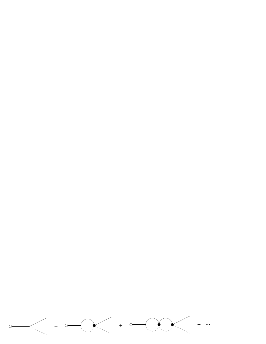
Figure 1: Heavy, light, and dotted lines represent $D_{s}(0^{+})$, $D$, and $K$, respectively. Black circle represents the Born s-wave amplitude of $DK$ scattering, and blank one the scalar current.

The s-wave Born amplitude of $DK$ scattering represented by the black circles in Fig. 1 contains three terms. The first one is the $t$ channel pole term $\frac{-ig_{0}^{2}}{t-M_{0}^{2}}$, with $g_{0}$ being the $D_{s}(0^{+})DK$ coupling constant and $M_{0}$ being the mass parameter normalized at the scale $m_{D}^{2}$ in the effective lagrangian.

The second term corresponds to the direct $DDKK$ interaction in the effective lagrangian. Let $p,k$ and $p^{\prime},k^{\prime}$ be the four momentum of $D,K$ mesons in the initial and final state respectively, and $s=(p-k^{\prime})^{2}=(p^{\prime}-k)^{2}$. In the chiral effective lagrangian, the amplitudes for the processes $D^{+}K^{0}\rightarrow D^{+}K^{0}$, $D^{0}K^{+}\rightarrow D^{0}K^{+}$, and $D^{+}K^{0}\leftrightarrow D^{0}K^{+}$ in the low energy $k_{0}$ region of $K$ meson needed in the QCD sum rule are all equal to

$$\frac{i}{2}\int\limits_{-1}^{+1}{d\cos\theta}\,\frac{t-s}{2f_{K}^{2}}=\frac{i}{2f_{K}^{2}}\Big{[}2\sqrt{t}(k_{0}+k^{\prime}_{0})-2k_{0}k^{\prime}_{0}-k^{2}-k^{\prime 2}\Big{]}\,,$$ (7)

in the center of mass system. Here $k$ and $k^{\prime}$ should be separately included in the integrals for two adjacent loops.

The third term of the s-wave Born amplitude arises from the crossing $s$ channel pole term

$$-i\frac{g_{0}^{2}}{2}\int\limits_{-1}^{+1}{d\cos\theta}\,\frac{1}{s-M_{0}^{2}}=i\frac{g_{0}^{2}}{2}\,\frac{1}{B}\,\ln{\frac{A-B}{A+B}}\,,$$ (8)

where

$$A=t-2\sqrt{t}(k_{0}+k^{\prime}_{0})+2k_{0}k^{\prime}_{0}+2m_{K}^{2}-M_{0}^{2},\qquad B=2|\vec{k}||\vec{k^{\prime}}|\,.$$ (9)

For simplicity, we put the on-shell values of $k_{0}$, $k^{\prime}_{0}$, $|\vec{k}|$, $|\vec{k^{\prime}}|$ into $A$ and $B$ in the above equations. The effect of this approximation on our final results is expected to be small, since the contribution of the $s$ channel pole term is relatively small. As a result, one finds that the $s$ channel pole term is an analytic function of $t$ with only a short cut, the length of which is only $0.146~{}{\rm GeV}^{2}$ for experimental values of the corresponding masses. Therefore, it can be well approximated by a pole form $-i\frac{cg_{0}^{2}}{t-t_{0}}$, where

$$t_{0}={{1\over 2}\,\left[\,2m_{D}^{2}+2m_{K}^{2}-M_{0}^{2}+\frac{(m_{D}^{2}-m_{K}^{2})^{2}}{M_{0}^{2}}\,\right]}\,,$$ (10)

$$c={{2m_{D}^{2}+2m_{K}^{2}-M_{0}^{2}-{(m_{D}^{2}-m_{K}^{2})^{2}\over M_{0}^{2}}}\over{{(m_{D}^{2}-m_{K}^{2})^{2}\over t_{0}}+t_{0}-2m_{D}^{2}-2m_{K}^{2}}}\,.$$ (11)

With the above results for the three terms of the s-wave Born amplitude, we can now evaluate the sum of the series of the bubble diagrams shown in Fig. 1. Let $f_{n}(t)$ be the partial sum of the series of loop diagrams in Fig. 1, with the loop number less or equal to $n$. It can then be written in the form

$$f_{n}(t)=\frac{-1}{2f_{K}^{2}}\,\bigg{\{}\Big{[}(2\sqrt{t}\,k^{\prime}_{0}-k^{\prime 2})-2f_{K}^{2}(\frac{g_{0}^{2}}{t-M_{0}^{2}}+\frac{cg_{0}^{2}}{t-t_{0}})\Big{]}\,f_{n0}+2\,(\sqrt{t}-k^{\prime}_{0})\,f_{n1}-f_{n2}\bigg{\}}\,,$$ (12)

where $k^{\prime}_{0}$ and $k^{\prime}$ is the energy and momentum of final-state $K$ meson, and the three unknown functions $f_{ni}$ ($i=0,1,2$) correspond to the diagrams with a factor $1$, $k_{0}$, and $k^{2}$ respectively at the last vertex, which contributes to the integration over the last loop of each diagram.

Let $\Sigma_{i}(t)$ be integrals defined by Eqs.(C1)-(C6) which appear as the loop integrals of the individual loop diagrams shown in Fig. 1. They can be evaluated using dimensional regularization DR , with the corresponding analytic results given in (C1)-(C6). A recurrence relations can be written between $f_{n}(t)$ and $f_{(n+1)}(t)$, and hence between $f_{ni}(t)$ and $f_{(n+1)i}(t)$, the coefficients of which are linear combinations of the loop-integral functions $\Sigma_{i}(t)$. Taking the limit $\lim_{n\rightarrow\infty}f_{ni}(t)=f_{i}(t)$, $\lim_{n\rightarrow\infty}f_{n}(t)=f(t)$ and separating out terms with the factor $1$, $k^{\prime}_{0}$, and $k^{\prime 2}$, we can obtain a system of three linear equations for the three unknown functions $f_{i}(t)$

$$2\,f_{1}\,\Sigma_{4}+f_{0}\,\Sigma_{5}-2\,\Big{[}f_{1}\,\left(2\,\Sigma_{2}+\Sigma_{3}\right)+2\,f_{0}\,\Sigma_{4}\Big{]}\,{\sqrt{t}}+4\,\left(f_{1}\,\Sigma_{1}+f_{0}\,\Sigma_{2}\right)\,t$$

$$+4\,f_{K}^{4}\,g_{0}^{2}\,\Big{[}g_{0}\,\Sigma_{0}-f_{0}\,\left(M_{0}^{2}+g_{0}^{2}\,\Sigma_{0}-t\right)\Big{]}\,\Big{[}\frac{c}{{\left(t-t_{0}\right)}^{2}}+\frac{1}{\left(t-M_{0}^{2}\right)\,\left(t-t_{0}\right)}\Big{]}\,$$

$$+2\,f_{K}^{2}\,\frac{g_{0}\,\left(1-2\,f_{0}\,g_{0}\right)\,\left(2\,\Sigma_{1}\,{\sqrt{t}}-\Sigma_{3}\right)+2\,f_{1}\,\Big{[}g_{0}^{2}\,\Sigma_{1}-\left(M_{0}^{2}+g_{0}^{2}\,\Sigma_{0}\right)\,{\sqrt{t}}+t^{\frac{3}{2}}\Big{]}}{t-M_{0}^{2}}\,$$

$$+f_{2}\,\bigg{[}\Sigma_{3}-2\,\Sigma_{1}\,{\sqrt{t}}+2\,f_{K}^{2}\,g_{0}^{2}\,\Sigma_{0}\,\left(\frac{1}{t-M_{0}^{2}}+\frac{c}{t-t_{0}}\right)-2\,f_{K}^{2}\bigg{]}\,$$

$$+2\,f_{K}^{2}\,\frac{2\,c\,g_{0}^{2}\,\Big{[}f_{1}\,\Sigma_{1}+f_{0}\,\Sigma_{3}-\left(f_{1}\,\Sigma_{0}+2\,f_{0}\,\Sigma_{1}\right)\,{\sqrt{t}}\Big{]}\,}{t-t_{0}}\,$$

$$+4\,c\,f_{0}\,f_{K}^{4}\,g_{0}^{4}\,\Sigma_{0}\,\Big{[}\frac{c}{{\left(t-t_{0}\right)}^{2}}+\frac{1}{\left(t-M_{0}^{2}\right)\,\left(t-t_{0}\right)}\Big{]}=0\,,$$ (13)

$$f_{2}\,\Sigma_{1}+f_{0}\,\Sigma_{4}-\Big{[}f_{2}\,\Sigma_{0}+f_{0}\,\left(2\,\Sigma_{2}+\Sigma_{3}\right)\Big{]}\,{\sqrt{t}}+2\,f_{1}\,\left(-f_{K}^{2}+\Sigma_{2}-2\,\Sigma_{1}\,{\sqrt{t}}+\Sigma_{0}\,t\right)\,$$

$$+2\,f_{K}^{2}\,\frac{g_{0}\,\left(1-f_{0}\,g_{0}\right)\,\Sigma_{1}+\Big{[}f_{0}\,M_{0}^{2}-g_{0}\,\left(1-f_{0}\,g_{0}\right)\,\Sigma_{0}\Big{]}\,{\sqrt{t}}-f_{0}\,t^{\frac{3}{2}}}{M_{0}^{2}-t}+2\,f_{0}\,\Sigma_{1}\,t$$

$$+2\,f_{K}^{2}\,\frac{c\,f_{0}\,g_{0}^{2}\,\left(\Sigma_{1}-\Sigma_{0}\,{\sqrt{t}}\right)}{t-t_{0}}=0\,,$$ (14)

$$2\,f_{1}\,\Sigma_{1}+f_{0}\,\bigg{[}\Sigma_{3}-2\,\Sigma_{1}\,{\sqrt{t}}+2\,f_{K}^{2}\,g_{0}^{2}\,\Sigma_{0}\,\left(\frac{1}{t-M_{0}^{2}}+\frac{c}{t-t_{0}}\right)-2\,f_{K}^{2}\bigg{]}\,$$

$$+\Sigma_{0}\,\left(f_{2}-\frac{2\,f_{K}^{2}\,g_{0}}{t-M_{0}^{2}}-2\,f_{1}\,{\sqrt{t}}\right)=0\,,$$ (15)

from which the analytic forms for $f_{i}(t)$ can then be deduced. The results are shown in Eqs. (C9)-(C12).

Finally, with the explicit expressions for $f_{i}(t)$ and $\Sigma_{i}(t)$ given in Appendix C, and putting the on-shell value of $k^{\prime}$ to Eq. (12), we obtain

$$F(t) = \frac{-g_{0}}{t-M_{0}^{2}}-\frac{1}{2f_{K}^{2}}\,\bigg{\{}\Big{[}(t-m_{D}^{2})-2f_{K}^{2}(\frac{g_{0}^{2}}{t-M_{0}^{2}}+\frac{cg_{0}^{2}}{t-t_{0}})\Big{]}\,f_{0}+\frac{m_{D}^{2}-m_{K}^{2}}{\sqrt{t}}\,f_{1}-f_{2}\bigg{\}}$$ (16)

$$= {{\lambda}\over{t-M_{0}^{2}-\Delta(t)}}\,,$$

where $\Delta(t)$ is given by Eq. (57).

Similarly, with the same series of $DK$ loops included, the full propagator of $D_{s}(0^{+})$ meson is related to the function $f_{0}(t)$ through

$${\rm Prop(t)}=\frac{i}{t-M_{0}^{2}}\,\big{[}1-g_{0}f_{0}(t)\big{]}\,.$$ (17)

Using the solution for $f_{0}(t)$ obtained above and given by Eq. (53), it can be further rewritten as

$${\rm Prop(t)}=\frac{1}{t-M_{0}^{2}-\Delta_{1}(t)}\,,$$ (18)

with $\Delta_{1}(t)$ given by Eq. (58).

We have chosen the scale $\mu$ so that the mass parameter $M_{0}$ is the physical mass of $D_{s}(0^{+})$ in our approximation, i.e., $\Delta_{1}(M_{0}^{2})=0$. The bare coupling constant $g_{0}$ is related to the physical coupling constant $g$ by $g=g_{0}/\sqrt{Z}$, where

$$Z={d\over{dt}}\left[\,t-M_{0}^{2}-\Sigma(t)\,\right]_{t=M_{0}^{2}}\,,$$ (19)

is the on-shell wave function renormalization constant of $D_{s}(0^{+})$ meson.

In order to fix the unknown constant $\lambda$ in $F(t)$ given by Eq. (16), we apply the soft-pion theorem

$$F(m_{D}^{2})=\frac{f_{D}m_{D}^{2}}{f_{K}(m_{c}+m_{u})}$$ (20)

to the extrapolated value of the matrix element $\langle 0|\bar{c}(0)s(0)|DK\rangle$ at $t=m_{D}^{2}$, from which we can deduce the constant

$$\lambda=\frac{f_{D}m_{D}^{2}}{f_{K}(m_{c}+m_{u})}\,\big{[}M^{2}_{D}-M_{0}^{2}-\Delta(m_{D}^{2})\big{]}\,.$$ (21)

With all the above equipments, the $DK$ continuum contribution to the hadronic spectral function can then be written as

$$\rho_{DK}(t) \;=\; \frac{1}{8\pi^{2}}\,\sqrt{1-{(m_{D}+m_{K})^{2}\over t}}\,\sqrt{1-{(m_{D}-m_{K})^{2}\over t}}\,(m_{c}-m_{s})^{2}\,|F(t)|^{2}$$ (22)

$$\times\theta(\sqrt{t}-m_{D}-m_{K})\,\theta(s_{0}-t)\,.$$

In the above calculations we have neglected the contribution of the $D_{s}\eta$ channel. The threshold of this channel is at $t=6.329~{}{\rm GeV}^{2}$. Our formula for the contribution of the two-particle term is proportional to $(t-M_{0}^{2})^{-2}$. The lower part of the integration in $t$ is more important. At the thresholds of the two channels the factor $(t-M_{0}^{2})^{-2}$ for the $DK$ channel is about 18 times larger than that for the $D_{s}\eta$ channel. Therefore, the effect of the latter is expected to be small.

IV Numerical results and discussions

In our numerical analysis, we use the recent result for c quark current mass $m_{c}(m_{c})=1.286~{}{\rm GeV}$ Kuhn:2007vp . Other input parameters are the following  (assuming the isospin symmetry): $\alpha_{s}(m_{Z})=0.1189$ Bethke:2006ac , $m_{s}(2~{}{\rm GeV})=96.10~{}{\rm MeV}$ Narison:2005ny , $m_{u}(2~{}{\rm GeV})=m_{s}(2~{}{\rm GeV})/24.4$ Narison:2005ny , $\langle\bar{s}s\rangle=0.8\times(-0.243)^{3}~{}{\rm GeV}^{3}$ narison , $\langle\bar{s}g_{s}\sigma\cdot Gs\rangle=0.8~{}{\rm GeV}^{2}\times\langle\bar{s}s\rangle$ narison , $\langle\alpha_{s}G^{2}\rangle=0.06~{}{\rm GeV}^{4}$ narison , in the four quark condensation term Eq. (37) $\sigma=3$, $m_{D}=\frac{m_{D^{\pm}}+m_{D^{0}}}{2}=1866.9~{}{\rm MeV}$ pdg , $m_{K}=\frac{m_{K^{\pm}}+m_{K^{0}}}{2}=495.66~{}{\rm MeV}$ pdg , $f_{D}=222.6~{}{\rm MeV}$ pdg , $f_{K}=159.8~{}{\rm MeV}$ pdg .

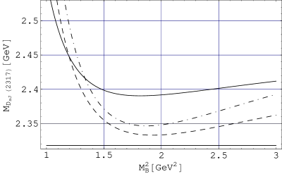
Figure 2: The variation of $M$ with $M_{B}^{2}$ when $s_{0}=8.0~{}{\rm GeV}^{2}$. The solid, dashdotted, and dashed curves are for the case without the $DK$ continuum contribution, $g=4.0~{}{\rm GeV}$, and $g=7.0~{}{\rm GeV}$, respectively.

The renormalized coupling constant $g$ was determined to be in the interval $g=5.1-7.5~{}{\rm GeV}$ in Refs. colangelo95 ; zhu . Inclusion of the contribution of $DK$ continuum in the sum rule analysis of the scalar current channel will lower the $g$ value. Since the uncertainty is large, we have not calculated this correction and simply allow the renormalized $g$ to vary in the region $g=4.0-7.0~{}{\rm GeV}$.

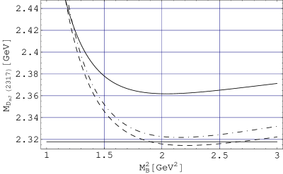
Figure 3: The variation of $M$ with $M_{B}^{2}$ when $s_{0}=7.5~{}{\rm GeV}^{2}$. The other captions are the same as in Fig. 2.

A resonance of the $D_{s}$ system with the natural parity has has been observed experimentally at $t=8.18~{}{\rm GeV}^{2}$ babar06 . If it is an excited state of $D_{s}(0^{+})$, we should confine us to $s_{0}$ smaller than and close to $8.0~{}{\rm GeV}^{2}$. We shall first consider this case and then discuss the case that this resonance is not a $0^{+}$ state. The convergence of the OPE series and dominance of the sum by the pole and the $DK$ continuum terms over the QCD continuum beyond $s_{0}$ constrain the Borel mass $M_{B}$ in a region depending on the parameters $m_{c}(m_{c})$ and $s_{0}$. Taking $m_{c}=1.286~{}{\rm GeV}$, $M_{B}^{2}\in[0.99,2.68]~{}{\rm GeV}^{2}$ for $s_{0}=8.0~{}{\rm GeV}^{2}$, and $M_{B}^{2}\in[0.99,2.41]~{}{\rm GeV}^{2}$ for $s_{0}=7.5~{}{\rm GeV}^{2}$. As mentioned in Refs. Jamin:2001fw ; Bordes:2005wi ; Bordes:2004vu , the convergence of the perturbative expansion of the two-point correlation function, when written in terms of the pole quark mass, is rather poor, the order $\alpha_{s}$ and $\alpha_{s}^{2}$ loop contributions being of similar size with, or even larger than, the leading term, while the expansion in terms of the ${\overline{{\rm MS}}}$ running mass converges much faster. However, it should be noted that, even in the ${\overline{{\rm MS}}}$ running mass scheme, the convergence of the asymptotic series in the $D_{s}$ meson system is worse than the one found in the $B_{s}$ meson system. For $D_{s}(0^{+})$ the first order correction amounts to about $53\%$ and the second order to about $47\%$ of the leading term using the values of our input parameters and $s_{0}=8.0~{}{\rm GeV}^{2}$. The same observation has also be made in Ref. Bordes:2005wi .

We first move the $DK$ continuum contribution to the right hand side of the sum rule. Then we obtain the curve of $M$ with respect to $M_{B}$ by taking the derivative of the logarithm of both sides of the sum rule as usually done. Since this curve depends on the unknown parameters $M_{0}$, we have to do it self-consistently by requiring that the $M$ value determined by the sum rule for the input “trial” value of $M_{0}$ both lies in the middle of the stability window and equals roughly to $M_{0}$. For reliability of the results we also require that the ratio of $DK$ contribution to the whole sum rule is not larger than about $60\%$.

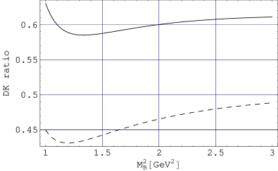
Figure 4: The ratio of the $DK$ continuum contribution as a function of $M_{B}^{2}$ with $s_{0}=8.0~{}{\rm GeV}^{2}$. The solid and dashed curves are for $g=4.0~{}{\rm GeV}$, and $g=7.0~{}{\rm GeV}$, respectively.

With the input $m_{c}(m_{c})=1.286~{}{\rm GeV}$, we present the variation of $M$ with $M_{B}^{2}$ for $s_{0}=8.0~{}{\rm GeV}^{2}$ and $s_{0}=7.5~{}{\rm GeV}^{2}$ in Figs. 2 and 3, respectively. For comparison, we also show the case without $DK$ continuum contribution with the same set of input parameters. It can be seen clearly from the two figures that the inclusion of the $DK$ continuum contribution can lower the $M$ value by $60-40~{}{\rm MeV}$. The $DK$ continuum contributes around $45\%$ to $60\%$ of the right hand side of the final sum rule for $s_{0}=8.0~{}{\rm GeV}^{2}$ as shown in Fig. 4. Another interesting point is about the vector current decay constant $f_{0}$ of $D_{s}(0^{+})$ meson. We find that the inclusion of $DK$ continuum contribution lowers the decay constant $f_{0}$ from about $0.185~{}{\rm GeV}$ to $0.115-0.132~{}{\rm GeV}$ for the same $s_{0}$ value as can be seen from Fig. 5.

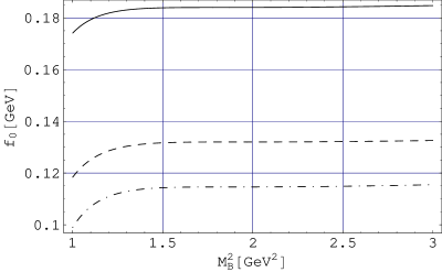
Figure 5: The vector current decay constant $f_{0}$ as a function of $M_{B}^{2}$ with $s_{0}=8.0~{}{\rm GeV}^{2}$. The other captions are the same as in Fig. 2.

For $m_{c}(m_{c})=1.286~{}{\rm GeV}$ and $s_{0}=7.5-8.0~{}{\rm GeV}^{2}$, we found $M=2.331\pm 0.016~{}{\rm GeV}$, being in agreement with the experimental data $2317.8\pm 0.6~{}{\rm MeV}$ pdg . For the same value of input parameters, we found $f_{0}=0.128\pm 0.013~{}{\rm GeV}$, which is, however, significantly lower than the ones obtained in previous literature. Here we have not included the errors due to uncertainties in the QCD sum rule except those from the variation of the results in the stability window and the $s_{0}$ interval, since our main interest is the central value of the results. The previous results already shew that the $D_{s}(0^{+})$ mass lies in the large uncertainty interval of the QCD sum rule haya ; narison .

Now we consider the case that the new resonance found in  babar06 is not a $0^{+}$ state. In this case the $s_{0}$ value can only be determined by stability analysis. The results for the mass $M$ found for $s_{0}=8.5,8.0,7.5,7.0~{}{\rm GeV}^{2}$ for $g=7~{}{\rm GeV}$ and $g=4~{}{\rm GeV}$ are shown in Fig. 6 and Fig. 7 respectively. The working region for $s_{0}=8.5~{}{\rm GeV}^{2}$ and $s_{0}=7.0~{}{\rm GeV}^{2}$ are $[0.99,2.96]~{}{\rm GeV}^{2}$ and $[0.99,2.13]~{}{\rm GeV}^{2}$ respectively. The region of the $s_{0}$ value can be chosen by requiring the least sensitivity of the results for the mass to the value of $s_{0}$. It is clear from these figures that this is the region between $s_{0}=7.5~{}{\rm GeV}^{2}$ and $s_{0}=8.0~{}{\rm GeV}^{2}$ which is just the region chosen above for the case of a $0^{+}$ resonance at $t=8.18~{}{\rm GeV}^{2}$. Also the best stability with respect to $M_{B}$ is achieved at $s_{0}=7.5~{}{\rm GeV}^{2}$. Therefore, the results obtained above are essentially unchanged.

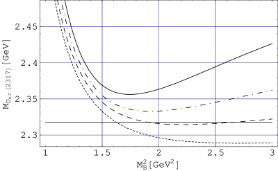
Figure 6: The variation of $M$ with $M_{B}^{2}$ when $g=7~{}{\rm GeV}^{2}$. The solid, dashdotted, dashed and dotted curves are for the case $s_{0}=8.5~{}{\rm GeV}^{2}$, $s_{0}=8.0~{}{\rm GeV}^{2}$,$s_{0}=7.5~{}{\rm GeV}^{2}$,and $s_{0}=7.0~{}{\rm GeV}^{2}$ respectively.

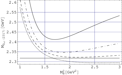
Figure 7: The variation of $M$ with $M_{B}^{2}$ when $g=4~{}{\rm GeV}^{2}$. The solid, dashdotted, dashed and dotted curves are for the case $s_{0}=8.5~{}{\rm GeV}^{2}$, $s_{0}=8.0~{}{\rm GeV}^{2}$,$s_{0}=7.5~{}{\rm GeV}^{2}$,and $s_{0}=7.0~{}{\rm GeV}^{2}$ respectively.

The above results show that the contribution of $DK$ continuum, which contains the physics of the coupled channel effect in the formalism of QCD sum rule, is significant and is partly the reason for the unexpected low mass of $0^{+}$ $\bar{c}s$ state. Our analysis also explains partly why the extracted mass of the $0^{+}$ $\bar{c}s$ state from the quenched lattice QCD simulation is higher than the experimental value where the DK continuum contribution was not included.

Acknowledgements We thank Prof. H.-Y. Cheng for beneficial discussion and Dr Chun Liu and Dr. Xiang Liu for their kind help. S.L.Z. was supported by the National Natural Science Foundation of China under Grants 10625521 and 10721063 and Ministry of Education of China.

Appendices

Appendix A The spectral function $\rho_{\rm QCD}(s)$ at the quark gluon level

In this appendix, all the relevant expressions for the spectral function $\rho(s)$ are given. For further details, we refer the readers to Ref. Jamin:2001fw and references therein.

A.1 The perturbative spectral function

In perturbation theory, the spectral function $\rho_{\rm QCD}(s)$ has an expansion in powers of the strong coupling constant

$$\rho_{\rm QCD}(s)=\rho^{(0)}(s)+\rho^{(1)}(s)\,a(\mu_{a})+\rho^{(2)}(s)\,a(\mu_{a})^{2}+\ldots\,,$$ (23)

with $a(\mu_{a})\equiv\alpha_{s}(\mu_{a})/\pi$. The leading order term $\rho^{(0)}(s)$ results from a calculation of the bare quark-antiquark loop and is given by

$$\rho^{(0)}(s)=\frac{N_{c}}{8\pi^{2}}\,(m_{c}+m_{s})^{2}\,s\,(1-\frac{m_{c}^{2}}{s})^{2}\,,$$ (24)

and, up to order $m_{s}^{4}$, the corrections in small mass $m_{s}$ can be found in Ref. Jamin:1992se

$$\rho^{(0)}_{m}(s)=\frac{N_{c}}{8\pi^{2}}\,(m_{c}+m_{s})^{2}\,\left\{2(1-x)m_{c}m_{s}-2m_{s}^{2}-2\,\frac{(1+x)}{(1-x)}\frac{m_{c}m_{s}^{3}}{s}+\frac{(1-2x-x^{2})}{(1-x)^{2}}\frac{m_{s}^{4}}{s}\,\right\}\,,$$ (25)

where $x\equiv m_{c}^{2}/s$, and the appearing quark masses correspond to the running masses in the ${\overline{{\rm MS}}}$ scheme with $m_{c}(\mu_{m})$ and $m_{s}(\mu_{m})$ evaluated at the scale $\mu_{m}$

The order $\alpha_{s}$ correction $\rho^{(1)}(s)$ can be written as

$$\rho^{(1)}(s) \!=\! \frac{N_{c}}{16\pi^{2}}\,C_{F}\,(m_{c}+m_{s})^{2}\,s\,(1-x)\biggl{\{}(1-x)\Big{[}\,4L_{2}(x)+2\ln x\ln(1-x)-\,(5-2x)$$

$$\times\ln(1-x)\,\Big{]}+(1-2x)(3-x)\ln x+3(1-3x)\ln\frac{\mu_{m}^{2}}{m_{c}^{2}}+\frac{1}{2}(17-33x)\,\biggr{\}}\,,$$ (26)

where $L_{2}(x)$ is the dilogarithmic function. The order $\alpha_{s}$ mass corrections to the spectral function can be obtained by expanding the results given by Broadhurst:1981jk ; Generalis:1990id up to order $m_{s}^{4}$, after the higher dimensional operators have been expressed in terms of non-normal ordered condensates

$$\rho^{(1)}_{m}(s) = \frac{N_{c}}{8\pi^{2}}\,C_{F}\,(m_{c}+m_{s})^{2}\,m_{c}m_{s}\,\biggl{\{}(1-x)\Big{[}\,4L_{2}(x)+2\ln x\ln(1-x)-\,2(4-x)$$

$$\times\ln(1-x)\,\Big{]}+2(3-5x+x^{2})\ln x+3(2-3x)\ln\frac{\mu_{m}^{2}}{m_{c}^{2}}+2(7-9x)\,\biggr{\}}\,,$$ (27)

$$\vbox{\vskip 34.1433pt}\rho^{(1)}_{m^{2}}(s) = -\,\frac{N_{c}}{8\pi^{2}}\,C_{F}\,(m_{c}+m_{s})^{2}\,m_{s}^{2}\,\biggl{\{}(1-x)\Big{[}\,4L_{2}(x)+2\ln x\ln(1-x)\,\Big{]}$$

$$-\,(2+x)(4-x)\ln(1-x)+(6+2x-x^{2})\ln x+6\ln\frac{\mu_{m}^{2}}{m_{c}^{2}}+(8-3x)\,\biggr{\}}\,,$$ (28)

$$\vbox{\vskip 34.1433pt}\rho^{(1)}_{m^{3}}(s) = -\,\frac{N_{c}}{8\pi^{2}}\,C_{F}\,(m_{c}+m_{s})^{2}\,\frac{m_{c}m_{s}^{3}}{s}\,\biggl{\{}\,4L_{2}(x)+2\ln x\ln(1-x)+\frac{(9+8x-9x^{2})}{(1-x)^{2}}$$

$$-\,2\frac{(7+7x-2x^{2})}{(1-x)}\ln(1-x)+2\frac{(6+7x-2x^{2})}{(1-x)}\ln x+6\frac{(2-x^{2})}{(1-x)^{2}}\ln\frac{\mu_{m}^{2}}{m_{c}^{2}}\,\biggr{\}}\,,$$ (29)

$$\vbox{\vskip 34.1433pt}\rho^{(1)}_{m^{4}}(s) = \frac{N_{c}}{8\pi^{2}}\,C_{F}\,(m_{c}+m_{s})^{2}\,\frac{m_{s}^{4}}{s}\,\biggl{\{}\,2L_{2}(x)+\ln x\ln(1-x)$$

$$-\,\frac{(13-24x-27x^{2}+2x^{3})}{2(1-x)^{2}}\ln(1-x)+\frac{(12-22x-27x^{2}+2x^{3})}{2(1-x)^{2}}\ln x$$

$$+\,3\frac{(4-12x+x^{2}+3x^{3})}{2(1-x)^{3}}\ln\frac{\mu_{m}^{2}}{m_{c}^{2}}+\frac{(6-64x+15x^{2}+11x^{3})}{4(1-x)^{3}}\,\biggr{\}}\,.$$ (30)

The three-loop, order $\alpha_{s}^{2}$ correction $\rho^{(2)}(s)$ has been calculated by Chetyrkin and Steinhauser Chetyrkin:2000mq ; Chetyrkin:2001je for the case of one heavy and one massless quark. In the present analysis, we shall make use of the program Rvs.m, which contains the required expressions for $\rho^{(2)}(s)$ Chetyrkin:2000mq ; Chetyrkin:2001je . However, since the spectral function has been calculated only in the pole mass scheme, following Jamin and Lange Jamin:2001fw , in the ${\overline{{\rm MS}}}$ scheme we still have to add to $\rho^{(2)}(s)$ the contributions resulting from rewriting the pole mass in terms of the ${\overline{{\rm MS}}}$ mass. The two contributions $\Delta_{1}\rho^{(2)}$ and $\Delta_{2}\rho^{(2)}$ which arise from the leading and first order contributions, respectively, are given by

$$\Delta_{1}\rho^{(2)}(s) = \frac{N_{c}}{8\pi^{2}}\,(m_{c}+m_{s})^{2}\,s\,\Big{[}\,(3-20x+21x^{2})\,r_{m}^{(1)^{2}}-2(1-x)(1-3x)\,r_{m}^{(2)}\,\Big{]}\,,$$ (31)

$$\vbox{\vskip 25.60747pt}\Delta_{2}\rho^{(2)}(s) \!=\! -\,\frac{N_{c}}{8\pi^{2}}\,C_{F}\,(m_{c}+m_{s})^{2}\,s\,r_{m}^{(1)}\biggl{\{}(1-x)(1-3x)\Big{[}\,4L_{2}(x)+2\ln x\ln(1-x)\,\Big{]}$$

$$-\,(1-x)(7-21x+8x^{2})\ln(1-x)+(3-22x+29x^{2}-8x^{3})\ln x$$

$$+\,\frac{1}{2}(1-x)(15-31x)\,\biggr{\}}\,,$$ (32)

where explicit expressions for the coefficients $r_{m}^{(1)}$ and $r_{m}^{(2)}$ can be found in Appendix B.

A.2 The condensate contributions

In the following, we summarize the contributions to the spectral function $\rho_{\rm QCD}(s)$ coming from higher dimensional operators, which arise in the framework of the OPE and parameterize the appearance of non-perturbative physics. Since the spectral functions corresponding to the condensates contain $\delta$-distribution contributions, we shall present directly the Borel transformed integrated quantity $u\widehat{\Pi}(u)=\int\limits_{0}^{\infty}e^{-s/u}\rho_{\rm QCD}(s)\,ds$ below, where $u=M_{B}^{2}$ with $M_{B}$ being the Borel mass.

The leading order expression for the dimension-three quark condensate is well known with the explicit form given by

$$u\widehat{\Pi}^{(0)}_{\bar{q}q}(u)=-\,(m_{c}+m_{s})^{2}m_{c}\langle\bar{q}q\rangle\,e^{-m_{c}^{2}/u}\,\left[\,1-(1+\frac{m_{c}^{2}}{u})\frac{m_{s}}{2m_{c}}+\frac{m_{c}^{2}m_{s}^{2}}{2u^{2}}\,\right]\,,$$ (33)

where the expansion up to order $m_{s}^{2}$ has been included Jamin:1992se . The first order correction to the quark condensate can be deduced based on the fact that the mass logarithms must cancel once the quark condensate is expressed in terms of the non-normal ordered condensate Jamin:1992se ; Spiridonov:1988md ; Chetyrkin:1994qu with

$$u\widehat{\Pi}^{(1)}_{\bar{q}q}(u)=\frac{3}{2}\,C_{F}\,a\,(m_{c}+m_{s})^{2}m_{c}\langle\bar{q}q\rangle\,\biggl{\{}\Gamma(0,\frac{m_{c}^{2}}{u})-\Big{[}\,1+(1-\frac{m_{c}^{2}}{u})\,(\ln\frac{\mu_{m}^{2}}{m_{c}^{2}}+\frac{4}{3})\,\Big{]}\,e^{-m_{c}^{2}/u}\,\biggr{\}}\,,$$ (34)

where $\Gamma(n,z)$ is the incomplete $\Gamma$-function.

The next contribution in the OPE is the dimension-four gluon condensate with the corresponding expression given by

$$u\widehat{\Pi}^{(0)}_{FF}(u)\;=\;\frac{1}{12}\,(m_{c}+m_{s})^{2}\,\langle aFF\rangle\,e^{-m_{c}^{2}/u}\,.$$ (35)

The dimension-five mixed quark gluon condensate should also be included, since it is enhanced by the heavy quark mass and hence still has some influence on the sum rule. Again the result is well known with

$$u\widehat{\Pi}^{(0)}_{\bar{q}Fq}(u)=-\,(m_{c}+m_{s})^{2}\,\frac{m_{c}\langle g_{s}\bar{q}\sigma Fq\rangle}{2u}\,\Big{(}1-\frac{m_{c}^{2}}{2u}\Big{)}\,e^{-m_{c}^{2}/u}\,.$$ (36)

The last condensate contribution considered in this paper is the four-quark condensate

$$u\widehat{\Pi}^{(0)}_{(\bar{s}s)^{2}}(u)=-\sigma\frac{8\pi}{27}\,\left(2-\frac{m_{c}^{2}}{2u}-\frac{m_{c}^{4}}{6u^{2}}\right)\,\alpha_{s}\langle\bar{s}s\rangle^{2},$$ (37)

where $\sigma$ is the factor representing the deviation from vacuum saturation. The contributions of all the other higher dimensional operators are extremely small and thus have been neglected.

Appendix B Relationship between pole and running ${\overline{{\rm MS}}}$ quark mass

The relationship between pole and running ${\overline{{\rm MS}}}$ quark mass is given by Jamin:2001fw

$$m(\mu_{m})\;=\;M_{{\rm pole}}\,\Big{[}\,1+a(\mu_{a})\,r_{m}^{(1)}(\mu_{m})+a(\mu_{a})^{2}\,r_{m}^{(2)}(\mu_{a},\mu_{m})+\ldots\,\Big{]}\,,$$ (38)

where

$$r_{m}^{(1)} = r_{m,0}^{(1)}-\gamma_{1}\ln\frac{\mu_{m}}{m(\mu_{m})}\,,$$ (39)

$$\vbox{\vskip 22.76219pt}r_{m}^{(2)} = r_{m,0}^{(2)}-\Big{[}\,\gamma_{2}+(\gamma_{1}-\beta_{1})\,r_{m,0}^{(1)}\,\Big{]}\ln\frac{\mu_{m}}{m(\mu_{m})}+\frac{\gamma_{1}}{2}\,(\gamma_{1}-\beta_{1})\ln^{2}\frac{\mu_{m}}{m(\mu_{m})}$$

$$-\,\biggl{[}\,\gamma_{1}+\beta_{1}\ln\frac{\mu_{m}}{\mu_{a}}\,\biggr{]}r_{m}^{(1)}\,.$$ (40)

The coefficients of the logarithms can be calculated from the renormalisation group Chetyrkin:1996cf , and the constant coefficients $r_{m,0}^{(1)}$ and $r_{m,0}^{(2)}$ are found to be Tarrach:1980up ; Gray:1990yh

$$r_{m,0}^{(1)} = -\,C_{F}\,,$$ (41)

$$\vbox{\vskip 22.76219pt}r_{m,0}^{(2)} = C_{F}^{2}\biggl{[}\frac{7}{128}-\frac{15}{8}\zeta(2)-\frac{3}{4}\zeta(3)+3\zeta(2)\ln 2\biggr{]}+C_{F}Tn_{f}\biggl{[}\frac{71}{96}+\frac{1}{2}\zeta(2)\biggr{]}$$

$$+\,C_{A}C_{F}\biggl{[}-\frac{1111}{384}+\frac{1}{2}\zeta(2)+\frac{3}{8}\zeta(3)-\frac{3}{2}\zeta(2)\ln 2\biggr{]}+C_{F}T\biggl{[}\frac{3}{4}-\frac{3}{2}\zeta(2)\biggr{]}\,.$$ (42)

with

$$\beta_{1}\;=\;\frac{1}{6}\,\Big{[}\,11C_{A}-4Tn_{f}\,\Big{]}\,,\qquad\beta_{2}\;=\;\frac{1}{12}\,\Big{[}\,17C_{A}^{2}-10C_{A}Tn_{f}-6C_{F}Tn_{f}\,\Big{]}\,,$$ (43)

and

$$\gamma_{1}\;=\;\frac{3}{2}\,C_{F}\,,\qquad\gamma_{2}\;=\;\frac{C_{F}}{48}\,\Big{[}\,97C_{A}+9C_{F}-20Tn_{f}\,\Big{]}\,.$$ (44)

Appendix C Relevant expressions in the $DK$ continuum contribution

For convenience, in this appendix we collect some relevant expressions used in Sec. III when discussing the $DK$ continuum contribution. Firstly, we define the following loop integral functions $\Sigma_{i}(t)$ (with $t=q^{2}$)

$$\Sigma_{0}(t) = 2i\int\frac{d^{4}k}{(2\pi)^{4}}\,\frac{1}{(k^{2}-m_{K}^{2})\,\big{[}(q-k)^{2}-m_{D}^{2}\big{]}}$$ (45)

$$= -\frac{1}{8\pi^{2}}\,B_{0}(t,m_{D}^{2},m_{K}^{2})\,,$$

$$\Sigma_{1}(t) = 2i\int\frac{d^{4}k}{(2\pi)^{4}}\,\frac{k_{0}}{(k^{2}-m_{K}^{2})\,\big{[}(q-k)^{2}-m_{D}^{2}\big{]}}$$ (46)

$$= -\frac{1}{8\pi^{2}}\,\bigg{\{}\,\frac{t+m_{K}^{2}-m_{D}^{2}}{2\sqrt{t}}\,B_{0}(t,m_{D}^{2},m_{K}^{2})+\frac{1}{2\sqrt{t}}\,\Big{[}A_{0}(m_{D}^{2})-A_{0}(m_{K}^{2})\Big{]}\,\bigg{\}}\,,$$

$$\Sigma_{2}(t) = 2i\int\frac{d^{4}k}{(2\pi)^{4}}\,\frac{k_{0}^{2}}{(k^{2}-m_{K}^{2})\,\big{[}(q-k)^{2}-m_{D}^{2}\big{]}}$$ (47)

$$= -\frac{1}{8\pi^{2}}\,\bigg{\{}\,\frac{(t+m_{K}^{2}-m_{D}^{2})^{2}}{4t}\,B_{0}(t,m_{D}^{2},m_{K}^{2})+\frac{t+m_{K}^{2}-m_{D}^{2}}{4t}\,\Big{[}A_{0}(m_{D}^{2})-A_{0}(m_{K}^{2})\Big{]}$$

$$\hskip 14.22636pt+\frac{1}{2}\,A_{0}(m_{D}^{2})\,\bigg{\}}\,,$$

$$\Sigma_{3}(t) = 2i\int\frac{d^{4}k}{(2\pi)^{4}}\,\frac{k^{2}}{(k^{2}-m_{K}^{2})\,\Big{[}(q-k)^{2}-m_{D}^{2}\Big{]}}$$ (48)

$$= -\frac{1}{8\pi^{2}}\,\Big{[}m_{K}^{2}\,B_{0}(t,m_{D}^{2},m_{K}^{2})+A_{0}(m_{D}^{2})\,\Big{]}\,,$$

$$\Sigma_{4}(t) = 2i\int\frac{d^{4}k}{(2\pi)^{4}}\,\frac{k^{2}k_{0}}{(k^{2}-m_{K}^{2})\,\big{[}(q-k)^{2}-m_{D}^{2}\big{]}}$$ (49)

$$= -\frac{1}{8\pi^{2}}\,\bigg{\{}\,\frac{t+m_{K}^{2}-m_{D}^{2}}{2\sqrt{t}}\,m_{K}^{2}\,B_{0}(t,m_{D}^{2},m_{K}^{2})+\frac{m_{K}^{2}}{2\sqrt{t}}\,\Big{[}A_{0}(m_{D}^{2})-A_{0}(m_{K}^{2})\Big{]}$$

$$\hskip 14.22636pt+\sqrt{t}\,A_{0}(m_{D}^{2})\,\bigg{\}}\,,$$

$$\Sigma_{5}(t) = 2i\int\frac{d^{4}k}{(2\pi)^{4}}\,\frac{(k^{2})^{2}}{(k^{2}-m_{K}^{2})\,\Big{[}(q-k)^{2}-m_{D}^{2}\Big{]}}$$ (50)

$$= -\frac{1}{8\pi^{2}}\,\Big{[}m_{K}^{4}\,B_{0}(t,m_{D}^{2},m_{K}^{2})+(t+m_{K}^{2}+m_{D}^{2})\,A_{0}(m_{D}^{2})\,\Big{]}\,.$$

Here we have taken into account two intermediate states with different charges in Eqs. (45)–(50). $A_{0}(m^{2})$ and $B_{0}(t,m_{1}^{2},m_{2}^{2})$ is the usual one-loop scalar one- and two-point function, respectively Passarino:1978jh

$$A_{0}(m^{2}) = -i\int\frac{d^{4}k}{\pi^{2}}\,\frac{1}{(k^{2}-m^{2})}$$ (51)

$$= m^{2}\Big{[}(\frac{2}{\epsilon}-\gamma_{E}+\ln{4\pi})+1-\ln{m^{2}\over\mu^{2}}\Big{]}\,,$$

$$B_{0}(t,m_{1}^{2},m_{2}^{2}) = -i\int\frac{d^{4}k}{\pi^{2}}\,\frac{1}{(k^{2}-m_{1}^{2})\,\big{[}(q^{2}-k)^{2}-m_{2}^{2}\big{]}}$$ (52)

$$= (\frac{2}{\epsilon}-\gamma_{E}+\ln{4\pi})+\ln{\mu^{2}}-F_{0}(t,m_{1}^{2},m_{2}^{2})\,,$$

where $\epsilon=4-D$ in $D$-dimensional space time, $\mu$ is the introduced renormalization scale in dimensional regularization, and the explicit form of the function $F_{0}(t,m_{1}^{2},m_{2}^{2})$ could be found in Ref. Drees:1991rd .

From the three linear equations for the three unknown functions $f_{i}(t)$ given by Eqs. (III)–(III), we can deduce the explicit expressions for the three unknown functions $f_{i}(t)$

$$f_{0}(t) = \frac{1}{Y(t)}\,4f_{K}^{4}g_{0}\left[\Sigma_{0}f_{K}^{2}+\Sigma_{1}^{2}-\Sigma_{0}\Sigma_{2}\right](t-t_{0})\,,$$ (53)

$$f_{1}(t) = \frac{1}{Y(t)}\,2f_{K}^{4}g_{0}\left[2\Sigma_{1}f_{K}^{2}-\Sigma_{1}\Sigma_{3}+\Sigma_{0}\Sigma_{4}+2\left(\Sigma_{1}^{2}-\Sigma_{0}\Sigma_{2}\right)\sqrt{t}\right](t-t_{0})\,,$$ (54)

$$f_{2}(t) = \frac{1}{Y(t)}\,2f_{K}^{2}g_{0}\left\{2\Sigma_{3}f_{K}^{4}+\big{[}2\Sigma_{1}\Sigma_{4}-\Sigma_{3}(2\Sigma_{2}+\Sigma_{3})+\Sigma_{0}\Sigma_{5}+2(\Sigma_{1}\Sigma_{3}-\Sigma_{0}\Sigma_{4})\sqrt{t}\,\big{]}f_{K}^{2}\,\right.$$ (55)

$$\left.\hskip 28.45274pt+\Sigma_{0}\Sigma_{4}^{2}-2\Sigma_{1}\Sigma_{3}\Sigma_{4}+\Sigma_{1}^{2}\Sigma_{5}+\Sigma_{2}\left(\Sigma_{3}^{2}-\Sigma_{0}\Sigma_{5}\right)\right\}(t-t_{0})\,,$$

with

$$Y(t) = \biggl{\{}4\left(\Sigma_{0}g_{0}^{2}+M_{0}^{2}-t\right)f_{K}^{6}+4\left[\left(\Sigma_{1}^{2}-\Sigma_{0}\Sigma_{2}\right)g_{0}^{2}+\left(\Sigma_{2}+\Sigma_{3}-2\Sigma_{1}\sqrt{t}\,\right)\left(t-M_{0}^{2}\right)\right]f_{K}^{4}\,$$ (56)

$$+\left(M_{0}^{2}-t\right)\left[4t\Sigma_{1}^{2}-4\Sigma_{4}\Sigma_{1}+\Sigma_{3}^{2}-\Sigma_{0}\Sigma_{5}+4\Sigma_{2}(\Sigma_{3}-\Sigma_{0}t)-4(\Sigma_{1}\Sigma_{3}-\Sigma_{0}\Sigma_{4})\sqrt{t}\right]f_{K}^{2}\,$$

$$+\Big{[}2\Sigma_{3}\Sigma_{4}\Sigma_{1}-\Sigma_{5}\Sigma_{1}^{2}-\Sigma_{0}\Sigma_{4}^{2}-\Sigma_{2}\left(\Sigma_{3}^{2}-\Sigma_{0}\Sigma_{5}\right)\Big{]}\left(M_{0}^{2}-t\right)\biggr{\}}(t-t_{0})\,$$

$$-4cf_{K}^{4}g_{0}^{2}\left(\Sigma_{0}f_{K}^{2}+\Sigma_{1}^{2}-\Sigma_{0}\Sigma_{2}\right)\left(M_{0}^{2}-t\right)\,.$$

With the above results, the functions $\Delta(t)$ and $\Delta_{1}(t)$ can be, respectively, written as

$$\Delta(t) = {{(3t-m_{D}^{2}+m_{K}^{2})(M_{0}^{2}-t)}\over{32f_{K}^{2}\pi^{2}t}}\times A_{0}(m_{D}^{2})+{{(3t-m_{K}^{2}+m_{D}^{2})(M_{0}^{2}-t)}\over{32f_{K}^{2}\pi^{2}t}}\times A_{0}(m_{K}^{2})$$ (57)

$$+{{cf_{K}^{2}g_{0}^{2}(t-M_{0}^{2})+(f_{K}^{2}g_{0}^{2}-(t-M_{0}^{2})(t-m_{D}^{2}))(t-t_{0})}\over{256f_{K}^{4}\pi^{4}t(t-t_{0})}}\times A_{0}(m_{D}^{2})^{2}$$

$$+{{cf_{K}^{2}g_{0}^{2}(t-M_{0}^{2})+(f_{K}^{2}g_{0}^{2}-(t-M_{0}^{2})(t-m_{K}^{2}))(t-t_{0})}\over{256f_{K}^{4}\pi^{4}t(t-t_{0})}}\times A_{0}(m_{K}^{2})^{2}$$

$$-{{2cf_{K}^{2}g_{0}^{2}(t-M_{0}^{2})+(2f_{K}^{2}g_{0}^{2}+(t-M_{0}^{2})(t+m_{D}^{2}+m_{K}^{2}))(t-t_{0})}\over{256f_{K}^{4}\pi^{4}t(t-t_{0})}}\times A_{0}(m_{D}^{2})A_{0}(m_{K}^{2})$$

$$-{{(t-m_{D}^{2}+m_{K}^{2})A_{0}(m_{D}^{2})+(t-m_{K}^{2}+m_{D}^{2})A_{0}(m_{K}^{2})}\over{8192f_{K}^{6}\pi^{6}t}}\times(t-M_{0}^{2})A_{0}(m_{D}^{2})A_{0}(m_{K}^{2})$$

$$-{{g_{0}^{2}}\over{8\pi^{2}}}\times B_{0}(t,m_{D}^{2},m_{K}^{2})-{{cg_{0}^{2}(t-M_{0}^{2})}\over{8\pi^{2}(t-t_{0})}}\times B_{0}(t,m_{D}^{2},m_{K}^{2})$$

$$-{{(t-M_{0}^{2})((m_{D}^{2}-m_{K}^{2})^{2}+2(m_{D}^{2}+m_{K}^{2})t-3t^{2})}\over{32f_{K}^{2}\pi^{2}t}}\times B_{0}(t,m_{D}^{2},m_{K}^{2})$$

$$-{{(t+m_{D}^{2}-m_{K}^{2})(cf_{K}^{2}g_{0}^{2}(t-M_{0}^{2})+(f_{K}^{2}g_{0}^{2}-(t-M_{0}^{2})(t-m_{D}^{2}))(t-t_{0}))}\over{256f_{K}^{4}\pi^{4}t(t-t_{0})}}$$

$$\times A_{0}(m_{D}^{2})B_{0}(t,m_{D}^{2},m_{K}^{2})$$

$$-{{(t+m_{K}^{2}-m_{D}^{2})(cf_{K}^{2}g_{0}^{2}(t-M_{0}^{2})+(f_{K}^{2}g_{0}^{2}-(t-M_{0}^{2})(t-m_{K}^{2}))(t-t_{0}))}\over{256f_{K}^{4}\pi^{4}t(t-t_{0})}}$$

$$\times A_{0}(m_{K}^{2})B_{0}(t,m_{D}^{2},m_{K}^{2})$$

$$+{{(t^{2}-(m_{D}^{2}-m_{K}^{2})^{2})(t-M_{0}^{2})}\over{8192f_{K}^{6}\pi^{6}t}}\times A_{0}(m_{D}^{2})A_{0}(m_{K}^{2})B_{0}(t,m_{D}^{2},m_{K}^{2})\,.$$

$$\Delta_{1}(t)=N(t)/D(t)\,,$$ (58)

$$N(t) \;=\; 32f_{K}^{4}\,g_{0}^{2}\,\pi^{2}\,(t-t_{0})\,\left[A_{0}(m_{K}^{2})^{2}+A_{0}(m_{D}^{2})^{2}\right]-64f_{K}^{4}\,g_{0}^{2}\,\pi^{2}\,(t-t_{0})\,A_{0}(m_{K}^{2})\,A_{0}(m_{D}^{2})$$ (59)

$$-32f_{K}^{4}\,g_{0}^{2}\,\pi^{2}\,(t-t_{0})\left[\,(m_{D}^{2}-m_{K}^{2}+t)\,A_{0}(m_{D}^{2})-(m_{D}^{2}-m_{K}^{2}-t)\,A_{0}(m_{K}^{2})\,\right]$$

$$\times\,B_{0}(t,m_{D}^{2},m_{K}^{2})-1024f_{K}^{6}\,g_{0}^{2}\,\pi^{4}\,t\,(t-t_{0})\,B_{0}(t,m_{D}^{2},m_{K}^{2})\,,$$

$$D(t) = 256f_{K}^{4}\,\pi^{4}\,(t-t_{0})\,\left[\,(3t-m_{D}^{2}+m_{K}^{2})\,A_{0}(m_{D}^{2})+(3t+m_{D}^{2}-m_{K}^{2})\,A_{0}(m_{K}^{2})\,\right]$$ (60)

$$+(t-t_{0})\,\left[\,(t-m_{D}^{2}+m_{K}^{2})\,A_{0}(m_{D}^{2})+(t+m_{D}^{2}-m_{K}^{2})\,A_{0}(m_{K}^{2})\,\right]\,A_{0}(m_{D}^{2})\,A_{0}(m_{K}^{2})\,$$

$$+32f_{K}^{2}\,\pi^{2}\,\left[\,2c\,f_{K}^{2}\,g_{0}^{2}+(m_{D}^{2}+m_{K}^{2}+t)\,(t-t_{0})\,\right]A_{0}(m_{D}^{2})\,A_{0}(m_{K}^{2})-32f_{K}^{2}\,\pi^{2}\,\left\{\,\right.$$

$$\left.\times\left[c\,f_{K}^{2}\,g_{0}^{2}+(m_{D}^{2}-t)\,(t-t_{0})\right]\,A_{0}(m_{D}^{2})^{2}+\left[c\,f_{K}^{2}\,g_{0}^{2}+(m_{K}^{2}-t)\,(t-t_{0})\right]\,A_{0}(m_{K}^{2})^{2}\,\right\}\,$$

$$+\left[\,(m_{D}^{2}-m_{K}^{2})^{2}-t^{2}\,\right]\,(t-t_{0})\,A_{0}(m_{D}^{2})\,A_{0}(m_{K}^{2})\,B_{0}(t,m_{D}^{2},m_{K}^{2})$$

$$+32f_{K}^{2}\,\pi^{2}\,\left\{(m_{D}^{2}-m_{K}^{2}+t)\,\left[c\,f_{K}^{2}\,g_{0}^{2}+(m_{D}^{2}-t)\,(t-t_{0})\,\right]\,A_{0}(m_{D}^{2})\right.$$

$$\left.-(m_{D}^{2}-m_{K}^{2}-t)\,\left[c\,f_{K}^{2}\,g_{0}^{2}+(m_{K}^{2}-t)\,(t-t_{0})\,\right]\,A_{0}(m_{K}^{2})\right\}\,B_{0}(t,m_{D}^{2},m_{K}^{2})\,$$

$$+256f_{K}^{4}\,\pi^{4}\,\left\{\,4c\,f_{K}^{2}\,g_{0}^{2}\,t+\left[(m_{D}^{2}-m_{K}^{2})^{2}+2(m_{D}^{2}+m_{K}^{2})\,t-3t^{2}\right]\,(t-t_{0})\right\}\,$$

$$\times B_{0}(t,m_{D}^{2},m_{K}^{2})+8192f_{K}^{6}\,\pi^{6}\,t\,(t-t_{0})\,.$$

References

(1)
B. Aubert et al. [BABAR Collaboration],
Phys. Rev. Lett. 90, 242001 (2003).
(2)
D. Besson et al. [CLEO Collaboration],
AIP Conf. Proc. 698, 497 (2004).
(3)
S. Godfrey and R. Kokoski, Phys. Rev. D 43, 1679 (1991);
S. Godfrey and N. Isgur, Phys. Rev. D 32, 189 (1985);
M. Di Pierro and E. Eichten, Phys. Rev. D 64, 114004 (2001).
(4)
Y.-B. Dai, C.-S. Huang and H.-Y. Jin, Phys. Lett. B 331, 174 (1994).
(5)
E. van Beveren and G. Rupp, Phys. Rev. Lett. 91, 012003
(2003); Euro. Phys. J. C 32, 493 (2004).
(6)
G. S. Bali, Phys. Rev. D 68, 071501 (2003).
(7)
A. Dougall, R.D. Kenway, C.M. Maynard,
and C. McNeile, Phys. Lett. B 569, 41 (2003).
(8)
H. W. Lin, S. Ohta, A. Soni and N. Yamada,
Phys. Rev. D 74, 114506 (2006).
(9)
H.-Y. Cheng and W.-S. Hou, Phys. Lett. B 566, 193 (2003).
(10)
T. Barnes, F. E. Close, H. J. Lipkin, Phys. Rev. D 68, 054006 (2003).
(11)
A. P. Szczepaniak, Phys. Lett. B 567, 23 (2003).
(12)
J. Vijande, F. Fernandez, A. Valcarce, Phys. Rev. D 73, 034002 (2006).
(13)
H. X. Zhang, W. L. Wang, Y. B. Dai, and Z. Y. Zhang, hep-ph/0607207.
(14)
P. Colangelo, F. De Fazio, A. Ozpineci, Phys. Rev. D 72, 074004 (2005).
(15)
B. Aubert [BABAR Collaboration],
Phys. Rev. Lett. 97, 222001 (2006).
(16)
Y.-B. Dai, C.-S. Huang, C. Liu, S.-L. Zhu, Phys. Rev. D 68,
114011 (2003).
(17)
P. Colangelo, G. Nardulli, A. A. Ovchinnikov , N. Paver, Phys.
Lett. B 269, 201 (1991).
(18)
A. Hayashigaki, K. Terasaki, hep-ph/0411285.
(19)
S. Narison, Phys. Lett. B 605, 319 (2005).
(20)
K. G. Chetyrkin and M. Steinhauser,
Phys. Lett. B 502, 104 (2001)
[arXiv:hep-ph/0012002].
(21)
K. G. Chetyrkin and M. Steinhauser,
Eur. Phys. J. C 21, 319 (2001)
[arXiv:hep-ph/0108017].
(22)
W. A. Bardeen, A. J. Buras, D. W. Duke, and T. Muta,
Phys. Rev. D18, 3998 (1978).
(23)
M. Jamin and B. O. Lange,
Phys. Rev. D 65, 056005 (2002)
[arXiv:hep-ph/0108135].
(24)
P. Colangelo, F. De Fazio, G. Nardulli, N. Di Bartolomeo, Raoul Gatto,
Phys. Rev. D 52, 6422 (1995).
(25)
S.-L. Zhu, Y.-B. Dai, Mod. Phys. Lett. A 14, 2367 (1999).
(26)
B. Blok, M. Shifman, N. Uraltsev, Nucl. Phys. B 494, 247 (1997).
(27)
G. ‘t Hooft, Nucl. Phys. B 61, 455 (1973).
(28)
J. H. Kuhn, M. Steinhauser and C. Sturm,
Nucl. Phys. B 778, 192 (2007).
(29)
S. Bethke,
Prog. Part. Nucl. Phys. 58, 351 (2007).
(30)
S. Narison,
Phys. Rev. D 74, 034013 (2006).
(31)
W. M. Yao et al. [Particle Data Group],
J. Phys. G 33, 1 (2006).
(32)
J. Bordes, J. Penarrocha and K. Schilcher,
JHEP 0511, 014 (2005)
[arXiv:hep-ph/0507241].
(33)
J. Bordes, J. Penarrocha and K. Schilcher,
JHEP 0412, 064 (2004)
[arXiv:hep-ph/0410328].
(34)
M. Jamin and M. Munz,
Z. Phys. C 60, 569 (1993)
[arXiv:hep-ph/9208201].
(35)
D. J. Broadhurst,
Phys. Lett. B 101, 423 (1981).
(36)
S. C. Generalis,
J. Phys. G 16, 785 (1990).
(37)
V. P. Spiridonov and K. G. Chetyrkin,
Sov. J. Nucl. Phys. 47, 522 (1988)
[Yad. Fiz. 47, 818 (1988)].
(38)
K. G. Chetyrkin, C. A. Dominguez, D. Pirjol and K. Schilcher,
Phys. Rev. D 51, 5090 (1995).
(39)
K. G. Chetyrkin, J. H. Kuhn and M. Steinhauser,
Nucl. Phys. B 482, 213 (1996).
(40)
R. Tarrach,
Nucl. Phys. B 183, 384 (1981).
(41)
N. Gray, D. J. Broadhurst, W. Grafe and K. Schilcher,
Z. Phys. C 48, 673 (1990).
(42)
G. Passarino and M. J. G. Veltman,
Nucl. Phys. B 160, 151 (1979).
(43)
M. Drees, Based on a talk given at 2nd Workshop on High Energy
Physics Phenomenology, Calcutta, India, Jan 2-15, 1991.