Effective role of unpolarized nonvalence partons in Drell-Yan single spin asymmetries

Abstract

We perform numerical simulations of the Sivers effect from single spin asymmetries in Drell-Yan processes on transversely polarized protons. We consider colliding antiprotons and pions at different kinematic conditions of interest for the future planned experiments. We conventionally name ”framework I” the results obtained when properly accounting for the various flavor dependent polarized valence contributions in the numerator of the asymmetry, and for the unpolarized nonvalence contribution in its denominator. We name ”framework II” the results obtained when taking a suitable flavor average of the valence contributions and neglecting the nonvalence ones. We compare the two methods, also with respect to the input parametrization of the Sivers function which is extracted from data with approximations sometimes intermediate between frameworks I and II. Deviations between the two approaches are found to be small except for dilepton masses below 3 GeV. The Sivers effect is used as a test case; the arguments can be generalized to other interesting azimuthal asymmetries in Drell-Yan processes, such as the Boer-Mulders effect.

I Introduction

High-energy collisions of (polarized) hadrons represent a testground for the theory of strong interactions, the quantum chromodynamics (QCD). In fact, several experiments have been performed that still await for a satisfactory interpretation of the resulting data. Among others, in collisions of the kind $pp^{(\uparrow)}\to h^{(\uparrow)}X$ Bunce et al. (1976); Adams et al. (1991); Bravar (1999); Adams et al. (2004), an azimuthally asymmetric distribution of semi-inclusively produced hadrons $h$ (with respect to the normal of the production plane) is observed when flipping the transverse spin of the target proton $p$ or of the final hadrons $h$, the so-called transverse single-spin asymmetry (SSA). Perturbative QCD, as it can be calculated in the collinear massless approximation, cannot consistently accommodate these SSA Kane et al. (1978), sometimes very large also at high energy.

More recently, a series of SSA measurements Airapetian et al. (2005); Diefenthaler (2005); Avakian et al. (2005); Alexakhin et al. (2005) in semi-inclusive $lp^{\uparrow}\to l^{\prime}\pi X$ Deep-Inelastic Scattering (SIDIS) has renewed the interest about the QCD spin structure of hadrons, mainly because the theoretical situation appears more transparent. In fact, while in hadronic collisions like $pp^{(\uparrow)}\to h^{(\uparrow)}X$ the factorization proof is complicated by higher-twist correlators Qiu and Sterman (1991) and the power-suppressed asymmetry can be produced by several (overlapping) mechanisms, in SIDIS a suitable factorization theorem Ji et al. (2005); Collins and Metz (2004) allows to clearly separate terms with different azimuthal dependences in the leading-twist cross section.

The main feature of this factorization proof is the possibility of going beyond the collinear approximation, which opens new perspectives about the explanation of the observed SSA in terms of intrinsic transverse motion of partons inside hadrons, and of correlations between such intrinsic transverse momenta and transverse spin degrees of freedom. One of the most popular examples is the socalled Sivers effect Sivers (1990), where an asymmetric azimuthal distribution of detected hadrons (with respect to the normal to the production plane) is obtained from the nonperturbative correlation ${\bm{p}}_{\scriptscriptstyle T}\times{\bm{P}}\cdot{\bm{S}}_{\scriptscriptstyle T}$, with ${\bm{p}}_{\scriptscriptstyle T}$ the intrinsic transverse momentum of an unpolarized parton inside a target hadron with momentum ${\bm{P}}$ and transverse polarization ${\bm{S}}_{\scriptscriptstyle T}$. The size of the effect is driven by a new Transverse-Momentum Dependent (TMD) leading-twist partonic function, the socalled Sivers function $f_{1{\scriptscriptstyle T}}^{\perp}$, which describes how the distribution of unpolarized partons is distorted by the transverse polarization of the parent hadron. Then, the extraction of $f_{1{\scriptscriptstyle T}}^{\perp}$ would allow to study the orbital motion and the spatial distribution of hidden confined partons, with interesting connections with the problem of the proton spin sum rule and the powerful formalism of Generalized Parton Distributions Burkardt and Hwang (2004).

In single-polarized Drell-Yan processes like $H_{1}H_{2}^{\uparrow}\to l^{+}l^{-}X$, there is a situation similar to SIDIS: a suitable factorization theorem holds Collins et al. (1985); Collins and Metz (2004) and different asymmetric contributions can be clearly distinguished. The cross section must be differential in the azimuthal orientation $\phi$ of the final lepton plane and of the hadron polarization $\phi_{S}$ with respect to the reaction plane Boer (1999): at leading twist, it includes a term driven by $f_{1{\scriptscriptstyle T}}^{\perp}$ with the characteristic $\sin(\phi-\phi_{S})$ dependence. Surprisingly, there are no data for this process. At the same time, quite interestingly the extraction of $f_{1{\scriptscriptstyle T}}^{\perp}$ from a Drell-Yan SSA would allow to verify its predicted sign change with respect to SIDIS Collins (2002), a theorem based on general grounds which represents a formidable test of QCD universality.

Drell-Yan measurements, with unpolarized and/or transversely polarized hadrons, are planned by several experimental collaborations (RHIC at BNL, COMPASS at CERN, PANDA and PAX at GSI, and, possibly, also future experiments at JPARC). In a series of previous papers Bianconi and Radici (2005a, b, 2006a, 2006b), we performed numerical simulations of Drell-Yan SSA with transversely polarized protons using colliding protons, antiprotons, and pions, in various kinematics of interest for the planned experiments. In particular, we verified that the foreseen setup of RHIC and COMPASS, with a reasonable sample of Drell-Yan events, should allow to unambiguously extract $f_{1{\scriptscriptstyle T}}^{\perp}$ from the corresponding $\sin(\phi-\phi_{S})$ asymmetry, as well as to clearly test its predicted sign change with respect to the SIDIS asymmetry Bianconi and Radici (2006a, b). We also explored another interesting piece of the single-polarized Drell-Yan cross section Bianconi and Radici (2006b) (see also Ref. Sissakian et al. (2005)). It is driven by the $\sin(\phi+\phi_{S})$ asymmetry and is related to another TMD function, the Boer-Mulders function $h_{1}^{\perp}$, which describes the distribution of transversely polarized partons inside unpolarized hadrons. The interest in $h_{1}^{\perp}$ arises from the possibility of directly linking it to the long-standing problem of the violation of the socalled Lam-Tung sum rule Boer (1999), namely the presence of an anomalous $\cos 2\phi$ asymmetry in the distribution of Drell-Yan muon pairs in pion-induced unpolarized collisions Falciano et al. (1986); Guanziroli et al. (1988); Conway et al. (1989) (but apparently not present in the recent data of Ref. Zhu et al. (2006) about high-energy proton-deuteron collisions), which neither complicated QCD calculations at higher order, nor higher twist contributions, are able to justify in a consistent picture Brandenburg et al. (1994); Eskola et al. (1994); Berger and Brodsky (1979), and that it can alternatively be interpreted as a QCD vacuum effect Boer et al. (2005).

Our simulations of Drell-Yan SSA need a phenomenological input for the various TMD functions involved. Actually, one of our goals was to test the relation between the statistical uncertainty of simulated events and the theoretical uncertainty originating from different parametrizations of the same TMD function. One of the main features of these phenomenological analyses is the approximation of neglecting both polarized and unpolarized nonvalence partons (see, e.g., Ref. Anselmino et al. (2005)), which actually amounts to effectively include their contribution in the fitting parameters of the valence partons for the $x$ range considered. In the Monte Carlo code of Refs. Bianconi and Radici (2005a, b, 2006a, 2006b), we consistently take the same approach, but we further conveniently make a suitable flavor average of the valence contribution which allows for a great simplification of formulae. We conventionally name this scheme as ”framework II”. Here, we consider also the socalled ”framework I”, where we release the approximation about the flavor average and we include also the unpolarized nonvalence contribution. The goal is to critically discuss the two methods, also with respect to the approximated framework introduced by those parametrization of the Sivers function that are somewhat intermediate between them. More specifically, we want to identify and quantify the deviations of the results obtained within ”framework I” from those obtained within ”framework II”. At a qualitative level, the origin of these deviations can be easily identified a priori, while from the quantitative point of view there are quite distinct situations that need to be separately analyzed. We will systematically adopt the Sivers effect as our test case, because the relative abundance of these SSA data allows to already build realistic parametrizations of $f_{1{\scriptscriptstyle T}}^{\perp}$, some of which are discussed in Sec. II. However, the argument can be generalized, in principle, also to the azimuthal asymmetry generated by the Boer-Mulders effect or by the violation of the Lam-Tung sum rule.

The paper is organized as follows. In Sec. II, the general formalism, the considered phenomenological parametrizations of the Sivers function, and the main approximations leading to the definition of ”framework I” and ”framework II”, are discussed. In Sec. III, simulations for SSA within the two frameworks are compared for different Drell-Yan collisions on transversely polarized proton targets in several kinematic conditions of interest. Finally, in Sec. IV some conclusions are drawn.

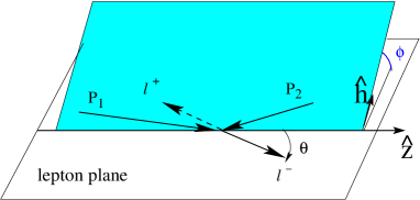
Figure 1: The Collins-Soper frame.

II General formalism and approximations

In a Drell-Yan process, an antilepton and a lepton with individual momenta $k_{1}$ and $k_{2}$ are produced from the collision of two hadrons with momentum $P_{i}$, mass $M_{i}$, and spin $S_{i}$, with $i=1,2$. The center-of-mass (c.m.) square energy available is $s=(P_{1}+P_{2})^{2}$ and the invariant mass of the final pair is given by the time-like momentum transfer $q^{2}\equiv M^{2}=(k_{1}+k_{2})^{2}$. If $M^{2},s\rightarrow\infty$, while keeping the ratio $0\leq\tau=M^{2}/s\leq 1$ limited, the factorized elementary mechanism proceeds through the annihilation of a parton and an antiparton with momenta $p_{1}$ and $p_{2}$, respectively, into a virtual photon with time-like momentum $q^{2}$. If $P_{1}^{+}$ and $P_{2}^{-}$ are the dominant light-cone components of hadron momenta in this regime, then the partons are approximately collinear with the parent hadrons and carry the light-cone momentum fractions $0\leq x_{1}=p_{1}^{+}/P_{1}^{+},\;x_{2}=p_{2}^{-}/P_{2}^{-}\leq 1$, with $q^{+}=p_{1}^{+},\;q^{-}=p_{2}^{-}$ by momentum conservation Boer (1999). The transverse components ${\bm{p}}_{i{\scriptscriptstyle T}}$ of $p_{i}$ with respect to the direction defined by ${\bm{P}}_{i}(i=1,2)$, are constrained again by the momentum conservation ${\bm{q}}_{\scriptscriptstyle T}={\bm{p}}_{1{\scriptscriptstyle T}}+{\bm{p}}_{2{\scriptscriptstyle T}}$, where ${\bm{q}}_{\scriptscriptstyle T}$ is the transverse momentum of the final lepton pair. If ${\bm{q}}_{\scriptscriptstyle T}\neq 0$ the annihilation direction is not known. Hence, it is convenient to select the socalled Collins-Soper frame Collins and Soper (1977) described in Fig. 1. The final lepton pair is detected in the solid angle $(\theta,\phi)$, where, in particular, $\phi$ (and all other azimuthal angles) is measured in a plane perpendicular to the indicated lepton plane but containing $\hat{\bm{h}}={\bm{q}}_{\scriptscriptstyle T}/|{\bm{q}}_{\scriptscriptstyle T}|$.

By neglecting terms $\sim 1/M^{2}$, with $M$ the largest mass of the initial hadrons, the expression of the leading-twist differential cross section for the $H_{1}H_{2}^{\uparrow}\to l^{+}l^{-}X$ process can be written as Boer (1999)

$$\frac{d\sigma}{d\Omega dx_{1}dx_{2}d{\bm{q}}_{\scriptscriptstyle T}} = \frac{d\sigma^{o}}{d\Omega dx_{1}dx_{2}d{\bm{q}}_{\scriptscriptstyle T}}+\frac{d\Delta\sigma^{\uparrow}}{d\Omega dx_{1}dx_{2}d{\bm{q}}_{\scriptscriptstyle T}}$$ (1)

$$= \frac{\alpha^{2}}{3Q^{2}}\,\sum_{q}\,e_{q}^{2}\,\Bigg{\{}A(y)\,{\cal F}\left[f_{1}^{q}(H_{1})\,f_{1}^{q}(H_{2})\right]$$

$$\mbox{\hskip 56.9055pt}+B(y)\,\cos 2\phi\,{\cal F}\left[\left(2\hat{\bm{h}}\cdot{\bm{p}}_{1{\scriptscriptstyle T}}\,\hat{\bm{h}}\cdot{\bm{p}}_{2{\scriptscriptstyle T}}-{\bm{p}}_{1{\scriptscriptstyle T}}\cdot{\bm{p}}_{2{\scriptscriptstyle T}}\right)\,\frac{h_{1}^{\perp\,q}(H_{1})\,h_{1}^{\perp\,q}(H_{2})}{M_{1}\,M_{2}}\,\right]\Bigg{\}}$$

$$+\frac{\alpha^{2}}{3Q^{2}}\,|{\bm{S}}_{2{\scriptscriptstyle T}}|\,\sum_{q}\,e_{q}^{2}\,\Bigg{\{}A(y)\,\sin(\phi-\phi_{S_{2}})\,{\cal F}\left[\hat{\bm{h}}\cdot{\bm{p}}_{2{\scriptscriptstyle T}}\,\frac{f_{1}^{q}(H_{1})\,f_{1{\scriptscriptstyle T}}^{\perp\,q}(H_{2}^{\uparrow})}{M_{2}}\right]$$

$$\mbox{\hskip 85.35826pt}-B(y)\,\sin(\phi+\phi_{S_{2}})\,{\cal F}\left[\hat{\bm{h}}\cdot{\bm{p}}_{1{\scriptscriptstyle T}}\,\frac{h_{1}^{\perp\,q}(H_{1})\,h_{1}^{q}(H_{2}^{\uparrow})}{M_{1}}\right]\,\Bigg{\}}\;,$$

where $\alpha$ is the fine structure constant, $d\Omega=\sin\theta d\theta d\phi$, $e_{q}$ is the charge of the parton with flavor $q$, $\phi_{S_{2}}$ is the azimuthal angle of the transverse polarization vector of the hadron $H_{2}^{\uparrow}$, and

$$A(y)=\left(\frac{1}{2}-y+y^{2}\right)\,\stackrel{{\scriptstyle\mbox{cm}}}{{=}}\,\frac{1}{4}\left(1+\cos^{2}\theta\right) \mbox{\hskip 56.9055pt}B(y)=y(1-y)\,\stackrel{{\scriptstyle\mbox{cm}}}{{=}}\,\frac{1}{4}\,\sin^{2}\theta\;.$$ (2)

The TMD functions $f_{1}^{q}(H),\,h_{1}^{\perp\,q}(H)$, describe the distributions of unpolarized and transversely polarized partons in an unpolarized hadron $H$, respectively, while $f_{1{\scriptscriptstyle T}}^{\perp\,q}(H^{\uparrow})$ and $h_{1}^{q}(H^{\uparrow})$ have a similar interpretation but for transversely polarized hadrons $H^{\uparrow}$. The convolutions are defined as

$${\cal F}\left[\mbox{TMD}_{1}^{q}(H_{1})\,\mbox{TMD}_{2}^{q}(H_{2}^{(\uparrow)})\right] \equiv \int d{\bm{p}}_{1{\scriptscriptstyle T}}d{\bm{p}}_{2{\scriptscriptstyle T}}\,\delta\left({\bm{p}}_{1{\scriptscriptstyle T}}+{\bm{p}}_{2{\scriptscriptstyle T}}-{\bm{q}}_{\scriptscriptstyle T}\right)$$ (3)

$$\mbox{\hskip 56.9055pt}\times\left[\mbox{TMD}_{1}(x_{1},{\bm{p}}_{1{\scriptscriptstyle T}};\bar{q}/H_{1})\,\mbox{TMD}_{2}(x_{2},{\bm{p}}_{2{\scriptscriptstyle T}};q/H_{2}^{(\uparrow)})+(q\leftrightarrow\bar{q})\right]\;.$$

The Monte Carlo events have been generated by the following cross section Bianconi and Radici (2005a):

$$\frac{d\sigma}{d\Omega dx_{1}dx_{2}d{\bm{q}}_{\scriptscriptstyle T}}=K\,\frac{1}{s}\,|{\cal T}({\bm{q}}_{\scriptscriptstyle T},x_{1},x_{2},M)|^{2}\,\sum_{i=1}^{4}\,c_{i}({\bm{q}}_{\scriptscriptstyle T},x_{1},x_{2})\,S_{i}(\theta,\phi,\phi_{{}_{S_{2}}})\;,$$ (4)

where the event distribution is driven by the elementary unpolarized annihilation, whose transition amplitude ${\cal T}$ has been highlighted. In Eq. (1), we assume a factorized transverse-momentum dependence in each TMD such as to break the convolution ${\cal F}$, leading to

$$|{\cal T}|^{2}\approx A(q_{\scriptscriptstyle T},x_{1},x_{2},M)\,F(x_{1},x_{2})\;,$$ (5)

where $q_{\scriptscriptstyle T}\equiv|{\bm{q}}_{\scriptscriptstyle T}|$. The function $A$ is parametrized and normalized as in Ref. Conway et al. (1989), where high-energy Drell-Yan $\pi-p$ collisions were considered. The average transverse momentum turns out to be $\langle q_{\scriptscriptstyle T}\rangle>1$ GeV/$c$ (see also the more recent Ref. Towell et al. (2001)), which effectively reproduces the influence of sizable QCD corrections beyond the parton model picture of Eq. (1). It is well known Altarelli et al. (1979) that such corrections induce also large $K$ factors and an $M$ scale dependence in parton distributions, determining their evolution. As in our previous works Bianconi and Radici (2005a, 2006a, b, 2006b), we conventionally assume in Eq. (4) that $K=2.5$, but we stress that in a single-spin asymmetry the corrections to the cross sections in the numerator and in the denominator should compensate each other, as it turns out to actually happen at RHIC c.m. square energies Martin et al. (1998). Since the range of $M$ values here explored is close to the one of Ref. Conway et al. (1989), where the parametrization of $A,F,$ and $c_{i}$ in Eq. (4), was deduced assuming $M$-independent parton distributions, we keep our same previous approach Bianconi and Radici (2005a, 2006a, b, 2006b) and use

$$F(x_{1},x_{2})=\frac{\alpha^{2}}{12Q^{2}}\,\sum_{q}\,e_{q}^{2}\,f_{1}^{q}(x_{1};\bar{q}/H_{1})\,f_{1}^{q}(x_{2};q/H_{2})+(\bar{q}\leftrightarrow q)\;,$$ (6)

where the unpolarized distribution $f_{1}^{q}(x)$ for various flavors $q=u,d,s,$ is taken again from Ref. Conway et al. (1989).

The whole solid angle $(\theta,\phi)$ of the final lepton pair in the Collins-Soper frame is randomly distributed in each variable. The explicit form for sorting it in the Monte-Carlo is Bianconi and Radici (2005a, 2006a, 2006b)

$$\sum_{i=1}^{4}\,c_{i}(q_{\scriptscriptstyle T},x_{1},x_{2})\,S_{i}(\theta,\phi,\phi_{S_{2}}) = (1+\cos^{2}\theta)$$ (7)

$$+\frac{\nu(q_{\scriptscriptstyle T},x_{1},x_{2})}{2}\,\sin^{2}\theta\,\cos 2\phi$$

$$+|{\bm{S}}_{2{\scriptscriptstyle T}}|\,c_{Siv}(q_{\scriptscriptstyle T},x_{1},x_{2})\,(1+\cos^{2}\theta)\,\sin(\phi-\phi_{S_{2}})$$

$$+|{\bm{S}}_{2{\scriptscriptstyle T}}|\,c_{BM}(q_{\scriptscriptstyle T},x_{1},x_{2})\,\sin^{2}\theta\,\sin(\phi+\phi_{S_{2}})\;.$$

If quarks were massless, the virtual photon would be only transversely polarized and the angular dependence would be described by the functions $c_{1}=1$ and $S_{1}=1+\cos^{2}\theta$. Violations of such azimuthal symmetry induced by the function $c_{2}\equiv\textstyle{\frac{\nu}{2}}$ are due to the longitudinal polarization of the virtual photon and to the fact that quarks have an intrinsic transverse momentum distribution, leading to the explicit dependence of $\nu$ upon $q_{\scriptscriptstyle T}$ and to the violation of the socalled Lam-Tung sum rule Falciano et al. (1986); Guanziroli et al. (1988); Conway et al. (1989). QCD corrections influence $\nu$, which in principle depends also on $M^{2}$ Conway et al. (1989). Azimuthal $\cos 2\phi$ asymmetries were simulated in Ref. Bianconi and Radici (2005a) using the simple parametrization of Ref. Boer (1999) and testing it against the previous measurement of Ref. Falciano et al. (1986); Guanziroli et al. (1988); Conway et al. (1989).

The next term in Eq. (7) describes the Sivers effect Sivers (1990):

$$c_{3}\equiv c_{Siv}(q_{\scriptscriptstyle T},x_{1},x_{2})=\frac{\sum_{q}\,e_{q}^{2}\,{\cal F}\left[\hat{\bm{h}}\cdot{\bm{p}}_{2{\scriptscriptstyle T}}\,\displaystyle{\frac{f_{1}^{q}(x_{1},{\bm{p}}_{1{\scriptscriptstyle T}})\,f_{1T}^{\perp\,q}(x_{2},{\bm{p}}_{2{\scriptscriptstyle T}})}{M_{2}}}\right]}{\sum_{q}\,e_{q}^{2}\,{\cal F}\left[f_{1}^{q}(x_{1},{\bm{p}}_{1{\scriptscriptstyle T}})\,f_{1}^{q}(x_{2},{\bm{p}}_{2{\scriptscriptstyle T}})\right]}\;,$$ (8)

while the last one contains the asymmetry induced by the socalled Boer-Mulders effect Boer (1999):

$$c_{4}\equiv c_{BM}(q_{\scriptscriptstyle T},x_{1},x_{2})=-\frac{\sum_{q}\,e_{q}^{2}\,{\cal F}\left[\hat{\bm{h}}\cdot{\bm{p}}_{1{\scriptscriptstyle T}}\,\displaystyle{\frac{h_{1}^{\perp\,q}(x_{1},{\bm{p}}_{1{\scriptscriptstyle T}})\,h_{1}^{q}(x_{2},{\bm{p}}_{2{\scriptscriptstyle T}})}{M_{1}}}\right]}{\sum_{q}\,e_{q}^{2}\,{\cal F}\left[f_{1}^{q}(x_{1},{\bm{p}}_{1{\scriptscriptstyle T}})\,f_{1}^{q}(x_{2},{\bm{p}}_{2{\scriptscriptstyle T}})\right]}\;.$$ (9)

In the following, we will consider the asymmetry generated only by $c_{Siv}$ in Eq. (8), because there is a sufficient amount of available data to support the construction of realistic parametrizations for the Sivers function $f_{1T}^{\perp}$. However, our arguments can be easily generalized also to the Boer-Mulders $c_{BM}$ term. We will come back on the $\nu$ coefficient at the end of next Section.

For sake of consistency, the denominator of Eq. (8) is approximated by the same $|{\cal T}|^{2}$ of Eq. (5). As for the numerator, we first simulate the Sivers effect using the parametrization of Ref. Anselmino et al. (2005),

$$f_{1T}^{\perp\,q}(x,{\bm{p}}_{\scriptscriptstyle T}) = -2\,N_{q}\,\frac{(a_{q}+b_{q})^{a_{q}+b_{q}}}{a_{q}^{a_{q}}\,b_{q}^{b_{q}}}\,x^{a_{q}}\,(1-x)^{b_{q}}\,\frac{M_{2}M_{0}}{{\bm{p}}_{\scriptscriptstyle T}^{2}+M_{0}^{2}}\,f_{1}^{q}(x,{\bm{p}}_{\scriptscriptstyle T})$$ (10)

$$= -2\,N_{q}\,\frac{1}{\pi\,\langle p_{\scriptscriptstyle T}^{2}\rangle}\,\frac{(a_{q}+b_{q})^{a_{q}+b_{q}}}{a_{q}^{a_{q}}\,b_{q}^{b_{q}}}\,x^{a_{q}}\,(1-x)^{b_{q}}\,\frac{M_{2}M_{0}}{{\bm{p}}_{\scriptscriptstyle T}^{2}+M_{0}^{2}}\,e^{-p_{\scriptscriptstyle T}^{2}/\langle p_{\scriptscriptstyle T}^{2}\rangle}\,f_{1}^{q}(x)\;,$$

where $M_{2}$ is the mass of the polarized proton, $p_{\scriptscriptstyle T}\equiv|{\bm{p}}_{\scriptscriptstyle T}|$, and $\langle p_{\scriptscriptstyle T}^{2}\rangle=0.25$ (GeV/$c$)² is deduced by assuming a Gaussian ansatz for the ${\bm{p}}_{\scriptscriptstyle T}$ dependence of $f_{1}$ in order to reproduce the azimuthal angular dependence of the SIDIS unpolarized cross section (Cahn effect). Flavor-dependent normalization and parameters in the $x$ dependence are fitted to SIDIS SSA data using only the two flavors $q=u,d$ and neglecting the (small) contribution of antiquarks (see Refs. Anselmino et al. (2005); Bianconi and Radici (2006b)).

Following Ref. Boer (1999) and including a sign change of $f_{1T}^{\perp}$ when plugging it in the Drell-Yan cross section Collins (2002), we get

$$c_{Siv}^{A} \approx \frac{4M_{0}\,q_{\scriptscriptstyle T}}{q_{\scriptscriptstyle T}^{2}+4M_{0}^{2}}\,\frac{\sum_{q}\,e_{q}^{2}\,N_{q}\,\displaystyle{\frac{(\alpha_{q}+\beta_{q})^{\alpha_{q}+\beta_{q}}}{\alpha_{q}^{\alpha_{q}}\,\beta_{q}^{\beta_{q}}}}\,\bar{f}_{1}^{q}(x_{1})\,x_{2}^{\alpha_{q}}\,(1-x_{2})^{\beta_{q}}\,f_{1}^{q}(x_{2})}{\sum_{q}\,e_{q}^{2}\,\bar{f}_{1}^{q}(x_{1})\,f_{1}^{q}(x_{2})+(1\leftrightarrow 2)}$$ (11)

$$\equiv N_{A}(q_{\scriptscriptstyle T})\,\frac{e_{u}^{2}\,\bar{u}(x_{1})\,u_{Siv}^{A}(x_{2})+e_{d}^{2}\,\bar{d}(x_{1})\,d_{Siv}^{A}(x_{2})}{\left[e_{u}^{2}\,\bar{u}(x_{1})\,u(x_{2})+e_{d}^{2}\,\bar{d}(x_{1})\,d(x_{2})+e_{s}^{2}\,\bar{s}(x_{1})\,s(x_{2})\right]+(1\leftrightarrow 2)}\;,$$

where, for brevity, $u_{Siv}^{A}(x)$ represents the contribution of flavor $u$ to the $x$ dependence of the Sivers function parametrized as in Eq. (10) (and similarly for flavor $d$).

As an alternative choice, we adopt the new parametrization described in Ref. Bianconi and Radici (2006a, b). It is inspired to the one of Ref. Vogelsang and Yuan (2005), whose $x$ dependence is retained but a different flavor-dependent normalization and an explicit ${\bm{p}}_{\scriptscriptstyle T}$ dependence are introduced. The latter is bound to the shape of the recent RHIC data on $pp^{\uparrow}\to\pi X$ at $\sqrt{s}=200$ GeV Adler et al. (2005), where large persisting asymmetries are found that could be partly due to the leading-twist Sivers mechanism. The expression adopted is

$$f_{1T}^{\perp\,q}(x,{\bm{p}}_{\scriptscriptstyle T}) = N_{q}\,x\,(1-x)\,\frac{M_{2}p_{0}^{2}p_{\scriptscriptstyle T}}{(p_{\scriptscriptstyle T}^{2}+\frac{p_{0}^{2}}{4})^{2}}\,f_{1}^{q}(x,{\bm{p}}_{\scriptscriptstyle T})$$ (12)

$$= N_{q}\,x\,(1-x)\,\frac{M_{2}p_{0}^{2}p_{\scriptscriptstyle T}}{(p_{\scriptscriptstyle T}^{2}+\frac{p_{0}^{2}}{4})^{2}}\,\frac{1}{\pi\,\langle p_{\scriptscriptstyle T}^{2}\rangle}\,e^{-p_{\scriptscriptstyle T}^{2}/\langle p_{\scriptscriptstyle T}^{2}\rangle}\,f_{1}^{q}(x)\;,$$

where $p_{0}=2$ GeV/$c$, and $N_{u}=-N_{d}=0.7$. The sign, positive for $u$ quarks and negative for the $d$ ones, already takes into account the predicted sign change of $f_{1{\scriptscriptstyle T}}^{\perp}$ from Drell-Yan to SIDIS Collins (2002).

Along the same previous lines, we get

$$c_{Siv}^{B} \approx \left(\frac{2\,p_{0}\,q_{\scriptscriptstyle T}}{q_{\scriptscriptstyle T}^{2}+p_{0}^{2}}\right)^{2}\,\frac{\sum_{q}\,e_{q}^{2}\,N_{q}\,\bar{f}_{1}^{q}(x_{1})\,x_{2}\,(1-x_{2})\,f_{1}^{q}(x_{2})}{\sum_{q}\,e_{q}^{2}\,\bar{f}_{1}^{q}(x_{1})\,f_{1}^{q}(x_{2})+(1\leftrightarrow 2)}$$ (13)

$$\equiv N_{B}(q_{\scriptscriptstyle T})\,\frac{e_{u}^{2}\,\bar{u}(x_{1})\,u_{Siv}^{B}(x_{2})+e_{d}^{2}\,\bar{d}(x_{1})\,d_{Siv}^{B}(x_{2})}{\left[e_{u}^{2}\,\bar{u}(x_{1})\,u(x_{2})+e_{d}^{2}\,\bar{d}(x_{1})\,d(x_{2})+e_{s}^{2}\,\bar{s}(x_{1})\,s(x_{2})\right]+(1\leftrightarrow 2)}\;,$$

where now $u_{Siv}^{B}(x)$ indicates the contribution of flavor $u$ to the $x$ dependence of the Sivers function parametrized as in Eq. (12).

In the following, we will refer to ”framework I” as to the $(1+\cos^{2}\theta)\,\sin(\phi-\phi_{S_{2}})$ angular asymmetry generated in Eq. (1) by the coefficients (11) or (13).

The coefficients $c_{Siv}^{A}$ and $c_{Siv}^{B}$ can be further approximated with a procedure that here we will conventionally indicate as ”framework II”. Again, following the lines described in Refs. Bianconi and Radici (2006a, b) we obtain

$$c_{Siv}^{A} = N_{A}(q_{\scriptscriptstyle T})\,\frac{e_{u}^{2}\,\bar{u}(x_{1})\,u_{Siv}^{A}(x_{2})+e_{d}^{2}\,\bar{d}(x_{1})\,d_{Siv}^{A}(x_{2})}{\left[e_{u}^{2}\,\bar{u}(x_{1})\,u(x_{2})+e_{d}^{2}\,\bar{d}(x_{1})\,d(x_{2})+e_{s}^{2}\,\bar{s}(x_{1})\,s(x_{2})\right]+(1\leftrightarrow 2)}$$ (14)

$$\approx N_{A}(q_{\scriptscriptstyle T})\,\left[n_{u}^{A}\,\frac{u_{Siv}^{A}(x_{2})}{u(x_{2})}+n_{d}^{A}\,\frac{d_{Siv}^{A}(x_{2})}{d(x_{2})}\right]\;,$$

and

$$c_{Siv}^{B} = N_{B}(q_{\scriptscriptstyle T})\,\frac{e_{u}^{2}\,\bar{u}(x_{1})\,u_{Siv}^{B}(x_{2})+e_{d}^{2}\,\bar{d}(x_{1})\,d_{Siv}^{B}(x_{2})}{\left[e_{u}^{2}\,\bar{u}(x_{1})\,u(x_{2})+e_{d}^{2}\,\bar{d}(x_{1})\,d(x_{2})+e_{s}^{2}\,\bar{s}(x_{1})\,s(x_{2})\right]+(1\leftrightarrow 2)}$$ (15)

$$\approx N_{B}(q_{\scriptscriptstyle T})\,\left[n_{u}^{B}\,\frac{u_{Siv}^{B}(x_{2})}{u(x_{2})}+n_{d}^{B}\,\frac{d_{Siv}^{B}(x_{2})}{d(x_{2})}\right]\;.$$

The coefficients $n_{q}$ ($q=u,d$) include the contribution of the quark charge, of the normalization of the parton distributions, as well as of the statistical weight of the considered flavor. In fact, the approximation is based on the idea that each term in both flavor sums in the numerator and denominator can be replaced by a ”flavor-averaged” one, and the resulting simplified ratio is then properly weighted. For example, in a $\bar{p}p^{\uparrow}$ collision where only valence contributions are considered and the $u(x)$ distribution in $p$ is normalized to 2 (and similarly for the $\bar{u}$ one in $\bar{p}$), we easily get a statistical ratio 16:1 of the $\bar{u}u^{\uparrow}$ annihilations over the $\bar{d}d^{\uparrow}$ ones, such that $n_{u}=16/17,\,n_{d}=1/17$.

The underlying idea in ”framework II” is that there is no strong flavor dependence in the sums appearing in Eqs. (11) and (13), and that it is possible to neglect the contribution from sea (anti)quarks. The latter feature is included by construction in the parametrizations of the Sivers functions, in agreement with the common belief about the behaviour of SSA at low $x$. It is far less obvious that the approximation can be safely carried on also in the denominator of the asymmetries $c_{Siv}^{A/B}$, where the unpolarized distributions $f_{1}$ are involved. In the next Section, we will numerically simulate $\pi^{\pm}p^{\uparrow}$ and $\bar{p}p^{\uparrow}$ Drell-Yan collisions to explore the effect of neglecting such terms.

III Monte Carlo simulation and discussion of results

In this Section, we present results for the Monte Carlo simulation of the Sivers effect in several Drell-Yan events using transversely polarized proton targets by adopting either ”framework I” or ”framework II”, as they are described in the previous Section. The goal is to explore the sensitivity of the results when the contribution of unpolarized sea (anti)quarks is neglected in the denominator of the SSA, as it is usually done when parametrizing the Sivers function from experimental data.

In the Monte Carlo, events are simulated by the cross section (4) with ”framework II”, namely using Eqs. (14) or (15) according to the input parametrization selected for the Sivers function Anselmino et al. (2005); Bianconi and Radici (2006a, b); the unpolarized parton distributions are parametrized following Ref. Conway et al. (1989), as explained in the previous Section when discussing Eqs. (5) and (6). Events for the Sivers effect are then rejected/accepted by constructing the spin asymmetry $A^{\prime}=(U^{\prime}-D^{\prime})/(U^{\prime}+D^{\prime})$, where $U^{\prime}$ ($D^{\prime}$) represents events with positive (negative) values of $\sin(\phi-\phi_{S_{2}})$ in Eq. (7). Similarly, the spin asymmetry $A=(U-D)/(U+D)$ is obtained by rejecting/accepting events using the ”framework I”, namely using Eqs. (11) or (13), for positive ($U$) or negative ($D$) values of $\sin(\phi-\phi_{S_{2}})$. Data are accumulated only in the $x_{2}$ bins of the polarized proton, i.e. they are summed over in the $x_{1}$ bins for the hadronic beam, in the transverse momentum $q_{\scriptscriptstyle T}$ of the lepton pair and in their zenithal orientation $\theta$. In the following, plots will compare $A$ and $A^{\prime}$ for different Drell-Yan processes and kinematical conditions, showing only the positive values of the asymmetries (the negative ones look equally distributed in a symmetric way).

All events refer to collisions at $s=100$ GeV², which can be explored either at GSI in the socalled collider mode, or at COMPASS with fixed targets. The lepton pair invariant mass is constrained in the ranges $4<M<6$ GeV and $1.5<M<2.5$ GeV in order to avoid overlaps with the resonances of the $\bar{c}c$ and $\bar{b}b$ quarkonium systems, while exploring at the same time different $\langle x_{2}\rangle$ regions which stress the role of sea (anti)quarks. The transverse momentum of the lepton pair is constrained in the range $1<q_{\scriptscriptstyle T}<3$ GeV/$c$ in order to avoid a strong dilution of the SSA because of the rapid decrease of the distributions (10) and (12) at larger $q_{\scriptscriptstyle T}$. Moreover, the resulting $\langle q_{\scriptscriptstyle T}\rangle\sim 1.8$ GeV/$c$ is in fair agreement with the one experimentally explored at RHIC Adler et al. (2005).

Figure 2: Scatter plot for single-spin asymmetries $A$ and $A^{\prime}$, calculated with ”framework I” and ”framework II” (see text), produced by $7\,000$ events of the Sivers effect in the $\bar{p}p^{\uparrow}\to\mu^{+}\mu^{-}X$ process with muon invariant mass $1.5<M<2.5$ GeV and transverse momentum $1<q_{\scriptscriptstyle T}<3$ GeV/$c$, where only (polarized) valence contributions are considered and $u_{Siv}(x)\equiv u(x),\,d_{Siv}(x)\equiv d(x)$.

The considered Drell-Yan collisions involve transversely polarized protons and different hadronic probes: antiprotons ($\bar{p}$) and pions ($\pi^{-}$ and $\pi^{+}$). The statistical sample is made of $7\,000$ events except for the $\pi^{+}$ probe, where we have used $20\,000$ events because the Monte Carlo indicates that the cross section involving $\pi^{+}$ is statistically disfavoured by approximately a factor 1/4 Bianconi (2005).

As a sort of ”warm up”, we first consider oversimplified cases where the simulated comparison between $A$ and $A^{\prime}$ can be confronted with a priori known results. In Fig. 2, we show the scatter plot of $A$ versus $A^{\prime}$ for the $\bar{p}p^{\uparrow}\to\mu^{+}\mu^{-}X$ process with $1.5<M<2.5$ GeV where only (polarized) valence contributions are considered and $u_{Siv}(x)\equiv u(x),\,d_{Siv}(x)\equiv d(x)$. From Eq. (14), it is evident that both ”framework I” and ”framework II” must give the same result, namely

$$c_{Siv}^{I} \propto \frac{e_{u}^{2}\,\bar{u}(x_{1})\,u_{Siv}(x_{2})+e_{d}^{2}\,\bar{d}(x_{1})\,d_{Siv}(x_{2})}{e_{u}^{2}\,\bar{u}(x_{1})\,u(x_{2})+e_{d}^{2}\,\bar{d}(x_{1})\,d(x_{2})}\equiv 1$$

$$c_{Siv}^{II} \propto \left[n_{u}\,\frac{u_{Siv}(x_{2})}{u(x_{2})}+n_{d}\,\frac{d_{Siv}(x_{2})}{d(x_{2})}\right]\equiv n_{u}+n_{d}=1\;,$$ (16)

because any flavor dependence has been switched off and for ”framework I” the asymmetry $A$ is not diluted by the contribution of unpolarized sea (anti)quarks showing up in the denominator of the first equality in Eq. (14) itself (the socalled ”sea dilution effect”). From the figure we get the consistent picture that the SSA calculated with the two methods are statistically equal. We have checked that the same result holds also for $\pi^{\pm}$ probes, as it is obvious.

Figure 3: Scatter plot in the same conditions as previous figure, but for the $\pi^{-}p^{\uparrow}\to\mu^{+}\mu^{-}X$ process with muon invariant mass $4<M<6$ GeV and including the contribution of unpolarized sea (anti)quarks.

In Fig. 3, the scatter plot is shown for the $\pi^{-}p^{\uparrow}\to\mu^{+}\mu^{-}X$ process with $4<M<6$ GeV where still $u_{Siv}(x)\equiv u(x),\,d_{Siv}(x)\equiv d(x)$, but the contribution of the unpolarized sea (anti)quarks is included. Therefore, we have

$$c_{Siv}^{I} \propto \frac{e_{u}^{2}\,\bar{u}(x_{1})\,u_{Siv}(x_{2})+e_{d}^{2}\,\bar{d}(x_{1})\,d_{Siv}(x_{2})}{\left[e_{u}^{2}\,\bar{u}(x_{1})\,u(x_{2})+e_{d}^{2}\,\bar{d}(x_{1})\,d(x_{2})+e_{s}^{2}\,\bar{s}(x_{1})\,s(x_{2})\right]+(1\leftrightarrow 2)}$$ (17)

$$\equiv \frac{e_{u}^{2}\,\bar{u}(x_{1})\,u(x_{2})+e_{d}^{2}\,\bar{d}(x_{1})\,d(x_{2})}{\left[e_{u}^{2}\,\bar{u}(x_{1})\,u(x_{2})+e_{d}^{2}\,\bar{d}(x_{1})\,d(x_{2})+e_{s}^{2}\,\bar{s}(x_{1})\,s(x_{2})\right]+(1\leftrightarrow 2)}$$

$$= \left[1+\frac{e_{u}^{2}\,u(x_{1})\,\bar{u}(x_{2})+e_{d}^{2}\,d(x_{1})\,\bar{d}(x_{2})+e_{s}^{2}\,\bar{s}(x_{1})\,s(x_{2})+e_{s}^{2}\,s(x_{1})\,\bar{s}(x_{2})}{e_{u}^{2}\,\bar{u}(x_{1})\,u(x_{2})+e_{d}^{2}\,\bar{d}(x_{1})\,d(x_{2})}\right]^{-1}<1$$

$$c_{Siv}^{II} \propto \left[n_{u}\,\frac{u_{Siv}(x_{2})}{u(x_{2})}+n_{d}\,\frac{d_{Siv}(x_{2})}{d(x_{2})}\right]\equiv n_{u}+n_{d}=1\;.$$ (18)

Evidently, the difference between the two approaches stems from the unpolarized sea-(anti)quark contribution, both in the numerator and in the denominator of $c_{Siv}^{I}$, and it is responsible for the (limited) spreading of some events in the scatter plot.

Figure 4: Scatter plot in the same conditions as previous figure, but for muon invariant mass $1.5<M<2.5$ GeV.

In Fig. 4, the same situation is shown for muon invariant masses $1.5<M<2.5$ GeV. At the given $s=100$ GeV², lower $M$ implies testing lower $x_{2}$ values, typically below 0.05-0.1, where sea effects start dominating over the valence contribution. Consequently, the ”sea dilution effect” becomes stronger and the marked difference between ”framework I” and ”framework II” produces the scattering of events observed in the plot. In summary, the two approaches become equivalent when the polarized distributions weakly depend on flavor (or, equivalently, one flavor dominates the flavor sum in the numerator of the SSA), and the contribution of sea (anti)quarks becomes negligible, i.e. for not too low $\langle x\rangle$ and, consequently, $M$ (assuming that also transversely polarized sea (anti)quarks can be neglected, as well).

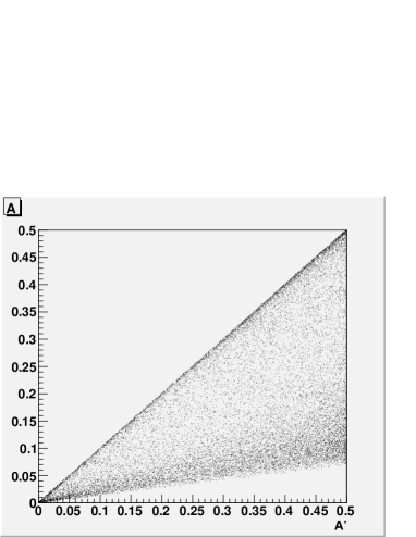
Figure 5: Scatter plot in the same conditions as previous figure, but for the $\pi^{+}p^{\uparrow}\to\mu^{+}\mu^{-}X$ process.

In Fig. 5, the same kinematical situation of the previous figure is considered for $\pi^{+}$ probes. Equations (17) and (18) formally still hold. However, while the latter remains obviously unchanged, the former can be usefully compared in the two cases by adopting some simple approximations. In fact, if we neglect the product of two sea-quark distributions and we assume isospin symmetry among the valence distributions of the $\pi^{\pm}$ probes (i.e., $u_{\pi^{+}}(x)=\bar{u}_{\pi^{-}}(x)=u_{\pi}(x)\equiv u(\pi)$ and $\bar{d}_{\pi^{+}}(x)=d_{\pi^{-}}(x)=d_{\pi}(x)\equiv d(\pi)$), we get for the $\pi^{-}$ probe

$$c_{Siv\,\pi^{-}}^{I}\propto\left[1+\frac{d(\pi)\,\bar{d}(p)}{u(\pi)\,u(p)+\bar{d}(\pi^{-})\,d(p)}\right]^{-1}\;,$$ (19)

and for the $\pi^{+}$ probe

$$c_{Siv\,\pi^{+}}^{I}\propto\left[1+\frac{4u(\pi)\,\bar{u}(p)}{d(\pi)\,d(p)+8\bar{u}(\pi^{+})\,u(p)}\right]^{-1}\;.$$ (20)

For sake of simplicity, we further assume the flavor independence of the sea contributions, namely $\bar{d}(\pi^{-})=\bar{u}(\pi^{+})\equiv q_{sea}(\pi)\ll u(\pi),\,d(\pi)$ and $\bar{u}(p)=\bar{d}(p)\equiv q_{sea}(p)\ll u(p),\,d(p)$. It is also reasonable to consider $u(\pi)>d(\pi)$ and $u(p)>d(p)$. From these inequalities it follows that

$$\frac{d(\pi)\,q_{sea}(p)}{u(\pi)\,u(p)+q_{sea}(\pi)\,d(p)}\,<\,\frac{4u(\pi)\,q_{sea}(p)}{d(\pi)\,d(p)+8q_{sea}(\pi)\,u(p)}\;,$$ (21)

namely $c_{Siv\,\pi^{-}}^{I}$ is closer to $c_{Siv}^{II}=1$ than $c_{Siv\,\pi^{+}}^{I}$. This fact is responsible for the plot in Fig. 5 showing much more scattered events than in Fig. 4. Given the lowest $M$ range here explored, the situation displayed in Fig. 5 represents a sort of ideal upper limit to the potential discrepancy between the two methods for calculating the Drell-Yan SSA.

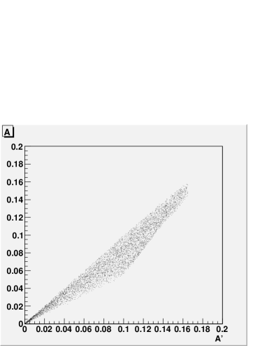
Figure 6: Scatter plot in the same conditions as Fig. 4, but using the parametrization of the Sivers function from Ref. Anselmino et al. (2005).

We now turn to the comparison between ”framework I” and ”framework II” with realistic parametrizations of the Sivers function and including the ”sea dilution effect”. In Fig. 6, the scatter plot of $A$ versus $A^{\prime}$ is shown for the $\pi^{-}p^{\uparrow}\to\mu^{+}\mu^{-}X$ process with $1.5<M<2.5$ GeV using the Sivers function of Ref. Anselmino et al. (2005), i.e. using $c_{Siv}^{A}$ from Eqs. (11) and (14). The discrepancy is not large, if we consider the potentially dangerous low $M$ range.

Figure 7: Scatter plot in the same conditions as previous figure, but using the parametrization of the Sivers function from Ref. Bianconi and Radici (2006a, b) and for muon invariant mass $4<M<6$ GeV.

In Fig. 7, the same situation of the previous case is simulated at $4<M<6$ GeV using the Sivers function from Ref. Bianconi and Radici (2006a, b). Here, the agreement between the two methods is much more evident also because the higher $M$ range considered corresponds to a safer valence domain in $x_{2}$, approximately around 0.2-0.4.

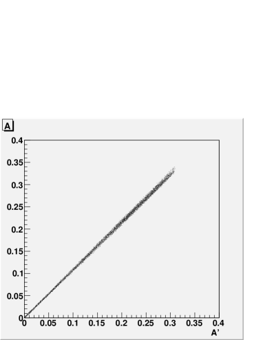
Figure 8: Scatter plot in the same conditions as previous figure, but for the $\bar{p}p^{\uparrow}\to\mu^{+}\mu^{-}X$ process.

Next, in Fig. 8 we reconsider the situation of the previous figure but for the $\bar{p}p^{\uparrow}\to\mu^{+}\mu^{-}X$ process. At the level of leading valence contributions to the asymmetry, the $\pi^{-}p^{\uparrow}$ and the $\bar{p}p^{\uparrow}$ collisions are equivalent because they are both dominated by the $\bar{u}u^{\uparrow}$ annihilation. Hence, the persisting close similarity of $A$ and $A^{\prime}$ indicates that the main origin of the discrepancy between ”framework I” and ”framework II” comes from the ”sea dilution effect”, namely from including or neglecting the contribution of unpolarized sea (anti)quarks in the denominator of the SSA.

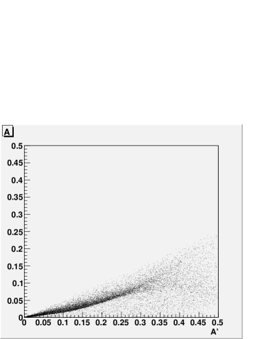
Figure 9: Scatter plot in the same conditions as Fig. 6, but for the $\pi^{+}p^{\uparrow}\to\mu^{+}\mu^{-}X$ process.

Last, in Fig. 9 we show the scatter plot of $A$ versus $A^{\prime}$ in the same conditions as in Fig. 6 but for the $\pi^{+}p^{\uparrow}\to\mu^{+}\mu^{-}X$ process. The large discrepancies confirm the findings about Eq. (21) that were displayed in Fig. 5 using a simpler naive parametrization of the Sivers function: with the $\pi^{+}$ probe the ”sea dilution effect” is emphasized and the approximations introduced in ”framework II” with Eq. (14) are somewhat not justified. The effect is also emphasized by the low $M$ range considered.

In summary, when the spin asymmetries $A$ and $A^{\prime}$ are simulated using realistic parametrizations of the Sivers function, which are all based on the dominance of the transversely polarized $u^{\uparrow}$ valence distribution in the transversely polarized $p^{\uparrow}$ parent hadron, their results are very close provided that the effect of the unpolarized sea (anti)quarks can be neglected. This condition is fulfilled by the $\pi^{-}$ and $\bar{p}$ probes at not too low muon invariant masses $M$, which correspond to the safe valence domain in $x$. In these cases, the originating schemes ”framework I” and ”framework II” can be considered equivalent.

However, the last statement can be misleading, because the realistic parametrizations of the Sivers function are obtained in the ”framework II”, namely by building the SSA by neglecting the unpolarized sea (anti)quarks. It means that any contribution from the sea, which is intrinsically contained in the experimental measurement of the asymmetry, is effectively reproduced in the parametrization, particularly in the behaviour at low $x$. For example, this ”hidden sea effect” is contained in the $\alpha_{q}$ parameter of the $x^{\alpha_{q}}$ factor in Eq. (11), which is determined from a fit of experimental SSA based on valence $q=u,d$ degrees of freedom only Anselmino et al. (2005). Hence, it can be over- or under-estimated when the related Sivers function is plugged into expressions of SSA constructed with ”framework I” or ”framework II”.

Actually, the emerging issue here is that ”framework I”, which looks more correct because it properly includes the unpolarized sea contribution in the denominator of the SSA, could produce a sort of double counting when employing a Sivers function in the numerator that is parametrized with valence quarks only. Consequently, it is not obvious that the approximations adopted in ”framework II” (and systematically used in the analysis of several Drell-Yan SSA in Refs. Bianconi and Radici (2005a, b, 2006a, 2006b)) are crude ones; rather, they look like the most appropriate framework for using the parametrized Sivers functions available in the literature. However, this last statement should be generalized with some care. In fact, the large discrepancies observed in the results obtained with ”framework I” and ”framework II” using $\pi^{+}$ probes, suggest that each physics case should be separately considered.

Finally, as anticipated in Sec. II, we reconsider the $\nu$ term in Eq. (7), which is most likely related to the violation of the Lam-Tung sum rule Falciano et al. (1986); Guanziroli et al. (1988); Conway et al. (1989). The corresponding azimuthal $\cos 2\phi$ asymmetry in the unpolarized Drell-Yan cross section was simulated in Ref. Bianconi and Radici (2005a) using the simple parametrization of Ref. Boer (1999) and testing it against the previous measurements of Refs. Falciano et al. (1986); Guanziroli et al. (1988); Conway et al. (1989). The Boer-Mulders function $h_{1}^{\perp}(x)$ was parametrized in Ref. Boer (1999) exactly in the ”framework II” but with no flavor dependence, because of few available data at that time. The latter span only the region $x>0.3$, while for $x<0.3$ the $\nu$ function was assumed to be independent from $x$. Hence, the present parametrization of $h_{1}^{\perp}$ does not effectively include any ”sea dilution effect”. The situation could be improved by either refitting the Drell-Yan data of Refs. Falciano et al. (1986); Guanziroli et al. (1988); Conway et al. (1989) using ”framework I” and an $x$-independent $\nu$ function for $x<0.3$, or using ”framework II” and introducing a specific $x^{\alpha}$ power law to extrapolate the behaviour at low $x$. Moreover, new data have been recently released for Drell-Yan muon pairs produced in high-energy proton-deuteron collisions Zhu et al. (2006), that show no evidence of a $\cos 2\phi$ asymmetry at very low $x$. In any case, the few available data do not allow yet a full flavor-dependent analysis and any conclusion is, consequently, premature.

IV Conclusions

In this paper, we performed numerical simulations of the socalled Sivers effect Sivers (1990), as it can be isolated in single spin asymmetries (SSA) of the distribution of Drell-Yan muon pairs produced from collisions of transversely polarized protons and different hadronic probes. Several measurements of such SSA are planned by experimental collaborations (RHIC at BNL, COMPASS at CERN, PANDA and PAX at GSI, and, possibly, also future experiments at JPARC). The goal is the extraction of the socalled Sivers function $f_{1{\scriptscriptstyle T}}^{\perp}$, a leading-twist parton distribution that can give direct insight into the orbital motion and the spatial distribution of hidden confined partons, with interesting connections with the problem of the proton spin sum rule and the powerful formalism of Generalized Parton Distributions Burkardt and Hwang (2004). In particular, it would be extremely important to verify the peculiar universality properties of such parton density, namely its predicted sign change with respect to the same $f_{1{\scriptscriptstyle T}}^{\perp}$ as it is parametrized to reproduce the SSA in SIDIS measurements Bianconi and Radici (2006a, b). This theorem is based on very general assumptions and it represents a formidable test of QCD universality Collins (2002).

One of the main features of the SIDIS phenomenological parametrizations is the approximation of neglecting both polarized and unpolarized nonvalence partons (see, e.g., Ref. Anselmino et al. (2005)), which actually amounts to effectively include their contribution in the fitting parameters of the valence partons for the $x$ range considered. We conventionally name this the ”hidden sea effect”. In a series of previous papers Bianconi and Radici (2005a, b, 2006a, 2006b), we performed numerical simulations of Drell-Yan SSA with transversely polarized protons using colliding protons, antiprotons, and pions, in various kinematics of interest for the planned experiments. In our Monte Carlo code, the Sivers effect was consistently simulated within the same approach, but we further conveniently made a suitable flavor average of the valence contribution which allows for a great simplification of formulae. We conventionally name this scheme as ”framework II”. Here, we consider also the socalled ”framework I”, where we release the approximation about the flavor average and we include also the unpolarized nonvalence contribution, which shows up mainly in the denominator of the SSA; as such, we conventionally refer to the ”sea dilution effect”.

We have explored the deviations of ”framework II” from the more appropriate ”framework I” in the simulation of the Sivers effect for the $Hp^{\uparrow}\to\mu^{+}\mu^{-}X$ process at $s=100$ GeV² with $H=\bar{p},\pi^{-},\pi^{+}$ and different muon invariant masses. It turns out that the two approaches become approximately equivalent when the polarized distributions weakly depend on flavor (or, equivalently, one flavor dominates the flavor sum in the numerator of the SSA), and for sufficiently high muon invariant masses (typically, $4<M<6$ GeV), which correspond to $\langle x\rangle$ in the safe valence domain where the contribution of sea (anti)quarks becomes negligible (assuming that also transversely polarized sea (anti)quarks can be neglected, as well). These conditions can be fulfilled when using the $\pi^{-}$ and $\bar{p}$ probes; on the contrary, the valence structure of $\pi^{+}$ emphasizes the role of the ”sea dilution effect” and leads to larger discrepancies.

However, we must remark that the parametrizations of the Sivers function are basically obtained using ”framework II”, since all sea (anti)quarks are neglected. Hence, the ”hidden sea effect” contained in the values of the parameters can be over- or under-estimated when the related Sivers function is plugged into expressions of SSA constructed with ”framework I” or ”framework II”. Actually, the ”framework I” appears even less appropriate, since it could lead to a double counting of the contribution of unpolarized sea (anti)quarks; in our jargon, the ”sea dilution effect” induced by the denominator of the SSA would describe the same mechanisms as the ”hidden sea effect” contained in the fitting parameters of the valence quark distributions. Correspondingly, the approximations adopted in ”framework II” (and systematically used in the analysis of Refs. Bianconi and Radici (2005a, b, 2006a, 2006b)) look like the most appropriate approach for using the parametrized Sivers functions presently available in the literature. However, this statement should be taken with some care, because there are cases like the $\pi^{+}p^{\uparrow}$ collisions where the ”framework II” largely deviates from ”framework I” in any kinematics and seems not well justified.

In our work, the Sivers effect has been used as a test case since the abundance of data allows for a flavor-dependent analysis. In principle, the arguments can be generalized to other interesting azimuthal asymmetries in Drell-Yan processes, such as the Boer-Mulders effect or the violation of the Lam-Tung sum rule. But in the former case, there are no experimental data, while in the latter the few ones available Falciano et al. (1986); Guanziroli et al. (1988); Conway et al. (1989); Zhu et al. (2006) do not permit to discriminate the contributions of each flavor and prevent from coming to definite conclusions.