Fermion Masses at intermediate $\mathop{\rm tan}\beta$: Unification of Yukawa Determinants

Abstract

In the context of the Grand Unified MSSM, we investigate the fermion mass matrices at GUT scale. We note that from the experimental mass pattern the determinants of the Yukawa matrices at this scale can be unified with good precision. Taking the unification o determinants as an hypothesis, it gives two model independent predictions that in the MSSM turns out to determine an appropriate value for the product $m_{d}m_{s}$ and $\mathop{\rm tan}\beta\simeq 7$–$10$ in the favored range. We then review a predictive model of SU(3) flavour in the context of supersymmetric SO(10) that nicely implements this mechanism, while explaining all fermion masses and mixings at 1$\sigma$ level, including neutrino data.

1 Introduction

Understanding the physics that underlies the measured pattern of fermion masses and mixings is still an open problem. While there is little clue on the way to follow, it is certain that one will need a framework beyond the Standard Model. We approach here the problem in the interesting setup of SO(10) Supersymmetric Grand Unification (SUSY GUT) [1] with an horizontal SU(3) flavour symmetry [2]. The reason for this choice is of course that all the fermions of a Standard Model family plus the right-handed neutrino fit in a basic multiplet of SO(10), the $\mathbf{16}$ representation, and that the SU(3) flavour symmetry is the largest allowed (actually U(3)) by gauge interactions. SUSY provides a one-scale unification of the gauge couplings, in addition to benefits like the stability of the (large) hierarchy, and others.

While in the low energy world both the gauge SO(10) and flavour SU(3) symmetries are broken, in this framework the Yukawa matrices are treated in an unified way, so that they will show the remnants of both these breakings.

With this in mind we approach the problem by studying the mass matrices at the Grand-Unification scale $M_{GUT}\simeq 2\cdot 10^{16}\,\mbox{GeV}$. We consider first the charged-fermions Yukawa couplings renormalized at this common scale assuming MSSM running (recalled in appendix A). We plot them in figure 1, showing also the ranges resulting from experimental uncertainties, and illustrating the three relevant cases of small, moderate and large $\mathop{\rm tan}\beta$.

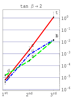
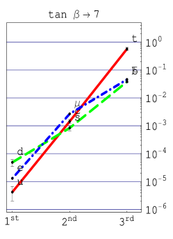
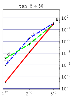
Figure 1: Yukawa couplings at GUT scale calculated from experimental charged fermions masses, assuming MSSM running and including uncertainties also from $\lambda_{t}$ renormalization. U, D, E are respectively red (continuous), green (dashed) and blue (dot-dashed).

The first observation that one can make in figure 1 is that the Yukawa couplings show clear hierarchic patterns: indeed if it were not for some deviations, the picture would be quite simple: $\lambda_{f}\sim\epsilon_{f}^{2}:\epsilon_{f}:1$, with small parameters $\epsilon_{f}$, for $f=u,d,e$. One can estimate the hierarchy parameters as $\epsilon_{u}\sim 1/500$ in the “up” sector, while in the “down” and “charged leptons” sectors the hierarchies are very similar, $\epsilon_{d,e}\simeq 1/50$, reaching the well known observation that $\epsilon_{u}\ll\epsilon_{e}\simeq\epsilon_{d}$.

About the deviations, it is evident that the “up” sector (U) has an almost exact hierarchy, while the “down” and “charged leptons” sectors (D, E) deviate sensibly. These deviations can be thought to belong mainly to the first two generations, so that the picture that emerges is the following:

$$\lambda_{u}\ :\ \lambda_{c}\ :\ \lambda_{t} \ \sim\ \ \epsilon_{u}^{2}\ \ \ \ :\ \ \ \epsilon_{u}\ \ \ :\ \ 1$$ (1)

$$\lambda_{d}\ :\ \lambda_{s}\ :\ \lambda_{b} \ \sim\ \frac{1}{A_{d}}\,\epsilon_{d}^{2}\ :\ A_{d}\,\epsilon_{d}\ :\ \ 1$$ (2)

$$\lambda_{e}\ :\ \lambda_{\mu}\ :\ \lambda_{\tau} \ \sim\ \frac{1}{A_{e}}\,\epsilon_{e}^{2}\ :\ A_{e}\,\epsilon_{e}\ :\ \ 1\,.$$ (3)

The factors $A_{e}$, $A_{d}$ that parametrize the deviations can also be estimated as $A_{e}\simeq 2.5$ and $A_{d}\simeq 0.5$.

Other noticeable facts that can be deduced qualitatively from figure 1 are: 1) $b$-$\tau$ unification, $\lambda_{b}\simeq\lambda_{\tau}$, that works in all $\mathop{\rm tan}\beta$ regime; 2) at large $\mathop{\rm tan}\beta\sim 50$ also “top” is unified, $\lambda_{t}\simeq\lambda_{b}\simeq\lambda_{\tau}$; 3) at very small $\mathop{\rm tan}\beta\sim 2$ the first family is approximately unified, as is the second family at intermediate $\mathop{\rm tan}\beta\sim 7$. Aspects 1) and 2) were analyzed deeply, see e.g. [3], while very small $\mathop{\rm tan}\beta$ was suggested as a possible inverted hierarchy unification [4, 5]. Here we will focus on the unification of the second family, that works at intermediate $\mathop{\rm tan}\beta$ and leads to an interesting scenario.

As far as neutrinos are concerned, we have no direct information on their Yukawa couplings: even though we now know that they have a mass and we know their hierarchy and mixing angles, the right-handed neutrinos, that are automatically present in SO(10), may have a separate Majorana mass matrix. Therefore one should not expect neutrinos to follow the same scheme of the charged fermions, and will be considered later.

2 Unification of determinants

A step beyond these observations can be made by using together two known “vertical” relations between the D and E sectors, namely that $\lambda_{d}\lambda_{s}\simeq\lambda_{e}\lambda_{\mu}$ and $\lambda_{b}\simeq\lambda_{\tau}$. Together, these two relations lead to the conclusion that for the D, E sectors one has

$$\lambda_{e}\,\lambda_{\mu}\,\lambda_{\tau}\simeq\lambda_{d}\,\lambda_{s}\,\lambda_{b}\,.$$ (4)

In words, since what appear here are the eigenvalues of the Yukawa matrices, this simple relation suggest that in the D and E sectors the determinants of the Yukawa matrices are unified at GUT scale.

It is natural to try to extend the previous argument also to the U sector. In doing so, in the MSSM, we encounter the presence of the $\mathop{\rm tan}\beta$ parameter, that measures the U-D Higgs VEV orientation and shifts the U sector Yukawa eigenvalues with respect to the D, E ones; this can be seen in the three cases of figure 1.

Since $\mathop{\rm tan}\beta$ is very loosely bounded, until SUSY is discovered, we may proceed in the inverse direction: we may assume the unification of the Yukawa determinants, as if it was motivated by some symmetry principle, and look for its phenomenological consequences.

We find the first result in terms of $\mathop{\rm tan}\beta$: if we impose

$$\lambda_{e}\,\lambda_{\mu}\,\lambda_{\tau}=\lambda_{d}\,\lambda_{s}\,\lambda_{b}=\lambda_{u}\,\lambda_{c}\,\lambda_{t}\,,$$ (5)

it follows that among the three regimes of small, moderate or large $\mathop{\rm tan}\beta$, only the middle one is selected. Therefore unification of determinants gives a prediction of $\mathop{\rm tan}\beta\simeq 7$. This qualitative conclusion may be checked in figure 1, but we will describe below a precise test of it. It is interesting to note that this value of $\mathop{\rm tan}\beta$ lies in the currently favored range [6].

Then, still reasoning in the inverse direction, after choosing the appropriate $\mathop{\rm tan}\beta\simeq 7$ that guarantees the unification of the U with the D, E determinants, we have that all Yukawa eigenvalues are built around the common Yukawa scale $\lambda$ defined precisely by $\lambda^{3}=\lambda_{e}\,\lambda_{\mu}\,\lambda_{\tau}$, since the “lepton” Yukawa couplings are known with best accuracy. Now we note that this scale acts as a “pivot” for all the hierarchies: since fermions are hierarchic, the first family fermions get lighter when the third family ones are heavier. The middle scale can be approximately identified with $\lambda_{c}$, because the U Yukawa couplings are hierarchic to a very good approximation.

In the U sector we find the first and simpler example: the more $\lambda_{t}$ is large the lower lies $\lambda_{u}$:

$$\lambda_{u}=\frac{\lambda^{2}}{\lambda_{t}}\,,\qquad\mbox{with }\lambda^{3}\simeq\lambda_{e}\lambda_{\mu}\lambda_{\tau}\,.$$ (6)

One can think of this mechanism as a kind of seesaw between different flavours, i.e. a flavour seesaw.

In the D, E sectors similarly, since $\lambda_{\tau}$, $\lambda_{b}$ are large then $\lambda_{e}\lambda_{\mu}$ and $\lambda_{d}\lambda_{s}$ will be small. Moreover, a similar phenomenon takes place: using bottom-tau unification, $\lambda_{b}\simeq\lambda_{\tau}$, one has that $\lambda_{e}\lambda_{\mu}\simeq\lambda_{d}\lambda_{s}=\lambda^{3}/\lambda_{b,\tau}$. This relation says that in the D and E sectors, thanks to $b$-$\tau$ unification, in the first two generations there is a smaller seesaw: the deviations of $\lambda_{\mu}$ and $\lambda_{e}$ are in opposite directions with respect to exact hierarchy, and the same happens for the deviations of $\lambda_{d}$ and $\lambda_{s}$.

Of course this mechanisms can not explain why $\lambda_{t}$ or $\lambda_{b}$ are higher than the common $\lambda$, like the celebrated seesaw mechanism in the neutrino sector can not explain the high scale of the RH neutrino Majorana mass. The unification of determinants only provides the two relations (5) that should be accompanied by a complete “theory of fermion masses” to generate the actual hierarchies between yukawas, and also their deviations.

We will describe below one such a model of Flavour SUSY GUT that includes a natural realization of these ideas, but before we will analyze the model independent predictions that strictly follow from the unification of Yukawa determinants (5) alone.

The conditions (5) give two testable relations between quarks and lepton masses. In particular, running down to low energy (see appendix A):

$$m_{d}m_{s} = \frac{m_{e}m_{\mu}m_{\tau}}{m_{b}}\,\frac{R_{d}^{3}\eta_{b}\eta_{uds}^{2}}{R_{e}^{3}\eta_{e\mu}^{2}\eta_{\tau}}B_{t}$$ (7)

$$m_{u} = \frac{m_{e}m_{\mu}m_{\tau}}{m_{c}m_{t}}\,\frac{R_{u}^{3}\eta_{c}\eta_{uds}}{R_{e}^{3}\eta_{e\mu}^{2}\eta_{\tau}}(\mathop{\rm tan}\beta)^{3}B_{t}^{12}$$ (8)

and these translate into the following predictions for $m_{d}m_{s}$ and $m_{u}$:

$$m_{d}m_{s} = 880\,\mbox{MeV}^{2}\pm 2\%_{m_{t}}\pm 4\%_{m_{b}}\pm 25\%_{\alpha_{3}}$$ (9)

$$m_{u} = \bigg{(}\frac{\mathop{\rm tan}\beta}{7}\bigg{)}^{3}1.95\,\mbox{MeV}\pm 20\%_{m_{t}}\pm 10\%_{m_{c}}\pm 15\%_{\alpha_{3}}\,.$$ (10)

Using a mean value of 19.5 for the known ratio $m_{s}/m_{d}$, the first equation gives the central values

$$m_{d}=6.7\,\mbox{MeV}\,,\qquad m_{s}=131\,\mbox{MeV}\,,$$ (11)

that fit well the data, with $m_{s}$ a bit high, within 1$\sigma$ of the experimental range. This means that from experimental data the D, E determinants are unified at GUT scale within 1-$\sigma$. Lowering $\alpha_{3}|_{Z}$ helps this unification, so does raising the SUSY scale.

The prediction for $m_{u}$ carries a dependence on $\mathop{\rm tan}\beta$, that can be used to derive a prediction for it, as a function of $m_{u}$ itself:

$$\mathop{\rm tan}\beta=7.3\,\pm 1.3_{m_{u}}\,\pm 0.5_{m_{t}}\,\pm 0.2_{m_{c}}\,,$$ (12)

where we used the 1$\sigma$ range for $m_{u}=(3\pm 1.5)\,\mbox{MeV}$ [7]. This prediction lies exactly in the favored range determined from the recent analysis in various MSSM scenarios [7, 6].

An alternative prediction for $\mathop{\rm tan}\beta$ may be derived by combining the two above and assuming for $m_{u}/m_{d}$ and $m_{s}$ their experimental ranges. One gets:

$$\mathop{\rm tan}\beta = \bigg{(}\frac{m_{u}}{m_{d}}\,\frac{m_{c}m_{t}}{m_{s}m_{b}}\bigg{)}^{1/3}\frac{R_{u}}{R_{d}}\bigg{(}\frac{\eta_{b}\eta_{uds}}{\eta_{c}}\bigg{)}^{1/3}B_{t}^{-11/3}$$ (13)

$$= 10\,\pm 1.3_{m_{u}/m_{d}}\,\pm 1_{m_{s}}\,\pm 1_{m_{t}}\,\pm 0.5_{\alpha_{3}}\,.$$

This prediction tells what is the value of $\mathop{\rm tan}\beta$ once a model has been solved and $m_{u}/m_{d}$, $m_{s}$ and $m_{t}$ are determined.

We can note however that the dependence on $\alpha_{3}|_{Z}$ cancels almost perfectly in both the ratios involving the $R$’s and the $\eta$’s, and enters only through the $B_{t}$ dependence ($<\!4\%$). This is a remarkable fact, considering that for individual masses the uncertainty in $\alpha_{s}|_{Z}$ generates the dominant errors in their predictions.

In addition, and equally remarkably, the even larger dependence on the supersymmetry breaking scale also cancels almost exactly in the ratio $R_{u}/R_{d}$, and enters just through the $B_{t}$ factor, where it can be estimated as a small decrease of 3% when $M_{\rm SUSY}$ is raised from $167\,\mbox{GeV}$ to $1\,\mbox{TeV}$.

Before closing this section, it is also interesting to discuss and display the RG running of the determinants, from $M_{Z}$ to the GUT scale. We remind that the determinants of the Yukawa matrices are not RG invariant: for example for $\mathop{\rm tan}\beta<25$ they follow the equations:

$$\frac{\rm d}{{\rm d}t}\ln\det\hat{\lambda}_{f}=G_{f}^{i}\,\alpha_{i}+C_{f}\,\alpha_{t}\,,$$ (14)

where $t=4\pi\ln(\mu/\mbox{GeV})$, $\alpha_{i=1,2,3}$ are the gauge couplings and $\alpha_{t}=\lambda_{t}^{2}/4\pi$. The beta function coefficients $C_{u,d,e}=\{12,1,0\}$ are due to “top” loops and $G_{u}=\{-13/5,-9,-16\}$, $G_{d}=\{-7/5,-9,-16\}$, $G_{e}=\{-27/5,-9,0\}$ are due to gauge loops.

One can check analytically that these coefficients allow the unification of the D, E determinants at high scale, within their uncertainties. For illustration we plot in figure 2 how the determinants are renormalized from $M_{Z}$ to the GUT scale, for $\mathop{\rm tan}\beta\simeq 8.5$. In the right plot we show the ratio of the D and E determinants, as a test of the unification, given that the U sector is used to define $\mathop{\rm tan}\beta$ as in (12), (13). We show also the one sigma uncertainties, defined when all “down” masses are deviated simultaneously at their one-sigma limit. The picture shows indeed an approximate unification of determinants at high energy, since the curve is compatible with the value of 1 for scales above $10^{8}$, to $10^{16}\,\mbox{GeV}$, with a slight preference for a scale of $\sim 10^{13}\,\mbox{GeV}$. At the GUT scale the unification is precise within $25\%$, that is less than the uncertainty on the D determinant (see indeed (9)).

We also comment on the results of a similar analysis in the case of the non-supersymmetric Standard Model. We find an even better agreement of the D, E determinants (within 2%) at the scale of the $\alpha_{1}$-$\alpha_{2}$ unification, $M_{\mbox{\scriptsize GUT-12}}\simeq 10^{13}\,\mbox{GeV}$. However, even ignoring the lack of simple unification of the three gauge coupling constants, the requirement of the U determinant to match with D, E requires an extension to models of the 2HDM type, with the relative $\mathop{\rm tan}\beta$ parameter again in the moderate range. It would be interesting to check these ideas in such a non supersymmetric model that unifies via an intermediate scale.

     

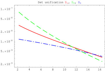
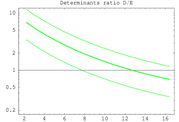
Figure 2: Renormalization of Yukawa determinants, from $M_{Z}$ to $M_{GUT}$ in the MSSM, assuming $\mathop{\rm tan}\beta\simeq 8$. The left plot shows the three Yukawa determinants for U (red, continuous), D (green, dashed), E (blue, dot-dashed). The right plot is more quantitative and shows the D/E ratio, with the one-sigma uncertainty. It becomes compatible with 1 beyond $10^{8}\,\mbox{GeV}$.

3 Model realization: Rank-1 combinations in flavour space

In this section we describe a model that realizes the above ideas in the framework of SO(10) SUSY GUT with SU(3) flavour symmetry. The question to be answered is “what in this framework generates fermion mass hierarchies and flavour mixing?”. Indeed one can use the fact that some hierarchic parameters are generated by the SO(10) breaking: they distinguish between the U, D, E sectors, but independently of the flavour. Then one can imagine that when flavour is broken these hierarchic parameters will be assigned to the correct direction, i.e. large ones in the third family direction in all fermion sectors. Since the unification of determinants observed in the previous section seems to suggest that some relations among eigenvalues may not depend on the fermion sector, and also do not depend on the flavour mixing, we can then try to think that in first approximation it is possible to disentangle the hierarchy of eigenvalues from the mixing structure, that in turn can be common to the U, D, E sectors. Once a flavour breaking is introduced it will not only generate mixings, but, if it is not just unitary matrices, it will also modify slightly the eigenvalues, and thus will generate the deviations $A_{e,d}$.

Following [8] we review here how these ideas can be implemented, writing the Yukawa matrices at GUT scale as a hierarchic combination of three fixed rank-one projectors in flavour space. This approach was devised in [4, 5] as a description of an inverse hierarchy unification at very low $\mathop{\rm tan}\beta$, as in the first case of figure 1. It turns out however that it is quite successful in accounting for fermion masses and mixings even at moderate $\mathop{\rm tan}\beta$, in fact it is even more successful.

Let us start with the case of no mixings and ignoring the deviations from strict hierarchy. As mentioned in the beginning, it is clear that this case is quite simple, and one would build a model that produces the following Yukawa matrices:

$$\hat{\lambda}_{f}^{\rm{no\ mix}}\!\!\! = {}\lambda\,\left[\epsilon_{f}\left(\begin{array}[]{ccc}1&0&0\\ 0&0&0\\ 0&0&0\end{array}\right)\,+\left(\begin{array}[]{ccc}0&0&0\\ 0&1&0\\ 0&0&0\end{array}\right)\,+\epsilon_{f}^{-1}\left(\begin{array}[]{ccc}0&0&0\\ 0&0&0\\ 0&0&1\end{array}\right)\right],\quad f=u,d,e$$ (24)

with $\epsilon_{e,d}\simeq 1/50$ and $\epsilon_{u}\simeq 1/500$. Notice that the determinant here is independent of the fermion sector $f$, i.e. $\det\lambda_{f}=\lambda^{3}$, while the eigenvalues follow different hierarchies in different sectors. Unification of determinants follows from choosing {$\epsilon_{f}$, 1, $\epsilon_{f}^{-1}$} coefficients. This form ignores the deviations as well as the mixings, but the reason of this is evident: three chosen matrices are mutually orthogonal projectors.

One is therefore led to consider a modification of the above, using the most general rank-one projectors, in place of orthogonal ones. It is necessary that they are rank-one, because the eigenvalues should reflect the hierarchy of the $\epsilon_{f}$.

The Yukawa matrices are thus taken as a hierarchic combination of three generic rank-one projectors in flavour space $\hat{P}_{1,2,3}$:

$$\hat{\lambda}_{f} = {}\lambda\,\Big{[}\epsilon_{f}\,\hat{P}_{1}\,+\hat{P}_{2}\,+\epsilon_{f}^{-1}\,\hat{P}_{3}\Big{]}\,,\qquad f=u,d,e,\nu_{D}$$ (25)

where we have included also the Yukawa matrix for neutrinos, that will anyway be present in SO(10) unification, and we will consider it later. The $\hat{P}_{n=1,2,3}$ are three generic rank-one complex matrices and may be parametrized as $\hat{P}_{n}=p_{n}\otimes p^{\prime}_{n}=p_{n}{p^{\prime}}_{n}^{t}$, with $p_{n}$, $p^{\prime}_{n}$ three couples of vectors in flavour space (flavour triplets). The $p_{n}$ and $p^{\prime}_{n}$ may be realized as the VEV of flavour triplets, and may be thought as providing the ’left’ and ’right’ flavour structures. They are thus responsible for the breaking of the SU(3) flavour symmetry, and this breaking does not depend on the fermion sector. Once both SO(10) and SU(3) are broken, the $\epsilon_{f}$ hierarchies are mixed via the $\hat{P}_{n}$’s to generate both almost hierarchic eigenvalues as well as mixing angles.

In this way one has a cooperation of the gauge (vertical) and flavour (horizontal) sectors, of the theory, while allowing quite general mass matrices.

Looking at the determinant of these $\hat{\lambda}_{f}$ matrices, it turns out to factorize as:

$$\det\hat{\lambda}_{f}\;=\;\lambda^{3}\,D_{p}\,D_{p^{\prime}}\,,$$ (26)

with $D_{p}=p_{1}\cdot(p_{2}\wedge p_{3})$ and similarly for $D_{p^{\prime}}$. This is again independent of $\epsilon_{f}$, i.e. the determinants are unified in the U, D, E, $\nu$ sectors and the eigenvalues follow the predictions of the previous sections, independently of the parameters entering in $p_{n}$ and $p^{\prime}_{n}$.

To see in detail how this ansatz works, we choose a flavour basis and we restrict for simplicity to the case of symmetric projectors for example assuming that $p^{\prime}_{n}=p_{n}$ are the VEV of the same triplet:

$$\lambda_{f}=\lambda\Big{[}\epsilon_{f}\hat{P}_{1}\,+\hat{P}_{2}\,+\epsilon_{f}^{-1}\hat{P}_{3}\Big{]} \!\!=\!\! \lambda\left[\epsilon_{f}\left(\begin{array}[]{ccc}1&a&b\\ a&a^{2}&ab\\ b&ab&b^{2}\end{array}\right)+\!\left(\begin{array}[]{ccc}0&0&0\\ 0&1&c\\ 0&c&c^{2}\end{array}\right)+\epsilon_{f}^{-1}\left(\begin{array}[]{ccc}0&0&0\\ 0&0&0\\ 0&0&d^{2}\end{array}\right)\right]$$ (36)

$$\!\!=\!\! \lambda\left(\begin{array}[]{ccc}\epsilon_{f}&a\,\epsilon_{f}&b\,\epsilon_{f}\\[4.30554pt] a\,\epsilon_{f}&1+a^{2}\epsilon_{f}&c+ab\,\epsilon_{f}\\[4.30554pt] b\,\epsilon_{f}&c+ab\,\epsilon_{f}&d^{2}/\epsilon_{f}+c^{2}+b^{2}\epsilon_{f}\end{array}\right)\,,$$ (40)

where we have rotated globally all the $p_{n}$ vectors in flavour space and rescaled $\epsilon_{f}$, $\lambda$ to set $p_{1}=(1,a,b)$, $p_{2}=(0,1,c)$, $p_{3}=(0,0,d)$. Eliminating also the irrelevant phases, we end up with the following generic 13 parameters domain: $\lambda,a,d\in{\mathbb{R}}^{+}$, $b,c,\epsilon_{u},\epsilon_{d},\epsilon_{e}\in{\mathbb{C}}$. These parameters should account for all Dirac couplings of charged fermions.

It is also worth displaying an other form of this matrix

$$\hat{\lambda}_{f} = {}\lambda\,\hat{T}\left(\begin{array}[]{ccc}\epsilon_{f}&0&0\\ 0&1&0\\ 0&0&\epsilon_{f}^{-1}\end{array}\right)\hat{T}^{\,t}\,,\qquad\hat{T}=\left(\begin{array}[]{c|c|c}&&\\ p_{1}&p_{2}&p_{3}\\ &&\end{array}\right)=\left(\begin{array}[]{ccc}1&0&0\\ a&1&0\\ b&c&d\end{array}\right),$$ (50)

where we can see that the flavour breaking triplets $p_{n}$ induce a flavour mixing through $\hat{T}$ that is not unitary, and therefore will induce not only mixing angles, but also deviations in the eigenvalues. The deviations will therefore be linked to the flavour mixing. This form is also useful to easily prove (26).

3.1 Leading order analysis

The form (36) can be taken as an ansatz and can be solved quite completely by computing the leading order expressions of eigenvalues and mixing angles:

$$\lambda_{u}\simeq\lambda\,|\epsilon_{u}|\,,\ \ \qquad\quad \lambda_{c}\simeq\lambda\,,\quad\ \ \ \ \ \ \qquad\qquad\lambda_{t}\simeq\lambda\left|\frac{d^{2}}{\epsilon_{u}}\right|$$ (51)

$$\lambda_{d}\simeq\lambda\frac{|\epsilon_{d}|}{|1+{a^{2}\epsilon_{d}}|}\,,\quad \lambda_{s}\simeq\lambda|1+{a^{2}\epsilon_{d}}|\,,\quad\qquad\lambda_{b}\simeq\lambda\left|\frac{d^{2}}{\epsilon_{d}}\right|$$ (52)

$$\lambda_{e}\simeq\lambda\frac{|\epsilon_{e}|}{|1+{a^{2}\epsilon_{e}}|}\,,\quad \lambda_{\mu}\simeq\lambda|1+{a^{2}\epsilon_{e}}|\,,\quad\qquad\lambda_{\tau}\simeq\lambda\left|\frac{d^{2}}{\epsilon_{e}}\right|$$ (53)

$$\theta_{12}\simeq-\frac{a\epsilon_{d}}{1+a^{2}\epsilon_{d}}\,,\qquad\theta_{23}\simeq\frac{\eta_{d}}{d^{2}}\epsilon_{d}\,,\qquad\theta_{13}\simeq\frac{b}{d^{2}}\epsilon_{d}^{2}\,,\qquad\gamma_{CP}\simeq\arg\left(\frac{b(1+a^{2}\epsilon_{d})}{\eta_{d}}\right).$$ (54)

where $\eta_{d}=(c+ab\,\epsilon_{d})$, and since $\epsilon_{u}\ll\epsilon_{d,e}$, the quark mixing angles are well approximated by the “down” sector. We will not repeat the whole analysis that can be found in [8] but just quote the main steps that demonstrate how the horizontal and vertical hierarchy cooperate.

• First from $\lambda_{b}\simeq\lambda_{\tau}$, one should have $|\epsilon_{e}|\simeq|\epsilon_{d}|$ as already discussed.

• Second, one notes that, ignoring the corrections, the second generation Yukawa are unified $\lambda_{c,s,\mu}\simeq\lambda$.

• However, the RG invariant relation $s_{12}\simeq\sqrt{m_{d}/m_{s}}$ tells us that $|a^{2}\epsilon_{d}|\simeq 1$, so that $a$ should actually be quite large, $|a|\sim|\epsilon_{d}|^{-1/2}$ ($\simeq 7$, see later).

  This large value of $a$ generates the right Cabibbo angle, but also enters the correction of the eigenvalues in the first two generations of D, E sectors.

• Indeed right splitting of s,$\mu$ Yukawa is produced by the factors $A_{d,e}=|1+a^{2}\epsilon_{d,e}|$ once the sign (the phases) of $a^{2}\epsilon_{e}$ and $a^{2}\epsilon_{d}$ are nearly opposite, $a^{2}\epsilon_{e}\simeq-a^{2}\epsilon_{d}\simeq\mbox{e}^{0.5i}$, so that $|A_{e}|\simeq 2$, $|A_{d}|\simeq 0.5$. As discussed above, for the first generation the split goes (correctly) in the opposite direction, realizing the small flavour seesaw.

  So, in this ansatz, the largeness of $a$, following from the Cabibbo angle, explains also the deviation from exactly hierarchical family masses of $e$, $d$, $\mu$, $s$. This was already observed in [4].

• From other known mass ratios one can then determine $|\epsilon_{e,d}|\simeq 1/55$, $a\simeq 7.5$, $|\epsilon_{u}|\simeq 1/600$, $d^{2}\simeq 0.5$, $\mathop{\rm tan}\beta\simeq 7.3$. Then further insight can be gained by checking the CP phase and the other mixing angles: from these it turns out that also $b$ is quite large, like $a$, i.e. $|b|\simeq 5$. Also, one finds two branches: in one the complex $b$ and $c$ are almost orthogonal, in the other they are opposite. Finally, there is a flat direction, a combination of $|\epsilon_{e}/\epsilon_{d}|$ with the common phase of $b$, $c$.

Summing up, the ansatz is solved successfully and shows a one parameter family of solutions, with two branches. The precise leading-order solution for all parameters is not conclusive since next-to-leading corrections and contributions to CKM from the “up” sector are 10% in magnitude, larger than experimental errors; hence a numeric fit is necessary and will be described below. Nevertheless the ansatz is capable of accounting for all the charged fermion masses and mixings, unifying the determinants and giving an additional mechanism that links the deviations $A_{e,d}$ with the Cabibbo angle $\theta_{12}$.

Before describing a model that realizes this ansatz, we would like to comment on the solution found from the charged fermions so far. Collecting the three $p_{n}$ vectors:

$$p_{1}=(1,\,7,\,5)\,,\qquad p_{2}\simeq(0,\,1,\,0.2\mbox{--}1.5)\,, \qquad p_{3}\simeq(0,\,0,\,0.7)\,,$$ (55)

we observe that they tend to lie in the 2-3 plane. Exact planarity is broken to order $1/8\simeq\sqrt{\epsilon_{d}}$, as can be seen from the first 1 with respect to the modulus of its vector $|p_{1}|\simeq 8.5$. The reason for this is to be tracked in the magnitude of the quark mixing angles that require $a$ and $b$ to be large while $c$ and $d$ are of order one.

We find this pattern of quasi-planar triplets a nice hint for the realization of a flavour sector of the theory, where the $p_{n}$ vectors are generated by the VEV of three scalar fields that are triplets of the flavour SU(3). The potential and the radiative corrections to it lead to their mutual disorientation, along the liens of [12, 13]. Incidentally, we also note that while we started from complex triplets, fitting fermion masses and mixings indicates that the only two complex parameters $b$, $c$ have a common phase. This means that the three triplets VEV can be taken completely real. The CP violation is then produced just by the complex $\epsilon_{f}$ and the coupling constants. This is most welcome, since in usual VEV configurations, the triplets tend to repel or attract each other and it is hard to obtain complex relative angles. We leave this analysis and the realization of the flavour sector for future work.

In the next section we complete the description of the model in the SO(10) side, where the rank-one projectors are mixed with the SO(10) breaking VEVs that generate the hierarchy parameters.

4 SO(10) universal seesaw and flavour

Since the different $\epsilon_{u,d,e}$ hierarchies correspond to a broken SO(10), it is natural to generate them at SO(10) breaking, i.e. at the GUT scale, and then transfer them in some way to the light fermions-higgs Yukawa couplings. At the GUT scale we should also mix them with the flavour triplets VEVs $p_{n}$ mentioned above. We describe here a way to implement this program, along the lines of [5, 8].

4.1 Small parameters from SO(10) breaking

First we recall that among the different schemes of SO(10) breaking, a very successful and economical one is that implementing the so called missing-VEV mechanism [14], that while breaking to the SM gauge group, automatically stabilizes the hierarchy of the light doublets with respect to the GUT scale. Among other fields, in this mechanism there are three multiplets in the $\mathbf{45}$ representation: $\mathbf{45}_{X}$, $\mathbf{45}_{R}$, $\mathbf{45}_{BL}$. Altogether they break SO(10) to the SM group, therefore their VEVs are, in Pati-Salam notation, only allowed along the two directions $(\mathbf{15},\mathbf{1},\mathbf{1})$ and $(\mathbf{1},\mathbf{1},\mathbf{3})$. It turns out that $\langle\mathbf{45}_{R}\rangle\in(\mathbf{1},\mathbf{1},\mathbf{3})$, $\langle\mathbf{45}_{BL}\rangle\in(\mathbf{15},\mathbf{1},\mathbf{1})$ and $\langle\mathbf{45}_{X}\rangle\in(\mathbf{15},\mathbf{1},\mathbf{1})+(\mathbf{1},\mathbf{1},\mathbf{3})$.

All these VEVs can be used in a ratio to some higher scale (e.g. $M\sim 10^{17}\mbox{GeV}$) to introduce small parameters into the game. However the last one, the VEV of $\mathbf{45}_{X}$, is of particular interest since it depends generically on two coefficients, that define its mixture of $(\mathbf{15},\mathbf{1},\mathbf{1})$ and $(\mathbf{1},\mathbf{1},\mathbf{3})$. When the small ratio $\langle\mathbf{45}_{X}\rangle/M$ is projected onto the fermion multiplets and it decomposes in four small parameters $\epsilon_{u}$ $\epsilon_{d}$ $\epsilon_{e}$ $\epsilon_{\nu_{D}}$, we have that only two of these are independent, and they turn out [5] to be constrained by the following relations:

$$\epsilon_{e}=-\epsilon_{d}-2\epsilon_{u}\,,\qquad\epsilon_{\nu_{D}}=-2\epsilon_{d}-\epsilon_{u}\,.$$ (56)

The first equation tells us that once $|\epsilon_{u}|\ll|\epsilon_{d}|$, the equality in the D,E sectors $|\epsilon_{e}|\simeq|\epsilon_{d}|$ is predicted, nicely reproducing the pattern observed in nature. Moreover, the same relation implies also bottom-tau unification, with a deviation of $\epsilon_{u}/\epsilon_{e}\simeq 10\%$, that is indeed observed.

The second equation gives a prediction on the Yukawa hierarchy in the neutrino sector, and implies that it is milder than that of the leptons, $\epsilon_{\nu_{D}}\simeq 1/25$.

Therefore without introducing new fields in the theory, we found that the $\mathbf{45}_{X}$ generates the right pattern of small hierarchy parameters $\epsilon_{u}$, $\epsilon_{d}$, $\epsilon_{e}$, $\epsilon_{\nu_{D}}$. For this reason we will assume below that the flavour hierarchies are generated as effective operators by powers of $\langle\mathbf{45}_{X}\rangle/M$.

4.2 SO(10) universal seesaw

To generate the Yukawa couplings as the correct effective operators, it is necessary to introduce new (super)heavy fermion multiplets, that act as messengers. Let us start with three families of heavy vectorlike fermions $\mathbf{16}^{\prime}_{i}$, $\overline{\mathbf{16}}^{\prime}_{i}$. To generate the light Yukawa couplings they should couple both to the light fermions and to the Higgs field, that we take to be the usual $\mathbf{10}=T(\mathbf{6},\mathbf{1},\mathbf{1})+\phi(\mathbf{1},\mathbf{2},\mathbf{2})$. This contains the MSSM higgses in $\phi$. The three families of light fermions then receive an effective Yukawa coupling matrix from the mass matrix of heavy vectorlike fermions $\mathbf{16}^{\prime}_{i}$, $\overline{\mathbf{16}}^{\prime}_{i}$, via a “universal” seesaw mechanism [9]. In detail, the superpotential contains

$$W=\gamma\,\mathbf{10}\,\mathbf{16}^{i}\mathbf{16}^{\prime}_{i}\,+\gamma^{\prime}\,\mathbf{45}_{R}\,\mathbf{16}^{i}\,\overline{\mathbf{16}}^{\prime}_{i}\,+\overline{\mathbf{16}}^{\prime}_{i}\,M_{heavy}^{ij}\mathbf{16}^{\prime}_{j}$$ (57)

where $\mathbf{10}$ is the fundamental Higgs and $\mathbf{45}_{R}$ is an adjoint one whose role will be clear in a moment. Notice that by SU(3) flavour symmetry a direct Yukawa coupling $\mathbf{16}\mathbf{16}\mathbf{10}$ is forbidden. The flavour structure is encoded in $\hat{M}_{heavy}$, while the first two terms are flavour universal. Near at the GUT scale, the higgses develop a VEV, so that the heavy fermions $\mathbf{16}^{\prime}$ decouple and the light fermions $\mathbf{16}$ acquire an effective Yukawa coupling with $\mathbf{10}$ that is approximately given by the “seesaw” formula:

$$\hat{\lambda}=\gamma\,\gamma^{\prime}\,\langle\mathbf{45}_{R}\rangle\,\hat{M}_{heavy}^{-1}\,,$$ (58)

Therefore the Yukawa couplings of the light fermions $\lambda$ are proportional to the inverse of the heavy fermion masses, that in turn should exhibit an inverted hierarchy pattern, with the lightest particle being the heavy correspondent of the “top”.

To make explicit the universal seesaw following from (57), we decompose in Pati-Salam notation the fermion fields as: $\mathbf{16}^{i}=f^{i}(\mathbf{4},\mathbf{2},\mathbf{1})+f^{ic}(\overline{\mathbf{4}},\mathbf{1},\mathbf{2})$ and $\mathbf{16}^{\prime}_{i}={\cal F}_{i}(\mathbf{4},\mathbf{2},\mathbf{1})+F^{c}_{i}(\overline{\mathbf{4}},\mathbf{1},\mathbf{2})$, $\overline{\mathbf{16}}^{\prime}_{i}={\cal F}^{c}_{i}(\overline{\mathbf{4}},\mathbf{2},\mathbf{1})+F_{i}(\mathbf{4},\mathbf{1},\mathbf{2})$. Note that $f=q,l$ and ${\cal F}=q^{\prime},l^{\prime}$ are isospin doublets and $f^{c}=u^{c},d^{c},e^{c},\nu^{c}$, $F=u^{\prime},d^{\prime},e^{\prime},\nu^{\prime}$, are isospin singlets. With this decomposition the couplings can be illustrated as follows:

$$\begin{array}[]{ccc}&{\begin{array}[]{ccc}\,f^{c}&\,\,\,\;F^{c}&\,\,\;{\cal F}^{c}\end{array}}\\ \vspace{2mm}\begin{array}[]{c}f\\ F\\ {\cal F}\end{array}\!\!\!\!\!&{\left(\begin{array}[]{ccc}0&{\gamma}\phi&0\\ {M}_{R}&\hat{M}_{F}&0\\ {\gamma}\phi&0&\hat{M}_{\cal F}\end{array}\right)}\end{array}\vspace*{-1ex}$$

where $M_{R}$ is the scale of $\langle\mathbf{45}_{R}\rangle$ and $\hat{M}_{heavy}$ is decomposed in $\hat{M}_{F}$ and $\hat{M}_{\cal F}$ , respectively the mass matrices of heavy isosinglets and isodoublets (unmixed).

Only the $F$, $F^{c}$ participate in the decoupling process and in each sector the Yukawa matrix is proportional to the inverse of $\hat{M}_{F}$ alone:

$$\hat{\lambda}_{f}=\gamma\,M_{R}\,\hat{M}_{F}^{-1}\,,\hbox to0.0pt{$\qquad\qquad f=u,d,e,\nu_{D}\,.$\hss}$$ (59)

Figure 3: Universal seesaw mechanism using $\mathbf{45}_{R}$.

It is important to note that the $f$-${\cal F}^{c}$ entry is zero because $\langle\mathbf{45}_{R}\rangle$ is in the “right” direction. This shows three remarkable features of this universal seesaw using $\mathbf{45}_{R}\in(\mathbf{1},\mathbf{1},\mathbf{3})$: 1) only the isosinglets $F^{c}$ participate in the seesaw mixing with $f^{c}$, so that their mass matrix is directly reproduced in the light Yukawa; this avoids a mixing with $M_{\cal F}$ that could spoil the exact hierarchies; 2) the LLLL (dominant) part of the D=5 proton decay is automatically eliminated, because ($\mathbf{1}$,$\mathbf{1}$,$\mathbf{3}$) does not couple the light and heavy isodoublets [5, 10]; 3) finally, again because the heavy isodoublets do not enter the seesaw, the squark and sleptons mass matrices are automatically aligned with the (square of the) Yukawa matrices, and this eliminates problems of flavour changing neutral currents. We conclude that here the universal seesaw via the SU(2)_R breaking automatically allows the correct mass generation, suppresses proton decay and SUSY flavour problems.

4.3 Entangling flavour and SO(10) higgses

We now come to the generation of the flavour structure in $\hat{M}_{heavy}$. We have already introduced the three flavour projectors $P_{n}$ that should be coupled to different powers of the $\mathbf{45}_{X}$ field. Since however from (58), (59) the heavy mass matrix is the inverse of the Yukawa couplings, we must take advantage of a property of combinations of rank-one projectors: the inverse of such a combination is a combination of new projectors, with inverse coefficients:

$$\big{(}\alpha_{1}\hat{P}_{1}+\alpha_{2}\hat{P}_{2}+\alpha_{3}\hat{P}_{3}\big{)}^{-1}=\left(\frac{1}{\alpha_{1}}\hat{Q}_{1}+\frac{1}{\alpha_{2}}\hat{Q}_{2}+\frac{1}{\alpha_{3}}\hat{Q}_{3}\right),$$ (60)

where the $\hat{Q}_{n}$ are the “reciprocal” of the $\hat{P}_{n}$ projectors: if $\hat{P}_{n}$ are parametrized with flavour triplets as $\hat{P}_{n}=p_{n}p_{n}^{t}$, then $\hat{Q}_{n}=q_{n}q_{n}^{t}$ are given by three new triplets $q_{n}$ that are in fact the reciprocal of the $p_{n}$ ones: $q_{n}=\frac{1}{2}\epsilon_{nmr}p_{m}\wedge p_{r}/D_{p}$, with $D_{p}=p_{1}\cdot(p_{2}\wedge p_{3})$.

Therefore one should generate a $\hat{M}_{heavy}$ as a combination of three rank-one projectors $Q_{n}$ multiplied by powers of $\mathbf{45}_{X}/M$. To have hierarchic eigenvalues these should be successive powers, i.e.:

$$\hat{M}_{heavy}\propto\Big{[}\hat{Q}_{1}+\frac{\mathbf{45}_{X}}{M}\hat{Q}_{2}+\frac{\mathbf{45}_{X}^{\!2}}{M^{2}}\hat{Q}_{3}\Big{]}\,,$$

We do not specify at this point the effective realization of this operator, that will be addressed later on. We only observe that such effective operators may involve integer powers (positive or negative) of fields, and therefore one may have in front a generic power of it:

$$\hat{M}_{heavy}\propto\Big{(}\frac{\mathbf{45}_{X}}{M}\Big{)}^{\!-n}\Big{[}\hat{Q}_{1}+\frac{\mathbf{45}_{X}}{M}\hat{Q}_{2}+\frac{\mathbf{45}_{X}^{\!2}}{M^{2}}\hat{Q}_{3}\Big{]}\,,$$ (61)

It is clear that when at SO(10) breaking $\langle\mathbf{45}_{X}\rangle/M$ generates the small parameters $\epsilon_{u}$, $\epsilon_{d}$, $\epsilon_{e}$, $\epsilon_{\nu_{D}}$, one will receive effective Yukawa couplings in the form:

$$\hat{\lambda}_{f}=\frac{\epsilon_{f}^{n-2}}{\lambda}\big{[}\epsilon_{f}^{2}P_{1}+\epsilon_{f}P_{2}+P_{3}\big{]}\qquad\qquad f=u,d,e,\nu_{D}$$ (62)

The interesting cases are $n=0$,$1$,$2$, that correspond to the three cases of figure 1:

• with $n=0$, the coefficients are $1,\epsilon_{f}^{-1},\epsilon_{f}^{-2}$, and the GUT Yukawa couplings of the first generation are approximately unified. This requires very low $\mathop{\rm tan}\beta$ ($<2$);

• with $n=1$, the coefficients are $\epsilon_{f},1,\epsilon_{f}^{-1}$, we have an approximate unification of the second generation, at intermediate $\mathop{\rm tan}\beta$ ($\simeq 10$);

• with $n=2$, the coefficients are $\epsilon_{f}^{2},\epsilon_{f}^{,}1$, and large $\mathop{\rm tan}\beta$ ($>50$), one reaches unification of the third generation, as in the known case of t-b-$\tau$ unification.

The second case is the most interesting since there is optimal agreement with the data, and as discussed in the present work, the determinants are unified. For the first case see [5], for a unified treatment see [8].

Sticking to the interesting case of n=1 (b), we end this section by providing the complete realization with renormalizable operators. Such a realization is not unique, so we display two different ways to achieve the same result.

Every realization of nonrenormalizable operators like (61) requires one to introduce additional fields. For example one can introduce four more vector-like fermion multiplets that are flavour singlets: $\mathbf{16}^{\prime\prime}_{1}$, $\mathbf{16}^{\prime\prime}_{2}$, $\mathbf{16}^{\prime\prime}_{3}$ and $\mathbf{16}^{\prime\prime\prime}$ (and their conjugates); as an other example one can use in place of three triplets $q_{n}$, two triplets $q_{1,2}$ plus one sextet $\chi_{3}$, and then introduce three vector-like fermion fields: two flavour singlets $\mathbf{16}^{\prime\prime}_{1,2}$ and one triplet $\mathbf{16}^{\prime\prime\prime i}$ (and their SO(10)$\times$SU(3) conjugates). The coupling are arranged as follows in these two cases:

$$\begin{array}[t]{l|cccccc|}&\mathbf{16}^{i}&\mathbf{16}^{\prime}_{i}&\mathbf{16}^{\prime\prime}_{1}&\mathbf{16}^{\prime\prime}_{2}&\mathbf{16}^{\prime\prime}_{3}&\mathbf{16}^{\prime\prime\prime}\\ \hline\cr\mathbf{16}^{i}&&\mathbf{10}&&&&\\ \overline{\mathbf{16}}^{\prime}_{j}&\mathbf{45}_{R}&&q_{1}^{j}&q_{2}^{j}&q_{3}^{j}&0\\ \overline{\mathbf{16}}^{\prime\prime}_{1}&&q_{1}^{i}&\mathbf{45}_{X}&&&\\ \overline{\mathbf{16}}^{\prime\prime}_{2}&&q_{2}^{i}&&{M}&&\\ \overline{\mathbf{16}}^{\prime\prime}_{3}&&q_{3}^{i}&&&&{M}\\ \overline{\mathbf{16}}^{\prime\prime\prime}&&0&&&{M}&\mathbf{45}_{X}\\ \hline\cr\end{array}\qquad\begin{array}[t]{l|ccccc|}&\mathbf{16}^{i}&\mathbf{16}^{\prime}_{i}&\mathbf{16}^{\prime\prime}_{1}&\mathbf{16}^{\prime\prime}_{2}&\mathbf{16}^{\prime\prime\prime\,i}\\ \hline\cr\mathbf{16}^{j}&&\mathbf{10}&&&\\ \overline{\mathbf{16}}^{\prime}_{j}&\mathbf{45}_{R}&&q_{1}^{j}&q_{2}^{j}&\mathbf{45}_{X}\\ \overline{\mathbf{16}}^{\prime\prime}_{1}&&q_{1}^{i}&\mathbf{45}_{X}&&\\ \overline{\mathbf{16}}^{\prime\prime}_{2}&&q_{2}^{i}&&{M}&\\ \overline{\mathbf{16}}^{\prime\prime\prime}_{j}&&\chi_{3}^{ij}&&&{M}\\ \hline\cr\end{array}$$

In the first example $q_{n}$ define exactly the three reciprocal triplets mentioned above, while in the second the $\hat{Q}_{1,2,3}$ projectors will be given by $\hat{Q}_{1}\propto q_{1}q_{1}^{t}$, $\hat{Q}_{2}\propto q_{2}q_{2}^{t}$ and $\hat{Q}_{3}\propto\chi_{3}$.

One final remark is in order: in these examples some of the couplings are forbidden. We do not address here the way to motivate this, that can be done by means of additional symmetries, discrete or continuous. Indeed the way that heavy higgses and flavour triplets/sextets are coupled in these examples (and e.g. in (61)) points towards a further symmetry that explains the charges or couplings much in the Froggatt-Nielsen spirit.

5 Neutrinos

In this section we analyze how the neutrino sector can be accommodated in the present framework of flavour triplets coupled with SO(10) heavy Higgs fields. From the mechanism described above, the Dirac neutrino masses are unified together with the other fermions and thus result in the range 10–1000MeV. Therefore we need to introduce also a Majorana mass for right-handed neutrinos, and generate the light neutrino mass by canonical seesaw [11]. Then given that in the model the flavour structure is encoded in the three ${P}_{n}$ projectors, we assume that also the Majorana masses are built with the same projectors.

The Majorana mass for the RH neutrinos that belong to the light $\mathbf{16}$ multiplet is generated via an universal seesaw similar to that of Yukawa couplings, this time via a singlet messenger. We do not dwell in the details that may be found in [8], and we quote the result, that also the RH neutrino mass $\hat{M}_{\nu_{R}}$ will be built with the same flavour projectors $P_{n}$ and with a new hierarchic parameter $\epsilon_{\nu_{R}}$. The coefficients however are generic, since the three new coupling constants can no more be absorbed in the $P_{n}$. We choose to make explicit the $\epsilon_{\nu_{R}}$ and add a further complex parameter $\alpha$.

$$\hat{\lambda}_{\nu_{R}}\propto\Big{[}{\hat{P}}_{1}+\epsilon_{\nu_{R}}{\hat{P}}_{2}+\frac{\epsilon_{\nu_{R}}^{2}}{\alpha}{\hat{P}}_{3}\Big{]}\,,$$ (63)

where for simplicity here and in the following we prefer to use the dimensionless matrices $\hat{\lambda}_{\nu_{R},\nu_{L}}=\hat{M}_{\nu_{R},\nu_{L}}/v\sin\beta$, with the electroweak $v=174\,\mbox{GeV}$.

A mass matrix for the left-handed neutrinos is then generated by canonical seesaw as $\hat{\lambda}_{\nu}=\hat{\lambda}_{\nu_{D}}\hat{\lambda}_{\nu_{R}}^{-1}\hat{\lambda}_{\nu_{D}}$, between the neutrino yukawa (36) and the RH mass matrix (63). The result can be found by exploiting an other interesting property of rank-one combinations: indeed, the following “seesaw” relation holds:

$$\big{(}\alpha_{1}\,\hat{P}_{1}+\alpha_{2}\,\hat{P}_{2}+\alpha_{3}\,\hat{P}_{3}\big{)}\big{(}\beta_{1}\,\hat{P}_{1}+\beta_{2}\,\hat{P}_{2}+\beta_{3}\,\hat{P}_{3}\big{)}^{-1}\big{(}\alpha_{1}\,\hat{P}_{1}+\alpha_{2}\,\hat{P}_{2}+\alpha_{3}\,\hat{P}_{3}\big{)}=$$

$$=\left(\frac{\alpha_{1}^{2}}{\beta_{1}}\,\hat{P}_{1}+\frac{\alpha_{2}^{2}}{\beta_{2}}\,\hat{P}_{2}+\frac{\alpha_{3}^{2}}{\beta_{3}}\,\hat{P}_{3}\right),$$ (64)

i.e. the seesaw acts on the coefficients only, but does not change the flavour projectors $\hat{P}_{n}$. Hence, we get that $\hat{\lambda}_{\nu_{L}}$ is built again as a combination of the same flavour projectors:

$$\hat{\lambda}_{\nu_{L}}=\hat{\lambda}_{\nu_{D}}\hat{\lambda}_{\nu_{R}}^{-1}\hat{\lambda}_{\nu_{D}}\propto\Big{[}\epsilon_{\nu}^{2}\hat{P}_{1}+\epsilon_{\nu}\hat{P}_{2}+\alpha\hat{P}_{3}\Big{]}\,,\qquad\epsilon_{\nu}=\frac{\epsilon_{\nu_{D}}^{2}}{\epsilon_{\nu_{R}}}\,.$$ (65)

Using the explicit form (36), we can rewrite:

$$\lambda_{\nu}\propto\left(\begin{array}[]{ccc}|\epsilon_{\nu}/\bar{A}_{\nu}|&|a\epsilon_{\nu}/A_{\nu}|&|b\epsilon_{\nu}/A_{\nu}|\\ |a\epsilon_{\nu}/A_{\nu}|&1&\hbox to0.0pt{$\rho$\hss}\mbox{\phantom{$\rho^{2}+\sigma$}}\\ |b\epsilon_{\nu}/A_{\nu}|&\rho&\rho^{2}+\sigma\end{array}\right).$$

with $A_{\nu}=(1+a^{2}\epsilon_{\nu})$,  $\rho=(c+ab\epsilon_{\nu})/A_{\nu}$,  $\sigma=(d^{2}\alpha+(b-ac)^{2}\epsilon_{\nu}^{2})/A_{\nu}$.

In this matrix, we only have two free complex parameters $\epsilon_{\nu}$ and $\alpha$, therefore the model is quite constrained since it must explain the neutrino mass hierarchy and the three mixing angles.

Unlike the case of charged fermions, an exact analytical solution of this matrix is not possible, due to the large neutrino mixings and to the small but important uncertainties in the parameters determined from the charged fermions. Nevertheless it is possible to see that neutrinos are predicted to be hierarchic, non degenerate, and to derive a prediction for the $\theta_{13}$ mixing angle. The analysis goes as follows:

• Non-degenerate neutrinos with $m_{\nu 2}/m_{\nu 3}\simeq 1/5$ follow from the fact that $a$ is large, so the ratio of the 1-1 with the 1-2, 1-3 entries is small $\simeq 1/7$.

• Non-zero $\theta_{e3}$ follows from $a>b$, so that the 1-2 entry is larger than the 1-3 one. An analytical estimate of the angles from the 2,3 sector can be given first in the form of a relation between them, using the parameters found from the charged sector and after imposing maximal $\theta_{atm}$:

  $$\frac{\theta_{e3}}{\theta_{sol}}=\frac{m_{\nu 2}}{m_{\nu 3}}\,\Big{|}\frac{1+R\,{\rm e}^{i\delta}}{1-R\,{\rm e}^{i\delta}}\Big{|}\,,\qquad\mbox{with }\ R=\frac{b}{a}\simeq\frac{\theta_{13}^{quark}\lambda_{b}}{\theta_{12}^{quark}\lambda_{s}}\simeq\frac{1}{1.6\thicksim 2.1}\,,$$ (66)

  where $\delta=\arg\rho=\arg[(c+ab\epsilon_{\nu})/(1+a^{2}\epsilon_{\nu})]$. After imposing the correct neutrino hierarchy and solving the model for $\epsilon_{\nu}$, we can estimate also:

  $$\theta_{12}\simeq 30^{\circ}\Big{|}1-R\,{\rm e}^{i\delta}\Big{|}\,,\qquad\theta_{13}\simeq 6^{\circ}\Big{|}1+R\,{\rm e}^{i\delta}\Big{|}\,.$$ (67)

  Hence, choosing ${\rm e}^{i\delta}$ purely imaginary or just slightly negative, we see that the right $\theta_{sol}\simeq 32^{\circ}$ is accomodated, with a prediction for $\theta_{e3}\simeq 4^{\circ}$.

  The precise numbers are sensible to the quark mixing angles and CP-phase, as well as to the neutrino hierarchy. In practice $\theta_{e3}$ can be lowered to reach also $\theta_{e3}\simeq 0.5^{\circ}$ by stretching within 1$\sigma$ the angles and the neutrino hierarchy.

• Finally, a new flat direction emerges, along which the angles and hierarchy do not vary. It directly corresponds to the leptonic CP violation phase, that may be predicted once angles and hierarchy will be known to better accuracy. Also a majorana phase varies along this flat direction.

Summing up, the framework naturally predicts hierarchic neutrinos with nonzero $\theta_{e3}$ in the 1$\sigma$ range, and there is a useful conspiracy from the charged sector to allow the right neutrino pattern. A new flat direction emerges as a combination of the four real parameters, to be added to the one found in the charged leptons sector. Therefore the model effectively takes advantage of just 13 of the 15 real parameters to reproduce the known data.

5.1 Numeric Fit and Results

As mentioned above, we performed in [8] a numerical analysis, taking into account the exact renormalization factors. We performed a best fit of neutrinos together with charged fermions. The $\theta_{e3}$ neutrino mixing, that we have shown to be predicted inside its allowed $1\sigma$ range, is not used as a fit condition, but rather displayed as a model prediction. The fit was performed using the 15 parameters (11 charged fermions, 4 neutrino) against all known data (20 tests).

$$\begin{array}[t]{|c|c|c|l|}\hline\cr&\mbox{exp}&\mbox{fit}&\vrule\lx@intercol\hfil\mbox{pull}\hfil\lx@intercol\vrule\lx@intercol\\ \hline\cr m_{t}&167\pm 5&169&+0.4\\ m_{b}&4.25\pm 0.15&4.4&+0.9\\ m_{c}&1.25\pm 0.1&1.3&+0.4\\ m_{d}&6\pm 2&6.3&+0.1\\ m_{s}&105\pm 25&{\bf 134}&{\bf+1.1}\\ m_{s}/m_{d}&19.5\pm 2.5&21.4&+0.6\\ \mbox{Ellipse}&23\pm 2&{22.1}&{-0.4}\\ m_{u}/m_{d}&0.5\pm 0.2&{\bf 0.25}&{\bf-1.2}\\ m_{u}\!\!+\!m_{d}&8.5\pm 2.5&8.&-0.2\\ \hline\cr m_{e}&0.511&.510&<0.1\\ m_{\tau}&1777&1779&<0.1\\ \hline\cr\end{array}\qquad\begin{array}[t]{|c|c|c|l|}\hline\cr&\mbox{exp}&\mbox{fit}&\vrule\lx@intercol\hfil\mbox{pull}\hfil\lx@intercol\vrule\lx@intercol\\ \hline\cr\theta_{c}&12.7\pm 0.1&12.75&+0.5\\ V_{cb}10^{2}\!\!&4.13\pm 0.15&4.14&<0.1\\ V_{ub}10^{3}\!\!&3.7\pm 0.47&3.77&+0.2\\ \sin\!2\beta_{CP}&0.736\pm 0.05&0.734&-0.1\\ \gamma_{CP}&1.03\pm 0.22&1.07&+0.2\\ \hline\cr\theta_{sol}&32\pm 3&32.03&<0.1\\ \theta_{atm}&45\pm 7&44.1&<0.1\\ h_{\nu}&0.18\pm 0.07&0.185&<0.1\\ \hline\cr\hline\cr\theta_{e3}&0^{\circ}\mbox{ -- }9.6^{\circ}&0.5\mbox{--}7.0&(br1)\\[-0.68887pt] &&1.7\mbox{--}4.3&(br2)\\ \mathop{\rm tan}\beta&&7.8&\\ \hline\cr\end{array}$$

Table 1: Best fit with $M_{SUSY}=m_{t}$. Total $\chi^{2}=0.35$ per d.o.f.

$$\begin{array}[t]{|c|c|c|l|}\hline\cr&\mbox{exp}&\mbox{fit}&\vrule\lx@intercol\hfil\mbox{pull}\hfil\lx@intercol\vrule\lx@intercol\\ \hline\cr m_{t}&167\pm 5&168&<0.1\\ m_{b}&4.25\pm 0.15&4.4&+0.4\\ m_{c}&1.25\pm 0.1&1.3&+0.4\\ m_{d}&6\pm 2&6.1&+0.4\\ m_{s}&105\pm 25&127&+0.8\\ m_{s}/m_{d}&19.5\pm 2.5&21.0&+0.6\\ \mbox{Ellipse}&23\pm 2&{22.2}&{-0.4}\\ m_{u}/m_{d}&0.5\pm 0.2&{0.32}&{-0.8}\\ m_{u}\!\!+\!m_{d}&8.5\pm 2.5&8.&-0.2\\ \hline\cr m_{e}&0.511&.510&<0.1\\ m_{\tau}&1777&1779&<0.1\\ \hline\cr\end{array}\qquad\begin{array}[t]{|c|c|c|l|}\hline\cr&\mbox{exp}&\mbox{fit}&\vrule\lx@intercol\hfil\mbox{pull}\hfil\lx@intercol\vrule\lx@intercol\\ \hline\cr\theta_{c}&12.7\pm 0.1&12.7&<0.1\\ V_{cb}10^{2}\!\!&4\pm 0.15&4.13&<0.1\\ V_{ub}10^{3}\!\!&3.7\pm 0.47&3.76&+0.2\\ \sin\!2\beta_{CP}&0.736\pm 0.05&0.734&<0.1\\ \gamma_{CP}&1.03\pm 0.22&1.06&+0.1\\ \hline\cr\theta_{sol}&32\pm 3&32.0&<0.1\\ \theta_{atm}&45\pm 7&45.0&<0.1\\ h_{\nu}&0.18\pm 0.07&0.185&<0.1\\ \hline\cr\hline\cr\theta_{e3}&0^{\circ}\mbox{ -- }9.6^{\circ}&0.5\mbox{--}7.0&(br1)\\[-0.68887pt] &&1.6\mbox{--}4.2&(br2)\\ \mathop{\rm tan}\beta&&7.4&\\ \hline\cr\end{array}$$

Table 2: Best fit with $M_{SUSY}=1\,\mbox{TeV}$ total $\chi^{2}=0.14$ per d.o.f.

The best fit results are shown in tables 1 and 2: the overall $\chi^{2}=0.35$ per d.o.f. is quite good, and the model can account for all experimental constraints, albeit having a bit low $m_{u}$ and a bit large $m_{s}$ (1$\sigma$ level) as implied by the predictions described in section 2.

The fit results confirm the analytical study:

• Apart from $m_{u}$, $m_{s}$ that deviate at most 1-$\sigma$, all data are fitted without tension ($<0.3\sigma$).

• The flat direction and the two branches correctly emerge from the fit. In the second branch all complex phases are almost aligned, hinting for a model with complex aligned $\epsilon_{f}$’s and real triplets, with a reduction of the total number of real parameters to 10.

• Neutrinos are predicted as hierarchic and non degenerate, and the mixing from terrestrial neutrinos is nonzero: $\theta_{e3}\simeq 2.5^{\circ},4.9^{\circ}$.

• Neutrino come out hierarchic and non degenerate $m_{\nu}\simeq(0.0045,\,0.01,\,0.048)\,\mbox{eV}$, and right-handed neutrino masses are of the order ($10^{7}$, $10^{9}$, $10^{11}$) GeV.

6 Discussion

In this work we discussed the structure of the Yukawa matrices as renormalized at a common high scale, and in the context of MSSM GUT, noticed the unification of their determinants. This new unification translates in precise predictions in terms of charged fermion masses: in particular it gives a prediction for $m_{d}m_{s}$ in 1$\sigma$ accordance with the experimental ranges, and a prediction of $\mathop{\rm tan}\beta\simeq 7$ that lies in the currently favoured range. In addition this mechanism introduces a constraint that may explain why the first family fermions are light when the third ones are heavy, in a kind of flavour seesaw.

In fact, as opposed to traditional unification schemes, this idea does not unify some combination of yukawa matrices at GUT scale, but unifies approximately the yukawa eigenvalues of the second family.

Examining the mass matrices in more detail we presented an ansatz, similar to the ones put forward in in [4, 5], that realizes the unification of determinants by building the yukawa matrices as hierarchical combinations of three generic rank-one projectors in flavour space. This construction is successful in explaining the deviations from exact mass hierarchy in the D, E sectors, linking them to the Cabibbo mixing.

We reviewed how these ideas can be realized in a predictive model of SU(3) flavour symmetry in the context of SO(10) SUSY GUT, along the lines of [8]. In this model the mass matrices can be analyzed with a leading-order analytical approach and with a complete numerical fit. All fermion masses and mixings are accomodated at 1$\sigma$ level, including neutrinos, for which the analysis and the numerical fit suggest direct and hierarchical neutrinos with non zero $\theta_{e3}=1.7^{\circ}$–$4.3^{\circ}$ or $0.5^{\circ}$–$7^{\circ}$, in two branches.

The model uses the tools that are already available in the context of SO(10) SUSY GUT: a “universal seesaw” mechanism and the higgses present in the missing VEV mechanism. The universal seesaw is used to to transfer the mass matrices from a set of superheavy fermions living near GUT to the ordinary light ones. the higgses in the $\mathbf{45}$ representation that realize the missing VEV mechanism automatically generate the correct horizontal hierarchies $\epsilon_{u}\ll\epsilon_{e,d}$. Then the mass matrices are generated by coupling one of these higgses with three flavour triplets scalar fields, that define three rank-one projectors. This model realization via universal seesaw efficiently suppresses proton decay and SUSY FCNC, and maintains almost pure MSSM content below the GUT scale.

In the flavour sector, the solution emerging from the data-fitting points to quasi-aligned or quasi-planar triplets, that seem to suggest a precise mechanism of SU(3) breaking along VEVs without introducing ad-hoc breakings of flavour, as described for example in [12, 13].

We conclude that the unification of Yukawa determinants at the GUT scale nicely fits into the framework of SO(10) Grand Unification with horizontal symmetries, where it gives a hint for building the flavour sector of the theory, while still giving model independent predictions for the fermion masses and the the $\mathop{\rm tan}\beta$ MSSM parameter.

7 Acknowledgments

This work was partially supported by the MIUR grant under the Projects of National Interest PRIN 2004 ”Astroparticle Physics”.

Appendix A Appendix: MSSM renormalization

In the MSSM, fermion masses and mixing angles can be defined as follows in terms of quantities at the GUT scale:

$$\begin{array}[b]{lllll}m_{u}=\lambda_{u}v\sin\beta\,\eta_{uds}R_{u}B_{t}^{3}&&m_{d}=\lambda_{d}v\cos\beta\,\eta_{uds}R_{d}&&m_{e}=\lambda_{e}v\cos\beta\,\eta_{e\mu}R_{e}\\ m_{c}=\lambda_{c}v\sin\beta\,\eta_{c}R_{u}B_{t}^{3}&&m_{s}=\lambda_{s}v\cos\beta\,\eta_{uds}R_{d}&&m_{\mu}=\lambda_{\mu}v\cos\beta\,\eta_{e\mu}R_{e}\\ m_{t}=\lambda_{t}v\sin\beta\,\eta_{t}R_{u}B_{t}^{6}&&m_{b}=\lambda_{b}v\cos\beta\,\eta_{b}R_{d}B_{t}&&m_{\tau}=\lambda_{\tau}v\cos\beta\,\eta_{\tau}R_{e}\end{array}$$ (71)

$$\theta_{12}|_{Z}=\theta_{12}\,,\qquad\theta_{13}|_{Z}=\theta_{12}\,B_{t}^{-1}\,,\qquad\theta_{23}|_{Z}=\theta_{12}\,B_{t}^{-1}\,,$$ (72)

where the factors $R_{u,d,e}$ account for the running induced by the MSSM gauge sector, from $M_{GUT}$ to $m_{t}$; the factor $B_{t}$ accounts for the running induced by the large $\lambda_{t}$; and $\eta_{e\mu,uds,b,c}$ complete the QCD+QED running from $m_{t}$ down to 2GeV for u, d, s or to the respective masses for b, c.

From [3], assuming $\alpha_{3}|_{Z}=0.118$ and $M_{SUSY}=m_{t}$, we find

$$\eta_{uds}=1.74\,,\quad\eta_{c}=2.11\,,\quad\eta_{b}=1.52\,,\quad\eta_{\tau}=1.04\,,\quad\eta_{e\mu}=1.06\,,\quad\eta_{t}=1\,.$$ (73)

Then we calculate

$$R_{u}=3.45\,,\qquad R_{d}=3.36\,,\qquad R_{e}=1.51\,,\qquad R_{\nu_{D}}=1.39\,,$$ (74)

Finally, the factor $B_{t}$ is a function of $\lambda_{t}$. We obtain $B_{t}|_{\lambda_{t}\!=\!0.5}=0.901$, $B_{t}|_{\lambda_{t}\!=\!3.5}=0.670$. Near lower $\lambda_{t}$, as in the case of moderate or large $\mathop{\rm tan}\beta$, the dependence on $\lambda_{t}$ is stiffer, and in power 6 it allows a quite precise dermination of $\lambda_{t}$ from the experimental valoue of $m_{t}$.

The dependence on $\alpha_{3}|_{Z}$ of all these coefficients affects mainly the lighest quarks via $\eta_{uds}$, $\eta_{c}$ (10%), all the others have uncertainty of the order of 1-3%. There is a stronger dependence on the supersymmetry breaking scale.

References

• [1] H. Georgi, Particles and fields, in Proceedings of the APS Division, C. Carlson ed., 1975, p. 329;
H. Fritzsch and P. Minkowski, Unified interactions of leptons and hadrons, Ann. Phys. (NY) 93 (1975) 193.
• [2] J.L. Chkareuli, Quark - lepton families: from ${\rm SU}(5)$ to ${\rm SU}(8)$ symmetry, Sov. Phys. JETP Lett. 32 (1980) 671;
Z.G. Berezhiani and J.L. Chkareuli, Mass of the T quark and the number of quark lepton generations, Sov. Phys. JETP Lett. 35 (1982) 612; Quark-leptonic families in a model with ${\rm SU}(5)\times{\rm SU}(3)$ symmetry, Sov. J. Nucl. Phys. 37 (1983) 618.
• [3] Barger, Berger, Ohmann, Phys. Rev. D47 (1993) 1093–1113 [hep-ph/9209232]
• [4] Z.G. Berezhiani and R. Rattazzi, Inverse hierarchy approach to fermion masses, Nucl. Phys. B 407 (1993) 249 [hep-ph/9212245]; Inverted radiative hierarchy of quark masses, Sov. Phys. JETP Lett. 56 (1992) 429; Z.G. Berezhiani and R. Rattazzi, Universal seesaw and radiative quark mass hierarchy, Phys. Lett. B 279 (1992) 124.
• [5] Z.G. Berezhiani, Predictive SUSY ${\rm SO}(10)$ model with very low $\tan\beta$, Phys. Lett. B 355 (1995) 178 [hep-ph/9505384]; New predictive framework for fermion masses in SUSY ${\rm SO}(10)$, hep-ph/9407264;
Z.G. Berezhiani, Grand unification of fermion masses, in proceedings of 16th International Warsaw meeting on elementary particle physics New physics at new experiments, Kazimierz, Poland, 24-28 May 1993, p. 173–193 hep-ph/9312222.
• [6] OPAL collaboration, G. Abbiendi et al., Search for neutral Higgs boson in CP-conserving and CP- violating MSSM scenarios, Eur. Phys. J. C, [hep-ex/0406057].
• [7] Particle Data Group, Phys. Lett. B592 (2004)
• [8] Z. Berezhiani and F. Nesti, Supersymmetric SO(10) for fermion masses and mixings: Rank-1 structures of flavour, JHEP 0603 (2006) 041 [hep-ph/0510011];
F. Nesti, ${\rm SO}(10)$ fermion masses from rank-1 structures of flavour, talk given at NOW2004, Bari, Ottobre 2004, Nucl. Phys. 145 (Proc. Suppl.) (2005) 258;
F. Nesti, ${\rm SO}(10)$ fermion masses from rank-1 structures of flavour, talk given at NOW2004, Bari, Ottobre 2004, Nucl. Phys. 145 (Proc. Suppl.) (2005) 258.
• [9] C.D. Froggatt and H.B. Nielsen, Hierarchy of quark masses, Cabibbo angles and CP-violation, Nucl. Phys. B 147 (1979) 277;
Z.G. Berezhiani, The weak mixing angles in gauge models with horizontal symmetry — a new approach to quark and lepton masses, Phys. Lett. B 129 (1983) 99;
Horizontal symmetry and quark-lepton mass spectrum: the ${\rm SU}(5)\times{\rm SU}(3)_{H}$ model, Phys. Lett. B 150 (1985) 177;
S. Dimopoulos, Natural generation of fermion masses, Phys. Lett. B 129 (1983) 417.
• [10] K.S. Babu, S.M. Barr, Phys. Rev. D48 (1993) 5354–5364 [hep-ph/9306242]
• [11] P. Minkowski, Phys. Lett. B67 (1977) 421; T. Yanagida, proceedings, Tsukuba, 1979; S. Glashow, proceedings, Cargese 1979. M. Gell-Mann, P. Ramond, R. Slansky, proceedings, New York, 1979; R. Mohapatra, G. Senjanović, Phys. Rev. Lett. 44 (1980) 912
• [12] A. Anselm, Z. Berezhiani, Nucl. Phys.  B484 (1997) 97; Z. Berezhiani, A. Rossi, Nucl. Phys. Proc. Suppl.  101 (2001) 410–420 [hep-ph/0107054]
• [13] Z. Berezhiani, A. Rossi, Nucl. Phys. B594 (2001) 113–168.
• [14] S. Dimopoulos and F. Wilczek, Incomplete multiplets in supersymmetric unified models, Preprint 81-0600 (Santa Barbara), NSF-ITP-82-07 (1982).