Abstract

Anomaly of discrete symmetries can be defined as the Jacobian of the path-integral measure. We assume that an anomalous discrete symmetry at low energy is remnant of an anomaly free discrete symmetry, and that its anomaly is cancelled by the Green-Schwarz (GS) mechanism at a more fundamental scale. If the Kac-Moody levels $k_{i}$ assume non-trivial values, the GS cancellation conditions of anomaly modify the ordinary unification of gauge couplings. This is most welcome, because for a renormalizable model to be realistic any non-abelian family symmetry, which should not be hardly broken at low-energy, requires multi $SU(2)_{L}$ doublet Higgs fields. As an example we consider a recently proposed supersymmetric model with $Q_{6}$ family symmetry. In this example, $k_{2}=1,k_{3}=3$ satisfies the GS conditions and the gauge coupling unification appears close to the Planck scale.

1 Anomaly of discrete symmetries

Anomaly is a violation of symmetry at the quantum level. In the case of a continuous symmetry, anomaly means non-conservation of the corresponding Noether current. For discrete symmetries, however, there are no corresponding Noether currents. But Fujikawa’s method [1], which is based on the calculation of the Jacobian of the path-integral measure, can be used to define anomaly of discrete symmetries.

Let us start by considering a Yang-Mills theory with massless fermions $\psi$ in Euclidean space time, which can be described by the following Lagrangian and the path-integral:

$$Z=\int{\cal D}{\bar{\psi}}{\cal D}\psi\ {\bf exp}{\left[\int d^{4}x{\cal L}\right]},~{}{\cal L}=i{\bar{\psi}}{\not D}\psi-\frac{1}{2g^{2}}{\bf Tr}\ F^{\mu\nu}F_{\mu\nu},$$ (1)

$$D_{\mu}=\partial_{\mu}-iA_{\mu}\ ,\ A_{\mu}\equiv gT^{a}A^{a}_{\mu}\ ,\ {\bf Tr}[T^{a}T^{b}]=\frac{1}{2}\delta^{ab},$$ (2)

where we have dropped the path-integral measure of the gauge boson $A_{\mu}$, because it does not contribute to anomaly. Then we make a chiral phase rotation

$$\psi\rightarrow\psi^{{}^{\prime}}={\bf e}^{i\theta\gamma_{5}}\psi,$$ (3)

where $\theta$ is a discrete parameter. Under this finite transformation, the Lagrangian is invariant, but the path-integral measure is not invariant in general, i.e.

$${\cal D}\bar{\psi}{\cal D}\psi\rightarrow{\cal D}\bar{\psi}^{{}^{\prime}}{\cal D}\psi^{{}^{\prime}}=\frac{1}{J}{\cal D}\bar{\psi}{\cal D}\psi,$$ (4)

and the corresponding Jacobian can be written as

$$J^{-1}={\bf exp}\left\{-i\int d^{4}x\ \frac{\theta}{16\pi^{2}}{\bf Tr}\left[\epsilon^{\mu\nu\rho\sigma}F_{\mu\nu}F_{\rho\sigma}\right]\right\}.$$ (5)

This Jacobian has the same form as the Jacobian for a continuous transformation [1]. So we see that it makes sense to talk about anomaly of discrete symmetries [2, 3, 4, 5].

2 The Green-Schwarz (GS) mechanism

Unlike to [3], in which only abelian discrete symmetries are considered, we do not assume that the discrete symmetry in question arises from the spontaneous break down of a continues local symmetry. We instead assume that an anomalous discrete symmetry at low energy is remnant of an anomaly free discrete symmetry, and that its low energy anomaly is cancelled by the GS mechanism [6] at a more fundamental scale.

First we discuss the abelian case and consider a $Z_{N}$ transformation in a supersymmetric gauge theory,

$$\Phi\rightarrow{\bf e}^{-i\theta}\Phi,~{}~{}\bar{\Phi}\rightarrow\bar{\Phi}~{}{\bf e}^{i\theta},~{}~{}V\rightarrow V,$$ (6)

where $\Phi$ and $V$ are a chiral superfield and a vector superfield, respectively. The transformation parameter $\theta$ is a discrete parameter, i.e. $\theta=\frac{2\pi}{N}$. The Jacobian of this transformation appears in the superpotential as [7]

$$-i{\cal A}{\bf Tr}\left[\theta W^{a}W_{a}\right]_{F}+i{\cal A}{\bf Tr}\left[\theta\bar{W}_{\dot{a}}\bar{W}^{\dot{a}}\right]_{F},$$ (7)

where ${\cal A}$ is an anomaly coefficient, and $W$ is the chiral superfield for the gauge supermultiplet. This anomaly can be canceled by a shift of the dilaton superfield $S$

$$S\rightarrow S^{{}^{\prime}}=S+i\frac{\cal A}{k}\theta,~{}~{}\bar{S}\rightarrow\bar{S}^{{}^{\prime}}=\bar{S}-i\frac{\cal A}{k}\theta.$$ (8)

where $k$ is the Kac-Moody level. (For a non-abelian group, $k$ is a positive integer, while there is no restriction in the abelian case.) As we can see from (8), only the imaginary part of the scalar component of $S$, which is the axion, should be shifted. Therefore, the Kähler potential does not change, because the vector superfield does not change under the transformation (6). From these observations, we can now obtain the anomaly cancellation conditions of the discrete symmetry $Z_{N}$ [3]:

$$\frac{{\cal A}_{3}+\frac{pN}{2}}{k_{3}}=\frac{{\cal A}_{2}+\frac{qN}{2}}{k_{2}},$$ (9)

where ${\cal A}_{3}$ and ${\cal A}_{2}$ are anomaly coefficients of $[SU(3)_{C}]^{2}Z_{N}\$ and $\ [SU(2)_{L}]^{2}Z_{N}\$, respectively, and $p,q$ are integers. The conditions containing products of $U(1)_{Y}$ is omitted, because $k_{1}$ is not constrained to be an integer. The constants $pN/2$ and $qN/2$ take into account the contributions from heavy Majorana and Dirac fermions [2, 3, 4, 5]. As we will see in the next section, Eq. (9) exhibits the anomaly cancellation conditions for non-abelian discrete family symmetries, too.

3 The GS mechanism for non-abelian discrete family symmetries and unification of gauge couplings

We first recall that the string coupling $g_{st}$ is the VEV of the dilaton field, which is the real scalar component of the dilaton superfield $S$. Further, the gauge couplings $g_{i}$ are related to the string coupling according to the corresponding Kac-Moody levels. Therefore, gauge coupling unification conditions are

$$k_{3}g_{3}^{2}=k_{2}g_{2}^{2}=k_{1}g_{1}^{2}=g^{2}_{st}$$ (10)

at the string scale. So, the unification conditions depend on the Kac-Moody levels. Keeping this in mind, we proceed with our discussion on the non-abelian case.

Recently, a number of models with a non-abelian discrete family symmetry are proposed [8]. If only the SM Higgs is present within the framework of renormalizable models, any non-abelian family symmetry should be hardly broken. That is, if a non-abelian family symmetry should be at most softly broken, we need more than two $SU(2)_{L}$ doublet Higgs fields. This implies that the conditions of the ordinary unification of gauge couplings, i.e. $k_{2}=k_{3}=k_{1}(3/5)$, will be very difficult to be satisfied. However, as indicated in Eq. (10), there is a possibility to satisfy the unification conditions at the string scale for non-trivial values of the Kac-Moody levels. Before we study the unification conditions for a concrete model, we derive the GS cancellation conditions for the non-abelian case below. To this end, we consider the Lagrangian

$${\cal L}=i\bar{\psi}\not{D}\psi-\frac{1}{2g^{2}_{L}}{\bf Tr}\ F^{\mu\nu}(L)F_{\mu\nu}(L)-\frac{1}{2g^{2}_{R}}{\bf Tr}\ F^{\mu\nu}(R)F_{\mu\nu}(R),$$ (11)

$$D_{\mu}=\partial_{\mu}-iL_{\mu}^{a}T^{a}P_{L}-iR_{\mu}^{b}T^{b}P_{R},$$ (12)

and a non-abelian discrete chiral transformation

$$\psi_{\alpha^{{}^{\prime}}}(x)\rightarrow\psi^{{}^{\prime}}_{\alpha}=\left[{\bf e}^{iXP_{L}+iYP_{R}}\right]_{\alpha\beta}\psi_{\beta},$$ (13)

where $\alpha,\beta$ are family indices. Noticing that this transformation is a unitary transformation, we then calculate the Jacobian and find

$$J^{-1}={\bf exp}\left\{i\int d^{4}x\ \frac{1}{32\pi^{2}}{\bf Tr}\ \epsilon^{\mu\nu\rho\sigma}\left[\theta_{L}\ F_{\mu\nu}(L)F_{\rho\sigma}(L)-\theta_{R}\ F_{\mu\nu}(R)F_{\rho\sigma}(R)\right]\right\},$$ (14)

where $\theta_{L,R}$ are defined as

$$\theta_{L(R)}\equiv{\bf Tr}[X(Y)],~{}~{}{\bf e}^{i\theta_{L(R)}}\equiv{\bf det}\left[{\bf e}^{iX(Y)}\right].$$ (15)

Therefore, only the abelian parts of the non-abelian group contribute to anomaly, implying that the GS cancellation conditions for the non-abelian case are exactly the same as Eq. (9) for the abelian case.

To be more concrete, we consider the supersymmetric $Q_{6}$ model of [9]. According to our discussion above, to calculate anomaly of $Q_{6}$, it is sufficient to consider anomaly of its abelian subgroups $Z_{6}$ and $Z_{4}$. In the model of [9], it turns out that the $Z_{6}$ part does not have any anomaly, but $Z_{4}$, and its anomaly coefficients are computed as

$$2{\cal A}_{3}=2\cdot 2-1-1=2\ (mod\ 4),~{}~{}2{\cal A}_{2}=2\cdot 3+2-1-1=6\ (mod\ 4).$$ (16)

This anomaly can be canceled by the GS mechanism, if

$$\frac{1\ (mod\ 2)}{k_{2}}=\frac{3\ (mod\ 2)}{k_{2}}$$ (17)

are satisfied. In string theory, lower Kac-Moody levels are preferable, and so $k_{2}=1,k_{3}=3$, for example, is a preferable solution to (17). Let us see whether the unification conditions (10) with the levels satisfying (17) can be satisfied. To this end, we calculate the running of gauge couplings. Fig.2 shows the ratio of $g_{2}^{2}/g_{1}^{2}$ (upper line) and $g_{2}^{2}/g_{3}^{2}$ (lower line) as a function energy scale. From the figure we see that $g_{2}^{2}/g_{3}^{2}$ near the Planck scale $M_{PL}=1.2\times 10^{18}$ GeV is close to $3$. Therefore, we assume that the ratio of the two Kac-Moody levels is three, i.e. $k_{3}/k_{2}=3$. Fig.2 shows the running of $(\alpha_{1}k_{1})^{-1},(\alpha_{2}k_{2})^{-1},(\alpha_{3}k_{3})^{-1}$ with $k_{3}=3,k_{2}=1$ and $k_{1}\simeq 1.63$. The unification scale is $10^{20}$ GeV, which is slightly higher than $M_{PL}$.

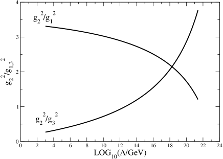
Figure 1: The ratio of $g_{2}^{2}/g_{1}^{2}$ (upper line) and $g_{2}^{2}/g_{3}^{2}$ (lower line) as a function energy scale.

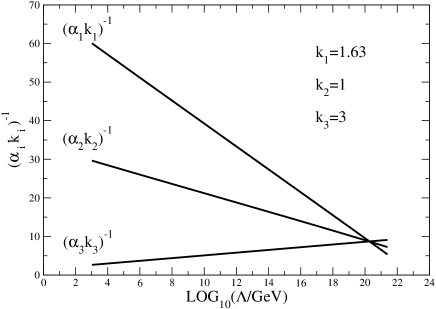
Figure 2: The running of $(\alpha_{1}k_{1})^{-1},(\alpha_{2}k_{2})^{-1},(\alpha_{3}k_{3})^{-1}$ with $k_{3}=3,k_{2}=1$ and $k_{1}\simeq 1.63$. The unification scale is $10^{20}$ GeV.

In this example the gauge couplings do not exactly satisfy the unification conditions (10) at $M_{PL}$, but it is suggesting a right direction. If we take into account the threshold corrections at $M_{PL}$, for instance, the conditions could be exactly satisfied.

Our study shows that it is certainly worthwhile to look at the other models more in detail.

Acknowledgement

The Summer Institute 2006 is sponsored by the Asia Pacific Center for Theoretical Physics and the BK 21 program of the Department of Physics, KAIST. The author would like to thank the organizers of Summer Institute 2006.

References

- [1] K. Fujikawa, Phys. Rev. Lett. 42, 1195 (1979); Phys. Rev. D21, 21 (1980); Phys. Rev. Lett. 44, 1733 (1980).
- [2] L. E. Ibáñez and G. G. Ross, Phys. Lett. B260, 291 (1991); Nucl. Phys. B368, 3 (1992); L. E. Ibáñez, Nucl. Phys. B398, 301 (1993); T. Banks, M. Dine, Phys. Rev. D45, 1424 (1992).
- [3] K. S. Babu, I. Gogoladze and K. Wang, Nucl. Phys. B660, 332 (2003).
- [4] K. Kurosawa, N. Maru and T. Yanagida, Phys. Lett. B512, 203 (2001); J. Kubo and D. Suematsu, Phys. Rev. D64, 115014 (2001).
- [5] H. K. Dreiner, C. Luhn, H. Maruyama and M. Thormeier, hep-ph/0610026; H. K. Dreiner, C. Luhn and M. Thormeier, Phys. Rev. D73, 075007 (2005).
- [6] M. B. Green and J. H. Schwarz, Phys. Lett. B149, 117 (1984); Nucl. Phys. B255, 93 (1985); M. B. Green, J. H. Schwarz and P. West, ibid. B254, 327 (1985).
- [7] K. Konishi and K. Shizuya, Nuovo. Cim. A90, 111 (1985).
- [8] E. Ma and G. Rajasekaran, Phys. Rev. D64, 113012 (2001); E. Ma, Mod. Phys. Lett. A17, 627 (2002); K. S. Babu, E. Ma and J. W. F. Valle, Phys. Lett. B552, 207 (2003); J. Kubo, A. Mondragón, M. Mondragón and E. Rodríguez-Jáuregui, Prog. Theor. Phys. 109, 795 (2003); J. Kubo, Phys. Lett. B578, 156 (2005); W. Grimus and L. Lavoura, Phys. Lett. B572, 189 (2003); W. Grimus, A. S. Joshipura, S. Kaneko, L. Lavoura and M. Tanimoto, JHEP. 0407, 078 (2004); S. L. Chen and E. Ma, Phys. Lett. B620, 151 (2005); E. Ma, Fizika, B14, 35 (2005); G. Altarelli and F. Feruglio, Nucl. Phys. B741, 215 (2006); C. Hagedorn, M. Lindner and R. N. Mohapatra, JHEP. 0606, 042 (2006); C. Hagedorn, M. Lindner and F. Plentinger, Phys. Rev. D74, 025007 (2006), and references therein.
- [9] K. S. Babu and J. Kubo, Phys. Rev. D71, 056006 (2005).