The Pomeranchuk Singularity and Vector Boson Reggeization in Electroweak Theory
J. Bartels^a, L. N. Lipatov${}^{a\dagger\;b}$, K. Peters^c
a II. Institut für Theoretische Physik, Universität Hamburg
Luruper Chaussee 149, D-22761 Hamburg, Germany
^bPetersburg Nuclear Physics Institute
Gatchina, 188 300 St.Petersburg, Russia
^c School of Physics & Astronomy, University of Manchester,
Manchester M13 9PL, UK

Abstract

We investigate the high energy behaviour of vector boson scattering in the electroweak sector of the standard model. In analogy with the BFKL analysis in QCD we compute production amplitudes in the multi-Regge limit and derive, for the vacuum exchange channel, the integral equation for vector particle scattering. We also derive and solve the bootstrap equations for the isospin-$1$ exchange channel, both for the reggeizing charged and non-reggeizing neutral vector bosons.

 

^(†) Marie Curie Chair of Excellence.
Work supported in part by the grant RFBR-04-02-17513.

1 Introduction

One of the topics to be examined in a future high energy electron positron collider is the scattering of electroweak vector bosons. Historically it was the high energy behaviour of these scattering processes which has led to the requirement of introducing a scalar Higgs boson; a closer look at the unitarity properties puts bounds on the masses of the Higgs particle. With the possibility of performing, at the linear collider, precision experiments of electroweak processes, it will be necessary to consider electroweak higher order corrections; vector boson scattering is an important class of processes to be studied with high accuracy.

Unitarity properties of vector scattering reactions are most stringent near the forward direction where cross sections are large. The object of central interest is the total cross section, i.e. the nature of the Pomeranchuk singularity. Related to this is the question whether the fields of the electroweak sector, in particular the gauge bosons of the broken gauge group, reggeize; the property of reggeization provides an indication of a possible compositenes. It is well known that the gauge bosons of nonabelian gauge theories reggeize in the leading logarithmic approximation (LLA)  [1, 2, 3, 4]; this includes both unbroken gauge symmetries (e.g. QCD) and spontaneously broken models, such as the (pure) $SU(2)$ Higgs model. On the other hand, the gauge boson of the abelian theory of QED seems to be elementary (i.e. non-reggeizing), at least on that level of accuracy which has been investigated so far. As to the case of the broken $SU(2)\times U(1)$, the charged vector bosons lie on Regge trajectories, whereas the situation of the neutral sector is more complicated: several years ago  [5, 6] strong arguments have been given that there exists a neutral Regge pole, but neither the photon nor the $Z$ boson lie on this trajectory.

The best way of exploring the vacuum exchange channel and the reggeization in the electroweak sector is by following the calculation of the BFKL Pomeron in QCD: beginning with the production amplitudes in the multi-Regge region one derives integral equations which, in the vacuum exchange channel, describe the elastic scattering and the total cross section, and, in the isospin-one channel, the reggeization of the vector particles. In this paper we describe such an analysis of the electroweak sector of the standard model. As our main results, we present the integral equation for the scattering amplitude for the vacuum exchange (‘electroweak Pomeron’), and we construct bootstrap equations to investigate the reggeization in both the charged and neutral vector bosons exchange channels.

This paper is organized as follows. In the following section 2 we define the setup of our calculations, and we collect the lowest order results of vector-vector scattering. In section 3 we compute, in the Born approximation, production amplitudes in the multi-Regge limit. Section 4 contains one and two loop results. In section 5 we write down the integral equations, and we discuss the solutions, both for the isospin one exchange channel and for the vacuum channel. In the following section we describe, as an application of our integral equations, the two-loop approximation for elastic $WW$ scattering. Concluding remarks are contained in a final section.

2 Setup and Lowest Order Electroweak Amplitudes

In this section we define the setup of our calculations, and we collect the results for vector scattering in the Born approximation. Since we will be interested on the leading-logarithmic approximation (LLA), we will neglect fermions. Let us begin with the simple model, in which the Weinberg angle $\vartheta_{W}$ is zero. In this case, the $U(1)$ gauge boson, the $B$-boson, is a free massless particle, and the $W$-bosons are described by the isovector field $\overrightarrow{W}_{\mu}$ with mass $M$. The $B$ boson decouples from the $W$ bosons, and we are dealing with a spontaneously broken $SU(2)$ models. The polarization vectors $e_{\mu}^{\lambda}$ of the $W$ bosons in the physical gauge are

$$e_{\mu}^{1,2}=e_{\mu\perp}^{1,2}\,,\,\,e_{\mu}^{3}\simeq\frac{k_{0}}{M}\delta_{\mu 3}\,+\frac{k_{3}}{M}\delta_{\mu 0}\,,\,\,k_{\mu}\,e_{\mu}^{\lambda}=0\,,\,\,(e_{\mu}^{\lambda})^{2}=-1\,,$$ (1)

where $k=(k_{0},k_{3},0,0)$ is the momentum of the vector boson moving along the third axis. There is also the Higgs particle with the mass $M_{h}$. We use Sudakov variables:

$$k=\alpha p_{A}+\beta p_{B}+k_{\perp}\,\,,k_{\perp}^{2}=-\mbox{\boldmath$k$}^{2},$$ (2)

where $p_{A}$ and $p_{B}$ are two light-like vectors along the 3-direction. In Regge kinematics we have

$$s=(p_{A}+p_{B})^{2}=(2E)^{2}\,\gg-t=-(p_{A^{\prime}}-p_{A})^{2}=\overrightarrow{q}^{2}\sim M^{2}\,.$$ (3)

The Born amplitude for the high energy scattering $A+B\rightarrow A^{\prime}+B^{\prime}$ of the $W$-bosons having definite polarizations $\lambda_{r}$ ($r=A,B,A^{\prime},B^{\prime}$) is (see Ref. [2])

$$A_{AB}^{(0)A^{\prime}B^{\prime}}=2s\,\,g\,a_{\lambda_{A}}\delta_{\lambda_{A},\lambda_{A^{\prime}}}T_{A^{\prime}A}^{c}\,\frac{1}{t-M^{2}}\,g\,a_{\lambda_{B}}\delta_{\lambda_{B},\lambda_{B^{\prime}}}T_{B^{\prime}B}^{c}\,$$ (4)

with

$$a_{1,2}=-1\,,\,\,a_{3}=-\frac{1}{2}\,.$$ (5)

For the production of a Higgs particle in $W$-boson collisions the amplitude also has the factorized form

$$A_{AB}^{(0)hB^{\prime}}=2s\,\,g\,a_{3}\delta_{\lambda_{A},3}\,\delta_{cA}\,\frac{1}{t-M^{2}}\,g\,a_{\lambda_{B}}\delta_{\lambda_{B},\lambda_{B^{\prime}}}T_{B^{\prime}B}^{c}\,.$$ (6)

The isospin generators $T_{A^{\prime}A}^{c}\,$ in the above expressions belong to the adjoint representation of the $SU(2)$-group: $T_{A^{\prime}A}^{c}=-i\varepsilon_{cA^{\prime}A}$.

When generalizing, within the leading logarithmic approximation (LLA)

$$g^{2}\ln\,\frac{s}{M^{2}}\,\sim 1\,,\,\,g^{2}\sim 1\,,$$ (7)

the Born amplitudes to higher order, it is known that the $W$ bosons reggeize, and (4) takes the form:

$$A^{LLA}=A^{(0)}\,\frac{1}{2}\left(\left(\frac{s}{M^{2}}\right)^{\omega(t)}+\left(-\frac{s}{M^{2}}\right)^{\omega(t)}\right)\,\sim A^{(0)}\left(\frac{s}{M^{2}}\right)^{\omega(t)},$$ (8)

where $\alpha_{w}(t)=1+\omega_{w}(t)$ is the $W$ boson Regge trajectory, and

$$\omega_{w}(t)=(t-M^{2})\beta(\mbox{\boldmath$q$}^{2})\,,\,\,\,\beta(\mbox{\boldmath$q$}^{2})=g^{2}\int\frac{d^{2}k}{(2\pi)^{3}}\,\frac{1}{\left(\mbox{\boldmath$k$}^{2}+M^{2}\right)\left((\mbox{\boldmath$q$}-\mbox{\boldmath$k$})^{2}+M^{2}\right)}\,,\,\,t=-\mbox{\boldmath$q$}^{2}.$$ (9)

Let us now turn to the unified model of electroweak interactions. Starting from the nondiagonal mass matrix of the fields $W^{(3)}$ and $B$

$$M^{2}\left(W^{(3)},B\right)\left(\begin{array}[]{cc}1&-\tan\,\vartheta_{w}\\ -\tan\,\vartheta_{w}&\tan^{2}\,\vartheta_{w}\end{array}\right)\left(\begin{array}[]{c}W^{(3)}\\ B\end{array}\right)\,,$$ (10)

we introduce their linear combinations corresponding to the $Z$ boson and photon:

$$Z = c_{w}W^{(3)}-s_{w}B$$

$$A = s_{w}W^{(3)}+c_{w}B\,,$$ (11)

where

$$\tan\,\vartheta_{w}=\frac{g^{\prime}}{g}\;\;,c_{w}=\cos\,\vartheta_{w}\;\;,s_{w}=\sin\vartheta_{w}.$$ (12)

In the new basis, the mass matrix becomes diagonal with the eigenvalues

$$M_{Z}^{2}=\frac{M^{2}}{c_{w}^{2}}\,,\;\;\;M_{\gamma}^{2}=0\,.$$ (13)

In the following we will put $M_{W}=M$ and $W^{(\pm)}=\frac{1}{\sqrt{2}}\left(W^{(1)}\mp iW^{(2)}\right)$.

With these definitions we generalize our previous results of the $SU(2)$ spontaneously broken gauge theory to the Weinberg-Salam model. Starting from the ($W^{(3)},B$) basis, the propagator of the neutral bosons can be written in the following operator form:

$$D_{\mu\nu}(k)=\left(\begin{array}[]{c}c_{w}\\ -s_{w}\end{array}\right)\frac{\delta_{\mu\nu}-\frac{k_{\mu}k_{\nu}}{M_{z}^{2}}}{k^{2}-M_{z}^{2}}\left(\begin{array}[]{cc}c_{w}\,,&-s_{w}\end{array}\right)$$

$$+\left(\begin{array}[]{c}s_{w}\\ c_{w}\end{array}\right)\frac{\delta_{\mu\nu}}{k^{2}}\left(\begin{array}[]{cc}s_{w}\,,&c_{w}\end{array}\right),$$ (14)

where we have used the physical gauge for the $Z$-boson and the Feynman gauge for the photon.

The linearized interaction of these vector bosons with the Higgs field $\varphi$, in the $(W^{(3)},B)$-representation, contains the matrix

$$g\,M\,\left(\begin{array}[]{cc}1&-\tan\,\vartheta_{w}\\ -\tan\,\vartheta_{w}&\tan^{2}\,\vartheta_{w}\end{array}\right),$$ (15)

proportional to the mass matrix (10). In the $(Z,A)$-representation this matrix becomes diagonal with only one non-zero coupling constant, $gM_{z}^{2}/M_{W}$, for the $ZZ\varphi$-interaction.

As to the other interaction terms, we first note that, when working in the leading $\ln s$ approximation, and restricting ourselves to scattering processes of vector bosons and Higgs particles, we can disregard the fermions. As a result, in the $(W^{(3)},B)$-representation, the $U(1)$ gauge boson, $B$, decouples and only the $W^{(3)}$-boson enters in the Yang-Mills action (together with $W^{(\pm)}$-bosons). Therefore, all gauge boson interaction terms that are needed for our discussion are obtained by starting from the $SU(2)$ part of the Yang-Mills action and substituting

$$W^{(3)}=c_{w}Z+s_{w}A\,.$$ (16)

We now turn to the $2\to 2$ scattering amplitudes, eqs.(4), (6). For the vector exchange propagators we replace

$$\frac{1}{\mbox{\boldmath$q$}^{2}+M^{2}}\rightarrow\frac{c_{w}^{2}}{\mbox{\boldmath$q$}^{2}+M_{Z}^{2}}\;,\;\;\;\frac{s_{w}^{2}}{\mbox{\boldmath$q$}^{2}}\,.$$ (17)

for $Z$ and $\gamma$ exchanges, respectively. For the helicity conserving couplings, $a_{\lambda}$ , we have to observe that the masses of external and exchanged vector bosons can be different from each other. Therefore, repeating and generalizing the algebra outlined in Ref. [2] one finds for the helicity factor of longitudinally vector bosons:

Figure 1: Mass assignment in the reggeon - particle - particle vertex

$$a_{3}^{i;jk}=\frac{M_{i}^{2}-M_{j}^{2}-M_{k}^{2}}{2M_{j}M_{k}}\,,$$ (18)

where the labels $i,j,k$ refer to exchanged, outgoing vector, and incoming particle, respectively (Fig.1). For the transverse polarization the helicity factors $a_{\lambda}$ remain the same as in the pure $SU(2)$ case. As before, each helicity factor $a_{\lambda}$ is multiplied by a helicity conserving Kronecker $\delta$-function, e.g. $\delta_{\lambda_{A},\lambda_{A^{\prime}}}$. Using the labels $W$, $\gamma$, $Z$, $W_{3}$, we define new helicity factors $a_{\lambda}^{i;jk}$, which include, in addition to the pure helicity part in eq.(18), also the Kronecker delta functions and the isospin factors, $T^{c}_{A^{\prime}A}=-i\epsilon_{cA^{\prime}A}$. In the basis of the charged $W$ bosons, we have $T^{W_{3}}_{W^{(+)}W^{(-)}}=-T^{W_{3}}_{W^{(-)}W^{(+)}}=+1$ (in the lower indices, the first one refers to the final state, the second one to the initial state; we count all particles as incoming); each permutation or charge conjugation introduces a change in sign. Finally, we have to include the coefficients $c_{w}$, $s_{w}$ from (16). We summarize the results for these reggeon-particle-particle couplings in Table 1 (we still use the same letter $a_{\lambda}^{i;jk}$ as in (18)). Here we have listed only those configurations for which the isospin factors are $+1$. The other configurations can be obtained by observing the antisymmetry of the isospin factors; for example,

$$a_{\lambda}^{Z;W^{(-)}W^{(+)}}=-a_{\lambda}^{Z;W^{(+)}W^{(-)}},\;\;a_{\lambda}^{W^{(-)};ZW^{(+)}}=-a_{\lambda}^{W^{(-)};W^{(+)}Z}\,.$$ (19)

Note that, for the $Z$-boson and for the photon, the $t$-channel propagators include additional factors (see (17)).

$$\begin{array}[]{|c|c|c|c|c|c|}\hline\cr&a_{\lambda}^{W^{(-)};ZW^{(+)}}&a_{\lambda}^{W^{(-)};\gamma W^{(+)}}&a_{\lambda}^{Z;W^{(+)}W^{(-)}}&a_{\lambda}^{\gamma;W^{(+)}W^{(-)}}&a_{\lambda}^{W_{3};W^{(+)}W^{(-)}}\\ \hline\cr\lambda=1,2&-c_{w}&-s_{w}&-1&-1&-1\\ \hline\cr\lambda=3&-\frac{1}{2}&0&-1+\frac{1}{2c_{w}^{2}}&-1&-\frac{1}{2}\\ \hline\cr\end{array}$$

$$\begin{array}[]{|c|c|c|c|c|}\hline\cr&a_{\lambda}^{W;HW}&a_{\lambda}^{Z;HZ}&a_{\lambda}^{\gamma;H\gamma}&a_{\lambda}^{W_{3};HZ}\\ \hline\cr\lambda=1,2&0&0&0&0\\ \hline\cr\lambda=3&-\frac{1}{2}&-\frac{1}{2c_{w}^{2}}&0&-\frac{1}{2}\\ \hline\cr\end{array}$$

Table 1: reggeon - particle - particle couplings

As a result, the $2\to 2$ Born amplitude for the process $ii^{\prime}\to kk^{\prime}$ with the exchange of boson $j$ has the general form:

$$A^{(0)}=2sga_{\lambda_{i}}^{j;i^{\prime}i}\frac{1}{-\mbox{\boldmath$q$}^{2}-M_{j}^{2}}ga_{\lambda_{i^{\prime}}}^{j;k^{\prime}k}\,,$$ (20)

with the substitution (17) for $Z$ and $\gamma$ exchanges, and the couplings $a_{\lambda_{A}}^{i;jk}$ have to be read off from the table. This completes the generalization of eqs.(4) and (6) to the Weinberg-Salam model.

A final remark on expression (8). In the pure $SU(2)$ case we know that the $W$ bosons reggeize, which means that the form (8) is valid. For the Weinberg-Salam theory, however, we have to find which of the bosons reggeize. It will turn out that in the neutral channel neither the $Z$-boson nor the photon lie on Regge trajectories (see also Refs.  [5, 6]). As a result, the simple expression (8) is valid only for the exchange of charged vector mesons, but not for the neutral vector exchange.

It will be useful to introduce a convenient diagrammatic notation. Since neutral and charged vector bosons are behaving quite differently, it will be helpful to distinguish between them: solid lines will be used to denote the charged $W$-boson propagators, and wavy lines stand for the neutral particle propagators (note, however, that only the $Z$ part of the corresponding matrix (15) couples to the Higgs boson). Examples are given in Fig.2.

Figure 2: Two body scattering processes (black lines denote charged bosons, wavy lines stand for neutral bosons): (a) $ZZ\to W^{(+)}W^{(-)}$; (b) $W^{(+)}W^{(-)}\to W^{(+)}W^{(-)}$.

3 Production Amplitudes

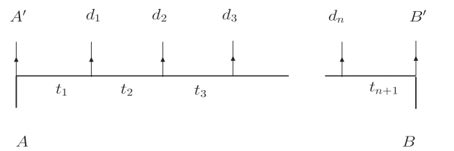
Figure 3: Production process $A+B\to A^{\prime}+d_{1}+d_{2}...+d_{n}+B^{\prime}$

Let us now consider production amplitudes $A+B\rightarrow A^{\prime}+B^{\prime}+d_{1}+d_{2}+...+d_{n}$ (where $k_{0}=p_{A^{\prime}},\,k_{n+1}=p_{B^{\prime}}$) in the multiregge region:

$$s\gg s_{i}=(k_{i-1}+k_{i})^{2}\gg\mbox{\boldmath$q$}_{r}^{2}=\left(\mbox{\boldmath$p$}_{A}-\sum_{i=0}^{r-1}\mbox{\boldmath$k$}_{i}\right)^{2}\sim M^{2}\sim M_{h}^{2}\,.$$ (21)

We again begin with the pure $SU(2)$ case. In the Born approximation the production amplitude equals:

$$A_{AB}^{(0)\;A^{\prime}B^{\prime}d_{1}...d_{n}}=$$

$$2s\,\,g\,a_{\lambda_{A}}\delta_{\lambda_{A},\lambda_{A^{\prime}}}T_{A^{\prime}A}^{c_{1}}\,\frac{1}{-\mbox{\boldmath$q$}_{1}^{2}-M^{2}}\;\,gT_{c_{2}c_{1}}^{d_{1}}C_{\mu_{1}}(q_{2},q_{1})e^{\mu_{1}}(k_{1})\frac{1}{-\mbox{\boldmath$q$}_{2}^{2}-M^{2}}...g\,a_{\lambda_{B}}\delta_{\lambda_{B},\lambda_{B^{\prime}}}T_{B^{\prime}B}^{c_{n+1}}\,,$$ (22)

where the effective vertex $C_{\mu}(q_{r+1},q_{r})\,,\,\,k_{r}=q_{r}-q_{r+1}$ for $r=1$ is given by:

$$C(q_{2},q_{1})=-q_{1\;\perp}-q_{2\;\perp}-p_{A}\left(\frac{\mbox{\boldmath$q$}_{1}^{2}+M^{2}}{k_{1}p_{A}}-\frac{k_{1}p_{B}}{p_{A}p_{B}}\right)+p_{B}\left(\frac{\mbox{\boldmath$q$}_{2}^{2}+M^{2}}{k_{1}p_{B}}-\frac{k_{1}p_{A}}{p_{A}p_{B}}\right).$$ (23)

It has the simple Ward identity property

$$k_{1}^{\mu}C_{\mu}(q_{2},q_{1})=0\,,$$ (24)

where $k_{1}=q_{1}-q_{2}$, and we have used the reality condition

$$\frac{2\,k_{1}p_{A}\,2\,k_{1}p_{B}}{s}=\mbox{\boldmath$k$}_{1}^{2}+M^{2}$$ (25)

for the produced particle.

In the case where, instead of a $W$-boson with the momentum $k_{r}$, a Higgs particle with the momentum $k_{r}$ is produced, we substitute

$$C_{\mu_{r}}(q_{r+1},q_{r})\,e^{\mu_{r}}(k_{r})\,T_{c_{r+1}c_{r}}^{d_{r}}\rightarrow M\,\delta_{c_{r+1}c_{r}}\,.$$ (26)

When in LLA higher order corrections are taken into account, the production amplitude, in the pure $SU(2)$ case, has the multi-Regge form (neglecting signature factors):

$$A_{2\rightarrow 2+n}^{LLA}=A_{2\rightarrow 2+n}^{(0)}\,\left(\frac{s_{1}}{M^{2}}\right)^{\omega(t_{1})}\left(\frac{s_{2}}{M^{2}}\right)^{\omega(t_{2})}...\left(\frac{s_{n+1}}{M^{2}}\right)^{\omega(t_{n+1})}\,,\,\,\,s_{r}=2k_{r-1}k_{r}\,,\,\,t_{r}=-\mbox{\boldmath$q$}_{r}^{2}\,.$$ (27)

(as we will see below, for the Weinberg-Salam model the generalization of the Born amplitude will be slightly more complicated). To apply the $s$-channel unitarity one needs to know the product of two effective vertices $C_{\mu}$. Using the mass shell condition (25) we obtain:

$$C_{\mu}(q_{2},q_{1})\,C^{\mu}(q-q_{2},q-q_{1})=\hskip 256.0748pt$$

$$2\;\;\frac{(\mbox{\boldmath$q$}_{1}^{2}+M^{2})((\mbox{\boldmath$q$}-\mbox{\boldmath$q$}_{2})^{2}+M^{2})+(\mbox{\boldmath$q$}_{2}^{2}+M^{2})((\mbox{\boldmath$q$}-\mbox{\boldmath$q$}_{1})^{2}+M^{2})}{(\mbox{\boldmath$q$}_{1}-\mbox{\boldmath$q$}_{2})^{2}+M^{2}}-2\;\mbox{\boldmath$q$}^{2}-3\;M^{2}\,.$$ (28)

One should also calculate the product of two isospin matrices. We decompose them in terms of various isospin structures in the $t$-channel:

$$\varepsilon_{ABd\,}\,\,\varepsilon_{A^{\prime}B^{\prime}d}=\sum_{T=0,1,2}r^{(T)}P_{AB}^{A^{\prime}B^{\prime}}(T),\;\;\;r^{(0,1,2)}=(2,1,-1)\,.$$ (29)

Here $P_{AB}^{A^{\prime}B^{\prime}}(T)$ are the projectors to the isospin states with $T=0,1,2$:

$$P_{AB}^{A^{\prime}B^{\prime}}(0) = \frac{1}{3}\delta_{AA^{\prime}\,}\delta_{BB^{\prime}\,},$$

$$P_{AB}^{A^{\prime}B^{\prime}}(1) = \frac{1}{2}\varepsilon_{cA^{\prime}A\,}\varepsilon_{cB^{\prime}B\,},$$

$$P_{AB}^{A^{\prime}B^{\prime}}(2) = \frac{1}{2}\left(\delta_{AB}\,\delta_{A^{\prime}B^{\prime}\,}+\delta_{AB^{\prime}\,}\delta_{A^{\prime}B\,}\right)-\frac{1}{3}\delta_{AA^{\prime}\,}\delta_{BB^{\prime}\,}.$$ (30)

Let us now turn to the realistic Weinberg-Salam model. The main task is the generalization of the effective production vertex (23) to the case where the attached $t$-channel bosons have different masses ($M_{W}$ for the $W$ boson, $M_{Z}$ for the $Z$ boson, or zero mass for the photon). Again, it is needed to return to Ref.  [2] for computing the $2\to 3$ production amplitudes in the double Regge limit. The result of this analysis which will not be presented in detail is that the Born approximation is still of the factorized form (22), where the couplings to the incoming particles, $a_{\lambda}^{i;jk}$, are the same as in Table 1. In the crossing channels we have the propagators $1/(-\mbox{\boldmath$q$}_{i}^{2}-M_{i}^{2})$. If we denote the masses of the exchanged vector particle on the right (left) hand side of a produced vector boson with mass $M$ by $M_{2}$ ($M_{1}$), the effective production vertex becomes

$$C(q_{2},q_{1})^{M;M_{2}M_{1}}=-q_{1\;\perp}-q_{2\;\perp}-p_{A}\left(\frac{\mbox{\boldmath$q$}_{1}^{2}+M_{1}^{2}}{k_{1}p_{A}}-\frac{k_{1}p_{B}}{p_{A}p_{B}}\right)+p_{B}\left(\frac{\mbox{\boldmath$q$}_{2}^{2}+M_{2}^{2}}{k_{1}p_{B}}-\frac{k_{1}p_{A}}{p_{A}p_{B}}\right)$$ (31)

(note that the dependence upon $M$ is through eq.(25)). If the produced vector particle is a $Z$ boson (photon), an additional factor $c_{w}$ ($s_{w}$) has to be included. Finally, each exchanged $Z$ boson receives, in the numerator, a factor $c_{w}^{2}$, each photon propagator a factor $s_{w}^{2}$ (see (17)). For the Higgs production we can use (26), where on the rhs $M$ becomes $M_{W}$, if the Higgs is produced from $W^{(\pm)}$ exchange. For Higgs production from a $Z$ exchange, replace $M\to M_{W}/c_{w}^{4}$ (and retain the factor $c_{w}^{2}$ for each $Z$ exchange propagator). Finally, in (27) the group factors $T^{d_{1}}_{c_{2}c_{1}}$ have to be rewritten in terms of $Z$ and $W^{(\pm)}$ (cf. the discussion before (19); note that both the $Z$ and the photon couple to the third component of the isospin generator: $T^{Z}_{c_{2}c_{1}}=T^{\gamma}_{c_{2}c_{1}}=T^{3}_{c_{2}c_{1}}$).

The Ward identity (24) for the production vertex is replaced now by the relation

$$k_{1}^{\mu}C_{\mu}^{M;M_{2}M_{1}}(q_{2},q_{1})=M_{2}^{2}-M_{1}^{2}\,.$$ (32)

For the $s$-channel unitarity integration we again need the product of two effective vertices. More precisely, one should sum over the physical helicities of the produced boson with mass $M_{m}$:

$$\sum_{\lambda}\epsilon_{\lambda}^{\mu}(k_{1})\epsilon_{\lambda}^{\nu}(k_{1})=-g^{\mu\nu}+\frac{k_{1}^{\mu}k_{1}^{\nu}}{M_{m}^{2}}$$ (33)

(note that for the production of a photon with $M_{m}=0$ the second term is absent in an accordance with the vanishing of (32) for $M_{1}=M_{2}$).

Figure 4: Assigment of masses for the product of two effective vertices

For the mass assignment illustrated in Fig.4 we obtain (cf.(3)):

$$C_{\mu}^{M_{m};M_{j}M_{i}}(q_{j},q_{i})\,(g^{\mu\nu}-\frac{k_{1}^{\mu}k_{1}^{\nu}}{M_{m}^{2}})\,C_{\nu}^{M_{m};M_{l}M_{k}}(q-q_{j},q-q_{i})=$$ (34)

$$-2\mbox{\boldmath$q$}^{2}+M_{m}^{2}-M_{i}^{2}-M_{j}^{2}-M_{k}^{2}-M_{l}^{2}+\frac{(M_{j}^{2}-M_{i}^{2})(M_{l}^{2}-M_{k}^{2})}{M_{m}^{2}}+$$

$$2\;\frac{(\mbox{\boldmath$q$}_{i}^{2}+M_{i}^{2})((\mbox{\boldmath$q$}-\mbox{\boldmath$q$}_{j})^{2}+M_{l}^{2})+((\mbox{\boldmath$q$}-\mbox{\boldmath$q$}_{i})^{2}+M_{j}^{2})(\mbox{\boldmath$q$}_{j}^{2}+M_{k}^{2})}{(\mbox{\boldmath$q$}_{i}-\mbox{\boldmath$q$}_{j})^{2}+M_{m}^{2}}\,.$$

This result can be obtained with the use of eqs.(25) (31), and (32).

4 One and two loop results

$2\to 2$ scattering in one loop

We are now ready to carry out the BFKL program. Beginning with one loop amplitudes, we first consider the charged isospin-1 exchange. To be definite, let us study the process $ZZ\to W^{(+)}W^{(-)}$.

Figure 5: One loop corrections to $2\to 2$ – processes shown in Fig.2

The Born diagram is shown in Fig.2a, the first corrections come from the box diagrams of the type Fig.5a-d. For the energy discontinuities we use the unitarity conditions, e.g.

$${\rm Im_{s}}\,A^{(1)}_{ab\to a^{\prime}b^{\prime}}=\frac{1}{2}\sum_{i}\int d\Pi_{2}A^{(0)}_{ab\to i}(k^{2})A^{(0)\dagger}_{i\to a^{\prime}b^{\prime}}((k-q)^{2})\,,$$ (35)

where the sum in $i$ extends over all possible intermediate two-particle states, and we then make use of dispersion relations to compute the scattering amplitudes. We define the functions $\beta_{ij}(q^{2})$:

$$\beta_{ij}(q^{2})=g^{2}\int\frac{d^{2}k}{(2\pi)^{3}}\frac{1}{\mbox{\boldmath$k$}^{2}+M_{i}^{2}}\,\frac{1}{(\mbox{\boldmath$k$}-\mbox{\boldmath$q$})^{2}+M_{j}^{2}}\,.$$ (36)

We also use their generalizations:

$$\beta_{ijk}(q^{2})=g^{4}\int\frac{d^{2}kd^{2}k^{\prime}}{(2\pi)^{6}}\frac{1}{\mbox{\boldmath$k$}^{2}+M_{i}^{2}}\,\frac{1}{{\mbox{\boldmath$k$}^{\prime}}^{2}+M_{j}^{2}}\,\frac{1}{(\mbox{\boldmath$k$}+\mbox{\boldmath$k$}^{\prime}-\mbox{\boldmath$q$})^{2}+M_{k}^{2}}\,.$$ (37)

The subscripts indicate the type of vector particles inside the $\beta$ functions.

The Born amplitude has the form

$$A^{(0)}_{11}=2sga_{\lambda_{A}}^{W^{(+)};W^{(-)}Z}\frac{1}{-\mbox{\boldmath$q$}^{2}-M_{W}^{2}}ga_{\lambda_{B}}^{W^{(-)};W^{(+)}Z}.$$ (38)

Next we form signatured amplitudes. In our case, $ZZ\to W^{(+)}W^{(-)}$, they are defined by the combinations

$$\frac{1}{2}\left(A_{ZZ\to W^{(+)}W^{(-)}}\;\;\pm\;\;A_{W^{(-)}Z\to ZW^{(-)}}\right).$$ (39)

Signature describes the symmetry under $s\to-s$. Because of the antisymmetry properties of the isospin coefficients, the Born amplitude for our process belongs to odd signature (in terms of isospin, it is the antisymmetric $T=1$ representation, $T_{3}=\pm 1$). Using the unitarity relations for the processes $ZZ\to W^{(+)}W^{(-)}$ (Fig.5a, b) and for the cross process $W^{(-)}Z\to ZW^{(-)}$ (Fig.5c, d), we obtain for the odd-signature amplitude:

$$A^{(1)}_{11}=[s\ln(-s)-u\ln(-u)]\,ga_{\lambda_{A}}^{W^{(+)};W^{(-)}Z}\Big{\{}c_{w}^{2}\,\beta_{wz}(q^{2})+s_{w}^{2}\,\beta_{w\gamma}(q^{2})\Big{\}}ga_{\lambda_{B}}^{W^{(-)};W^{(+)}Z}\,.$$ (40)

In the LLA approximation the energy scale in the logarithm is arbitrary; it is natural to chose the scale to be of the order of $M_{W}$. We omit to explicitly write this scale.

Comparing the Born approximation with the one loop result, one is lead to interpret both expressions as being the first two terms in the power series expansion of (cf.(8))

$$A_{11}=-ga_{\lambda_{A}}^{W^{(+)};W^{(-)}Z}\frac{(-s)^{\alpha_{c}(q^{2})}-(-u)^{\alpha_{c}(q^{2})}}{-\mbox{\boldmath$q$}^{2}-M_{W}^{2}}ga_{\lambda_{B}}^{W^{(-)};W^{(+)}Z}$$ (41)

with the trajectory function

$$\alpha_{c}(q^{2})=1+(q^{2}-M_{W}^{2})\Big{[}c_{w}^{2}\,\beta_{wz}(q^{2})+s_{w}^{2}\,\beta_{w\gamma}(q^{2})\Big{]}.$$ (42)

This is consistent with the expectation that the charged $W$ bosons reggeize, in the same way as the $W$ bosons do in the pure $SU(2)$ theory. The same conclusion holds, if we replace external vector bosons by Higgs bosons. Later on we will confirm that the reggeization of the charged $W$ bosons is correct to all orders. It will be convenient to introduce

$$\omega_{c}(q^{2})=\alpha_{c}(q^{2})-1=(q^{2}-M_{W}^{2})\Big{[}c_{w}^{2}\,\beta_{wz}(q^{2})+s_{w}^{2}\,\beta_{w\gamma}(q^{2})\Big{]}.$$ (43)

Turning next to the neutral exchange, we consider the elastic scattering of two charged bosons, the process $W^{(+)}W^{(-)}\to W^{(+)}W^{(-)}$. The Born diagram is shown in Fig.2b; the amplitude has the form:

$$A^{(0)}_{10}=2s\left(ga_{\lambda_{A}}^{Z;W^{(-)}W^{(+)}}\frac{c_{w}^{2}}{-\mbox{\boldmath$q$}^{2}-M_{Z}^{2}}ga_{\lambda_{B}}^{Z;W^{(+)}W^{(-)}}+ga_{\lambda_{A}}^{\gamma;W^{(-)}W^{(+)}}\frac{s_{w}^{2}}{-\mbox{\boldmath$q$}^{2}}ga_{\lambda_{B}}^{\gamma;W^{(+)}W^{(-)}}\right).$$ (44)

It belongs to odd-signature (the $T=1$ representation), and it represents the neutral, $T_{3}=0$, component. For the one-loop odd-signature contribution we obtain (Figs.5e - f):

$$A^{(1)}_{10}=[s\ln(-s)-u\ln(-u)]\,ga_{\lambda_{A}}^{W_{3};W^{(-)}W^{(+)}}\;\beta_{ww}(q^{2})\>ga_{\lambda_{B}}^{W_{3};W^{(+)}W^{(-)}}.$$ (45)

An analogous result is obtained for the process $ZW^{(-)}\to HW^{(-)}$, with the substitution $a_{\lambda_{A}}^{W_{3};W^{(-)}W^{(+)}}\to a_{\lambda_{A}}^{W_{3};HZ}$. At this stage, it seems premature to draw any conclusion about the connection of the one loop result with the Born approximation.

The one-loop even signature contribution of Fig.5g contributes to both isospin 0 and 2. We present the sum of both:

$$A^{(1)}_{even}=2i\pi s\left(-\frac{1}{2}ga_{\lambda_{A}}^{W_{3};W^{(-)}W^{(+)}}\;\beta_{ww}(q^{2})\;ga_{\lambda_{B}}^{W_{3};W^{(+)}W^{(-)}}\hskip 170.71652pt\right.$$

$$\left.+\;g(a_{\lambda_{A}}^{Z;W^{(-)}W^{(+)}})^{2}\;c_{w}^{4}\;\beta_{zz}(q^{2})\;g(a_{\lambda_{B}}^{Z;W^{(+)}W^{(-)}})^{2}+\;g(a_{\lambda_{A}}^{\gamma;W^{(-)}W^{(+)}})^{2}\;s_{w}^{4}\;\beta_{\gamma\gamma}(q^{2})\;g(a_{\lambda_{B}}^{\gamma;W^{(+)}W^{(-)}})^{2}\right.$$

$$\left.+\;2\;ga_{\lambda_{A}}^{Z;W^{(-)}W^{(+)}}a_{\lambda_{A}}^{\gamma;W^{(-)}W^{(+)}}\;c_{w}^{2}s_{w}^{2}\;\beta_{\gamma z}(q^{2})\;ga_{\lambda_{B}}^{Z;W^{(+)}W^{(-)}}a_{\lambda_{B}}^{\gamma;W^{(+)}W^{(-)}}\right)\,.\hskip 42.67912pt$$ (46)

Two loop results for $2\to 2$ scattering

Two loop corrections consist of two classes of terms, the two-particle intermediate states and the three-particle intermediate states in the $s$-channel  [2]. The former ones are obtained by inserting, into the bilinear unitarity relation, the Born term on one side and one loop amplitudes on the other side. For the calculation of the three particle state we make use of expression (34); we also include the production of Higgs scalars. Let us begin with the charge exchange channel. Making use of the vertices in Table 1 and of the one-loop results listed above, and summing over all 2-particle intermediate states, we obtain for the process $ZZ\to W^{(+)}W^{(-)}$:

$$-2s\ln^{2}s\,ga_{\lambda_{A}}^{W^{(+)};W^{(-)}Z}\left(\beta_{www}(\mbox{\boldmath$q$}^{2})+c_{w}^{4}\beta_{wzz}(\mbox{\boldmath$q$}^{2})+2c_{w}^{2}s_{w}^{2}\beta_{wz\gamma}(\mbox{\boldmath$q$}^{2})+s_{w}^{4}\beta_{w\gamma\gamma}(\mbox{\boldmath$q$}^{2})\right)ga_{\lambda_{B}}^{W^{(-)};W^{(+)}Z}\,.$$ (47)

For the sum over 3-particle intermediate states we find, making use of eq.(34), a sum of two terms. The first one is:

$$(s\frac{\ln^{2}(-s)}{2!}-u\frac{\ln^{2}(-u)}{2!})ga_{\lambda_{A}}^{W^{(+)};W^{(-)}Z}\left(s_{w}^{2}\beta_{w\gamma}(\mbox{\boldmath$q$}^{2})+c_{w}^{2}\beta_{wz}(\mbox{\boldmath$q$}^{2})\right)$$

$$\left(-\mbox{\boldmath$q$}^{2}-M_{W}^{2}\right)\left(s_{w}^{2}\beta_{w\gamma}(\mbox{\boldmath$q$}^{2})+c_{w}^{2}\beta_{wz}(\mbox{\boldmath$q$}^{2})\right)ga_{\lambda_{B}}^{W^{(-)};W^{(+)}Z}.$$ (48)

The second one can be written in the form:

$$2s\ln^{2}s\,ga_{\lambda_{A}}^{W^{(+)};W^{(-)}Z}\left(\beta_{www}(\mbox{\boldmath$q$}^{2})+c_{w}^{4}\beta_{www}(\mbox{\boldmath$q$}^{2})+2c_{w}^{2}s_{w}^{2}\beta_{wz\gamma}(\mbox{\boldmath$q$}^{2})+s_{w}^{4}\beta_{w\gamma\gamma}(\mbox{\boldmath$q$}^{2})\right)ga_{\lambda_{B}}^{W^{(-)};W^{(+)}Z}\,.$$ (49)

and cancels the entire 2-particle intermediate state, eq.(47). Hence the two-loop result for the negative signature charge exchange channel coincides with the second term in the expansion of

$$-ga_{\lambda_{A}}^{W^{(+)};W^{(-)}Z}\frac{(-s)^{\alpha_{c}(q^{2})}-(-u)^{\alpha_{c}(q^{2})}}{-\mbox{\boldmath$q$}^{2}-M_{W}^{2}}ga_{\lambda_{B}}^{W^{(-)};W^{(+)}Z},$$ (50)

confirming the reggeization in the one-loop approximation.

Turning to the neutral exchange channel, we again first consider the two-particle intermediate states. For the process $W^{(+)}W^{(-)}\to W^{(+)}W^{(-)}$ we obtain, after summation over all possible 2-particle intermediate states:

$$-2s\ln^{2}s\,ga_{\lambda_{A}}^{W_{3};W^{(-)}W^{(+)}}\left(s_{w}^{2}\beta_{\gamma ww}+c_{w}^{2}\beta_{zww}\right)ga_{\lambda_{B}}^{W_{3};W^{(+)}W^{(-)}},$$ (51)

where the couplings $a_{\lambda}^{W_{3};W^{(-)}W^{(+)}}$ are listed in Table 1. The calculation of the three particle intermediate state, again, makes use of the square of the production vertex, eq.(34). Summing over all possible 3-particle intermediate states we obtain a sum of two terms. The first one is:

$$(s\frac{\ln^{2}(-s)}{2!}-u\frac{\ln^{2}(-u)}{2!})\,g\,a_{\lambda_{A}}^{W_{3};W^{(-)}W^{(+)}}\,\beta_{ww}(\mbox{\boldmath$q$}^{2})\,(-\mbox{\boldmath$q$}^{2}-M_{W}^{2})\,\beta_{ww}(\mbox{\boldmath$q$}^{2})\,g\,a_{\lambda_{B}}^{W_{3};W^{(+)}W^{(-)}},$$ (52)

the second one

$$2s\ln^{2}s\,g\,a_{\lambda_{A}}^{W_{3};W^{(-)}W^{(+)}}\left(s_{w}^{2}\beta_{\gamma ww}(\mbox{\boldmath$q$}^{2})+c_{w}^{2}\beta_{zww}(\mbox{\boldmath$q$}^{2})\right)\,g\,a_{\lambda_{B}}^{W_{3};W^{(+)}W^{(-)}}.$$ (53)

This second terms cancels against the two-particle contribution, eq.(51). We have thus only the first term, (52), which can be interpreted as the second term in the expansion of the expression

$$-ga_{\lambda_{A}}^{W_{3};W^{(-)}W^{(+)}}\frac{(-s)^{\alpha_{n}(q^{2})}-(-u)^{\alpha_{n}(q^{2})}}{-\mbox{\boldmath$q$}^{2}-M_{W}^{2}}ga_{\lambda_{B}}^{W_{3};W^{(+)}W^{(-)}}$$ (54)

with

$$\alpha_{n}(q^{2})=1+(q^{2}-M_{W}^{2})\beta_{ww}(q^{2})\,.$$ (55)

In the following we will also use the notation

$$\omega_{n}(q^{2})=\alpha_{n}(q^{2})-1=(q^{2}-M_{W}^{2})\beta_{ww}(q^{2})\,.$$ (56)

The expression (54) matches the one-loop result, (45), but it does not agree with the Born approximation, (44). We therefore make the following ansatz for the neutral exchange in the $2\to 2$ scattering process:

$$A_{10}=2s\left(ga_{\lambda_{A}}^{Z;W^{(-)}W^{(+)}}\frac{c_{w}^{2}}{-\mbox{\boldmath$q$}^{2}-M_{Z}^{2}}ga_{\lambda_{B}}^{Z;W^{(+)}W^{(-)}}+ga_{\lambda_{A}}^{\gamma;W^{(-)}W^{(+)}}\frac{s_{w}^{2}}{-\mbox{\boldmath$q$}^{2}}ga_{\lambda_{B}}^{\gamma;W^{(+)}W^{(-)}}\right)$$

$$-ga_{\lambda_{A}}^{W_{3};W^{(-)}W^{(+)}}\left(\frac{(-s)^{\alpha_{n}(q^{2})}-(-u)^{\alpha_{n}(q^{2})}}{-\mbox{\boldmath$q$}^{2}-M_{W}^{2}}+\frac{2s}{-\mbox{\boldmath$q$}^{2}-M_{W}^{2}}\right)ga_{\lambda_{B}}^{W_{3};W^{(+)}W^{(-)}},$$ (57)

i.e. we have a Regge pole in the neutral exchange channel, which passes through unity at $t=M_{W}^{2}$: neither the $Z$ boson nor the photon lie on this trajectory. Note that, in the second line of (57), the pole at $q^{2}=M_{W}^{2}$ cancels. For $s_{w}=0$, we have $M_{Z}=M_{W}$, and $\alpha_{n}$ passes through the $Z$-boson. Later on we shall verify that this result is correct to all orders.

One loop results for $2\to 3$ production amplitudes

Before we can start to write integral equations we need to calculate corrections to the production amplitudes: this will be done in the spirit of  [7]. To be definite, the process $W^{(+)}W^{(-)}\to ZZZ$ (Fig.6a)

Figure 6: $2\to 3$ production amplitudes (the dot marks the effective production vertex (eq.(31)): (a) $W^{(+)}W^{(-)}\to ZZZ$; (b) $W^{(+)}Z\to W^{(+)}W^{(+)}W^{(-)}$.

will be considered. In the Born approximation we have:

$$A_{2\to 3}^{(0)}=2sga_{\lambda_{A}}^{W^{(-)};ZW^{(+)}}\frac{1}{-\mbox{\boldmath$q$}_{1}^{2}-M_{W}^{2}}gT^{Z}_{W^{(-)}W^{(+)}}C(\mbox{\boldmath$q$}_{2},\mbox{\boldmath$q$}_{1})^{M_{Z};M_{W}M_{W}}\frac{1}{-\mbox{\boldmath$q$}_{2}^{2}-M_{W}^{2}}ga_{\lambda_{B}}^{W^{(+)};ZW^{(-)}}\,,$$ (58)

where the energy variables $s_{i}$ have been defined in (21). In order to be able to compute the discontinuity in $s_{2}$, we make a more general ansatz which exhibits the analytic structure in all three energy variables:

$$A_{2\to 3}=F_{L}s^{\alpha_{1}}s_{2}^{\alpha_{2}-\alpha_{1}}\frac{\xi_{\alpha_{1}}}{t_{1}-M_{1}^{2}}\frac{\xi_{\alpha_{2}\alpha_{1}}}{\alpha_{2}-\alpha_{1}}+F_{R}s^{\alpha_{2}}s_{1}^{\alpha_{1}-\alpha_{2}}\frac{\xi_{\alpha_{2}}}{t_{2}-M_{2}^{2}}\frac{\xi_{\alpha_{1}\alpha_{2}}}{\alpha_{1}-\alpha_{2}}\,,$$ (59)

where the signature factors are:

$$\xi_{\alpha_{1}}=e^{-i\pi\alpha_{1}}-1,$$

$$\xi_{\alpha_{1}\alpha_{2}}=e^{-i\pi(\alpha_{1}-\alpha_{2})}+1\,,$$ (60)

and $\alpha_{i}=\alpha(t_{i})$ are the corresponding Regge trajectories. The two partial waves $F_{L}$ and $F_{R}$ will be determined from the discontinuities in the $s_{2}$ and $s_{1}$ channels, resp., and we shall see that the ansatz (59) is compatible with the familiar factorized multiregge form. The discontinuity in the $s_{2}$ channel is:

$$disc_{s_{2}}A_{2\to 3}=-\pi\frac{s^{\alpha_{1}}s_{2}^{\alpha_{2}-\alpha_{1}}\xi_{\alpha_{1}}}{t_{1}-M_{1}^{2}}F_{L}\,.$$ (61)

In the lowest order, we simply put $\alpha_{i}\to 1$ and $\xi_{\alpha_{1}}\to-2$.

When computing the unitarity integral in the $s_{2}$-channel (Fig.7)

Figure 7: Unitarity integral in the $s_{2}$-subchannel.

it is convenient to first transform into the center-of-mass system of the $s_{2}$-channel, to multiply with the $2\to 2$ scattering amplitude having a simple helicity structure in the $s_{2}$ channel, to compute the two-body phase space integral, and finally to transform back into the overall cm-system. Details of this procedure have been described in  [7]; some of the formulae, however, have to be generalized to the case of unequal masses of the vector bosons. A list of the relevant expressions is presented in the appendix. After summing over all possible s-channel intermediate states and over all $t$-channel exchanges we find for the partial wave $F_{L}$:

$$F_{L}=-\frac{1}{2}sga_{\lambda_{A}}^{W^{(-)};W^{(+)}Z}\left(gT^{Z}_{W^{(-)}W^{(+)}}C(\mbox{\boldmath$q$}_{2},\mbox{\boldmath$q$}_{1})^{M_{Z};M_{W}M_{W}}\frac{\omega_{c}(q_{2}^{2})}{-\mbox{\boldmath$q$}_{2}^{2}-M_{W}^{2}}\right.$$

$$\left.-(\mbox{\boldmath$q$}_{1}^{2}+M_{W}^{2})(c_{w}^{2}K^{Z;WW}+s_{w}^{2}K^{\gamma;WW})\right)ga_{\lambda_{B}}^{W^{(+)};W^{(-)}Z}\,.$$ (62)

Here we have introduced the short-hand notation:

$$K^{Z;WW}=g^{2}T^{Z}_{W^{(-)}W^{(+)}}\int\frac{d^{2}k}{(2\pi)^{3}}\frac{gC^{M_{Z};M_{W}M_{W}}(\mbox{\boldmath$q$}_{2}-\mbox{\boldmath$k$},\mbox{\boldmath$q$}_{1}-\mbox{\boldmath$k$})}{((\mbox{\boldmath$q$}_{1}-\mbox{\boldmath$k$})^{2}+M_{W}^{2})((\mbox{\boldmath$q$}_{2}-\mbox{\boldmath$k$})^{2}+M_{W}^{2})}\frac{1}{(\mbox{\boldmath$k$}^{2}+M_{Z}^{2})}\,.$$ (63)

With an analogous result for the discontinuity in $s_{1}$ and for $F_{R}$ we return to (59). In the sum of both partial waves, the terms containing $K^{Z;WW}$ and $K^{\gamma;WW}$ cancel, and we are left with the expression

$$A_{2\to 3}=2sa_{\lambda_{A}}^{W^{(-)};W^{(+)}Z}\frac{s_{1}^{\omega_{c}(q_{1}^{2})}}{-\mbox{\boldmath$q$}_{1}^{2}-M_{W}^{2}}gT^{Z}_{W^{(-)}W^{(+)}}C(\mbox{\boldmath$q$}_{2},\mbox{\boldmath$q$}_{1})^{M_{Z};M_{W}M_{W}}\frac{s_{2}^{\omega_{c}(q_{2}^{2})}}{-\mbox{\boldmath$q$}_{2}^{2}-M_{W}^{2}}ga_{\lambda_{B}}^{W^{(+)};W^{(-)}Z},$$ (64)

i.e. the $W$ exchanges have started to reggeize. It is straightforward to verify, in lowest order, the discontinuities in $s_{1}$ and $s_{2}$ which led to the partial waves $F_{L}$ and $F_{R}$.

In an analogous way we compute the one loop corrections to other production amplitudes. For the process $W^{(+)}Z\to W^{(+)}W^{(-)}W^{(+)}$ (see Fig.6b)

Figure 8: Unitarity integrals (a) in the $s_{2}$ subchannel, (b) in the $s_{1}$ channel.

we have in the Born approximation:

$$A_{2\to 3}=2s\left(ga_{\lambda_{A}}^{Z;W^{(-)}W^{(+)}}\frac{c_{w}^{2}}{-\mbox{\boldmath$q$}_{1}^{2}-M_{Z}^{2}}gT^{W^{(+)}}_{W^{(-)}Z}C(\mbox{\boldmath$q$}_{2},\mbox{\boldmath$q$}_{1})^{M_{W};M_{W};M_{Z}}\right.$$

$$\left.+ga_{\lambda_{A}}^{\gamma;W^{(-)}W^{(+)}}\frac{s_{w}^{2}}{-\mbox{\boldmath$q$}_{1}^{2}}gT^{W^{(+)}}_{W^{(-)}\gamma}C(\mbox{\boldmath$q$}_{2},\mbox{\boldmath$q$}_{1})^{M_{W};M_{W}M_{\gamma}}\right)\cdot\;\;\frac{1}{-\mbox{\boldmath$q$}_{2}^{2}-M_{W}^{2}}ga_{\lambda_{B}}^{W^{(+)};W^{(-)}Z}.$$ (65)

For the $t_{2}$ channel we expect that, in higher orders, the $W$-exchange will reggeize. As to the $t_{1}$ channel, our analysis of the $2\to 2$ scattering process with neutral exchange, eq.(57), suggests that, in higher order, in addition to the elementary $z$ and $\gamma$ exchanges the neutral Regge pole, $\alpha_{n}$, should appear. As we have seen before, Regge pole exchanges contribute to the discontinuities in $s_{1}$ and $s_{2}$, whereas the elementary $z$ and $\gamma$ exchanges do not. Therefore, our ansatz (59) with $\alpha_{1}\to\alpha_{n}$, $\alpha_{2}\to\alpha_{c}$ should be valid for the Regge pole exchanges in both crossing channels, but we have to add extra terms for the elementary exchanges in the $t_{1}$ channel which have a discontinuity in $s_{2}$ but not in $s_{1}$, e.g. for $Z$ exchange:

$$F_{L}^{Z}ss_{2}^{\alpha_{c}-1}\frac{-2}{t_{1}-M_{Z}^{2}}\frac{\xi_{\alpha_{c}1}}{\alpha_{c}-1}\,.$$ (66)

Proceeding in the same way as before we compute, from the single discontinuities in $s_{1}$ and $s_{2}$, the partial waves $F_{L}$ and $F_{R}$ (see Fig.8). From this we infer the following all-order expression:

$$A_{2\to 3}=2s\left(ga_{\lambda_{A}}^{W_{3};W^{(-)}W^{(+)}}\frac{s_{1}^{\omega_{n}(q_{1}^{2})}-1}{-\mbox{\boldmath$q$}_{1}^{2}-M_{W}^{2}}gT^{W^{(+)}}_{W^{(-)}W_{3}}C(\mbox{\boldmath$q$}_{2},\mbox{\boldmath$q$}_{1})^{M_{W};M_{W}M_{W}}+\right.$$

$$\left.ga_{\lambda_{A}}^{Z;W^{(-)}W^{(+)}}\frac{c_{w}^{2}}{-\mbox{\boldmath$q$}_{1}^{2}-M_{Z}^{2}}gT^{W^{(+)}}_{W^{(-)}Z}C(\mbox{\boldmath$q$}_{2},\mbox{\boldmath$q$}_{1})^{M_{W};M_{W}M_{Z}}+\right.$$

$$\left.ga_{\lambda_{A}}^{\gamma;W^{(-)}W^{(+)}}\frac{s_{w}^{2}}{-\mbox{\boldmath$q$}_{1}^{2}}gT^{W^{(+)}}_{W^{(-)}\gamma}C(\mbox{\boldmath$q$}_{2},\mbox{\boldmath$q$}_{1})^{M_{W};M_{W}M_{\gamma}}\right)\cdot\;\;\frac{s_{2}^{\omega_{c}(q_{2}^{2})}}{-\mbox{\boldmath$q$}_{2}^{2}-M_{W}^{2}}ga_{\lambda_{B}}^{W^{(+)};W^{(-)}Z}.$$ (67)

In the charge exchange channel ($t_{2}$-channel) we recognize the reggeization of the $W$ boson, whereas the neutral exchange channel ($t_{1}$-channel) has the same structure as (57). In (67) the new element is the $W$ production vertex where one of the reggeons belongs to the neutral Regge pole, $\alpha_{n}$: its particle pole lies at $M_{W}$, and consequently the mass labels of the production vertex are $C(\mbox{\boldmath$q$}_{2},\mbox{\boldmath$q$}_{1})^{M_{W};M_{W}M_{W}}$.

As a final example, we calculate the production process $W^{(+)}W^{(-)}\to W^{(+)}HW^{(-)}$. Our one-loop calculation leads to:

$$A_{2\to 3}=2s\left(a_{\lambda_{A}}^{Z;W^{(-)}W^{(+)}}\frac{c_{w}^{2}}{-\mbox{\boldmath$q$}_{1}^{2}-M_{Z}^{2}}\frac{1}{c_{w}^{2}}+a_{\lambda_{A}}^{W_{3};W^{(-)}W^{(+)}}\frac{s_{1}^{\omega_{n}(q_{1}^{2})}-1}{-\mbox{\boldmath$q$}_{1}^{2}-M_{W}^{2}}\right)M_{W}$$

$$\cdot\;\;\left(\frac{1}{c_{w}^{2}}\frac{c_{w}^{2}}{-\mbox{\boldmath$q$}_{2}^{2}-M_{Z}^{2}}a_{\lambda_{B}}^{Z;W^{(+)}W^{(-)}}+\frac{s_{2}^{\omega_{n}(q_{2}^{2})}-1}{-\mbox{\boldmath$q$}_{2}^{2}-M_{W}^{2}}a_{\lambda_{B}}^{W_{3};W^{(+)}W^{(-)}}\right).$$ (68)

Note that, following our convention defined before, each $Z$ exchange carries a factor $c_{w}^{2}$. As a consequence, the production of the Higgs obtains a factor $1/c_{w}^{2}$ if, in (68), one of the attached neutral exchanges is a $Z$ boson, and a factor $1/c_{w}^{4}$ if we have a $Z$ boson on both sides of the produced Higgs. In the following we shall verify that these production amplitudes lead to the correct bootstrap equations.

5 Integral Equations

We now turn to the derivation of integral equations which represent the sum of discontinuities of the scattering amplitude over an arbitrary number of produced particles.

Figure 9: Ladder diagrams obtained from the square of production amplitudes: (a) $ZZ\to W^{(+)}W^{(-)}$ (charge exchange); (b) $W^{(+)}W^{(-)}\to W^{(+)}W^{(-)}$ (neutral exchange, odd signature).

The one and two loop calculations suggest that the $2\to n$ production amplitudes can be written in the factorized multiregge form, where charged and neutral exchanges lead to slightly different expressions. The exchange of a charged gauge boson requires the usual reggeon propagator $s_{i}^{1+\omega_{c}}/(\mbox{\boldmath$q$}^{2}+M_{W}^{2})$. For the neutral exchange we have a sum of three terms, the $Z$ and $\gamma$ exchange in the Born approximation, and the neutral Regge pole exchange. In the angular momentum representation, the corresponding propagators are

$$\frac{c_{w}^{2}}{\omega}\frac{1}{\mbox{\boldmath$q$}^{2}+M_{Z}^{2}},\hskip 28.45274pt\frac{s_{w}^{2}}{\omega}\frac{1}{\mbox{\boldmath$q$}^{2}},\hskip 28.45274pt\left(\frac{1}{\omega-\omega_{c}(q^{2})}-\frac{1}{\omega}\right)\frac{1}{\mbox{\boldmath$q$}^{2}+M_{W}^{2}}\,,$$ (69)

resp. When inserting the sum of these three terms into a production amplitude, each term comes with its own coupling to external and produced particles. For example, the couplings to an external $W$ boson are $a_{\lambda}^{Z;W^{(-)}W^{(+)}}$, $a_{\lambda}^{\gamma;W^{(-)}W^{(+)}}$, and $a_{\lambda}^{W_{3};W^{(-)}W^{(+)}}$, respectively. When, inside a multiregge production amplitude, the exchanged neutral boson couples to a $W$ production vertex, the effective production vertices are $C^{M_{W};M_{Z}M_{W}}$, $C^{M_{W};M_{\gamma}M_{W}}$, and $C^{M_{W};M_{3}M_{W}}$ with $M_{3}=M_{W}$, resp. With these rules it will be straightforward to write down the integral equations for the sum of products of production amplitudes (cf. [3])).

Let us begin with the partial wave representations. For the $2\to 2$ process with charged boson exchange we again consider the process $ZZ\to W^{(+)}W^{(-)}$ (eqs.(38) and (41)). The $t$-channel partial wave decomposition contains the Born contribution (38) and, from the Regge pole, the integral over $\omega=j-1$:

$$A_{11}(s,t)=\frac{2s}{-\mbox{\boldmath$q$}^{2}-M_{W}^{2}}ga_{\lambda_{A}}^{W^{(+)};W{(-)}Z}ga_{\lambda_{A^{\prime}}}^{W^{(-)};W{(+)}Z}\,\left(1+\int_{a-i\infty}^{a+i\infty}\frac{d\omega}{4i}s^{\omega}\frac{1+e^{-i\pi\omega}}{\pi\omega}\frac{\omega_{c}(q^{2})}{\omega-\omega_{c}(q^{2})}\right),$$ (70)

where $a>0$. We can shift the integration contour to the region $\Re\omega<0$ by cancelling the result of taking the residue of the pole at $\omega=0$ with the Born contribution:

$$A_{11}(s,t)=\frac{2s}{-\mbox{\boldmath$q$}^{2}-M_{W}^{2}}\int_{-a-i\infty}^{-a+i\infty}\frac{d\omega}{4i}\frac{1+e^{-i\pi\omega}}{\pi\omega}s^{\omega}ga_{\lambda_{A}}^{W^{(+)};W{(-)}Z}\frac{\omega_{c}(q^{2})}{\omega-\omega_{c}(q^{2})}ga_{\lambda_{A^{\prime}}}^{W^{(-)};W{(+)}Z}.$$ (71)

With the partial wave

$$F_{11}(\omega,q^{2})=\frac{\omega_{c}(q^{2})}{(\mbox{\boldmath$q$}^{2}+M_{W}^{2})(\omega-\omega_{c}(q^{2}))}$$ (72)

we write the partial wave representation in the form:

$$A_{11}(s,t)=2s\int_{-a-i\infty}^{-a+i\infty}\frac{d\omega}{4i}s^{\omega}\frac{1+e^{-i\pi\omega}}{\pi\omega}ga_{\lambda_{A}}^{W^{(+)};W{(-)}Z}F_{11}(\omega,q^{2})ga_{\lambda_{A^{\prime}}}^{W^{(-)};W{(+)}Z}.$$ (73)

An analogous ansatz can also be made for production amplitudes. Note, that the $t$-channel partial wave for the Born term contains the Kronecker symbol $\sim\delta_{j,\,1}$ non-analytic in the $j$-plane but as a result of summing radiative corrections the $t$-channel partial wave in LLA becomes the analytic function [5]

$$\sim-\frac{\omega_{c}(q^{2})}{\omega-\omega_{c}(q^{2})}\,.$$

From the point of view of the $t$-channel unitarity the reggeization of the vector bosons is related to the existence of the nonsense intermediate states for two particles with spins equal to unity [5]. For these nonsense states the sum of projections of their spins on the relative momentum $\overrightarrow{p}$ equals 2, which makes them non-physical for the total momentum $j=1$. Nevertheless, the $t$-channel partial wave $f^{nn}_{j}(t)$ for the nonsence-nonsense transition exists for complex $j$ and has the pole $\sim g^{2}/(j-1)$ in the Born approximation. The $t$-channel unitarity condition together with the dispersion relations allows one to construct this partial wave in LLA: $f^{nn}_{j}(t)\sim g^{2}/(j-1-\omega(t))$, where $\omega(t)$ is the corresponding Regge trajectory. The similar calculation of the amplitudes for sense-nonsense and sense-sense transitions gives in LLA $f_{j}^{ns}\sim g^{2}\sqrt{j-1}/(j-1-\omega(t))$ and $f_{j}^{ss}\sim\beta(t)/(j-1-\omega(t))$, respectively. It leads to the disappearance of the singularity $\sim\delta_{j,\,1}$ in the sense-sense partial wave [5].

In order to obtain the partial wave amplitude for neutral exchange in the $2\to 2$ process $W^{(+)}W^{(-)}\to W^{(+)}W^{(-)}$, we return to (71). Since, in the Born approximation, we have, instead of the propagator $\sim 1/(\mbox{\boldmath$q$}^{2}+M_{W}^{2})$, the $Z$ and $\gamma$ propagators, we replace the first term by $Z$ and $\gamma$ exchanges. Shifting then the $\omega$ contour to the left from the point $\omega=0$, we arrive at the form

$$A_{10}(s,t)=2s\int_{-a-i\infty}^{-a+i\infty}\frac{d\omega}{4i}s^{\omega}\frac{1+e^{-i\pi\omega}}{\pi\omega}a_{\lambda_{A}}^{W_{3};W^{(-)}W^{(+)}}F_{10}(\omega,q^{2})a_{\lambda_{A}}^{W_{3};W^{(+)}W^{(-)}}$$

$$+2s\,\left(ga_{\lambda_{A}}^{Z;W^{(-)}W^{(+)}}\frac{c_{w}^{2}}{-\mbox{\boldmath$q$}^{2}-M_{Z}^{2}}ga_{\lambda_{A}}^{Z;W^{(+)}W^{(-)}}+ga_{\lambda_{A}}^{\gamma;W^{(-)}W^{(+)}}\frac{s_{w}^{2}}{-\mbox{\boldmath$q$}^{2}}ga_{\lambda_{A}}^{\gamma;W^{(+)}W^{(-)}}\right.$$

$$\left.-ga_{\lambda_{A}}^{W_{3};W^{(-)}W^{(+)}}\frac{1}{-\mbox{\boldmath$q$}^{2}-M_{W}^{2}}ga_{\lambda_{A}}^{W_{3};W^{(+)}W^{(-)}}\right)\,.$$ (74)

As a result of shifting the contour to the left we have obtained from the residue of the pole $1/\omega$ the third contribution $\sim 1/(\mbox{\boldmath$q$}^{2}+M_{W}^{2})$ in the last brackets. All terms in these brackets contain the non-analytic factors $\delta_{j,\,1}$ in the $j$-plane (see the above discussion after eq. (71)). Thus, for $t<0$ the high energy behaviour of scattering amplitudes $A\sim s$ for the neutral $t$-channel is governed by these Kronecker-symbol singularities (see (57)).

For the neutral exchange the $t$-channel partial wave in the Born approximation is not factorized [5]. As a result, the sense-sense amplitudes in LLA have both the Regge pole and the Kronecker singularities. The nonsense-nonsense partial wave for the neutral channel contains the factor $(t-M^{2})$, which leads (after the use of the $t$-channel unitarity condition) to the Regge trajectory $\omega_{n}(q^{2})$ proportional to this factor (see (55)) [5].

5.1 Neutral isospin-1 channel

Let us now turn to the integral equations. We begin with the odd signature neutral exchange channel and consider the process $W^{(+)}W^{(-)}\to W^{(+)}W^{(-)}$. The ansatz is contained in (5). The $t$-channel partial wave $F$ is described by the sum of diagrams illustrated in Fig.9a:

$$F_{10}(\omega,q^{2})=\hskip 170.71652pt$$

$$g^{2}\sum_{n=0}^{\infty}\int\left(\prod_{l=1}^{n+1}\frac{d^{2}q_{l}}{(2\pi)^{3}}\frac{1}{(\mbox{\boldmath$q$}_{l}^{2}+M_{W}^{2})((\mbox{\boldmath$q$}-\mbox{\boldmath$q$}_{l})^{2}+M_{W}^{2})\left[\omega-\omega_{c}(q_{l}^{2})-\omega_{c}((q-q_{l})^{2})\right]}\right)g^{2}$$

$$\times K^{10}_{1,2}\cdot K^{10}_{2,3}\cdot...\cdot K^{10}_{n,n+1}\,.\hskip 113.81102pt$$ (75)

The kernel $K^{10}$ represents the sum of productions of a $Z$ boson, a photon, and a Higgs scalar. It has the form:

$$K^{10}(q,k,k^{\prime}) = g^{2}\Bigg{\{}-(\mbox{\boldmath$q$}^{2}+M_{W}^{2})$$

$$+ \Big{[}(\mbox{\boldmath$k$}^{2}+M_{W}^{2})((\mbox{\boldmath$q$}-\mbox{\boldmath$k$}^{\prime})^{2}+M_{W}^{2})+(\mbox{\boldmath$k$}^{\prime 2}+M_{W}^{2})((\mbox{\boldmath$q$}-\mbox{\boldmath$k$})^{2}+M_{W}^{2})\Big{]}$$

$$\times \left(\frac{c_{w}^{2}}{(\mbox{\boldmath$k$}-\mbox{\boldmath$k$}^{\prime})^{2}+M_{Z}^{2}}+\frac{s_{w}^{2}}{(\mbox{\boldmath$k$}-\mbox{\boldmath$k$}^{\prime})^{2}}\right)\Bigg{\}}\,.$$

It is convenient to remove, in (5.1), the first momentum integral (in Fig.9a the leftmost cell), and to define the (amputated) amplitude $f$:

$$F_{10}(\omega,q^{2})=\frac{g^{2}}{(2\pi)^{3}}\int\frac{d^{2}k}{(\mbox{\boldmath$k$}^{2}+M_{W}^{2})((\mbox{\boldmath$q$}-\mbox{\boldmath$k$})^{2}+M_{W}^{2})}f_{10}(\omega;\mbox{\boldmath$k$},\mbox{\boldmath$q$}-\mbox{\boldmath$k$})\,.$$ (77)

For the amplitude $f_{10}(\omega;\mbox{\boldmath$k$},\mbox{\boldmath$q$}-\mbox{\boldmath$k$})$ we can write down the integral equation:

$$[\omega-\omega_{c}(k^{2})-\omega_{c}((q-k)^{2})]f_{10}(\omega;\mbox{\boldmath$k$},\mbox{\boldmath$q$}-\mbox{\boldmath$k$})=g^{2}$$ (78)

$$+ \int\frac{d^{2}k^{\prime}}{(2\pi)^{3}}\frac{K^{10}(\mbox{\boldmath$q$},\mbox{\boldmath$k$},\mbox{\boldmath$k$}^{\prime})\;f_{10}(\omega;\mbox{\boldmath$k$}^{\prime},\mbox{\boldmath$q$}-\mbox{\boldmath$k$}^{\prime})}{(\mbox{\boldmath$k$}^{\prime 2}+M_{W}^{2})((\mbox{\boldmath$q$}-\mbox{\boldmath$k$}^{\prime})^{2}+M_{W}^{2})}\,.$$

The solution is independent of $k$, and we can easily find:

$$f_{10}(\omega,q^{2}) = \frac{g^{2}}{\omega-(q^{2}-M_{W}^{2})\beta_{ww}(q^{2})}$$ (79)

$$= \frac{g^{2}}{\omega-\omega_{n}(q^{2})}\,,$$

and therefore

$$F_{10}(\omega,q^{2})=\frac{g^{2}\beta_{ww}(g^{2})}{\omega-\omega_{n}}\,.$$ (80)

This bootstrap solution reproduces exactly the Regge pole in the neutral channel, which shows the self-consistency of our ansatz.

5.2 Charged isospin-1 channel

For the charged exchange channel we consider the process $ZZ\to W^{(+)}W^{(-)}$ (and its $s-u$ counterpart $W^{(+)}Z\to ZW^{(+)}$). The ansatz is contained in (73). The squared production amplitudes for the process $ZZ\to W^{(+)}W^{(-)}$ are illustrated in Fig.9b: the left two kernels contain the production of a charged vector boson, the next kernel contains the Higgs production. The partial wave has the same structure as (5.1), but, as we said above, for each neutral exchange we have to sum over three contributions: $Z$ and $\gamma$ exchanges in the Born approximation, and the neutral Regge exchange (in the latter we have to subtract the particle pole).

To obtain an integral equation for the partial wave, in analogy to (77), we remove the first (leftmost) loop integral; in Fig.9b, the first cell has a charged $t$-channel propagator below, a neutral one above. Denote the sum of the cells to the right by $\tilde{f}_{cn_{i}}$ (here we include, for the coupling to the external particles on the rhs, the vertices from Table 1). For the crossed process, $W^{(-)}Z\to ZW^{(-)}$, the first cell has the neutral $t$-channel propagator below and the charged one above; let the sum of the cells to the right be $\tilde{f}_{n_{i}c}$. In both cases, the subscript $i$ reminds that, in the neutral exchange channel, we have to sum over several terms ($Z$, $\gamma$, Regge pole minus particle pole): it will be convenient to count the last term as a sum of two pieces. The subscript $i$ then takes the four values: $i$ = $Z$, $\gamma$, $3$ (neutral particle pole), $n$ (neutral Regge pole). The last term (neutral Regge pole) has the trajectory function $\omega_{n}$, whereas for the other three terms the trajectory is absent. It will be convenient to introduce, nevertheless, the vanishing functions $\omega_{Z}=\omega_{\gamma}=\omega_{3}=0$. Also, each of the four terms has a multiplicative factor, $b_{i}^{2}$:

$$b_{Z}^{2}=c_{w}^{2},\hskip 28.45274ptb_{\gamma}^{2}=s_{w}^{2},\hskip 28.45274ptb_{3}^{2}=-1,\hskip 28.45274ptb_{n}^{2}=1.$$ (81)

With these considerations the coupled integral equations for the functions $f_{n_{i}c}$ and $f_{cn_{i}}$ can be written in a closed form:

$$[\omega-\omega_{c}(k^{2})\;-\omega_{n_{i}}((q-k)^{2})]\left(\begin{array}[]{c}\tilde{f}_{cn_{i}}\\ \tilde{f}_{n_{i}c}\end{array}\right)$$

$$=\left(\begin{array}[]{c}g^{2}a_{\lambda_{B}}^{Z;HZ}a_{\lambda_{B}}^{W;WH}\delta_{iZ}\\ g^{2}a_{\lambda_{B}}^{W^{(-)};W^{+)}Z}a_{\lambda_{B}}^{n_{i};W^{(+)}W^{(-)}}\end{array}\right)+\left(\begin{array}[]{cc}K_{cn_{i};cn_{j}}&K_{cn_{i};n_{k}c}\\ K_{n_{i}c;cn_{j}}&K_{n_{i}c;n_{k}c}\end{array}\right)\otimes\left(\begin{array}[]{c}\tilde{f}_{cn_{j}}\\ \tilde{f}_{n_{k}c}\end{array}\right)\,.$$ (82)

The kernels $K_{cn_{i};n_{k}c}$ etc. follow from the squares of production vertices described before. The convolution symbol contains particle propagators and the factors $b_{i}^{2}$ (81).

Finally we define the signatured amplitudes:

$$\tilde{f}_{i}^{(-)}(\mbox{\boldmath$k$},\mbox{\boldmath$q$}-\mbox{\boldmath$k$})=\tilde{f}_{cn_{i}}(\mbox{\boldmath$k$},\mbox{\boldmath$q$}-\mbox{\boldmath$k$})-\tilde{f}_{n_{i}c}(\mbox{\boldmath$q$}-\mbox{\boldmath$k$},\mbox{\boldmath$k$})\,.$$ (83)

These signatured partial waves satisfy the following integral equations:

$$[\omega-\omega_{c}(k^{2})\;-\omega_{n_{i}}((q-k)^{2})]\tilde{f}_{i}^{(-)}(\mbox{\boldmath$k$},\mbox{\boldmath$q$}-\mbox{\boldmath$k$})=g^{2}a_{\lambda_{B}}^{W^{(-)};W^{(+)}Z}+\left(K_{ij}\otimes\tilde{f}_{j}^{(-)}\right)(\mbox{\boldmath$k$},\mbox{\boldmath$q$}-\mbox{\boldmath$k$})\,.$$ (84)

We remove the vertex factor by rescaling the signatured amplitude and obtain

$$[\omega-\omega_{c}(k^{2})\;-\omega_{n_{i}}((q-k)^{2})]{f}_{i}^{(-)}(\mbox{\boldmath$k$},\mbox{\boldmath$q$}-\mbox{\boldmath$k$})=g^{2}+\left(K_{ij}\otimes{f}_{j}^{(-)}\right)(\mbox{\boldmath$k$},\mbox{\boldmath$q$}-\mbox{\boldmath$k$})\,.$$ (85)

The kernels contain the sum of $W$ and Higgs production, and they are of the form:

$$K^{11}_{ij}(q,k,k^{\prime}) = g^{2}\Bigg{\{}(-\mbox{\boldmath$q$}^{2}-M^{2}_{W})$$

$$+ \frac{(\mbox{\boldmath$k$}^{2}+M_{W}^{2})((\mbox{\boldmath$q$}-\mbox{\boldmath$k$}^{\prime})^{2}+M_{j}^{2})+(\mbox{\boldmath$k$}^{\prime 2}+M_{W}^{2})((\mbox{\boldmath$q$}-\mbox{\boldmath$k$})^{2}+M_{i}^{2})}{(\mbox{\boldmath$k$}-\mbox{\boldmath$k$}^{\prime})^{2}+M_{W}^{2}}\Bigg{\}}$$

with $M_{3}=M_{W}$.

The bootstrap solution to this equation has the form:

$$\left(\begin{array}[]{c}f_{Z}^{(-)}(\mbox{\boldmath$k$},\mbox{\boldmath$q$}-\mbox{\boldmath$k$})\\ f_{\gamma}^{(-)}(\mbox{\boldmath$k$},\mbox{\boldmath$q$}-\mbox{\boldmath$k$})\\ f_{3}^{(-)}(\mbox{\boldmath$k$},\mbox{\boldmath$q$}-\mbox{\boldmath$k$})\\ f_{n}^{(-)}(\mbox{\boldmath$k$},\mbox{\boldmath$q$}-\mbox{\boldmath$k$})\end{array}\right)=\frac{g^{2}}{\omega-\omega_{c}(q^{2})}\left(\left(\begin{array}[]{c}1\\ 1\\ 1\\ 1\end{array}\right)+\frac{\beta_{ww}((\mbox{\boldmath$q$}-\mbox{\boldmath$k$})^{2})}{(\omega-\omega_{c}(k^{2}))}\left(\begin{array}[]{c}((\mbox{\boldmath$q$}-\mbox{\boldmath$k$})^{2}+M_{Z}^{2})\\ (\mbox{\boldmath$q$}-\mbox{\boldmath$k$})^{2}\\ ((\mbox{\boldmath$q$}-\mbox{\boldmath$k$})^{2}+M_{W}^{2})\\ 0\end{array}\right)\,\right)\,.$$ (87)

When verifying that this solution satisfies the integral equation (85) it is useful to note the identities

$$b_{Z}^{2}+b_{\gamma}^{2}+b_{3}^{2}=0$$ (88)

and

$$b_{Z}^{2}(\mbox{\boldmath$q$}^{2}+M_{Z}^{2})+b_{\gamma}^{2}\mbox{\boldmath$q$}^{2}+b_{3}^{2}(\mbox{\boldmath$q$}^{2}+M_{W}^{2})=0.$$ (89)

With the solution (87) the partial wave becomes:

$$F^{(-)}_{\omega;11}(q^{2}) = g^{2}\int\frac{d^{2}k}{(2\pi)^{3}}\sum_{i}\frac{b_{i}^{2}f^{(-)}_{i}(\mbox{\boldmath$k$},\mbox{\boldmath$q$}-\mbox{\boldmath$k$};\omega)}{(\mbox{\boldmath$k$}^{2}+M_{W}^{2})((\mbox{\boldmath$q$}-\mbox{\boldmath$k$})^{2}+M_{i}^{2})}$$ (90)

$$= \frac{g^{2}(c_{w}^{2}\beta_{wz}(q^{2})+s_{w}^{2}\beta_{w\gamma}(q^{2}))}{\omega-\omega_{c}(q^{2})}$$

$$= \frac{g^{2}\omega_{c}(q^{2})}{(-\mbox{\boldmath$q$}^{2}-M_{W}^{2})(\omega-\omega_{c}(q^{2})}\,.$$

When going from the first to the second line, we have used the identity (88). This bootstrap relation completes our all-order proof of the reggeization for the weak bosons.

5.3 Vacuum channel

Let us finally come to the zero quantum number exchange channel which describes the ’electroweak Pomeron’. We consider, again, the process $W^{(+)}W^{(-)}\to W^{(+)}W^{(-)}$. Since in the vacuum channel the signature is positive, the Sommerfeld-Watson transform of the amplitude at high energies reads:

$$A_{00}(s,t)=s\int\frac{d\omega}{2i}\left(\frac{s}{M_{W}^{2}}\right)^{\omega}\frac{-1+e^{-i\pi\omega}}{\pi\omega}F_{\omega,00}(q^{2})\,.$$ (91)

The lowest-order diagrams to be summed are those of Fig.5e,f; in addition we have

Figure 10: Ladder diagrams obtained from the square of production amplitudes: the vacuum exchange channel.

to include also $t$-channel contributions of two neutral exchanges (Fig.5g). The integral equation is illustrated in Fig.10. Using notations which are analogous to those of the previous subsection, we find the following set of integral equations:

$$\left(\begin{array}[]{l}(\omega-\omega_{n_{i}}(k^{2})\;-\omega_{n_{j}}((q-k)^{2}))\;f_{n_{i}n_{j}}\\ (\omega-\omega_{c}(k^{2})\;-\omega_{c}((q-k)^{2}))\;f_{cc}\end{array}\right)=\left(\begin{array}[]{c}g^{2}a_{\lambda_{B}}^{n_{i};W^{(+)}W^{(-)}}a_{\lambda_{B}}^{n_{j};W^{(+)}W^{(-)}}\\ -\frac{g^{2}}{\sqrt{2}}a_{\lambda_{B}}^{W_{3};W^{(+)}W^{(-)}}\end{array}\right)$$ (96)

$$+\left(\begin{array}[]{cc}K^{00}_{n_{i}n_{j};n_{i^{\prime}}n_{j^{\prime}}}&\sqrt{2}K^{00}_{n_{i}n_{j};cc}\\ \sqrt{2}K^{00}_{cc;n_{i^{\prime}}n_{j^{\prime}}}&K^{00}_{cc;cc}\end{array}\right)\otimes\left(\begin{array}[]{c}f_{n_{i^{\prime}}n_{j^{\prime}}}\\ f_{cc}\end{array}\right).$$ (101)

Note that, in order to obtain these equations, one starts from a larger set of coupled equations: there are the two separate $t$-channels, $W^{(+)}W^{(-)}$ and $W^{(-)}W^{(+)}$. Introducing even and odd combinations of them, the odd signature channel decouples, and one is left with (101). These equations still contain all neutral even signature channels, i.e. both the vacuum channel, $T=0$, $T_{3}=0$, and the $T=2$, $T_{3}=0$ configurations. The kernels are derived from the production of vector bosons and of Higgs scalars, and they are easily obtained from our rules for production amplitudes. Beginning with the kernel $K^{00}_{n_{i}n_{j};n_{i^{\prime}}n_{j^{\prime}}}$ which has neutral exchanges both on the left and on the right hand sides we note that these kernels are due to the Higgs production only; whenever (at least) one of the exchanges on the lhs or on the rhs is a photon, the matrix element vanishes. All other kernels are found to have the structure

$$K^{00}_{n_{i}n_{j};n_{i^{\prime}}n_{j^{\prime}}}=g^{2}\,\frac{M_{W}^{2}}{2c_{w}^{2m}}\,,$$ (102)

where $m$ is the total number of $Z$ lines (note that the factor $1/2$ appears since we have included a factor $2$ into the integration phase space). As an example,

$$K^{00}_{ZZ;ZZ}=g^{2}\,\frac{M_{W}^{2}}{2c_{w}^{8}},$$ (103)

whereas

$$K^{00}_{nn;ZZ}=g^{2}\,\frac{M_{W}^{2}}{2c_{w}^{4}}.$$ (104)

Next we list the kernels which have neutral exchanges on the lhs and charged exchange on the rhs, $K^{00}_{n_{i}n_{j};cc}$. These matrix elements are symmetric under the exchange of lhs and rhs:

$$K^{00}_{n_{i}n_{j};cc}=K^{00}_{cc;n_{i}n_{j}}\,.$$ (105)

Their form follows from (34), and the results can be summarized by:

$$K^{00}_{n_{i}n_{j};cc}(q,k,k^{\prime})=$$

$$g^{2}\left(-\mbox{\boldmath$q$}^{2}-M_{ij}^{2}+\frac{(\mbox{\boldmath$k$}^{2}+M_{i}^{2})((\mbox{\boldmath$q$}-\mbox{\boldmath$k$}^{\prime})^{2}+M_{W}^{2})+(\mbox{\boldmath$k$}^{\prime 2}+M_{W}^{2})((\mbox{\boldmath$q$}-\mbox{\boldmath$k$})^{2}+M_{j}^{2})}{(\mbox{\boldmath$k$}-\mbox{\boldmath$k$}^{\prime})^{2}+M_{W}^{2}}\right)\,,$$

where

$$M_{ij}^{2}=M_{i}^{2}+M_{j}^{2}-\frac{M_{i}^{2}M_{j}^{2}}{2M^{2}_{W}}\,.$$ (106)

In particular

$$M_{ZZ}^{2} = 2M_{Z}^{2}-\frac{M_{Z}^{4}}{2M_{W}^{2}},$$

$$M_{\gamma\gamma}^{2} = 0,$$

$$M_{nn}^{2} = \frac{3}{2}M_{W}^{2},$$

$$M_{Z\gamma}^{2} = M_{Z}^{2},$$

$$M_{Zn}^{2} = M_{W}^{2}+\frac{1}{2}M_{Z}^{2},$$

$$M_{\gamma n}^{2} = M_{W}^{2}.$$ (107)

Finally, the kernel $K^{00}_{cc;cc}$ is the same as in (5.1), i.e.

$$K^{00}_{cc;cc}(q,k,k^{\prime}) = g^{2}\Bigg{\{}-\mbox{\boldmath$q$}^{2}-M_{W}^{2}$$

$$+ \Big{[}(\mbox{\boldmath$k$}^{2}+M_{W}^{2})((\mbox{\boldmath$q$}-\mbox{\boldmath$k$}^{\prime})^{2}+M_{W}^{2})+(\mbox{\boldmath$k$}^{\prime 2}+M_{W}^{2})((\mbox{\boldmath$q$}-\mbox{\boldmath$k$})^{2}+M_{W}^{2})\Big{]}$$

$$\times \left(\frac{c_{w}^{2}}{(\mbox{\boldmath$k$}-\mbox{\boldmath$k$}^{\prime})^{2}+M_{Z}^{2}}+\frac{s_{w}^{2}}{(\mbox{\boldmath$k$}-\mbox{\boldmath$k$}^{\prime})^{2}}\right)\Bigg{\}}\,.$$

As we have said before, the integral equation (101) still contains both the vacuum channel and the $T_{3}=0$ component of the $T=2$ channel. Nevertheless, we will refer to this set of equations as the electroweak ’vacuum exchange equation’. In order to separate the $T=0$ channel from the $T=2$ channel, we have to diagonalize the matrix equation. This cannot be done analytically, and in this paper we will discuss only a few approximations. First, in the case of vanishing Weinberg angle, $s_{w}=0,c_{w}=1$ in the equation (101), we can neglect the photon contributions and leave only the reggeized boson $Z=W_{3}$ substituting $n_{i}\rightarrow n,\,n_{j}\rightarrow n$. In this limit the kernel $K$ is simplified as follows

$$K=\left(\begin{array}[]{cc}K_{11}&\sqrt{2}K_{12}\\ \sqrt{2}K_{21}&K_{22}\end{array}\right),$$ (109)

where

$$K_{11}=g^{2}\,\frac{M^{2}}{2}\,,\,\,\,K_{12}=K_{21}=$$ (110)

$$g^{2}\left(-\mbox{\boldmath$q$}^{2}-\frac{3}{2}M^{2}+\frac{(\mbox{\boldmath$k$}^{2}+M^{2})((\mbox{\boldmath$q$}-\mbox{\boldmath$k$}^{\prime})^{2}+M^{2})+(\mbox{\boldmath$k$}^{\prime 2}+M^{2})((\mbox{\boldmath$q$}-\mbox{\boldmath$k$})^{2}+M^{2})}{(\mbox{\boldmath$k$}-\mbox{\boldmath$k$}^{\prime})^{2}+M^{2}}\right)\,,$$

$$K_{22}=g^{2}\,\left(-\mbox{\boldmath$q$}^{2}-M^{2}+\frac{(\mbox{\boldmath$k$}^{2}+M^{2})((\mbox{\boldmath$q$}-\mbox{\boldmath$k$}^{\prime})^{2}+M^{2})+(\mbox{\boldmath$k$}^{\prime 2}+M^{2})((\mbox{\boldmath$q$}-\mbox{\boldmath$k$})^{2}+M^{2})}{(\mbox{\boldmath$k$}-\mbox{\boldmath$k$}^{\prime})^{2}+M^{2}}\right)\,.$$

This kernel is $SU(2)$-invariant, and we can search the solution of the corresponding equation for the vacuum exchange in the form

$$\left(\begin{array}[]{c}f_{nn}\\ f_{cc}\end{array}\right)=\left(\begin{array}[]{c}1\\ \sqrt{2}\end{array}\right)\,f_{WW}\,.$$ (111)

For the function $f_{WW}$ we obtain the known BFKL equation for the Pomeron wave function in the $SU(2)$ case [3]

$$(\omega-\omega(k^{2})\;-\omega((q-k)^{2}))f_{WW}(k,q)=$$

$$g^{2}a_{\lambda_{B}}^{0;W^{(+)}W^{(-)}}+2\int\frac{d^{2}k^{\prime}}{(2\pi)^{3}}K_{BFKL}\frac{1}{(\mbox{\boldmath$k$}^{\prime})^{2}+M^{2}}\frac{1}{(\mbox{\boldmath$q$}-\mbox{\boldmath$k$}^{\prime})^{2}+M^{2}}f_{WW}(k^{\prime},q)\,,$$ (112)

where the integral kernel is given by:

$$K_{BFKL}=$$

$$g^{2}\,\left(-\mbox{\boldmath$q$}^{2}-\frac{5}{4}M^{2}+\frac{(\mbox{\boldmath$k$}^{2}+M^{2})((\mbox{\boldmath$q$}-\mbox{\boldmath$k$}^{\prime})^{2}+M^{2})+(\mbox{\boldmath$k$}^{\prime 2}+M^{2})((\mbox{\boldmath$q$}-\mbox{\boldmath$k$})^{2}+M^{2})}{(\mbox{\boldmath$k$}-\mbox{\boldmath$k$}^{\prime})^{2}+M^{2}}\right)\,,$$ (113)

and the couplings $a_{\lambda_{B}}^{0;W^{(+)}W^{(-)}}$ have the values $\frac{2}{\sqrt{3}}$, $\frac{3}{4\sqrt{3}}$ for $\lambda_{B}=1,2$ and $\lambda_{B}=3$, resp. In (112), the factor $2$ in front of the integral corresponds to the $SU(2)$ group factor (cf. $r^{(0)}=2$ in (29)).

The second solution to the matrix equation (109) belongs to the $T_{3}=0$ component of the $T=2$ representation. The corresponding eigenvector, in analogy with (111), is of the form:

$$\left(\begin{array}[]{c}f_{nn;T=2}\\ f_{cc;T=2}\end{array}\right)=\left(\begin{array}[]{c}-\sqrt{2}\\ 1\end{array}\right)\,f_{WW;T=2}\,.$$ (118)

The integral equation has the same form as (112), where the $SU(2)$ group factor in front of the integral is $-1$, and in the expression (113) for the kernel, the mass term $-\frac{5}{4}M^{2}$ is replaced by $-2M^{2}$.

As a second approximation, let us return to the investigation of the realistic case of the electroweak theory, eqs.(101), and find a somewhat simpler form. To begin with, we note, that the inhomogeneous term does not depend on the momenta $k$ and $q-k$ and corresponds to a local interaction of the vector particles. Similarly, in the kernel $K$ the matrix element $K^{00}_{n_{i}n_{j};n_{i^{\prime}}n_{j^{\prime}}}$ (102) and the contribution proportional to $M_{ij}^{2}$ in expression (5.3) describe their contact interaction. We can take into account this contributions to the kernel later restricting ourselves initially to the solution of the equation, in which the kernel $\widetilde{K}$ does not contain these terms:

$$\widetilde{K}_{11}=0\,,\,\,\,\widetilde{K}_{12}=(\widetilde{K}_{21})_{k\leftrightarrow k^{\prime}}=$$

$$g^{2}\sqrt{2}\left(-\mbox{\boldmath$q$}^{2}+\frac{(\mbox{\boldmath$k$}^{2}+M^{2}_{i})((\mbox{\boldmath$q$}-\mbox{\boldmath$k$}^{\prime})^{2}+M^{2}_{W})+(\mbox{\boldmath$k$}^{\prime 2}+M^{2}_{W})((\mbox{\boldmath$q$}-\mbox{\boldmath$k$})^{2}+M^{2}_{j})}{(\mbox{\boldmath$k$}-\mbox{\boldmath$k$}^{\prime})^{2}+M^{2}_{W}}\right)\,,$$

$$\widetilde{K}_{22}=K^{10}(q,k,k^{\prime})\,,$$

where $K^{10}(q,k,k^{\prime})$ is given in (5.1). It is convenient also to write the equation (101) as follows

$$\left(\begin{array}[]{c}\phi_{n_{i}n_{j}}\\ \phi_{cc}\end{array}\right)=\left(\begin{array}[]{c}g^{2}\\ g^{2}\end{array}\right)+\left(\begin{array}[]{cc}\widetilde{K}_{11}&\widetilde{K}_{12}\\ \widetilde{K}_{21}&\widetilde{K}_{22}\end{array}\right)\otimes\left(\begin{array}[]{c}\phi_{n_{i^{\prime}}n_{j^{\prime}}}/(\omega-\omega_{i^{\prime}}-\omega_{j^{\prime}})\\ \phi_{cc}/(\omega-\omega_{c}-\omega_{c})\end{array}\right),$$ (119)

where the reggeon propagators in the right hand side of the equation are integrated over $k^{\prime}$ (for simplicity, we here disregard the helicity structure of the couplings to external particles). Looking at the kernel $\widetilde{K}$, we see, that only the matrix element $\widetilde{K}_{12}$ depends on $i$ and $j$, and this dependence is simple. It means, that we can search a solution of the above equation in the form

$$\left(\begin{array}[]{c}\phi_{n_{i}n_{j}}(k,q)\\ \phi_{cc}(k,q)\end{array}\right)=\left(\begin{array}[]{c}\phi_{0}(k,q)+M_{i}^{2}\,\phi_{1}(k,q)+M_{j}^{2}\,\phi_{2}(k,q)\\ \phi_{cc}\end{array}\right),$$ (120)

where

$$\phi_{2}(k,q)=\phi_{1}(q-k,q)\,.$$ (121)

Putting this ansatz in the equation, we obtain the system of the equations for the functions $\phi_{i}$:

$$\phi_{0}(k,q)=g^{2}\sqrt{2}\left(-\mbox{\boldmath$q$}^{2}+\frac{\mbox{\boldmath$k$}^{2}((\mbox{\boldmath$q$}-\mbox{\boldmath$k$}^{\prime})^{2}+M^{2}_{W})+(\mbox{\boldmath$k$}^{\prime 2}+M^{2}_{W})(\mbox{\boldmath$q$}-\mbox{\boldmath$k$})^{2}}{(\mbox{\boldmath$k$}-\mbox{\boldmath$k$}^{\prime})^{2}+M^{2}_{W}}\right)\otimes\frac{\phi_{cc}}{\omega-\omega_{c}-\omega_{c}}\,,$$ (122)

$$\phi_{1}(k,q)=g^{2}\sqrt{2}\frac{(\mbox{\boldmath$q$}-\mbox{\boldmath$k$}^{\prime})^{2}+M^{2}_{W})}{(\mbox{\boldmath$k$}-\mbox{\boldmath$k$}^{\prime})^{2}+M^{2}_{W})}\,\otimes\frac{\phi_{cc}}{\omega-\omega_{c}-\omega_{c}}$$ (123)

$$\phi_{cc}(k,q)=g^{2}+\widetilde{K}_{21}\otimes\frac{\phi_{n_{i^{\prime}}n_{j^{\prime}}}}{\omega-\omega_{i^{\prime}}-\omega_{j^{\prime}}}+\widetilde{K}_{22}\otimes\frac{\phi_{cc}}{\omega-\omega_{c}-\omega_{c}}\,.$$ (124)

Here the integration over $k^{\prime}$ is implied. Returning to the general case (101), we note, that the inhomogeneous terms and the terms $K^{00}_{n_{i}n_{j};n_{i^{\prime}}n_{j^{\prime}}},\,M_{ij}^{2}$ in the kernel lead to the diagrams, in which the ladders generated by the simplified kernel $K$ are combined each with other by the local vertices. Therefore the solution of (101) can be obtained from the solutions of the simplified equation (119) with modified inhomogeneous terms by summing the corresponding two-point loop diagrams. We consider this procedure in details in our future publications.

Finally we note that the equations (101) simplify in the region of large transverse momenta

$$\mbox{\boldmath$k$}^{2},\;(\mbox{\boldmath$q$}-\mbox{\boldmath$k$})^{2}\;\gg M_{i}^{2}\,,$$ (125)

where we can neglect all masses and Higgs contributions. In this region, in each neutral exchange channel the sum of the non-reggeizing pieces cancels (due to (88)), and we are left with the Regge pole $\omega_{n}$ only. Consequently we are back to the massless $SU(2)$ gauge theory, i.e. the kernels are conformal invariant. The leading high energy behaviour in the vacuum channel then follows from the observation that, because of the diffusion in $\ln\mbox{\boldmath$k$}^{2}$, the spectrum of eigenvalues is the same as in the massless case:

$$\omega=\omega(\nu,n)=\frac{g^{2}}{\pi^{2}}\left(\Psi(1)-Re\,\Psi(\frac{1}{2}+i\nu+\frac{\left|n\right|}{2})\right)\,,$$ (126)

where $\nu$ and $n$ are real and integer numbers, resp. The leading singularity of the $t$-channel partial wave appears at

$$\omega=\omega(0,0)=2\,\frac{g^{2}}{\pi^{2}}\,\ln\,2\,$$ (127)

and leads to the power-like behaviour $\sigma_{t}\sim s^{\omega(0,0)}$ of the total cross-sections. Note, however, that the solution of equation (101) can contain the Regge poles at $\omega=\omega_{0}>\omega(0,0)$ with the residues tending to zero at $k^{2}\rightarrow\infty$. Further investigations of the related problems are in progress, including a numerical solution to the coupled integral equations.

6 An application: WW-scattering

At the end of our paper we present, as an application of the vacuum channel integral equation, the two loop expressions for the process $W^{(+)}+W^{(-)}\to W^{(+)}+W^{(-)}$. This elastic scattering process has, as ’secondary Regge’ exchange, the odd signature neutral isospin-$1$ exchange, described in section 5.1. For the even signature part the combined $T=0$ and $T=2$ exchanges, in the one-loop approximation, are given in (4). The higher-loop approximations can be derived from (101) which we rewrite in the following way:

$$\omega\left(\begin{array}[]{l}f_{n_{i}n_{j}}\\ f_{cc}\end{array}\right)=\left(\begin{array}[]{c}g^{2}a_{\lambda_{B}}^{n_{i};W^{(+)}W^{(-)}}a_{\lambda_{B}}^{n_{j};W^{(+)}W^{(-)}}\\ -\frac{g^{2}}{\sqrt{2}}a_{\lambda_{B}}^{W_{3};W^{(+)}W^{(-)}}\end{array}\right)$$ (132)

$$+\left(\begin{array}[]{cc}K^{00}_{n_{i}n_{j};n_{i^{\prime}}n_{j^{\prime}}}+(\omega_{n_{i}}+\omega_{n_{j}})\delta_{ii^{\prime}}\delta_{jj^{\prime}}&\sqrt{2}K^{00}_{n_{i}n_{j};cc}\\ \sqrt{2}K^{00}_{cc;n_{i^{\prime}}n_{j^{\prime}}}&K^{00}_{cc;cc}+\omega_{c}+\omega_{c}\end{array}\right)\otimes\left(\begin{array}[]{c}f_{n_{i^{\prime}}n_{j^{\prime}}}\\ f_{cc}\end{array}\right)\,.$$ (137)

For the couplings to external particles we introduce column vectors (’impact vectors’), $\Phi_{W^{(+)}}$ and $\Phi_{W^{(-)}}$: for the $W^{(-)}$, $\Phi_{W^{(-)}}$ is given by the inhomogenous term on the rhs of (137), whereas for the $W^{(+)}$ we have

$$\Phi_{W^{(+)}}=\left(\begin{array}[]{c}g^{2}a_{\lambda_{A}}^{n_{i};W^{(-)}W^{(+)}}a_{\lambda_{A}}^{n_{j};W^{(-)}W^{(+)}}\\ \frac{g^{2}}{\sqrt{2}}a_{\lambda_{A}}^{W_{3};W^{(-)}W^{(+)}}\end{array}\right)\,.$$ (140)

The two-loop approximation, in a symbolic notation, is then simply given by

$$A_{even}^{(2)}\;=\;\Phi_{W^{(+)}}^{T}\otimes K\otimes\Phi_{W^{(-)}}\,,$$ (141)

where $K$ denotes the matrix kernel of (137). After some algebra we find:

$$A_{even}^{(2)}\;=\;2i\pi s\left((a_{A}^{Z})^{2}\beta_{ZZ}M_{W}^{2}\beta_{ZZ}(a_{B}^{Z})^{2}-\frac{1}{2}a_{A}^{W_{3}}\beta_{WW}(-\mbox{\boldmath$q$}^{2}-M_{W}^{2})\beta_{WW}a_{B}^{W_{3}}\hskip 113.81102pt\right.$$

$$\left.+\frac{1}{\sqrt{2}}a_{A}^{W_{3}}\beta_{WW}[(-\mbox{\boldmath$q$}^{2}-M_{ZZ}^{2})c_{w}^{4}\beta_{ZZ}(a_{B}^{Z})^{2}+(-\mbox{\boldmath$q$}^{2}-M_{\gamma\gamma}^{2})s_{w}^{4}\beta_{\gamma\gamma}(a_{B}^{\gamma})^{2}\hskip 99.58464pt\right.$$

$$\left.+2(-\mbox{\boldmath$q$}^{2}-M_{\gamma Z}^{2})\beta_{\gamma Z}c_{w}^{2}s_{w}^{2}a_{B}^{Z}a_{B}^{\gamma}]\hskip 156.49014pt\right.$$ (142)

$$\left.-\frac{1}{\sqrt{2}}[(a_{A}^{Z})^{2}c_{w}^{4}\beta_{ZZ}(-\mbox{\boldmath$q$}^{2}-M_{ZZ}^{2})+(a_{A}^{\gamma})^{2}s_{w}^{4}\beta_{\gamma\gamma}(-\mbox{\boldmath$q$}^{2}-M_{\gamma\gamma}^{2})\hskip 142.26378pt\right.$$

$$\left.+2a_{A}^{Z}a_{A}^{\gamma}c_{w}^{2}s_{w}^{2}\beta_{\gamma Z}(-\mbox{\boldmath$q$}^{2}-M_{\gamma Z}^{2})]\beta_{WW}a_{B}^{W_{3}}\hskip 113.81102pt\right.$$

$$\left.+2\beta_{WWZ}c_{w}^{2}[-a_{A}^{W_{3}}a_{A}^{Z}a_{B}^{W_{3}}a_{B}^{Z}+\frac{1}{\sqrt{2}}a_{A}^{W_{3}}(c_{w}^{2}(a_{B}^{Z})^{2}+s_{w}^{2}a_{B}^{Z}a_{B}^{\gamma})-\frac{1}{\sqrt{2}}(c_{w}^{2}(a_{A}^{Z})^{2}+s_{w}^{2}a_{A}^{Z}a_{A}^{\gamma})a_{B}^{W_{3}}]\right.$$

$$\left.+2\beta_{WW\gamma}s_{w}^{2}[-_{A}^{W_{3}}a_{A}^{\gamma}a_{B}^{W_{3}}a_{B}^{\gamma}+\frac{1}{\sqrt{2}}a_{A}^{W_{3}}(s_{w}^{2}(a_{B}^{\gamma})^{2}+c_{w}^{2}a_{B}^{\gamma}a_{B}^{Z})-\frac{1}{\sqrt{2}}(s_{w}^{2}(a_{A}^{\gamma})^{2}+c_{w}^{2}a_{A}^{\gamma}a_{A}^{Z})a_{B}^{W_{3}}]\right)\,.$$

Here we have used the abbreviations $a_{\lambda_{A}}^{Z;W^{(-)}W^{(+)}}\to a_{A}^{Z}$ , $a_{\lambda_{B}}^{Z;W^{(+)}W^{(-)}}\to a_{B}^{Z}$ etc.

7 Conclusions

In this paper we have examined, in the leading logarithmic approximation, the high energy behavior of the electroweak sector of the Standard Model. We have derived bootstrap equations which describe the reggeization of the vector bosons. The charged $W$ bosons lie on the Regge trajectory $\alpha_{c}(t)$ which at $t=M_{W}^{2}$ passes through unity. In the neutral sector there exists another Regge trajectory, $\alpha_{n}$, which also at $t=M_{W}^{2}$ passes through $1$, but neither the $Z$ boson nor the photon lie on this trajectory. For finite $t$ both trajectories differ from each other, thus reflecting the breaking of the gauge symmetry $SU(2)\times U(1)$. As usual, the Reggeization of the electroweak gauge bosons hints at some form of compositeness. Note, that in the Grand Unified Theories all particles, including the $Z$-boson and photon, lie on their Regge trajectories [5].

Our main result is the integral equation for the even signature exchange in electroweak theory, which contains both the Pomeranchuk singularity and the zero component of the $T=2$ exchange. One of the features of this equation is that, in the region of large transverse momenta, a conformal structure emerges, analogous to the one of the QCD BFKL Pomeron. This suggests that, in the combined limit of high energies and small distances, not only the strong sector but also the electroweak sector of the Standard Model exhibits a deeper symmetry pattern which could be related to string theory.

Acknowledgements: One of us (L.N.L.) thanks the Alexander von Humboldt-Foundation for financial support, and the II.Institut of Theoretical Physics, University Hamburg, and DESY for the hospitality.

Appendix

In this appendix we list a few details of the calculation of the one loop corrections to $2\to 3$ production amplitudes. The production amplitude in the Born approximation has the factorized form (22), and we want to compute the two-particle intermediate state unitarity integral in $(23)$ subsystem (Fig.11).

Figure 11: Notations for the unitarity integral in the $(23)$-subchannel. The dot denotes the effective production vertex.

Since the the production amplitude (22) holds in the overall cm-system, whereas the $2\to 2$ scattering amplitude (4) refers to the cm-system of the $(23)$ subchannel, it is necessary to transform from one reference frame to the other. Following the discussion of  [7], we first compute the helicity matrix elements of the effective production vertex (23). We define the polarization vectors

$$e_{\mu}^{1}(k) = \frac{1}{|k|}\left(0,\frac{k_{1}k_{3}}{|\mbox{\boldmath$k$}|},\frac{k_{2}k_{3}}{|\mbox{\boldmath$k$}|},-|\mbox{\boldmath$k$}|\right)\,,$$

$$e_{\mu}^{2}(k) = \frac{1}{|\mbox{\boldmath$k$}|}\left(0,-k_{2},k_{1},0\right)\,,$$

$$e_{\mu}^{3}(k) = \frac{1}{M}\left(|k|,\frac{k_{0}k_{1}}{|k|}\,,\frac{k_{0}k_{2}}{|k|},\frac{k_{0}k_{3}}{|k|}\right)\,,$$ (A1)

where

$$k_{0}=\frac{s_{1}+s_{2}}{2\sqrt{s}},\;\;k_{3}=\frac{s_{2}-s_{1}}{2\sqrt{s}}\,.$$ (A2)

The three helicity components of the production vertex are:

$$C^{M;M_{2}M_{1}}(q_{2},q_{1})\cdot e^{1}(k) = \frac{|\mbox{\boldmath$k$}|}{2\sqrt{s}|k|}\left(s_{2}(1+2\frac{t_{1}-M_{1}^{2}}{\mbox{\boldmath$k$}^{2}+M^{2}})+s_{1}(1+2\frac{t_{2}-M_{2}^{2}}{\mbox{\boldmath$k$}^{2}+M^{2}})\right.\,,$$

$$+\left.(s_{2}-s_{1})\frac{t_{2}-t_{1}}{\mbox{\boldmath$k$}^{2}}\right)\,,$$

$$C^{M;M_{2}M_{1}}(q_{2},q_{1})\cdot e^{2}(k) = -2|\mbox{\boldmath$q$}_{1}|\sin(\mbox{\boldmath$q$}_{1},\mbox{\boldmath$k$})$$

$$C^{M;M_{2}M_{1}}(q_{2},q_{1})\cdot e^{3}(k) = \frac{M}{2\sqrt{s}|k|}\left(-s_{2}(1+2\frac{t_{1}-M_{1}^{2}}{\mbox{\boldmath$k$}^{2}+M^{2}})+s_{1}(1+2\frac{t_{2}-M_{2}^{2}}{\mbox{\boldmath$k$}^{2}+M^{2}})\right.$$ (A3)

$$+\left.(s_{2}+s_{1})\frac{M_{2}^{2}-M_{1}^{2}}{M^{2}}\right)$$

with

$$\mbox{\boldmath$k$}^{2}+M^{2}=\frac{s_{1}s_{2}}{s}.$$ (A4)

An explicit calculation shows that the $2\to 2$ subprocess in the $s_{2}$ channel, evaluated as a $3\times 3$ matrix in the overall cm-system, can be written in the form

$$L_{23}R(\mbox{\boldmath$k$},\mbox{\boldmath$q$}^{\prime}_{2})\left(\begin{array}[]{ccc}-1&0&0\\ 0&-1&0\\ 0&0&-\frac{M^{2}+{M^{\prime}}^{2}}{2MM^{\prime}}+\frac{{M_{2}}^{2}}{2MM^{\prime}}\end{array}\right)R^{T}(\mbox{\boldmath$k$}^{\prime},\mbox{\boldmath$q$}^{\prime}_{2}){L_{23}^{\prime}}^{T}\,,$$ (A8)

where

$$L_{23}=\left(\begin{array}[]{ccc}A&0&-B\\ 0&1&0\\ B&0&A\end{array}\right)$$ (A9)

with

$$A=\frac{\sqrt{s}}{s_{2}|k|}\left(-M^{2}+\frac{s_{2}}{2s}(s_{1}+s_{2})\right),\,\,B=\frac{\sqrt{s}|\mbox{\boldmath$k$}|M}{s_{2}|k|}.$$ (A10)

The matrix $L^{\prime}_{23}$ is obtained from $L_{23}$ by replacing $s_{1}\to s^{\prime}_{1}$ (with $\frac{s^{\prime}_{1}s_{2}}{s}={\mbox{\boldmath$k$}^{\prime}}^{2}+{M^{\prime}}^{2}$). One easily verifies unitarity, $LL^{T}=1$. The matrix $R(\mbox{\boldmath$k$},\mbox{\boldmath$q$}^{\prime}_{2})$ denotes a rotation in the subspace of the transverse helicities:

$$R(\mbox{\boldmath$k$},\mbox{\boldmath$q$}^{\prime}_{2})=\left(\begin{array}[]{ccc}\cos(\mbox{\boldmath$k$},\mbox{\boldmath$q$}^{\prime}_{2})&\sin(\mbox{\boldmath$k$},\mbox{\boldmath$q$}^{\prime}_{2})&0\\ -\sin(\mbox{\boldmath$k$},\mbox{\boldmath$q$}^{\prime}_{2})&\cos(\mbox{\boldmath$k$},\mbox{\boldmath$q$}^{\prime}_{2})&0\\ 0&0&1\end{array}\right).$$ (A11)

On the rhs of (A8), the matrix in the middle represents the $2\to 2$ scattering in the $s_{2}$ cm-system. ¿From this result we infer that the Lorentz transformation, which takes us from the $s_{2}$ cm-system of the outgoing particles $2$ and $3$ into the overall cm-system of the two incoming particles, consists of a rotation and of a boost. Since in (A8) the two rotations commute with the scattering matrix in the $s_{2}$ system, they can be combined into

$$R(\mbox{\boldmath$k$},\mbox{\boldmath$q$}^{\prime}_{2})R^{T}(\mbox{\boldmath$k$}^{\prime},\mbox{\boldmath$q$}^{\prime}_{2})=R(\mbox{\boldmath$k$},\mbox{\boldmath$k$}^{\prime}),$$ (A12)

and, in (A8), this matrix be written either on the lhs or on the rhs of the diagonal $2\to 2$ scattering matrix. We also find that, in the double-Regge limit, the particle-reggeon-particle vertex at the rhs of Fig.11 does not change if we switch from the overall cm-system to the $s_{2}$ cm-system.

Multiplying now the vector of helicity matrix elements by $L_{23}^{-1}=L_{23}^{T}$, we obtain for the effective production vertex in the $(23)$ cm-system:

$$L_{23}^{T}\left(\begin{array}[]{c}Ce^{1}\\ Ce^{2}\\ Ce^{3}\end{array}\right)=\left(\begin{array}[]{c}2|\mbox{\boldmath$q$}_{1}|\mbox{\boldmath$V$}(\mbox{\boldmath$q$}_{1},\mbox{\boldmath$k$})\\ M\,(-1+\frac{M_{2}^{2}-M_{1}^{2}}{M^{2}})\end{array}\right)-\frac{\mbox{\boldmath$q$}_{1}^{2}+M_{1}^{2}}{\mbox{\boldmath$k$}^{2}+M^{2}}\left(\begin{array}[]{c}2|\mbox{\boldmath$k$}|\mbox{\boldmath$V$}(\mbox{\boldmath$k$},\mbox{\boldmath$k$})\\ -2M\end{array}\right)\,,$$ (A20)

where

$$\mbox{\boldmath$V$}(\mbox{\boldmath$q$}_{1},\mbox{\boldmath$k$})=\left(\begin{array}[]{c}\cos(\mbox{\boldmath$q$}_{1},\mbox{\boldmath$k$})\\ -\sin(\mbox{\boldmath$q$}_{1},\mbox{\boldmath$k$})\end{array}\right)\,.$$ (A23)

Now we are ready to multiply with the $2\to 2$ matrix element in the $(23)$ channel and to compute the unitarity integral, using, in particular, for the longitudinal component, the helicity factors of Table 1. We first consider the processes shown in Fig.7 where all wavy lines stand for $Z$ bosons. In the notation of this appendix we have: $M_{1}\,=\,M\,=\,M^{\prime}_{2}\,=\,M_{W}$, $M_{2}\,=\,M^{\prime}\,=\,M_{Z}$, i.e. we start from the effective vertex $C^{M_{W}M_{Z}M_{W}}$. On the rhs of (A20), the third component of the first vector becomes

$$M_{W}(-1+\frac{M_{Z}^{2}-M_{W}^{2}}{M_{W}^{2}})=2M_{W}a_{3}^{Z;W^{(+)}W^{(-)}}=2M_{Z}c_{w}a_{3}^{Z;W^{(+)}W^{(-)}}\,.$$ (A24)

Multiplying with the $W^{(+)}W^{(-)}\to ZZ$ matrix element and including the Higgs intermediate state, we obtain, at the production vertex:

$$\left(\begin{array}[]{c}2|\mbox{\boldmath$q$}_{1}|a_{1}^{W^{(-)};ZW^{(+)}}\mbox{\boldmath$V$}(\mbox{\boldmath$q$}_{1},\mbox{\boldmath$k$})\\ 2M_{W}(a_{3}^{Z;W^{(+)}W^{(-)}}a_{3}^{W^{(-)};ZW^{(+)}}+a_{3}^{W;HW}a_{3}^{Z;HZ})\end{array}\right)-\frac{\mbox{\boldmath$q$}_{1}^{2}+M_{W}^{2}}{\mbox{\boldmath$k$}^{2}+M_{W}^{2}}\left(\begin{array}[]{c}2|\mbox{\boldmath$k$}|a_{1}^{W^{(-)};ZW^{(+)}}\mbox{\boldmath$V$}(\mbox{\boldmath$k$},\mbox{\boldmath$k$})\\ -2M_{W}a_{3}^{W^{(-)};ZW^{(+)}}\end{array}\right)\,,$$ (A29)

which can also be written as

$$-c_{w}\Bigg{[}\left(\begin{array}[]{c}2|\mbox{\boldmath$q$}_{1}|\mbox{\boldmath$V$}(\mbox{\boldmath$q$}_{1},\mbox{\boldmath$k$})\\ -M_{Z}\end{array}\right)-\frac{\mbox{\boldmath$q$}_{1}^{2}+M_{W}^{2}}{\mbox{\boldmath$k$}^{2}+M_{W}^{2}}\left(\begin{array}[]{c}2|\mbox{\boldmath$k$}|\mbox{\boldmath$V$}(\mbox{\boldmath$k$},\mbox{\boldmath$k$})\\ -M_{Z}\end{array}\right)\Bigg{]}\,.$$ (A34)

By subtracting and adding a new term, we arrive at the expression:

$$-c_{w}\Bigg{[}\left(\begin{array}[]{c}2|\mbox{\boldmath$q$}_{1}|\mbox{\boldmath$V$}(\mbox{\boldmath$q$}_{1},\mbox{\boldmath$k$})\\ -M_{Z}\end{array}\right)-\frac{\mbox{\boldmath$q$}_{1}^{2}+M_{W}^{2}}{{\mbox{\boldmath$k$}^{\prime}}^{2}+M_{Z}^{2}}\left(\begin{array}[]{c}2|\mbox{\boldmath$k$}^{\prime}|\mbox{\boldmath$V$}(\mbox{\boldmath$k$},\mbox{\boldmath$k$}^{\prime})\\ -2M_{Z}\end{array}\right)\Bigg{]}$$ (A39)

$$+c_{w}\frac{\mbox{\boldmath$q$}_{1}^{2}+M_{W}^{2}}{\mbox{\boldmath$k$}^{2}+M_{W}^{2}}\Bigg{[}\left(\begin{array}[]{c}2|\mbox{\boldmath$k$}|\mbox{\boldmath$V$}(\mbox{\boldmath$k$},\mbox{\boldmath$k$})\\ -M_{Z}\end{array}\right)-\frac{\mbox{\boldmath$k$}^{2}+M_{W}^{2}}{{\mbox{\boldmath$k$}^{\prime}}^{2}+M_{Z}^{2}}\left(\begin{array}[]{c}2|\mbox{\boldmath$k$}^{\prime}|\mbox{\boldmath$V$}(\mbox{\boldmath$k$},\mbox{\boldmath$k$}^{\prime})\\ -2M_{Z}\end{array}\right)\Bigg{]}\,.$$ (A44)

The overall factor $-c_{w}=T^{Z}_{W^{(-)}W^{(+)}}c_{w}$ contains, apart from the isospin group factor, the wave function of the produced $Z$ boson, $c_{w}$. The expression in the first and in the second lines can then be recognized as the result of the Lorentz transform applied to the effective production vertex $C^{M_{Z};M_{W}M_{W}}$,

Combining with the other parts of Fig.11 and adding the corresponding expression for the photon exchange we find the following results for the discontinuities in $s_{2}$ (Fig.12):

Figure 12: Transverse momentum structure of eq.(A16)

$$disc_{s_{2}}A_{2\to 3}=2\pi s\frac{F_{L}}{t_{1}-M_{1}^{2}}$$ (A45)

with

$$F_{L}=-\frac{1}{2}sga_{\lambda_{A}}^{W^{(-)};W^{(+)}Z}\left(gT^{Z}_{W^{(-)}W^{(+)}}C(\mbox{\boldmath$q$}_{2},\mbox{\boldmath$q$}_{1})^{M_{Z};M_{W}M_{W}}\frac{\omega_{c}(q_{2}^{2})}{-\mbox{\boldmath$q$}_{2}^{2}-M_{W}^{2}}\right.$$

$$\left.-(\mbox{\boldmath$q$}_{1}^{2}+M_{W}^{2})(c_{w}^{2}K^{Z;WW}+s_{w}^{2}K^{\gamma;WW})\right)ga_{\lambda_{B}}^{W^{(+)};W^{(-)}Z}$$ (A46)

and

$$K^{Z;WW}=g^{2}T^{Z}_{W^{(-)}W^{(+)}}\int\frac{d^{2}k}{(2\pi)^{3}}\frac{C^{M_{Z};M_{W}M_{W}}(\mbox{\boldmath$q$}_{2}-\mbox{\boldmath$k$},\mbox{\boldmath$q$}_{1}-\mbox{\boldmath$k$})}{((\mbox{\boldmath$q$}_{1}-\mbox{\boldmath$k$})^{2}+M_{W}^{2})((\mbox{\boldmath$q$}_{2}-\mbox{\boldmath$k$})^{2}+M_{W}^{2})}\frac{1}{(\mbox{\boldmath$k$}^{2}+M_{Z}^{2})}\,.$$ (A47)

The same calculations can be done for the other discontinuities illustrated in Figs.7 and 8. They lead to the results listed in section 4.

References

• [1] M. T.Β Grisaru, H. J.Β Schnitzer,H. S.Β Tsao, Phys. Rev. Lett..Β 30, 811 (1973).
• [2] L. N.Β Lipatov, Sov. J. Nucl. Phys.Β 23, 338 (1976).
• [3] V. S.Β Fadin, E. A.Β Kuraev and L. N.Β Lipatov, Phys. Lett.Β B 60, 50 (1975); Sov. Phys. JETP .Β 44, 443 (1976); Sov. Phys. JETP .Β 45, 99 (1977);
• [4] I. I.Β Balitsky and L. N.Β Lipatov, Sov. J. Nucl. Phys.Β 28, 822 (1978); JETP Lett.Β 30, 355 (1979).
• [5] M. T.Β Grisaru, H. J.Β Schnitzer, Phys.Rev. D 20, 784 (1979).
• [6] L.Lukaszuk and L.Szymanowski, Nucl.Phys. B 159, 316 (1979).
• [7] J.Bartels, Nucl.Phys. B 151, 293 (1979).