TUM-HEP-649/06

MPP-2006-130

Rare and CP-Violating $K$ and $B$ Decays
in the Littlest Higgs Model with T-Parity

Monika Blanke^a,b, Andrzej J. Buras^a, Anton Poschenrieder^a,
Stefan Recksiegel^a, Cecilia Tarantino^a, Selma Uhlig^a and Andreas Weiler^a

^aPhysik Department, Technische Universität München, D-85748 Garching, Germany

^bMax-Planck-Institut für Physik (Werner-Heisenberg-Institut),
D-80805 München, Germany

We calculate the most interesting rare and CP-violating $K$ and $B$ decays in the Littlest Higgs model with T-parity. We give a collection of Feynman rules including $v^{2}/f^{2}$ contributions that are presented here for the first time and could turn out to be useful also for applications outside flavour physics. We adopt a model-independent parameterization of rare decays in terms of the gauge independent functions $X_{i},\,Y_{i},\,Z_{i}\;(i=K,d,s)$, which is in particular useful for the study of the breaking of the universality between $K$, $B_{d}$ and $B_{s}$ systems through non-MFV interactions. Performing the calculation in the unitary and ’t Hooft-Feynman gauge, we find that the final result contains a divergence which signals some sensitivity to the ultraviolet completion of the theory. Including an estimate of this contribution, we calculate the branching ratios for the decays $K^{+}\to\pi^{+}\nu\bar{\nu}$, $K_{L}\to\pi^{0}\nu\bar{\nu}$, $B_{s,d}\to\mu^{+}\mu^{-}$, $B\to X_{s,d}\nu\bar{\nu}$, $K_{L}\to\pi^{0}\ell^{+}\ell^{-}$ and $B\to X_{s,d}\ell^{+}\ell^{-}$, paying particular attention to non-MFV contributions present in the model.

The main feature of mirror fermion effects is the possibility of large modifications in rare $K$ decay branching ratios and in those $B$ decay observables, like $S_{\psi\phi}$ and $A^{s}_{\text{SL}}$, that are very small in the SM. Imposing all available constraints we find that the decay rates for $B_{s,d}\to\mu^{+}\mu^{-}$ and $B\to X_{s,d}\nu\bar{\nu}$ can be enhanced by at most $50\%$ and $35\%$ relative to the SM values, while $Br(K^{+}\to\pi^{+}\nu\bar{\nu})$ and $Br(K_{L}\to\pi^{0}\nu\bar{\nu})$ can be both as high as $5\cdot 10^{-10}$. Significant enhancements of the decay rates $K_{L}\to\pi^{0}\ell^{+}\ell^{-}$ are also possible. Simultaneously, the CP-asymmetries $S_{\psi\phi}$ and $A^{s}_{\text{SL}}$ can be enhanced by an order of magnitude, while the electroweak penguin effects in $B\to\pi K$ turn out to be small, in agreement with the recent data.

Note added

An additional contribution to the $Z$ penguin in the Littlest Higgs model with T-parity has been pointed out in [1, 2], which has been overlooked in the present analysis. This contribution leads to the cancellation of the left-over quadratic divergence in the calculation of some rare decay amplitudes. Instead of presenting separate errata to the present work and our papers [3, 4, 5, 6] partially affected by this omission, we have presented a corrected and updated analysis of flavour changing neutral current processes in the Littlest Higgs model with T-parity in [7].

1 Introduction

Rare and CP-violating $K$ and $B$ meson decays will hopefully provide in the coming years a new insight into the origin of the hierarchy of quark masses and their hierarchical flavour and CP-violating interactions. While the presently available data on these decays give a strong indication that the CKM matrix [8] and more generally minimal flavour violation (MFV) [9, 10, 11], encoded entirely in Yukawa couplings of quarks and leptons, is likely to be the dominant source of flavour and CP violation, there is clearly still room left for contributions governed by non-MFV interactions, in particular those with new CP-violating phases.

A prime example of a model with non-MFV interactions is a general MSSM in which non-MFV contributions originate in squark mass matrices that are not aligned with the quark mass matrices. Extensive analyses of the impact of such non-MFV contributions on particle-antiparticle mixing and rare $K$ and $B$ decays in the MSSM with and without $R$-parity have been presented in the literature. The basic strategy proposed in [12] is to constrain the non-diagonal entries $(\delta_{ij})_{\rm AB}$ of the squark mass matrices given in the so-called super-CKM basis, in which all neutral gauge interactions and the quark and lepton mass matrices are flavour diagonal. These studies are complicated by the fact that in addition to $(\delta_{ij})_{\rm AB}$ also new fermion and scalar particle masses appear as free parameters. The situation in this respect may improve significantly in the coming years provided the supersymmetric particles will be discovered at LHC and their masses measured at LHC and later at ILC.

While supersymmetry [13] appears at present to be the leading candidate for new physics beyond the Standard Model (SM), Little Higgs models [14, 15] appear as an interesting alternative. Also here, new particles below $1\,{\rm TeV}$, or slightly above, with significant contributions to electroweak precision studies and FCNC processes are present. Among the most popular Little Higgs models is the so-called Littlest Higgs model [16]. In this model in addition to the SM particles, new charged heavy vector bosons ($W_{H}^{\pm}$), a neutral heavy vector boson ($Z_{H}^{0}$), a heavy photon ($A_{H}$), a heavy top quark ($T_{+}$) and a triplet of scalar heavy particles ($\Phi$) are present.

In the original Littlest Higgs model (LH) [16], the custodial $SU(2)$ symmetry, of fundamental importance for electroweak precision studies, is unfortunately broken already at tree level, implying that the relevant scale of new physics, $f$, must be at least $2-3\,{\rm TeV}$ in order to be consistent with electroweak precision data [17, 18, 19, 20, 21, 22, 23]. As a consequence, the contributions of the new particles to FCNC processes turn out to be at most $10-20\%$ [24, 25, 26, 27, 28], which will not be easy to distinguish from the SM due to experimental and theoretical uncertainties. In particular, a detailed analysis of particle-antiparticle mixing in the LH model has been published in [24] and the corresponding analysis of rare $K$ and $B$ decays has recently been presented in [28].

More promising and more interesting from the point of view of FCNC processes is the Littlest Higgs model with a discrete symmetry (T-parity) [29] under which all new particles listed above, except $T_{+}$, are odd and do not contribute to processes with external SM quarks (T-even) at tree level. As a consequence, the new physics scale $f$ can be lowered down to $1\,{\rm TeV}$ and even below it, without violating electroweak precision constraints [30].

A consistent and phenomenologically viable Littlest Higgs model with T-parity (LHT) requires the introduction of three doublets of “mirror quarks” and three doublets of “mirror leptons” which are odd under T-parity, transform vectorially under $SU(2)_{L}$ and can be given a large mass. Moreover, there is an additional heavy $T_{-}$ quark that is odd under T-parity [31].

In the first phenomenological study of FCNC processes in the LHT model by Hubisz et al. [32], the impact of mirror fermions on the neutral meson mixing in the $K$, $B$ and $D$ systems has been studied in some detail. As described in that paper, in the LHT model there are new flavour violating interactions in the mirror quark sector, parameterized by two CKM-like mixing matrices $V_{Hd}$ and $V_{Hu}$, relevant for processes with external light down-type quarks and up-type quarks, respectively. It turns out that the spectrum of mirror quarks must be generally quasi-degenerate, but there exist regions of parameter space, where only a loose degeneracy is necessary in order to satisfy constraints coming from particle-antiparticle mixing.

In [33] we have confirmed the analytic expressions for the effective Hamiltonians for $K^{0}-\bar{K}^{0}$, $B_{d}^{0}-\bar{B}_{d}^{0}$ and $B_{s}^{0}-\bar{B}_{s}^{0}$ mixings presented in [32] and we have generalized the analysis of these authors to other quantities that allowed a deeper insight into the flavour structure of the LHT model. While the authors of [32] analyzed only the mass differences $\Delta M_{K}$, $\Delta M_{d}$, $\Delta M_{s}$, $\Delta M_{D}$ and the CP-violating parameter $\varepsilon_{K}$, we included in our analysis also other theoretically cleaner quantities: the CP asymmetries $A_{\rm CP}(B_{d}\to\psi K_{S})$, $A_{\rm CP}(B_{s}\to\psi\phi)$ and $A^{d,s}_{\rm SL}$, and the width differences $\Delta\Gamma_{d,s}$. We have also calculated $Br(B\to X_{s,d}\gamma)$ and the corresponding CP asymmetries. Moreover we emphasized that while the original LH model belongs to the class of models with MFV, this is certainly not the case of the LHT model where the presence of the matrices $V_{Hd}$ and $V_{Hu}$ in the mirror quark sector introduces new flavour and CP-violating interactions that could have a very different pattern from the ones present in the SM.

The main messages of our analysis in [33] are as follows:

• The analysis of the mixing induced CP asymmetries $A_{\rm CP}(B_{d}\to\psi K_{S})$ and $A_{\rm CP}(B_{s}\linebreak\to\psi\phi)$ illustrates very clearly that with mirror fermions at work these asymmetries do not measure the phases $-\beta$ and $-\beta_{s}$ of the CKM elements $V_{td}$ and $V_{ts}$, respectively.

• This has two interesting consequences: first, the possible “discrepancy” between the values of $\sin 2\beta$ following directly from $A_{\rm CP}(B_{d}\to\psi K_{S})$ and indirectly from the usual analysis of the unitarity triangle involving $\Delta M_{d,s}$, $\varepsilon_{K}$ and $|V_{ub}/V_{cb}|$ can be avoided within the LHT model. Second, the asymmetry $A_{\rm CP}(B_{s}\to\psi\phi)$ can be significantly enhanced over the SM expectation $\sim 0.04$, so that values as high as $0.3$ are possible. Moreover, the asymmetry $A^{s}_{\text{SL}}$ can be enhanced by an order of magnitude.

• We also found that the usual relation between $\Delta M_{d}/\Delta M_{s}$ and $|V_{td}/V_{ts}|$ characteristic for all models with MFV is no longer satisfied.

• Calculating $Br(B\to X_{s}\gamma)$ in the LHT model for the first time we have found that in spite of large effects in $\Delta F=2$ processes considered in [32, 33], it can be modified by at most $\pm 4\%$ relative to the SM value [34, 35]. This is welcome as the SM branching ratio agrees well with the data. Also new physics effects in $B\to X_{d}\gamma$ and in the CP asymmetries in both decays are at the level of a few percent of the SM values.

The beauty of the LHT model, when compared with other models with non-minimal flavour violating interactions, like general MSSM, is a relatively small number of new parameters and the fact that the local operators involved are the same as in the SM. Therefore the non-perturbative uncertainties, present in certain quantities already in the SM, are the same in the LHT model. Consequently the departures from the SM are entirely due to short distance physics that can be calculated within perturbation theory. In stating this we are aware of the fact that we deal here with an effective field theory whose ultraviolet completion has not been specified, with the consequence that at a certain level of accuracy one has to worry about the effects coming from the cut-off scale $\Lambda\sim 4\pi f$.

As pointed out recently in [28], such effects are signaled by left-over logarithmic divergences in the final result for FCNC amplitudes and they appear as poles $1/\varepsilon$ when dimensional regularization is used. It turns out that such divergences are absent in particle-antiparticle mixing and $B\to X_{s,d}\gamma$ decays both in the LH and the LHT model. On the other hand, they are present in $Z^{0}$-penguin diagrams in the LH model considered in [28]. As we will see in the present paper, the imposition of T-parity eliminates such divergences from the T-even sector as the diagrams containing these divergences are forbidden by T-parity. However, we find that the mirror fermion contributions to $\Delta F=1$ processes contain such logarithmic divergences and their effects on rare decays has to be taken into account following the steps of [28].

In the present paper we extend our analysis of [33] to include all prominent rare $K$ and $B$ decays. In particular we calculate the LHT contributions from both T-even and T-odd sectors to the one-loop functions $X$, $Y$ and $Z$ [36] that encode the short distance contributions to the rare decays in question. The new properties of these functions relative to MFV are:

• They are complex quantities, as in the phenomenological analysis in [37], while in contrast to the real $X$, $Y$ and $Z$ of MFV.

• They are different for $K$, $B_{d}$ and $B_{s}$ systems in contrast to [37], where these functions were the same for the three systems in question. Thus in the present model we deal really with nine short distance functions. But as we calculate them in a specific model, interesting correlations between observables in rare $K$, $B_{d}$ and $B_{s}$ decays are still present, although their structure differs from the correlations in MFV models [38, 39, 40] and in the phenomenological non-MFV analysis in [37].

Our paper is organized as follows. In Section 2 we review those ingredients of the LHT model that are of relevance for our analysis. In particular we summarize in an appendix the relevant Feynman rules that go beyond those presented in [32, 41, 42]. Section 3 is devoted to the master formulae for rare decays in models with non-MFV interactions. This presentation goes beyond the LHT model and the formulae given in this section are general enough to be used in other models that contain non-MFV contributions. This section is basically a generalization of the formulae in [37] to include the breakdown of universality in the functions $X$, $Y$ and $Z$ as mentioned above. In Section 4 we calculate the new contributions to $X$, $Y$ and $Z$ coming from the T-even sector. The results from the analysis of the LH model in [28] were very helpful in obtaining these results. In Section 5, the most important section of our paper, we calculate the T-odd contributions to $X$ and $Y$ in the ’t Hooft-Feynman and unitary gauge, obtaining a gauge invariant result for these functions. Similarly to [28] we identify logarithmic divergences that are gauge independent. We recall the interpretation of these divergences and we analyze their impact on the functions $X$ and $Y$ in Section 6. In Section 7 we calculate the function $Z$ that contributes to the $B\to X_{s}\ell^{+}\ell^{-}$ decay. In Section 8 we study the decay $K_{L}\to\pi^{0}\ell^{+}\ell^{-}$. The benchmark scenarios for our numerical analysis are described in Section 9. In Section 10, the numerical analysis of the relevant branching ratios including T-even and T-odd contributions is presented in detail. Of particular interest is the pattern of the violations of several MFV relations [38, 39, 40] that can be tested experimentally one day. This analysis takes into account the constraints found from the analysis of $\Delta F=2$ processes and $B\to X_{s}\gamma$ presented in [33] and from $Br(B\to X_{s}\ell^{+}\ell^{-})$ calculated here. It can be considered as the first global analysis of FCNC processes in the LHT model. In this section we also comment on $B\to\pi K$ decays. In Section 11 we conclude our paper with a list of messages resulting from our analysis and with a brief outlook. Few technical details and the Feynman rules can be found in the appendices.

2 General Structure of the LHT Model

2.1 Gauge and Scalar Sector

The original Littlest Higgs model [16] is based on a non-linear sigma model describing the spontaneous breaking of a global $SU(5)$ down to a global $SO(5)$. This symmetry breaking takes place at the scale $f\sim{\cal O}(\text{TeV})$ and originates from the vacuum expectation value (VEV) of an $SU(5)$ symmetric tensor $\Sigma$, given by

$$\Sigma_{0}\equiv\langle\Sigma\rangle=\left(\begin{array}[]{ccc}\mathbf{0}_{2\times 2}&0&\mathbf{1}_{2\times 2}\\ 0&1&0\\ \mathbf{1}_{2\times 2}&0&\mathbf{0}_{2\times 2}\end{array}\right).$$ (2.1)

The generators $T^{a}$ of the unbroken $SO(5)$ symmetry fulfill $T^{a}\Sigma_{0}+\Sigma_{0}(T^{a})^{T}=0$, whereas the broken generators $X^{a}$ of $SU(5)/SO(5)$ satisfy $X^{a}\Sigma_{0}-\Sigma_{0}(X^{a})^{T}=0$. The symmetry breaking can thus be considered as a $\mathbb{Z}_{2}$ automorphism under which $T^{a}\mapsto T^{a}$ and $X^{a}\mapsto-X^{a}$. This automorphism is the basic motivation for the way T-parity is implemented, as discussed later.

The mechanism for this symmetry breaking is unspecified, therefore the Littlest Higgs model is an effective theory, valid up to a scale $\Lambda\sim 4\pi f$. From the $SU(5)/SO(5)$ breaking, there arise 14 Nambu-Goldstone bosons $\chi^{a}$ which are described by the “pion” matrix $\Pi$, given explicitly by

$$\Pi=\chi^{a}X^{a}=\left(\begin{array}[]{ccccc}-\frac{\omega^{0}}{2}-\frac{\eta}{\sqrt{20}}&-\frac{\omega^{+}}{\sqrt{2}}&-i\frac{\pi^{+}}{\sqrt{2}}&-i\phi^{++}&-i\frac{\phi^{+}}{\sqrt{2}}\\ -\frac{\omega^{-}}{\sqrt{2}}&\frac{\omega^{0}}{2}-\frac{\eta}{\sqrt{20}}&\frac{v+h+i\pi^{0}}{2}&-i\frac{\phi^{+}}{\sqrt{2}}&\frac{-i\phi^{0}+\phi^{P}}{\sqrt{2}}\\ i\frac{\pi^{-}}{\sqrt{2}}&\frac{v+h-i\pi^{0}}{2}&\sqrt{4/5}\eta&-i\frac{\pi^{+}}{\sqrt{2}}&\frac{v+h+i\pi^{0}}{2}\\ i\phi^{--}&i\frac{\phi^{-}}{\sqrt{2}}&i\frac{\pi^{-}}{\sqrt{2}}&-\frac{\omega^{0}}{2}-\frac{\eta}{\sqrt{20}}&-\frac{\omega^{-}}{\sqrt{2}}\\ i\frac{\phi^{-}}{\sqrt{2}}&\frac{i\phi^{0}+\phi^{P}}{\sqrt{2}}&\frac{v+h-i\pi^{0}}{2}&-\frac{\omega^{+}}{\sqrt{2}}&\frac{\omega^{0}}{2}-\frac{\eta}{\sqrt{20}}\end{array}\right).$$ (2.2)

Here, $H=(-i{\pi^{+}}/{\sqrt{2}},(v+h+i\pi^{0})/{2})^{T}$ plays the role of the SM Higgs doublet, i. e. $h$ is the usual Higgs field, $v=246\,$GeV the Higgs VEV, and $\pi^{\pm},\,\pi^{0}$ are the Goldstone bosons associated with the spontaneous symmetry breaking $SU(2)_{L}\times U(1)_{Y}\to U(1)_{\text{em}}$. The fields $\eta$ and $\omega$ are additional Goldstone bosons, and $\Phi$ is a physical scalar triplet, as described below.

The low energy dynamics of the symmetric tensor $\Sigma$ is then described by

$$\Sigma=e^{i\Pi/f}\Sigma_{0}e^{i\Pi^{T}/f}\equiv e^{2i\Pi/f}\Sigma_{0}\,.$$ (2.3)

An $[SU(2)\times U(1)]_{1}\times[SU(2)\times U(1)]_{2}$ subgroup of the $SU(5)$ global symmetry is gauged, with the generators

$$Q_{1}^{a}=\frac{1}{2}\begin{pmatrix}\sigma^{a}&0&0\\ 0&0&0\\ 0&0&0\end{pmatrix},\quad Y_{1}=\frac{1}{10}\text{diag}(3,3,-2,-2,-2)\,,$$

$$Q_{2}^{a}=\frac{1}{2}\begin{pmatrix}0&0&0\\ 0&0&0\\ 0&0&-\sigma^{a*}\end{pmatrix},\quad Y_{2}=\frac{1}{10}\text{diag}(2,2,2,-3,-3)\,,$$ (2.4)

and the corresponding gauge bosons $W_{1}^{a\mu},\;B_{1}^{\mu},\;W_{2}^{a\mu},\;B_{2}^{\mu}$. Having the $\mathbb{Z}_{2}$ automorphism $T^{a}\mapsto T^{a}$ and $X^{a}\mapsto-X^{a}$ in mind, one implements T-parity by assigning a symmetry transformation to all fields, such that the theory is symmetric under T-parity. A natural way to define the action of T-parity on the gauge fields is

$$W_{1}^{a}\leftrightarrow W_{2}^{a}\,,\qquad B_{1}\leftrightarrow B_{2}\,.$$ (2.5)

In other words, the action of T-parity exchanges the two $SU(2)\times U(1)$ factors. An immediate consequence of this definition is that the gauge couplings of the two $SU(2)\times U(1)$ factors have to be equal.

The gauge boson T-parity eigenstates are given by

$$W^{a}_{L}=\frac{W^{a}_{1}+W^{a}_{2}}{\sqrt{2}}\,,\qquad B_{L}=\frac{B_{1}+B_{2}}{\sqrt{2}}\qquad\text{(T-even)},$$ (2.6)

$$W^{a}_{H}=\frac{W^{a}_{1}-W^{a}_{2}}{\sqrt{2}}\,,\qquad B_{H}=\frac{B_{1}-B_{2}}{\sqrt{2}}\qquad\text{(T-odd)},$$ (2.7)

where “$L$” and “$H$” denote “light” and “heavy”, respectively.

Now, the VEV $\Sigma_{0}$ breaks the gauge symmetry to the diagonal T-even $SU(2)\times U(1)$, which is identified with the SM gauge group. The breaking $SU(2)_{L}\times U(1)_{Y}\to U(1)_{\text{em}}$ then takes place via the usual Higgs mechanism. Finally, the mass eigenstates are given at ${\cal O}(v^{2}/f^{2})$ by

$$W^{\pm}_{L}=\frac{W^{1}_{L}\mp iW^{2}_{L}}{\sqrt{2}}\,,\qquad W^{\pm}_{H}=\frac{W^{1}_{H}\mp iW^{2}_{H}}{\sqrt{2}}\,,$$ (2.8)

$$Z_{L}=\cos\theta_{W}W^{3}_{L}-\sin\theta_{W}B_{L}\,,\qquad Z_{H}=W^{3}_{H}+x_{H}\frac{v^{2}}{f^{2}}B_{H}\,,$$ (2.9)

$$A_{L}=\sin\theta_{W}W^{3}_{L}+\cos\theta_{W}B_{L}\,,\qquad A_{H}=-x_{H}\frac{v^{2}}{f^{2}}W^{3}_{H}+B_{H}\,,$$ (2.10)

where $\theta_{W}$ is the usual weak mixing angle and

$$x_{H}=\frac{5gg^{\prime}}{4(5g^{2}-g^{\prime 2})}\,.$$ (2.11)

From these breakings, the T-odd set of $SU(2)\times U(1)$ gauge bosons acquires masses, given at ${\cal O}(v^{2}/f^{2})$ by

$$M_{W_{H}}=fg\left(1-\frac{v^{2}}{8f^{2}}\right),\qquad M_{Z_{H}}\equiv M_{W_{H}}\,,\qquad M_{A_{H}}=\frac{fg^{\prime}}{\sqrt{5}}\left(1-\frac{5v^{2}}{8f^{2}}\right).$$ (2.12)

The masses of the T-even gauge bosons are generated only through the second step of symmetry breaking. They are given by

$$M_{W_{L}}=\frac{gv}{2}\left(1-\frac{v^{2}}{12f^{2}}\right),\quad M_{Z_{L}}=\frac{gv}{2\cos\theta_{W}}\left(1-\frac{v^{2}}{12f^{2}}\right),\quad M_{A_{L}}=0\,.$$ (2.13)

Note that T-parity ensures that the custodial relation $M_{W_{L}}={M_{Z_{L}}}{\cos\theta_{W}}$ is exactly satisfied at tree level.

In order to ensure that $\Phi\,,\omega\,,\eta$ are odd under T-parity, whereas the SM Higgs doublet $H$ is even, one makes the following T-parity assignment:

$$\Pi\mapsto-\Omega\Pi\Omega\,,\qquad\text{where}\quad\Omega=\text{diag}(1,1,-1,1,1)\,.$$ (2.14)

As mentioned above, $\Phi$ is an additional scalar triplet in a symmetric representation of $SU(2)_{L}$. Its mass is given by

$$m_{\Phi}=\sqrt{2}m_{H}\frac{f}{v}\,,$$ (2.15)

with $m_{H}$ being the mass of the SM Higgs scalar. As pointed out in [30], $m_{H}$ in the LHT model can be significantly higher than in supersymmetry. In Appendix A we show that $\Phi$ has only negligible effects on the decays studied in the present paper.

The fields $\omega^{\pm},\,\omega^{0}$ and $\eta$ are the Goldstone bosons associated with the breaking of $[SU(2)\times U(1)]_{1}\times[SU(2)\times U(1)]_{2}$ to its diagonal subgroup. They are thus eaten by the heavy gauge bosons $W_{H}^{\pm},\,Z_{H}$ and $A_{H}$, respectively.

2.2 Fermion Sector

A consistent and phenomenologically viable implementation of T-parity in the fermion sector requires the introduction of mirror fermions [31]. We embed the fermion doublets into the following incomplete representations of $SU(5)$, and introduce a right-handed $SO(5)$ multiplet $\Psi_{R}$:

$$\Psi_{1}=\begin{pmatrix}i\psi_{1}\\ 0\\ 0\end{pmatrix},\qquad\Psi_{2}=\begin{pmatrix}0\\ 0\\ i\psi_{2}\end{pmatrix},\qquad\Psi_{R}=\begin{pmatrix}\tilde{\psi}_{R}\\ \chi_{R}\\ \psi_{R}\end{pmatrix},$$ (2.16)

with

$$\psi_{i}=-\sigma^{2}q_{i}=-\sigma^{2}\begin{pmatrix}u_{i}\\ d_{i}\end{pmatrix}\qquad(i=1,2)\,,\qquad\psi_{R}=-i\sigma^{2}\begin{pmatrix}u_{HR}\\ d_{HR}\end{pmatrix}.$$ (2.17)

Under T-parity these fields transform as

$$\Psi_{1}\mapsto-\Sigma_{0}\Psi_{2}\,,\qquad\Psi_{2}\mapsto-\Sigma_{0}\Psi_{1}\,,\qquad\Psi_{R}\mapsto-\Psi_{R}\,.$$ (2.18)

Thus, the T-parity eigenstates of the fermion doublets are given by

$$q_{\text{SM}}=\frac{q_{1}-q_{2}}{\sqrt{2}}\,,\qquad q_{H}=\frac{q_{1}+q_{2}}{\sqrt{2}}\,.$$ (2.19)

$q_{\text{SM}}$ are the left-handed SM fermion doublets (T-even), and $q_{H}$ are the left-handed mirror fermion doublets (T-odd). The right-handed mirror fermion doublet is given by $\psi_{R}$.

The mirror fermions can be given ${\cal O}(f)$ masses via a mass term

$$\mathcal{L}_{\text{mirror}}=-\kappa_{ij}f\left(\bar{\Psi}_{2}^{i}\xi+\bar{\Psi}_{1}^{i}\Sigma_{0}\Omega\xi^{\dagger}\Omega\right)\Psi_{R}^{j}\,,$$ (2.20)

where we sum over the generation indices $i,j=1,2,3$ and $\xi=e^{i\Pi/f}$ is needed to make $\mathcal{L}_{\text{mirror}}$ $SU(5)$ invariant.

The mirror fermions thus acquire masses, given by [32]

$$m^{u}_{Hi} = \sqrt{2}\kappa_{i}f\left(1-\frac{v^{2}}{8f^{2}}\right)\equiv m_{Hi}\left(1-\frac{v^{2}}{8f^{2}}\right),$$ (2.21)

$$m^{d}_{Hi} = \sqrt{2}\kappa_{i}f\equiv m_{Hi}\,,$$ (2.22)

where $\kappa_{i}$ are the eigenvalues of the mass matrix $\kappa$.

The additional fermions $\tilde{\psi}_{R}$ and $\chi_{R}$ can be given large Dirac masses by introducing additional fermions, as described in detail in [31, 41]. In what follows, we will simply assume that they are decoupled from the theory.

2.3 Yukawa Sector

In order to cancel the quadratic divergence of the Higgs mass coming from top loops, an additional heavy quark $T_{+}$ is introduced, which is even under T-parity and transforms, to leading order in $v/f$, as a singlet under $SU(2)_{L}$. The implementation of T-parity then requires also a T-odd partner $T_{-}$, which is an exact singlet under $SU(2)_{1}\times SU(2)_{2}$ and therefore does not contribute to the decays in question (see [33] for details).

The Yukawa coupling for the top sector is then given by [41, 43]

$$\mathcal{L}_{\text{top}} = -\frac{1}{2\sqrt{2}}\lambda_{1}f\epsilon_{ijk}\epsilon_{xy}\left[(\bar{Q}_{1})_{i}(\Sigma)_{jx}(\Sigma)_{ky}-(\bar{Q}_{2}\Sigma_{0})_{i}(\tilde{\Sigma})_{jx}(\tilde{\Sigma})_{ky}\right]u^{3}_{R}$$ (2.23)

$$-\;\lambda_{2}f(\bar{t}^{\prime}_{1}t^{\prime}_{1R}+\bar{t}^{\prime}_{2}t^{\prime}_{2R})+h.c.\,,$$

where

$$Q_{1}=\begin{pmatrix}\psi_{1}\\ t^{\prime}_{1}\\ 0\end{pmatrix}\,,\qquad Q_{2}=\begin{pmatrix}0\\ t^{\prime}_{2}\\ \psi_{2}\end{pmatrix}\,,$$ (2.24)

the superscript in $u^{3}_{R}$ denotes the third quark generation, and $\tilde{\Sigma}=\Sigma_{0}\Omega\Sigma^{\dagger}\Omega\Sigma_{0}$ is the image of $\Sigma$ under T-parity.

Note that under T-parity

$$Q_{1}\leftrightarrow-\Sigma_{0}Q_{2}\,,\qquad t^{\prime}_{1R}\leftrightarrow-t^{\prime}_{2R}\,,\qquad u^{3}_{R}\mapsto u^{3}_{R}\,,$$ (2.25)

so that the T-parity eigenstates are given by

$$t^{\prime}_{\pm}=\frac{t^{\prime}_{1}\mp t^{\prime}_{2}}{\sqrt{2}}\,,\qquad t^{\prime}_{\pm R}=\frac{t^{\prime}_{1R}\mp t^{\prime}_{2R}}{\sqrt{2}}\,.$$ (2.26)

As $t^{\prime}_{-}$ and $t^{\prime}_{-R}$ do not mix with the mirror fermions at tree level, the mass eigenstates, denoted by $(T_{-})_{L}$ and $(T_{-})_{R}$ for the left and right-handed part, respectively, are simply given by

$$(T_{-})_{L}\equiv t^{\prime}_{-}\,,\qquad(T_{-})_{R}\equiv t^{\prime}_{-R}\,.$$ (2.27)

However, the T-even eigenstates mix with each other, so that the mass eigenstates of the top quark $t$ and its heavy partner $T_{+}$ are given by

$$t_{L} = c_{L}(q_{\text{SM}})_{1}-s_{L}t^{\prime}_{+}\,,\qquad(T_{+})_{L}=s_{L}(q_{\text{SM}})_{1}+c_{L}t^{\prime}_{+}\,,$$ (2.28)

$$t_{R} = c_{R}u^{3}_{R}-s_{R}t^{\prime}_{+R}\,,\qquad\quad(T_{+})_{R}=s_{R}u^{3}_{R}+c_{R}t^{\prime}_{+R}\,,$$ (2.29)

where $(q_{\text{SM}})_{1}$ denotes the upper component of the left-handed SM quark doublet, and

$$s_{L} = x_{L}\frac{v}{f}\left[1+\frac{v^{2}}{f^{2}}\,d_{2}\right]\,,$$ (2.30)

$$c_{L} = 1-\frac{x_{L}^{2}}{2}\frac{v^{2}}{f^{2}}\,,$$ (2.31)

$$s_{R} = {\sqrt{x_{L}}}\left[1-\frac{v^{2}}{f^{2}}(1-x_{L})\left(\frac{1}{2}-x_{L}\right)\right]\,,$$ (2.32)

$$c_{R} = {\sqrt{1-x_{L}}}\left[1+\frac{v^{2}}{f^{2}}x_{L}\left(\frac{1}{2}-x_{L}\right)\right]\,,$$ (2.33)

with

$$x_{L}=\frac{\lambda_{1}^{2}}{\lambda_{1}^{2}+\lambda_{2}^{2}}\,,\qquad d_{2}=-\frac{5}{6}+\frac{1}{2}x_{L}^{2}+2x_{L}(1-x_{L})\,.$$ (2.34)

This mixing leads to a modification of the top quark couplings relatively to the SM, as can be seen in the Feynman rules given in Appendix B.

The masses are then given by

$$m_{t} = \frac{\lambda_{1}\lambda_{2}v}{\sqrt{\lambda_{1}^{2}+\lambda_{2}^{2}}}\left[1+\frac{v^{2}}{f^{2}}\left(-\frac{1}{3}+\frac{1}{2}x_{L}(1-x_{L})\right)\right],$$ (2.35)

$$m_{T_{+}} = \frac{f}{v}\frac{m_{t}}{\sqrt{x_{L}(1-x_{L})}}\left[1+\frac{v^{2}}{f^{2}}\left(\frac{1}{3}-x_{L}(1-x_{L})\right)\right],$$ (2.36)

$$m_{T_{-}} = \frac{f}{v}\frac{m_{t}}{\sqrt{x_{L}}}\left[1+\frac{v^{2}}{f^{2}}\left(\frac{1}{3}-\frac{1}{2}x_{L}(1-x_{L})\right)\right].$$ (2.37)

As the Yukawa couplings of the other SM quarks are small, there is no need to introduce additional heavy partners to cancel their quadratically divergent contribution to the Higgs mass. Thus the Yukawa coupling for the other up-type fermions is simply given by

$$\mathcal{L}_{\text{up}}=-\frac{1}{2\sqrt{2}}\lambda_{u}f\epsilon_{ijk}\epsilon_{xy}\left[(\bar{Q}_{1})_{i}(\Sigma)_{jx}(\Sigma)_{ky}-(\bar{Q}_{2}\Sigma_{0})_{i}(\tilde{\Sigma})_{jx}(\tilde{\Sigma})_{ky}\right]u_{R}+h.c.\,,$$ (2.38)

and their masses are given by

$$m_{u}^{i}=\lambda^{i}_{u}v\left(1-\frac{v^{2}}{3f^{2}}\right)\qquad(i=1,2)\,.$$ (2.39)

For the down-type Yukawa term, we take [43]

$$\mathcal{L}_{\text{down}}=\frac{i\lambda_{d}}{2\sqrt{2}}f\epsilon_{ij}\epsilon_{xyz}\left[(\bar{\Psi}_{2})_{x}(\Sigma)_{iy}(\Sigma)_{jz}X-(\bar{\Psi}_{1}\Sigma_{0})_{x}(\tilde{\Sigma})_{iy}(\tilde{\Sigma})_{jz}\tilde{X}\right]d_{R}+h.c.\,,$$ (2.40)

where we sum over $i,j=1,2$ and $x,y,z=3,4,5$, and $X\equiv(\Sigma_{33})^{-1/4}$ has been introduced in order to make $\mathcal{L}_{\text{down}}$ gauge invariant. Note that here

$$\Psi_{1}=\begin{pmatrix}q_{1}\\ 0\\ 0\end{pmatrix}\,,\qquad\Psi_{2}=\begin{pmatrix}0\\ 0\\ q_{2}\end{pmatrix}\,,$$ (2.41)

i. e. no insertion of $\sigma^{2}$ is needed. From this Yukawa term, we obtain the down-type quark masses to be

$$m_{d}^{i}=\lambda^{i}_{d}v\left(1-\frac{v^{2}}{12f^{2}}\right)\qquad(i=1,2,3)\,.$$ (2.42)

Lepton masses are generated in a completely analogous way.

2.4 Weak Mixing in the Mirror Sector

As discussed in detail in [32, 33], one of the important ingredients of the mirror sector is the existence of four CKM-like unitary mixing matrices, two for mirror quarks and two for mirror leptons:

$$V_{Hu}\,,\quad V_{Hd}\,,\qquad V_{H\ell}\,,\quad V_{H\nu}\,.$$ (2.43)

They satisfy

$$V_{Hu}^{\dagger}V_{Hd}=V_{\text{CKM}}\,,\qquad V_{H\nu}^{\dagger}V_{H\ell}=V_{\text{PMNS}}\,,$$ (2.44)

where in $V_{\text{PMNS}}$ [45] the Majorana phases are set to zero as no Majorana mass term has been introduced for the right-handed neutrinos. The mirror mixing matrices in (2.43) parameterize flavour violating interactions between SM fermions and mirror fermions that are mediated by the heavy gauge bosons $W_{H}$, $Z_{H}$ and $A_{H}$. The notation in (2.43) indicates which of the light fermions of a given electric charge participates in the interaction. Feynman rules for these interactions are given in Appendix B.

In the course of our analysis it will be useful to introduce the following quantities [33]:

$$\xi_{i}^{(K)}=V^{*is}_{Hd}V^{id}_{Hd}\,,\qquad\xi_{i}^{(d)}=V^{*ib}_{Hd}V^{id}_{Hd}\,,\qquad\xi_{i}^{(s)}=V^{*ib}_{Hd}V^{is}_{Hd}\,\qquad(i=1,2,3)\,,$$ (2.45)

that govern $K$, $B_{d}$ and $B_{s}$ decays, respectively.

Following [46] we will parameterize $V_{Hd}$ generalizing the usual CKM parameterization, as a product of three rotations, and introducing a complex phase in each of them, thus obtaining

$$V_{Hd}=\begin{pmatrix}1&0&0\\ 0&c_{23}^{d}&s_{23}^{d}e^{-i\delta^{d}_{23}}\\ 0&-s_{23}^{d}e^{i\delta^{d}_{23}}&c_{23}^{d}\\ \end{pmatrix}\,\cdot\begin{pmatrix}c_{13}^{d}&0&s_{13}^{d}e^{-i\delta^{d}_{13}}\\ 0&1&0\\ -s_{13}^{d}e^{i\delta^{d}_{13}}&0&c_{13}^{d}\\ \end{pmatrix}\,\cdot\begin{pmatrix}c_{12}^{d}&s_{12}^{d}e^{-i\delta^{d}_{12}}&0\\ -s_{12}^{d}e^{i\delta^{d}_{12}}&c_{12}^{d}&0\\ 0&0&1\\ \end{pmatrix}$$ (2.46)

Performing the product one obtains the expression

$$V_{Hd}=\begin{pmatrix}c_{12}^{d}c_{13}^{d}&s_{12}^{d}c_{13}^{d}e^{-i\delta^{d}_{12}}&s_{13}^{d}e^{-i\delta^{d}_{13}}\\ -s_{12}^{d}c_{23}^{d}e^{i\delta^{d}_{12}}-c_{12}^{d}s_{23}^{d}s_{13}^{d}e^{i(\delta^{d}_{13}-\delta^{d}_{23})}&c_{12}^{d}c_{23}^{d}-s_{12}^{d}s_{23}^{d}s_{13}^{d}e^{i(\delta^{d}_{13}-\delta^{d}_{12}-\delta^{d}_{23})}&s_{23}^{d}c_{13}^{d}e^{-i\delta^{d}_{23}}\\ s_{12}^{d}s_{23}^{d}e^{i(\delta^{d}_{12}+\delta^{d}_{23})}-c_{12}^{d}c_{23}^{d}s_{13}^{d}e^{i\delta^{d}_{13}}&-c_{12}^{d}s_{23}^{d}e^{i\delta^{d}_{23}}-s_{12}^{d}c_{23}^{d}s_{13}^{d}e^{i(\delta^{d}_{13}-\delta^{d}_{12})}&c_{23}^{d}c_{13}^{d}\\ \end{pmatrix}$$ (2.47)

As in the case of the CKM matrix the angles $\theta_{ij}^{d}$ can all be made to lie in the first quadrant with $0\leq\delta^{d}_{12},\delta^{d}_{23},\delta^{d}_{13}<2\pi$. The matrix $V_{Hu}$ is then determined through $V_{Hu}=V_{Hd}V_{\text{CKM}}^{\dagger}$.

We point out that in [32] and in the first version of [33] $V_{Hd}$ was parameterized in terms of three mixing angles and only one phase like $V_{\text{CKM}}$, overlooking the presence of two additional phases. The presence of three phases was first pointed out in [46]. In short, the reason for the appearance of two additional phases relative to the CKM matrix is as follows. $V_{\text{CKM}}$ and $V_{Hd}$ are both unitary matrices containing three real angles and six complex phases. Varying independently the phases of ordinary up- and down-quark states allows us to rotate five phases away from $V_{\text{CKM}}$ (an over-all phase change of all the quark states leaves $V_{\text{CKM}}$ invariant). In rotating phases away from $V_{Hd}$, one can still act on only three mirror states, thus obtaining for $V_{Hd}$ a parameterization in terms of three mixing angles and three phases.

The six parameters of $V_{Hd}$ have to be determined in flavour violating processes. In [33] we have outlined briefly this determination in the context of particle-antiparticle mixing. Including rare $K$, $B_{d}$ and $B_{s}$ decays will further help to determine these parameters.

3 Rare $\bm{K}$ and $\bm{B}$ Decays beyond MFV

3.1 Preliminaries

Before presenting in Sections 4 and 5 the details of the calculations of rare $K$ and $B$ decays in the LHT model in question, it will be useful to have a general look at rare decays within models with new flavour and CP-violating interactions but with the same local operators of the SM or more generally of constrained MFV (CMFV) models, as defined in [9, 40]. While the presentation given below is tailored to the subsequent sections, it can easily be adapted to any model of this type.

It should be emphasized that while the formulae given below bear many similarities to the ones given in [37], they differ from the latter ones in the following important manner. In [37] a simple beyond-MFV scenario of new physics has been considered in which new physics affected only the $Z^{0}$-penguin function $C$ that became a complex quantity, but remained universal for $K$, $B_{d}$ and $B_{s}$ decays. In this manner several CMFV relations involving only CP-conserving quantities remained valid and the main new effects were seen in CP-violating quantities like $Br(K_{L}\to\pi^{0}\nu\bar{\nu})$ and the CP-asymmetries in $B\to X_{s}\ell^{+}\ell^{-}$. In particular, the full system of rare $K$, $B_{d}$ and $B_{s}$ decays considered in this section could be described by three complex functions

$$X=|X|\,e^{i\,\theta_{X}}\,,\qquad Y=|Y|\,e^{i\,\theta_{Y}}\,,\qquad Z=|Z|\,e^{i\,\theta_{Z}}\,,$$ (3.1)

with correlations between these functions resulting from the universality of the $Z^{0}$-penguin function $C=|C|\exp{(i\theta_{C})}$. As a result the CMFV correlations between observables in $K$, $B_{d}$ and $B_{s}$ were only affected in the cases in which $\theta_{i}$ played a role. In the LHT model the structure of new flavour violating interactions is much richer. Let us spell it out in explicit terms.

3.2 $X_{i}$, $Y_{i}$, $Z_{i}$ functions

In the CMFV models the new physics contributions enter for all practical purposes only through the functions $X$, $Y$ and $Z$ that multiply the CKM factors $\lambda_{t}^{(i)}$

$$\lambda_{t}^{(K)}=V_{ts}^{*}\,V_{td}\,,\qquad\lambda_{t}^{(d)}=V_{tb}^{*}\,V_{td}\,,\qquad\lambda_{t}^{(s)}=V_{tb}^{*}\,V_{ts}\,,$$ (3.2)

for $K$, $B_{d}$ and $B_{s}$ systems respectively.

It will be useful to keep this structure in the LHT model and absorb all new physics contributions in the functions $X_{i}$, $Y_{i}$, $Z_{i}$ with $i=K,d,s$ defined as follows:

$$X_{i} = X_{\text{SM}}+\bar{X}_{\text{even}}+\frac{1}{\lambda_{t}^{(i)}}\bar{X}_{i}^{\text{odd}}\equiv|X_{i}|\,e^{i\,\theta_{X}^{i}}\,,$$ (3.3)

$$Y_{i} = Y_{\text{SM}}+\bar{Y}_{\text{even}}+\frac{1}{\lambda_{t}^{(i)}}\bar{Y}_{i}^{\text{odd}}\equiv|Y_{i}|\,e^{i\,\theta_{Y}^{i}}\,,$$ (3.4)

$$Z_{i} = Z_{\text{SM}}+\bar{Z}_{\text{even}}+\frac{1}{\lambda_{t}^{(i)}}\bar{Z}_{i}^{\text{odd}}\equiv|Z_{i}|\,e^{i\,\theta_{Z}^{i}}\,.$$ (3.5)

Here $X_{\text{SM}}$, $Y_{\text{SM}}$ and $Z_{\text{SM}}$ are the SM contributions for which explicit expressions can be found in Appendix C. $\bar{X}_{\text{even}}$, $\bar{Y}_{\text{even}}$ and $\bar{Z}_{\text{even}}$ are the contributions from the T-even sector, that is the contributions of $T_{+}$ and of $t$ at order $v^{2}/f^{2}$ necessary to make the GIM mechanism [47] work. The latter contributions, similarly to $X_{\text{SM}}$, $Y_{\text{SM}}$ and $Z_{\text{SM}}$, are real and independent of $i=K,d,s$. They can be extracted from [28] and will be given in Section 4. The main result of the present paper is the calculation of the functions $\bar{X}_{i}^{\text{odd}}$, $\bar{Y}_{i}^{\text{odd}}$ and $\bar{Z}_{i}^{\text{odd}}$, that represent the T-odd sector of the LHT model and are obtained from penguin and box diagrams with internal mirror fermions. The details of this calculation can be found in Section 5. In what follows we will present the most interesting branching ratios in terms of $X_{i}$ and $Y_{i}$. The CKM elements that we will use are those determined from tree level decays.

3.3 ${K\to\pi\nu\bar{\nu}}$

Generalizing the formulae in [37] we have

$$Br(K^{+}\to\pi^{+}\nu\bar{\nu}) = \kappa_{+}\left[\tilde{r}^{2}A^{4}R_{t}^{2}|X_{K}|^{2}+2\tilde{r}\bar{P}_{c}(x)A^{2}R_{t}|X_{K}|\cos\beta_{X}^{K}+\bar{P}_{c}(x)^{2}\right],$$ (3.6)

$$Br(K_{L}\to\pi^{0}\nu\bar{\nu}) = \kappa_{L}\tilde{r}^{2}A^{4}R_{t}^{2}|X_{K}|^{2}\sin^{2}{\beta_{X}^{K}}\,,$$ (3.7)

where [48]

$$\tilde{r}=\left|\frac{V_{ts}}{V_{cb}}\right|\simeq 0.98\,,\quad\kappa_{+}=(5.08\pm 0.17)\cdot 10^{-11}\,,\quad\kappa_{L}=(2.22\pm 0.07)\cdot 10^{-10}\,,$$ (3.8)

$$\bar{P}_{c}(x)=\left(1-\frac{\lambda^{2}}{2}\right)P_{c}(x)\,,\quad P_{c}(x)=0.42\pm 0.05\,,$$ (3.9)

with $P_{c}(x)$ including both the NNLO corrections [48] and long distance contributions [49]. Finally

$$\beta_{X}^{K}=\beta-\beta_{s}-\theta_{X}^{K}\,.$$ (3.10)

The values of $A$, $R_{b}$, $\beta$ and $\beta_{s}$ are collected in Table 1 of Section 10.

Of particular interest is the relation

$$\sin{2(\beta+\varphi_{B_{d}})}=\sin{2\beta_{X}^{K}}\,,$$ (3.11)

that for $\varphi_{B_{d}}=0,\,\theta^{K}_{X}=0$ reduces to the MFV relation of [50, 51]. A violation of this relation would signal the presence of new complex phases and generally non-MFV interactions. In this context the ratio

$$\frac{Br(K_{L}\to\pi^{0}\nu\bar{\nu})}{Br(K_{L}\to\pi^{0}\nu\bar{\nu})_{\text{SM}}}=\left|\frac{X_{K}}{X_{\text{SM}}}\right|^{2}\left[\frac{\sin\beta_{X}^{K}}{\sin{(\beta-\beta_{s})}}\right]^{2}$$ (3.12)

is very useful, as it is very sensitive to $\theta_{X}^{K}$ and is theoretically very clean.

The most recent SM predictions for the branching ratios read [48]

$$Br(K^{+}\to\pi^{+}\nu\bar{\nu})=(8.0\pm 1.1)\cdot 10^{-11}\,,\qquad Br(K_{L}\to\pi^{0}\nu\bar{\nu})=(2.9\pm 0.4)\cdot 10^{-11}\,,$$ (3.13)

to be compared with the present experimental measurements [52, 53]

$$Br(K^{+}\to\pi^{+}\nu\bar{\nu})=(1.47^{+1.30}_{-0.89})\cdot 10^{-10}\,,\quad Br(K_{L}\to\pi^{0}\nu\bar{\nu})<2.1\cdot 10^{-7}\,(90\%\text{C.L.})\,.$$ (3.14)

Recent reviews of the $K\to\pi\nu\bar{\nu}$ decays can be found in [54, 55].

3.4 ${B_{s,d}\to\mu^{+}\mu^{-}}$

Here, we will mainly be interested in the following ratios

$$\frac{Br(B_{s}\to\mu^{+}\mu^{-})}{Br(B_{s}\to\mu^{+}\mu^{-})_{\text{SM}}} = \left|\frac{Y_{s}}{Y_{\text{SM}}}\right|^{2},$$ (3.15)

$$\frac{Br(B_{d}\to\mu^{+}\mu^{-})}{Br(B_{d}\to\mu^{+}\mu^{-})_{\text{SM}}} = \left|\frac{Y_{d}}{Y_{\text{SM}}}\right|^{2},$$ (3.16)

$$\frac{Br(B_{d}\to\mu^{+}\mu^{-})}{Br(B_{s}\to\mu^{+}\mu^{-})} = \frac{\tau(B_{d})}{\tau(B_{s})}\frac{m_{B_{d}}}{m_{B_{s}}}\frac{F_{B_{d}}^{2}}{F_{B_{s}}^{2}}\left|\frac{V_{td}}{V_{ts}}\right|^{2}\left|\frac{Y_{d}}{Y_{s}}\right|^{2},$$ (3.17)

where the departure of the last factor from unity signals non-MFV interactions. In obtaining these formulae we assume that the CKM parameters have been determined in tree level decays independently of new physics so that they cancel in the ratios in question.

In the LHT model [33]

$$\frac{\Delta M_{d}}{\Delta M_{s}}=\frac{m_{B_{d}}}{m_{B_{s}}}\frac{\hat{B}_{B_{d}}F_{B_{d}}^{2}}{\hat{B}_{B_{s}}F_{B_{s}}^{2}}\left|\frac{V_{td}}{V_{ts}}\right|^{2}\frac{C_{B_{d}}}{C_{B_{s}}}\,,$$ (3.18)

where

$$C_{B_{q}}=\frac{\Delta M_{q}}{(\Delta M_{q})_{\text{SM}}}\qquad(q=d,s)\,.$$ (3.19)

Consequently, using (3.17) and (3.18), the golden relation between $Br(B_{d,s}\to\mu^{+}\mu^{-})$ and $\Delta M_{d}/\Delta M_{s}$ valid in CMFV models [38] gets modified as follows:

$$\frac{Br(B_{s}\to\mu^{+}\mu^{-})}{Br(B_{d}\to\mu^{+}\mu^{-})}=\frac{\hat{B}_{B_{d}}}{\hat{B}_{B_{s}}}\frac{\tau(B_{s})}{\tau(B_{d})}\frac{\Delta M_{s}}{\Delta M_{d}}\,r\,,\quad r=\left|\frac{Y_{s}}{Y_{d}}\right|^{2}\frac{C_{B_{d}}}{C_{B_{s}}}\,,$$ (3.20)

with $r$ being generally different from unity.

The most recent SM predictions read [40]

$$Br(B_{s}\to\mu^{+}\mu^{-})=(3.35\pm 0.32)\cdot 10^{-9}\,,\qquad Br(B_{d}\to\mu^{+}\mu^{-})=(1.03\pm 0.09)\cdot 10^{-10}\,,$$ (3.21)

to be compared with the experimental upper bounds from CDF [56]

$$Br(B_{s}\to\mu^{+}\mu^{-})<1\cdot 10^{-7}\,,\qquad Br(B_{d}\to\mu^{+}\mu^{-})<3\cdot 10^{-8}\,.$$ (3.22)

3.5 ${B\to X_{s,d}\nu\bar{\nu}}$

We will also study the theoretical clean decay ${B\to X_{s,d}\nu\bar{\nu}}$ and look at the ratios

$$\frac{Br(B\to X_{s}\nu\bar{\nu})}{Br(B\to X_{s}\nu\bar{\nu})_{\text{SM}}} = \left|\frac{X_{s}}{X_{\text{SM}}}\right|^{2},$$ (3.23)

$$\frac{Br(B\to X_{d}\nu\bar{\nu})}{Br(B\to X_{d}\nu\bar{\nu})_{\text{SM}}} = \left|\frac{X_{d}}{X_{\text{SM}}}\right|^{2},$$ (3.24)

$$\frac{Br(B\to X_{d}\nu\bar{\nu})}{Br(B\to X_{s}\nu\bar{\nu})} = \left|\frac{X_{d}}{X_{s}}\right|^{2}\left|\frac{V_{td}}{V_{ts}}\right|^{2},$$ (3.25)

with $|V_{td}|$ and $|V_{ts}|$ obtained from tree level decays. Note that for $X_{d}\neq X_{s}$ the relation of the last ratio to $|V_{td}/V_{ts}|$ is modified with respect to MFV models.

4 Results for the T-even Sector

The contribution from the T-even sector, denoted by $\bar{X}_{\text{even}}$ and $\bar{Y}_{\text{even}}$ in (3.3) and (3.4), respectively, can be extracted from [28], where the functions $X$ and $Y$ have been calculated in the LH model without T-parity. Imposing T-parity implies

$$s=c=s^{\prime}=c^{\prime}=\frac{1}{\sqrt{2}}$$ (4.1)

and vanishing of the diagrams in the classes $1$, $2$, $4$ and $6$ in [28]. Moreover there are no corrections from the breakdown of custodial symmetry, and the left-over divergence, discussed in detail in [28], is also absent.

We find then

$$\bar{X}_{\text{even}} = x_{L}^{2}\frac{v^{2}}{f^{2}}\left[U_{3}(x_{t},x_{T})+\frac{x_{L}}{1-x_{L}}\frac{x_{t}}{8}\right],$$ (4.2)

$$\bar{Y}_{\text{even}} = x_{L}^{2}\frac{v^{2}}{f^{2}}\left[V_{3}(x_{t},x_{T})+\frac{x_{L}}{1-x_{L}}\frac{x_{t}}{8}\right]\,,$$ (4.3)

with the two terms on the r.h.s. coming from class $3$ and $5$ in [28], respectively. The functions $U_{3}(x_{t},x_{T})$ and $V_{3}(x_{t},x_{T})$ are given in Appendix C.

5 Results for the T-odd Sector

5.1 Preliminaries

In Figs. 1 and 2 we show the diagrams contributing to $\bar{X}_{i}^{\text{odd}}$ in (3.3). Similar diagrams but with external charged leptons contribute to $\bar{Y}_{i}^{\text{odd}}$ in (3.4). They can be divided into two classes. The first class involves in the unitary gauge $W_{H}^{\pm}$ and the mirror fermions $u^{i}_{H}$ exchanges, while the second class involves $Z_{H},\;A_{H}$ and $d^{i}_{H}$ exchanges. In the renormalizable $R_{\xi}$ gauges also diagrams with Goldstone bosons have to be included. We will first discuss the calculation in the unitary gauge. Subsequently we will turn to the calculation in the ’t Hooft-Feynman gauge, verifying our result in the unitary gauge.

5.2 $\bm{Z_{L}}$-Penguin Diagrams in the Unitary Gauge

Only $Z_{L}$-penguin diagrams contribute to the decays considered because the couplings of $Z_{H}$ and $A_{H}$ to $\nu\bar{\nu}$ and $\mu^{+}\mu^{-}$ vanish due to T-parity. We note that the diagrams with internal $W_{H}^{\pm}$ are fully analogous to the corresponding SM diagrams with internal $W_{L}^{\pm}$. Moreover the diagrams with triple gauge boson vertices vanish in the case of internal $A_{H}$ and $Z_{H}$ contributions.

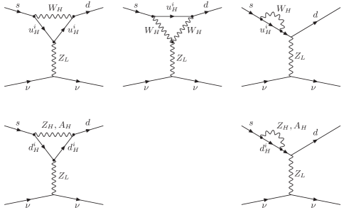
Figure 1: $Z_{L}$-penguin diagrams contributing in the T-odd sector.

There are two additional features with respect to the SM calculation and the box diagram calculation presented in [33] and below:

• The diagrams in Fig. 1 appear first to be ${\cal O}{(1)}$, that is they are not suppressed by $v^{2}/f^{2}$.

• The couplings of mirror fermions to $Z_{L}$ are vectorial ($\gamma^{\mu}$) in contrast to the SM couplings that have both $\gamma^{\mu}$ and $\gamma^{\mu}\gamma_{5}$ components.

Clearly the ${\cal O}(1)$ contributions have to vanish as otherwise it would not be possible to decouple the mirror fermions in the limit $f\to\infty$. This is assured by the vectorial coupling of $Z_{L}$ to the mirror fermions. The missing of diagrams with triple gauge boson vertices in the neutral gauge boson case is compensated by the difference between $\bar{d}^{i}_{H}Z_{L}^{\mu}d^{i}_{H}$ and $\bar{u}^{i}_{H}Z_{L}^{\mu}u^{i}_{H}$ couplings, so that the charged ($W_{H}^{\pm}$) and neutral ($Z_{H},\,A_{H}$) gauge boson contributions of ${\cal O}(1)$ to the $Z_{L}$-penguin vanish independently of each other in the unitary gauge.

As the inclusion of $v^{2}/f^{2}$ corrections to the neutral gauge boson interactions leads only to an overall factor multiplying the $Z_{H}$ and $A_{H}$ contributions, which vanish independently of each other, we find that there is no contribution from mirror fermions to $Z_{L}$-penguin diagrams in the unitary gauge. The inclusion of $v^{2}/f^{2}$ corrections to the relations between the masses of $u^{i}_{H}$ and $d^{i}_{H}$ and to the gauge boson masses does not change this result.

5.3 Box Diagrams in the Unitary Gauge

In order to simplify the formulae, we will present the results for the box diagrams shown in Fig. 2 in the limit of degenerate mirror leptons. As the box contributions vanish in the limit of degenerate mirror quarks, the inclusion of mass splittings in the lepton spectrum is a higher order effect. We have numerically verified that it can be neglected for the range of mirror fermion masses considered in the analysis.

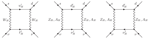
Figure 2: Box diagrams in the unitary gauge.

Let us begin with the neutral gauge boson contributions. Similarly to $\Delta F=2$ transitions considered in [32, 33], only the $g^{\mu\nu}$ part of the gauge boson propagators is relevant. The contributions involving $k^{\mu}k^{\nu}/M_{W_{H}}^{2}$ cancel each other between the two last sets of box diagrams in Fig. 2. Consequently the neutral gauge boson box contributions to $\bar{X}_{i}^{\text{odd}}$ and $\bar{Y}_{i}^{\text{odd}}$ are gauge independent. This means that the neutral gauge boson contributions to $Z_{L}$-penguins must vanish in an arbitrary gauge which is confirmed through an explicit calculation, as discussed below.

The result for the box contributions involving $W_{H}^{\pm}$ turns out to be divergent. As box contributions in a renormalizable gauge, like the ’t Hooft-Feynman gauge, are finite by power counting, the box diagram contributions involving $W_{H}^{\pm}$ must then be gauge dependent. Before giving the result for the unitary gauge calculation, including also neutral gauge boson contributions, let us repeat the calculation in the ’t Hooft-Feynman gauge.

5.4 Calculation in the ’t Hooft-Feynman Gauge

In the ’t Hooft-Feynman gauge also the diagrams with Goldstone bosons have to be included. Let us first compute the $Z_{L}$-penguin diagrams. The $\mathcal{O}\left(1\right)$ contributions vanish as expected and we have to consider $\mathcal{O}\left(v^{2}/f^{2}\right)$ corrections. Here, as in the unitary gauge, there are no contributions from diagrams involving only gauge bosons. On the other hand diagrams with Goldstone bosons contribute at $\mathcal{O}\left(v^{2}/f^{2}\right)$. To this end we had to generalize the Feynman rules of [32] to include $\mathcal{O}\left(v^{2}/f^{2}\right)$ corrections to vertices involving Goldstone bosons. It turns out that $\mathcal{O}\left(v^{2}/f^{2}\right)$ corrections to quark–mirror quark–Goldstone boson vertices cancel in the calculation, which implies that the neutral gauge boson contributions to the $Z_{L}$-penguin, not having triple gauge boson vertices and corresponding vertices with Goldstone bosons, vanish also in the ’t Hooft-Feynman gauge. This was to be expected as the box contributions from neutral gauge bosons are gauge independent.

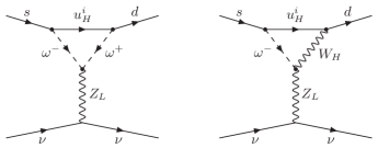
Figure 3: $\mathcal{O}\left(v^{2}/f^{2}\right)$ contributions to $Z_{L}$-penguin in the ’t Hooft-Feynman gauge.

Thus in the ’t Hooft-Feynman gauge only two diagrams at $\mathcal{O}\left(v^{2}/f^{2}\right)$, shown in Fig. 3, contribute to the $Z_{L}$-penguin vertex. Using the Feynman rules of Appendix B we find that the first diagram in Fig. 3 is divergent with the divergence precisely equal to the one found in box diagrams with $W_{H}^{\pm}$ exchanges calculated in the unitary gauge.

Including next the finite contributions from the diagrams in Fig. 3 and the finite contributions from box diagrams with $W_{H}^{\pm}$ and Goldstone boson exchanges in the ’t Hooft-Feynman gauge, we confirm the final results for $\bar{X}_{i}^{\text{odd}}$ and $\bar{Y}_{i}^{\text{odd}}$ obtained in the unitary gauge.

5.5 Final Results for the T-odd sector

As described above, we have performed the calculation of the functions $\bar{X}_{i}^{\text{odd}}$ and $\bar{Y}_{i}^{\text{odd}}$ in the unitary gauge and in the ’t Hooft-Feynman gauge obtaining the same results. In particular, we found that the left-over divergence obtained in the unitary gauge was not an artifact of a non-renormalizable gauge but a physical gauge independent result. A similar divergence has been found in the $Z_{L}$-penguin calculation in the LH model without T-parity [28]. We will recall the interpretation of this divergent contribution given in [28] in the next section.

The final results for $\bar{X}_{i}^{\text{odd}}$ and $\bar{Y}_{i}^{\text{odd}}$ in the LHT model are then given as follows:

$$\bar{X}_{i}^{\text{odd}} = \left[\xi_{2}^{(i)}\big{(}J^{\nu\bar{\nu}}(z_{2},y)-J^{\nu\bar{\nu}}(z_{1},y)\big{)}+\xi_{3}^{(i)}\big{(}J^{\nu\bar{\nu}}(z_{3},y)-J^{\nu\bar{\nu}}(z_{1},y)\big{)}\right],$$ (5.1)

$$\bar{Y}_{i}^{\text{odd}} = \left[\xi_{2}^{(i)}\big{(}J^{\mu\bar{\mu}}(z_{2},y)-J^{\mu\bar{\mu}}(z_{1},y)\big{)}+\xi_{3}^{(i)}\big{(}J^{\mu\bar{\mu}}(z_{3},y)-J^{\mu\bar{\mu}}(z_{1},y)\big{)}\right],$$ (5.2)

where

$$J^{\nu\bar{\nu}}\left(z_{i},y\right) = \frac{1}{64}\frac{v^{2}}{f^{2}}\bigg{[}z_{i}S_{\text{odd}}+F^{\nu\bar{\nu}}(z_{i},y;W_{H})$$ (5.3)

$$\qquad+4\Big{(}G(z_{i},y;Z_{H})+G_{1}(z^{\prime}_{i},y^{\prime};A_{H})+G_{2}(z_{i},y;\eta)\Big{)}\bigg{]},$$

$$J^{\mu\bar{\mu}}\left(z_{i},y\right) = \frac{1}{64}\frac{v^{2}}{f^{2}}\bigg{[}{z_{i}}S_{\text{odd}}+F^{\mu\bar{\mu}}(z_{i},y;W_{H})$$ (5.4)

$$\qquad-4\Big{(}G(z_{i},y;Z_{H})+G_{1}(z^{\prime}_{i},y^{\prime};A_{H})-G_{2}(z_{i},y;\eta)\Big{)}\bigg{]},$$

$$S_{\text{odd}} = \frac{1}{\varepsilon}+\log\frac{\mu^{2}}{M_{W_{H}}^{2}}\,,$$ (5.5)

with the functions $F^{\nu\bar{\nu}}$, $F^{\mu\bar{\mu}}$, $G$, $G_{1}$ and $G_{2}$ given in Appendix C and the various variables defined as follows

$$z_{i}=\frac{m_{Hi}^{2}}{M_{W_{H}}^{2}}=\frac{m_{Hi}^{2}}{M_{Z_{H}}^{2}}\,,\qquad z_{i}^{\prime}=az_{i}\quad\text{with }\;a=\frac{5}{\tan^{2}\theta_{W}}\,,$$ (5.6)

$$y=\frac{m_{H\ell}^{2}}{M_{W_{H}}^{2}}=\frac{m_{H\ell}^{2}}{M_{Z_{H}}^{2}}\,,\qquad y^{\prime}=ya\,,\quad\eta=\frac{1}{a}\,.$$ (5.7)

In the unitary gauge the results in (5.1)-(5.4) follow from box diagrams only, since the $Z_{L}$-penguin diagrams do not contribute in this gauge, as discussed in Section 5.2. The notation in (5.3) and (5.4) indicates which diagrams contribute to a given function, with $G_{2}$ resulting from diagrams with both $Z_{H}$ and $A_{H}$ exchanges. In the ’t Hooft-Feynman gauge the contribution of the $Z_{L}$-penguin diagram is found to be

$$\Delta J^{\nu\bar{\nu}}=\Delta J^{\mu\bar{\mu}}\equiv\overline{\Delta J}\frac{1}{64}\frac{v^{2}}{f^{2}}\,,$$ (5.8)

$$\overline{\Delta J}={z_{i}}{S_{\text{odd}}}-8z_{i}R_{2}(z_{i})+\frac{3}{2}z_{i}+2z_{i}F_{2}(z_{i})\,,$$ (5.9)

where the functions $R_{2}$ and $F_{2}$ are given in Appendix C.

The box diagram contribution involving $W_{H}^{\pm}$ in the ’t Hooft-Feynman gauge can simply be obtained from (5.1)-(5.4) and (5.8) using the gauge independence of $\bar{X}_{i}^{\text{odd}}$ and $\bar{Y}_{i}^{\text{odd}}$.

The formulae (5.1)-(5.4) are the main results of our paper.

6 The Issue of left-over Singularities

It may seem surprising that FCNC amplitudes considered in the previous section contain residual ultraviolet divergences reflected by the non-cancellation of the $1/\varepsilon$ poles at $\mathcal{O}\left(v^{2}/f^{2}\right)$ in our unitary gauge calculation. Indeed due to the GIM mechanism the FCNC processes considered here vanish at tree level both in the SM and in the LHT model in question. Therefore within the particle content of the low energy representation of the LHT model there seems to be no freedom to cancel the left-over divergences as the necessary tree level counter terms are absent.

At first sight one could worry that the remaining divergence is an artifact of the unitary gauge calculation. However, an additional calculation in the ’t Hooft-Feynman gauge convinced us that the found divergence is gauge independent. A similar result has been found in the context of the LH model without T-parity in [28] and understood as the sensitivity of the decay amplitudes to the UV completion of the LH model. The same interpretation can be made here. After all, the LHT model is a non-linear sigma model, which is a non-renormalizable description of the low energy behavior of a symmetric theory below the scale where the symmetry is dynamically broken.

We have found explicitly that in the ’t Hooft-Feynman gauge the singularity followed entirely from the interactions of the Goldstone bosons of the dynamically broken global symmetry with the fermions. As the Goldstone bosons in question are the only reminiscences of the spontaneous symmetry breakdown present in the low energy theory, the estimate of the size of the divergences through their interactions with fermions in Fig. 3 should in principle be adequate. However, as emphasized in [28], the light fermions may have a more complex relation to the fundamental fermions of the ultraviolet completion of the theory. We refer the reader to [28], where a discussion of this issue and a comparison with QCD can be found.

In what follows we will as in [28] remove $1/\varepsilon$ terms from (5.5) and set $\mu=\Lambda$ to obtain

$$J^{\nu\bar{\nu}}_{\text{div}}=J^{\mu\bar{\mu}}_{\text{div}}=z_{i}\frac{1}{64}\frac{v^{2}}{f^{2}}\log\frac{\Lambda^{2}}{M_{W_{H}}^{2}}\,,$$ (6.1)

as a minimal estimate of the UV sensitivity of the model. Setting

$$\Lambda=4\pi f\,,\qquad\qquad v=246\,{\rm GeV}\,,$$ (6.2)

we find that for $f=1000\,{\rm GeV}$, implying $M_{W_{H}}=652\,{\rm GeV}$,

$$J^{\nu\bar{\nu}}_{\text{div}}=J^{\mu\bar{\mu}}_{\text{div}}=z_{i}\cdot 0.006\,.$$ (6.3)

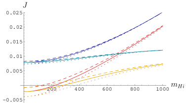
Figure 4: $J^{\nu\bar{\nu}}$ (lower) and $J^{\mu\bar{\mu}}$ (upper) as functions of $m_{Hi}$ for values of $m_{H\ell}=$400 GeV(dotted), 500 GeV (solid) and 600 GeV (dashed) with (dark) and without (light) $J^{\nu\bar{\nu}}_{\text{div}}=J^{\mu\bar{\mu}}_{\text{div}}$ included.

In Fig. 4 we plot $J^{\nu\bar{\nu}}$ and $J^{\mu\bar{\mu}}$ as functions of $m_{Hi}$ for three values of $m_{H\ell}$ with and without $J^{\nu\bar{\nu}}_{\text{div}}$ and $J^{\mu\bar{\mu}}_{\text{div}}$ included. We observe that the divergences constitute a sizable fraction of the total result. The coefficient of $z_{i}$ in the divergent terms $J^{\nu\bar{\nu}}_{\text{div}}$ and $J^{\mu\bar{\mu}}_{\text{div}}$ is of the same order of magnitude of the analogous linear coefficient in the convergent contributions, but roughly four times larger. Moreover, the linear contribution in the range of mirror fermion masses considered is the dominant one, thus explaining the important impact of the divergences. At first sight this could imply the loss of the predictive power of the theory as our estimate of the divergent contribution is clearly an approximation. On the other hand the divergence found has a universal character and we can simply write

$$J^{\nu\bar{\nu}}_{\text{div}}=J^{\mu\bar{\mu}}_{\text{div}}=\delta_{\text{div}}\,z_{i}$$ (6.4)

and treat $\delta_{\text{div}}$ as a free parameter. Assuming that $\delta_{\text{div}}$ encloses all effects coming from the UV completion, which is true if light fermions do not have a more complex relation to the fundamental fermions of the UV completion that could spoil its flavour independence, one can in principle fit $\delta_{\text{div}}$ to the data and trade it for one observable. At present this is not feasible, but could become realistic when more data for FCNC processes will be available.

On the other hand, implementing T-parity removes all divergences from the T-even sector. This is easy to understand. The only new T-even particle is $T_{+}$ which can be thought of as an arbitrary singlet field mixing with the SM top quark, independently of the non-linear sigma model. Of the “pion” matrix $\Pi$, only the SM Higgs doublet is present in the T-even sector, and all modifications in its couplings appear due to the mixing of $T_{+}$ with $t$. Thus the T-even sector of the LHT model is effectively decoupled from the breaking $SU(5)\to SO(5)$ of the non-linear sigma model, which has been the basic reason for the appearance of the singularity described above and in [28].

7 $B\to X_{s}\ell^{+}\ell^{-}$

7.1 Preliminaries

The branching ratio for the rare decay $B\to X_{s}\ell^{+}\ell^{-}$ depends in the SM on the functions $Y_{\rm SM}$, $Z_{\rm SM}$ and $D^{\prime}_{\rm SM}$ with the latter relevant also for the $B\to X_{s}\gamma$ decay. The formulae for the branching ratio are very complicated and will not be presented here. They can be found in [57], where also the formulae for the forward-backward asymmetries are given. In the LHT model the function $Y_{\rm SM}$ is generalized to $Y_{s}$ calculated in the previous section, whereas $D^{\prime}_{\rm LHT}$ has been calculated in [33] and is given for completeness in Appendix C.

What remains to be calculated is the function $Z_{s}$ that we defined in (3.5). The SM contribution can be written as

$$Z_{\rm SM}=C_{0}+\frac{1}{4}D_{0}$$ (7.1)

with $C_{0}$ and $D_{0}$ given in the ’t Hooft-Feynman gauge in Appendix C. $Z_{\rm SM}$ is gauge independent. We will also need the QCD-penguin function $E_{0}$ that can be found in Appendix C as well.

7.2 T-even Sector

In the case of the T-even sector it is useful to work in the unitary gauge. The function $C_{\rm even}$ can be extracted from [28] by imposing T-parity with the result

$$C^{\rm even}_{\text{unitary}} = \frac{x_{L}^{2}}{8}\frac{v^{2}}{f^{2}}S_{\text{even}}\left(\frac{x_{t}-x_{T}}{2}-d_{2}x_{T}\frac{v^{2}}{f^{2}}\right)$$ (7.2)

$$-\frac{x_{L}^{2}}{16}\frac{v^{2}}{f^{2}}\bigg{(}\frac{-6-5x_{t}+5x_{t}^{2}-3x_{T}+3x_{t}x_{T}}{2(x_{t}-1)}$$

$$\qquad+\frac{8x_{t}-10x_{t}^{2}+5x_{t}^{3}}{(x_{t}-1)^{2}}\log x_{t}-(4x_{t}+x_{T})\log x_{T}\bigg{)}$$

$$+\frac{x_{L}^{2}}{8}\frac{v^{4}}{f^{4}}x_{T}\left(-\frac{3}{2}d_{2}+x_{L}^{2}+d_{2}\log x_{T}\right)\,,$$

where

$$S_{\text{even}}=\frac{1}{\varepsilon}+\log\frac{\mu^{2}}{M_{W_{L}}^{2}}\,,$$ (7.3)

and $d_{2}$ has been defined in (2.34).

The function $D_{\rm even}$ in the LHT model can be obtained with the help of $D_{\rm SM}$ in the unitary gauge. To our knowledge the latter function has never been given in this gauge in the literature. It can be found with the help of [28] as follows.

From the gauge independence of $Z_{\rm SM}$ we know that

$$C_{\text{SM}}=C_{0}+\frac{1}{2}\bar{\varrho}_{\text{SM}}\,,\qquad D_{\text{SM}}=D_{0}-2\bar{\varrho}_{\text{SM}}\,,$$ (7.4)

where $\bar{\varrho}_{\text{SM}}$ is gauge dependent and vanishes in the ’t Hooft-Feynman gauge. It has been calculated in the unitary gauge in [28] with the result

$$\bar{\varrho}_{\text{SM}}=-\frac{1}{8}{x_{t}}{S_{\text{even}}}-\frac{-3x_{t}^{2}+17x_{t}}{16(1-x_{t})}-\frac{8x_{t}^{2}-x_{t}^{3}}{8(x_{t}-1)^{2}}\log x_{t}\,.$$ (7.5)

Consequently, using $D_{0}$ in Appendix C, we find

$$D^{\text{SM}}_{\rm unitary}(x_{t}) = \frac{x_{t}}{4}S_{\text{even}}+\frac{-153x_{t}+383x_{t}^{2}-245x_{t}^{3}+27x_{t}^{4}}{72(x_{t}-1)^{3}}$$ (7.6)

$$-\frac{16-64x_{t}+36x_{t}^{2}+93x_{t}^{3}-84x_{t}^{4}+9x_{t}^{5}}{36(x_{t}-1)^{4}}\log x_{t}\,.$$

Proceeding then as in the case of $B\to X_{s}\gamma$ in [28] but including also $v^{4}/f^{4}$ corrections to the diagrams with internal $T_{+}$ exchanges we find

$$D^{\rm even}_{\text{unitary}}=\frac{v^{2}}{f^{2}}x_{L}^{2}\left[\left(1+2d_{2}\frac{v^{2}}{f^{2}}\right)D^{\text{SM}}_{\rm unitary}(x_{T})-D^{\text{SM}}_{\rm unitary}(x_{t})\right]\,,$$ (7.7)

and, dropping $\mathcal{O}(v^{4}/f^{4})$ terms,

$$D^{\rm even}_{\text{unitary}} = \frac{v^{2}}{f^{2}}x_{L}^{2}\left[\frac{x_{T}}{4}\left(1+2d_{2}\frac{v^{2}}{f^{2}}\right)S_{\rm even}-D^{\text{SM}}_{\rm unitary}(x_{t})\right]$$ (7.8)

$$+\frac{v^{2}}{f^{2}}x_{L}^{2}\left[-\frac{41-24\log x_{T}}{18}+\frac{x_{T}}{8}\left(1+2d_{2}\frac{v^{2}}{f^{2}}\right)(3-2\log x_{T})\right]\,,$$

and subsequently

$$\bar{Z}_{\rm even}=C^{\rm even}_{\rm unitary}+\frac{1}{4}D^{\rm even}_{\rm unitary}$$ (7.9)

which is gauge independent. The divergence $S_{\text{even}}$ cancels in (7.9) so that $\bar{Z}_{\text{even}}$ is finite, in agreement with our statement in Section 6.

7.3 T-odd Sector

In the T-odd sector it is useful to work in the ’t Hooft-Feynman gauge. Let us denote

$$Z_{\rm odd}(z_{i})=C_{\rm odd}(z_{i})+\frac{1}{4}D_{\rm odd}(z_{i})\,,$$ (7.10)

then, from (5.8) and (5.9), we find in the ’t Hooft-Feynman gauge

$$C_{\rm odd}(z_{i})=\Delta J^{\mu\bar{\mu}}=\frac{1}{64}\frac{v^{2}}{f^{2}}\left[{z_{i}}{S_{\text{odd}}}-8z_{i}R_{2}(z_{i})+\frac{3}{2}z_{i}+2z_{i}F_{2}(z_{i})\right]$$ (7.11)

with $S_{\text{odd}}$ defined in (5.5) and the functions $R_{2}$ and $F_{2}$ given in Appendix C.

$D_{\rm odd}(z_{i})$ is then found in analogy to our calculation of the $B\to X_{s}\gamma$ decay in [33]. We obtain

$$D_{\rm odd}(z_{i})=\frac{1}{4}\frac{v^{2}}{f^{2}}\left[D_{0}(z_{i})-\frac{1}{6}E_{0}(z_{i})-\frac{1}{30}E_{0}(z^{\prime}_{i})\right]$$ (7.12)

with $D_{0}$ and $E_{0}$ given in Appendix C. Finally we have

$$\bar{Z}_{s}^{\rm odd}=\bigg{[}\xi^{(s)}_{2}\big{(}Z_{\rm odd}(z_{2})-Z_{\rm odd}(z_{1})\big{)}+\xi^{(s)}_{3}\big{(}Z_{\rm odd}(z_{3})-Z_{\rm odd}(z_{1})\big{)}\bigg{]}\,.$$ (7.13)

As $D_{\rm odd}(z_{i})$ is finite, the divergence in $C_{\rm odd}(z_{i})$ remains in $Z_{\text{odd}}$. Its estimate can be done as outlined in Section 6.

8 $K_{L}\to\pi^{0}\ell^{+}\ell^{-}$

The rare decays $K_{L}\to\pi^{0}e^{+}e^{-}$ and $K_{L}\to\pi^{0}\mu^{+}\mu^{-}$ are dominated by CP-violating contributions. In the SM the main contribution comes from the indirect (mixing-induced) CP violation and its interference with the direct CP-violating contribution [58, 59, 60, 61]. The direct CP-violating contribution to the branching ratio is in the ballpark of $4\cdot 10^{-12}$, while the CP conserving contribution is at most $3\cdot 10^{-12}$. Among the rare $K$ meson decays, the decays in question belong to the theoretically cleanest, but certainly cannot compete with the $K\to\pi\nu\bar{\nu}$ decays. Moreover, the dominant indirect CP-violating contributions are practically determined by the measured decays $K_{S}\to\pi^{0}\ell^{+}\ell^{-}$ and the parameter $\varepsilon_{K}$. Consequently they are not as sensitive as the $K_{L}\to\pi^{0}\nu\bar{\nu}$ decay to new physics contributions, present only in the subleading direct CP violation. However, as pointed out in [37], in the presence of large new CP-violating phases the direct CP-violating contribution can become the dominant contribution and the branching ratios for $K_{L}\to\pi^{0}\ell^{+}\ell^{-}$ can be enhanced by a factor of 2–3, with a stronger effect in the case of $K_{L}\to\pi^{0}\mu^{+}\mu^{-}$ [60, 61].

Adapting the formulae in [59, 60, 61, 62] with the help of [37] to the LHT model we find

$$Br(K_{L}\to\pi^{0}\ell^{+}\ell^{-})=\left(C_{\text{dir}}^{\ell}\pm C_{\text{int}}^{\ell}\left|a_{s}\right|+C_{\text{mix}}^{\ell}\left|a_{s}\right|^{2}+C_{\text{CPC}}^{\ell}\right)\cdot 10^{-12}\,,$$ (8.1)

where

$$C_{\text{dir}}^{e}=(4.62\pm 0.24)(\omega_{7V}^{2}+\omega_{7A}^{2})\,, C_{\text{dir}}^{\mu}=(1.09\pm 0.05)(\omega_{7V}^{2}+2.32\omega_{7A}^{2})\,,$$ (8.2)

$$C_{\text{int}}^{e}=(11.3\pm 0.3)\omega_{7V}\,, C_{\text{int}}^{\mu}=(2.63\pm 0.06)\omega_{7V}\,,$$ (8.3)

$$C_{\text{mix}}^{e}=14.5\pm 0.05\,, C_{\text{mix}}^{\mu}=3.36\pm 0.20\,,$$ (8.4)

$$C_{\text{CPC}}^{e}\simeq 0\,, C_{\text{CPC}}^{\mu}=5.2\pm 1.6\,,$$ (8.5)

$$\left|a_{s}\right|=1.2\pm 0.2$$ (8.6)

with

$$\omega_{7V} = \frac{1}{2\pi}\left[P_{0}+\frac{|Y_{K}|}{\sin^{2}\theta_{W}}\frac{\sin\beta^{K}_{Y}}{\sin(\beta-\beta_{s})}-4|Z_{K}|\frac{\sin\beta^{K}_{Z}}{\sin(\beta-\beta_{s})}\right]\left[\frac{{\rm Im}\,\lambda_{t}}{1.4\cdot 10^{-4}}\right]\,,$$ (8.7)

$$\omega_{7A} = -\frac{1}{2\pi}\frac{|Y_{K}|}{\sin^{2}\theta_{W}}\frac{\sin\beta^{K}_{Y}}{\sin(\beta-\beta_{s})}\left[\frac{{\rm Im}\,\lambda_{t}}{1.4\cdot 10^{-4}}\right]\,,$$ (8.8)

where $P_{0}=2.88\pm 0.06$ [63] includes NLO QCD corrections and

$$\beta^{K}_{Y}=\beta-\beta_{s}-\theta^{K}_{Y}\,,\qquad\beta^{K}_{Z}=\beta-\beta_{s}-\theta^{K}_{Z}$$ (8.9)

with $Z_{K}$ defined in (3.5) and obtained from $Z_{s}$ by changing $\xi^{(s)}_{i}$ to $\xi^{(K)}_{i}$.

The effect of the new physics contributions is mainly felt in $\omega_{7A}$, as the corresponding contributions in $\omega_{7V}$ cancel each other to a large extent.

The present experimental bounds

$$Br(K_{L}\to\pi^{0}e^{+}e^{-})<28\cdot 10^{-11}\quad\text{\cite[cite]{[\@@bibref{}{Alavi-Harati:2003}{}{}]}}\,,\qquad Br(K_{L}\to\pi^{0}\mu^{+}\mu^{-})<38\cdot 10^{-11}\quad\text{\cite[cite]{[\@@bibref{}{Alavi-Harati:2000}{}{}]}}$$ (8.10)

are still by one order of magnitude larger than the SM predictions [62]

$$Br(K_{L}\to\pi^{0}e^{+}e^{-})_{\text{SM}}=3.54^{+0.98}_{-0.85}\left(1.56^{+0.62}_{-0.49}\right)\cdot 10^{-11}\,,$$ (8.11)

$$Br(K_{L}\to\pi^{0}\mu^{+}\mu^{-})_{\text{SM}}=1.41^{+0.28}_{-0.26}\left(0.95^{+0.22}_{-0.21}\right)\cdot 10^{-11}$$ (8.12)

with the values in parentheses corresponding to the “$-$” sign in (8.1).

9 Benchmark Scenarios for New Parameters

9.1 Preliminaries

In what follows, we will consider as in [33] several scenarios for the structure of the $V_{Hd}$ matrix and the mass spectrum of mirror fermions with the hope to gain a global view about the possible signatures of mirror fermions in the processes considered and of $T_{+}$ present in the T-even contributions.

In the most interesting scenario considered in [33] (Scenario $4$ below), the mixing matrix $V_{Hd}$ differed significantly from $V_{\text{CKM}}$. It could have a large non-vanishing complex phase $\delta_{13}^{d}$, while the phases $\delta_{12}^{d}$ and $\delta_{23}^{d}$, with smaller phenomenological impact, were set to zero. In this scenario large CP-violating effects in $B_{s}$ decays have been found. In particular, the CP asymmetries $S_{\psi\phi}$ and $A^{s}_{\text{SL}}$ could be enhanced by an order of magnitude with respect to the SM expectations.

In the next section we will be primarily interested in calculating the observables considered in the previous sections in the scenarios defined in [33]. In particular, it will be interesting to see how the CMFV correlations between $K^{0}$, $B^{0}_{d}$ and $B_{s}^{0}$ systems [40, 67] are modified when new sources of flavour and CP violation are present. The parameterization of various decays in terms of the functions $X_{i}$, $Y_{i}$ and $Z_{i}$ that we defined in Section 3 is very useful for such tests.

The main purpose of our numerical analysis is to have a closer look at six scenarios, with the first five considered already in our previous study of particle-antiparticle mixing and $B\to X_{s}\gamma$. We will recall these five scenarios and introduce a sixth one which has particularly interesting effects in $K\to\pi\nu\bar{\nu}$ and $K_{L}\to\pi^{0}\ell^{+}\ell^{-}$ decays. In all these six scenarios we set the phases $\delta_{12}^{d}$ and $\delta_{23}^{d}$ to zero. The values of the observables that can only be produced by allowing these phases to vary freely, are covered by our general scan anyway. This simplification therefore does not restrict the generality of the analysis. We will see that Scenarios $4$ and $6$ turn out to be the most appealing, since they respectively provide large enhancements in the $B_{s}$ and $K$ systems. Spectacular effects in both $B$ and $K$ systems, however, are not simultaneously allowed in a single scenario. Therefore, we complete the numerical analysis with a general scan over mirror fermion masses and $V_{Hd}$ parameters, with also $\delta_{12}^{d}$ and $\delta_{23}^{d}$ free to differ from zero, finding some interesting points where significant enhancements in both $B$ and $K$ systems occur.

9.2 Different Scenarios

Here we just list the scenarios in question:

Scenario 1:

In this scenario the mirror fermions will be degenerate in mass

$$m_{H1}=m_{H2}=m_{H3}$$ (9.1)

and only the T-even sector will contribute. This is the MFV limit of the LHT model.

Scenario 2:

In this scenario the mirror fermions are not degenerate in mass and

$$V_{Hd}=V_{\text{CKM}}\,.$$ (9.2)

In this case there are no contributions of mirror fermions to $D^{0}-\bar{D}^{0}$ mixing and flavour violating $D$ meson decays, and

$$\xi_{2}^{(q)}=\lambda_{c}^{(q)}\,,\qquad\xi_{3}^{(q)}=\lambda_{t}^{(q)}\,,$$ (9.3)

with $q=d,s$ and no index $q$ in the $K$ system. As discussed in [33] and below this scenario differs from the MFV case.

Scenario 3:

In this scenario we will choose a linear spectrum for mirror quarks

$$m_{H1}=400\,{\rm GeV},\qquad m_{H2}=500\,{\rm GeV},\qquad m_{H3}=600\,{\rm GeV}\,,$$ (9.4)

set $m_{H\ell}=500\,{\rm GeV}$ and take an arbitrary matrix $V_{Hd}$ but with the phases $\delta_{12}^{d}$ and $\delta_{23}^{d}$ set to zero. We stress that similar results are obtained by changing the values above by $\pm 30\,{\rm GeV}$, with similar comments applying to (9.5) below. In the remaining scenarios we will modify the mirror quark spectrum but keep $m_{H\ell}=500\,{\rm GeV}$.

Scenario 4:

This was our favorite scenario in which large departures from the SM and MFV in $B_{s}$ decays could be obtained and some problems addressed in [33] could be solved, with small effects in the experimentally well measured quantities $\Delta M_{K}$ and $\varepsilon_{K}$. In this scenario

$$m_{H1}\approx m_{H2}=500\,{\rm GeV}\,,\qquad m_{H3}=1000\,{\rm GeV}\,,$$ (9.5)

$$\frac{1}{\sqrt{2}}\leq s_{12}^{d}\leq 0.99\,,\qquad 5\cdot 10^{-5}\leq s_{23}^{d}\leq 2\cdot 10^{-4}\,,\qquad 4\cdot 10^{-2}\leq s_{13}^{d}\leq 0.6\,,$$ (9.6)

$\delta_{12}^{d}$ and $\delta_{23}^{d}$ are set to zero, while the phase $\delta^{d}_{13}$ is arbitrary. The hierarchical structure of the CKM matrix

$$s_{13}\ll s_{23}\ll s_{12}\,,\qquad(\text{CKM})$$ (9.7)

is changed in this scenario to

$$s^{d}_{23}\ll s^{d}_{13}\leq s^{d}_{12}\,,\qquad(V_{Hd})$$ (9.8)

so that $V_{Hd}$ looks as follows:

$$V_{Hd}=\begin{pmatrix}c^{d}_{12}&s^{d}_{12}&s^{d}_{13}e^{-i\delta^{d}_{13}}\\ -s^{d}_{12}&c^{d}_{12}&s^{d}_{23}\\ -c^{d}_{12}s^{d}_{13}e^{i\delta^{d}_{13}}&-s^{d}_{12}s^{d}_{13}e^{i\delta^{d}_{13}}&1\end{pmatrix}.$$ (9.9)

We would like to stress that with the degeneracy $m_{H1}\approx m_{H2}$ the T-odd contributions in $\varepsilon_{K}$ proportional to ${\rm Im}(\xi_{2})$ and ${\rm Re}(\xi_{2})$ vanish, and only the T-odd term proportional to ${\rm Im}(\xi_{3}){\rm Re}(\xi_{3})$ contributes. Being ${\rm Im}(\xi_{3})=s^{d}_{13}c^{d}_{23}s^{d}_{23}\sin\delta^{d}_{13}$, the hierarchy chosen in this scenario for $V_{Hd}$, with $s^{d}_{23}\ll 1$, has the advantage of suppressing mirror fermion effects in $\varepsilon_{K}$, allowing at the same time large CP-violating effects in the $B^{0}_{s}-\bar{B}^{0}_{s}$ system [33]. Furthermore $\Delta M_{s}$ can be smaller than its SM value in this scenario, and interesting effects in the $B^{0}_{d}-\bar{B}^{0}_{d}$ system are also found.

It will be interesting to see whether in this scenario large departures from the SM expectations for rare decays can be obtained.

Scenario 5:

In all the previous scenarios we will choose the first solution for the angle $\gamma$ from tree level decays as given in (10.1) below so that only small departures from the SM in the $B^{0}_{d}-\bar{B}^{0}_{d}$ system will be consistent with the data. In the present scenario one assumes the second solution for $\gamma$ in (10.1) in contradiction with the SM and MFV. We have shown in [33] that the presence of new flavour violating interactions could still bring the theory to roughly agree with the available data, in particular with the asymmetry $S_{\psi K_{S}}$. In spite of that, the combined measurements on $A^{d}_{\text{SL}}$ and $\cos(2\beta+2\varphi_{B_{d}})$ and the indirect experimental estimate of $A^{s}_{\text{SL}}$ make this scenario very unlikely [33, 68], such that we will not consider it any further.

Scenario 6:

In studying this scenario we aim to enhance mirror fermion contributions to rare $K$ decays, keeping negligible effects in the experimentally well measured quantities $\Delta M_{K}$ and $\varepsilon_{K}$. To this purpose we choose the mirror fermion masses as in Scenario 4 (see (9.5)) since the near degeneracy between $m_{H1}$ and $m_{H2}$ helps to suppress mirror fermion effects in $\Delta M_{K}$.

Concerning $\varepsilon_{K}$, we recall that with the degeneracy $m_{H1}\approx m_{H2}$ the T-odd contributions proportional to ${\rm Im}(\xi_{2})$ and ${\rm Re}(\xi_{2})$ vanish, and only the T-odd term proportional to ${\rm Im}(\xi_{3}){\rm Re}(\xi_{3})$ contributes. In Scenario $4$ the hierarchical structure of $V_{Hd}$ is chosen as to satisfy ${\rm Im}(\xi_{3})\simeq 0$. Here in Scenario $6$, instead, we suppress mirror fermion effects in $\varepsilon_{K}$ due to the second and third generations, by requiring ${\rm Re}(\xi_{3})=0$. Setting also in this scenario the phases $\delta_{12}^{d}$ and $\delta_{23}^{d}$ to zero, the explicit expression of the real part reads

$${\rm Re}(\xi_{3})=-c_{12}^{d}s_{12}^{d}\left({s_{23}^{d}}^{2}-{c_{23}^{d}}^{2}{s_{13}^{d}}^{2}\right)+(\cos\delta^{d}_{13})\,c_{23}^{d}s_{23}^{d}s_{13}^{d}\left({c_{12}^{d}}^{2}-{s_{12}^{d}}^{2}\right)\,,$$ (9.10)

which vanishes for $\theta_{12}^{d}$, $\theta_{23}^{d}$ and $\theta_{13}^{d}$ (chosen in the first quadrant) satisfying

$$c_{12}^{d}=s_{12}^{d}=\frac{1}{\sqrt{2}}\,,$$ (9.11)

$$s_{23}^{d}=\frac{s_{13}^{d}}{\sqrt{1+{s_{13}^{d}}^{2}}}\,.$$ (9.12)

We note that while the value of $\theta_{12}^{d}$ is fixed to $45^{\circ}$ by (9.11), $\theta_{23}^{d}$ and $\theta_{13}^{d}$ have no specified value nor order of magnitude, but (9.12) implies that only one of them is a free parameter. The matrix $V_{Hd}$ can then be expressed in terms of the two free parameters $\theta_{13}^{d}$ and $\delta^{d}_{13}$ as

$$V_{Hd}=\left(\begin{array}[]{ccc}\frac{c_{13}^{d}}{\sqrt{2}}&\frac{c_{13}^{d}}{\sqrt{2}}&s_{13}^{d}e^{-i\delta^{d}_{13}}\\ -\frac{1}{\sqrt{2}\sqrt{1+{s_{13}^{d}}^{2}}}(1+{s_{13}^{d}}^{2}e^{i\delta^{d}_{13}})&\frac{1}{\sqrt{2}\sqrt{1+{s_{13}^{d}}^{2}}}(1-{s_{13}^{d}}^{2}e^{i\delta^{d}_{13}})&\frac{s_{13}^{d}c_{13}^{d}}{\sqrt{1+{s_{13}^{d}}^{2}}}\\ \frac{s_{13}^{d}}{\sqrt{2}\sqrt{1+{s_{13}^{d}}^{2}}}(1-e^{i\delta^{d}_{13}})&-\frac{s_{13}^{d}}{\sqrt{2}\sqrt{1+{s_{13}^{d}}^{2}}}(1+e^{i\delta^{d}_{13}})&\frac{c_{13}^{d}}{\sqrt{1+{s_{13}^{d}}^{2}}}\end{array}\right).$$ (9.13)

Its structure becomes much simpler if the angle $\theta_{13}^{d}$ is sufficiently small, i. e., $s_{13}^{d}\leq 0.1$, and reads

$$V_{Hd}\approx\begin{pmatrix}\frac{1}{\sqrt{2}}&\frac{1}{\sqrt{2}}&s_{13}^{d}e^{-i\delta^{d}_{13}}\\ -\frac{1}{\sqrt{2}}&\frac{1}{\sqrt{2}}&s_{13}^{d}\\ \frac{s_{13}^{d}}{\sqrt{2}}(1-e^{i\delta^{d}_{13}})&-\frac{s_{13}^{d}}{\sqrt{2}}(1+e^{i\delta^{d}_{13}})&1\end{pmatrix}.$$ (9.14)

As we will see in Section 10 the very different structure of $V_{Hd}$ when compared with $V_{\rm CKM}$ implies enhancements in rare $K$ decays, without introducing problematic effects in $\Delta M_{K}$ and $\varepsilon_{K}$. Moreover, as $V_{Hd}$ in (9.14) has a different structure also from the (9.9) one of Scenario 4, the new physics effects in the $B^{0}_{d}-\bar{B}^{0}_{d}$ and mainly in the $B^{0}_{s}-\bar{B}^{0}_{s}$ system, turn out to be small although visible.

General Scan:

As shown in Section 10, Scenarios $4$ and $6$ turn out to be the most interesting ones with, respectively, large new physics effects in the $B_{s}$ and $K$ systems. Such visible enhancements follow from the structure of $V_{Hd}$, primarily required to satisfy the $\varepsilon_{K}$ and $\Delta M_{K}$ constraints, through ${\rm Im}(\xi_{3})\approx 0$ in Scenario $4$ and through ${\rm Re}(\xi_{3})=0$ in Scenario $6$. A further consequence of the $V_{Hd}$ structure is that in Scenario $4$ spectacular effects can be obtained in the $B_{s}$ system but not in the $K$ system and vice versa in Scenario $6$. An even more interesting picture would be the simultaneous manifestation of large enhancements in both $B$ and $K$ observables. In order not to miss such a possibility, in addition to the scenarios described above, we have performed a general scan over mirror fermion masses and $V_{Hd}$ parameters. To have a global view of the most general LHT effects, we have allowed here the phases $\delta_{12}^{d}$ and $\delta_{23}^{d}$ to differ from zero. Qualitatively their effect is not significant, although they can help in achieving very large effects in certain observables. We find that there exist some sets of masses and $V_{Hd}$ parameters where the new physics effects turn out to be spectacular in both $B$ and $K$ systems. We note that they do not really constitute a scenario, they rather appear in the plots shown in the next section as isolated (blue) points. In contrast to previous scenarios, in fact, the blue points corresponding to large new physics effects are quite sensitive to the particular configuration of mirror fermion masses and $V_{Hd}$ parameters.

10 Numerical Analysis

10.1 Preliminaries

In our numerical analysis we will set $|V_{us}|$, $|V_{cb}|$ and $|V_{ub}|$ to their central values measured in tree level decays [69, 70] and collected in Table 1.

$|V_{ub}|=0.00429(29)$	$G_{F}=1.16637(1)\cdot 10^{-5}\,{\rm GeV}^{-2}$
$|V_{cb}|=0.0416(9)$ [69]	$M_{\rm W}=80.425(38)\,{\rm GeV}$
$\lambda=|V_{us}|=0.225(1)$ [70]	$\alpha=1/127.9$
$|V_{ts}|=0.0409(9)$ [68]	$\sin^{2}\theta_{W}=0.23120(15)$
$A=0.822(16)$	$m_{K^{0}}=497.65(2)\,{\rm MeV}$
$R_{b}=0.447(31)$	$m_{B_{d}}=5.2794(5)\,{\rm GeV}$
$\beta=26.3(21)^{\circ}$	$m_{B_{s}}=5.370(2)\,{\rm GeV}$
$\beta_{s}=-1.28(7)^{\circ}$	$F_{K}=160(1)\,{\rm MeV}$ [71]
$\overline{m}_{\rm c}=1.30(5)\,{\rm GeV}$	$F_{B_{d}}=189(27)\,{\rm MeV}$
$\overline{m}_{\rm t}=163.8(32)\,{\rm GeV}$	$F_{B_{s}}=230(30)\,{\rm MeV}$   [72]

Table 1: Values of the experimental and theoretical quantities used as input parameters.

As the fourth parameter we will choose the angle $\gamma$ of the standard unitarity triangle that to an excellent approximation equals the phase $\delta_{\text{CKM}}$ in the CKM matrix. The angle $\gamma$ has been extracted from $B\to D^{(*)}K$ decays without the influence of new physics with the result [68]

$$\gamma=(71\pm 16)^{\circ}\,,\qquad\gamma=-(109\pm 16)^{\circ}\,.$$ (10.1)

Only the first solution agrees with the SM analysis of the unitarity triangle, while the consistency of the second solution with data has been investigated within Scenario 5 in our previous LHT analysis [33]. It turns out that the combined measurements on $A^{d}_{\text{SL}}$ and $\cos(2\beta+2\varphi_{B_{d}})$ and the indirect experimental estimate of $A^{s}_{\text{SL}}$ make this scenario very unlikely [33, 68].

We will consider here only the first solution, whose uncertainty is sufficiently large to allow for significant contributions from new physics. The value of $\beta$ in Table 1 is obtained from $R_{b}$ and the first solution of $\gamma$, i.e. from tree level decays only and is not affected by an eventual new physics phase. Its difference from the value of $\beta$ obtained from the $S_{\psi K_{S}}$ asymmetry, $\beta(\psi K_{S})=21.2\pm 1.0$, constitutes the “$\sin 2\beta$ problem” which can be solved only in Scenarios $3-6$ [33].

For the non-perturbative parameters entering the analysis of particle-antiparticle mixing we choose and collect in Table 1 their lattice averages given in [72], which combine unquenched results obtained with different lattice actions. Other parameters relevant for particle-antiparticle mixing can be found in [33].

In order to simplify our numerical analysis we will, as in [33], set all non-perturbative parameters to their central values and instead we will allow $\Delta M_{K}$, $\varepsilon_{K}$, $\Delta M_{d}$, $\Delta M_{s}$ and $S_{\psi K_{S}}$ to differ from their experimental values by $\pm 50\%$, $\pm 40\%$, $\pm 40\%$, $\pm 40\%$ and $\pm 8\%$, respectively. In the case of $\Delta M_{s}/\Delta M_{d}$ we will choose $\pm 20\%$ as the error on the relevant parameter, $\xi$, is smaller than in the case of $\Delta M_{d}$ and $\Delta M_{s}$ separately. The relevant expressions are given in [33]. These uncertainties could appear rather conservative, but we do not want to miss any interesting effect by choosing too optimistic non-perturbative uncertainties. The constraints from $B\to X_{s}\gamma$ and $B\to X_{s}\ell^{+}\ell^{-}$ are also taken into account. They turn out to be easily satisfied, within the present uncertainties, and therefore to have only a minor impact.

In Scenarios $3-6$, the parameters $f$ and $x_{L}$ will be fixed to $f=1000\,{\rm GeV}$ and $x_{L}=0.5$ in accordance with electroweak precision tests [30]. Varying the breaking scale $f$ would obviously modify our results. The effect, however, turns out to be much smaller than one would naively expect from the $v^{2}/f^{2}-$“scaling”. In other words, lower values of $f$ do not allow arbitrarily large NP contributions, since the constraints imposed from the available data become more stringent in this case.

10.2 The MFV Scenario 1

Let us consider first the case of totally degenerate mirror fermions. In this case the odd contributions vanish due to the GIM mechanism [47], the only new particle contributing is $T_{+}$ and the LHT model in this limit belongs to the class of MFV models. As only the T-even sector contributes, the new contributions to all FCNC processes are entirely dependent on only two parameters

$$x_{L}\,,\qquad f\,.$$ (10.2)

Moreover, all the dependence on new physics contributions is encoded in the functions

$$X_{\rm even}=X_{\rm SM}+\bar{X}_{\rm even}\,,\qquad Y_{\rm even}=Y_{\rm SM}+\bar{Y}_{\rm even}\,,\qquad Z_{\rm even}=Z_{\rm SM}+\bar{Z}_{\rm even}\,.$$ (10.3)

There exist strong correlations between various processes that are characteristic for models with MFV.

It should be emphasized that in this scenario the “$\sin 2\beta$ problem” cannot be solved as it is a MFV scenario and that $\Delta M_{s}\geq(\Delta M_{s})_{\rm SM}$, which is not favored by the CDF measurement [73], as well as $\Delta M_{d}\geq(\Delta M_{d})_{\rm SM}$. In [74] the relations $\Delta M_{s,d}\geq(\Delta M_{s,d})_{\rm SM}$ have been proven to be valid in constrained MFV, where flavour violation is governed entirely by the Yukawa interactions and there are no new operators beyond the SM ones, and, therefore, have been expected for this scenario. We specify that in the numerical analysis of this scenario the $S_{\psi K_{S}}$ constraint is left out while the $\Delta M_{d,s}$ ones are taken into account.

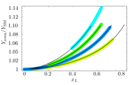
Figure 5: $X_{\rm even}/X_{\text{SM}}$ (left) and $Y_{\rm even}/Y_{\text{SM}}$ (right) as functions of $x_{L}$, for various values of $f=1,1.2,1.5$ and $2\,{\rm TeV}$ from top to bottom. The bands underlying the curves show the allowed ranges after applying electroweak precision constraints [30].

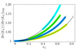
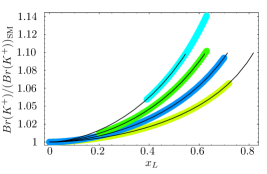
Figure 6: $Br(K_{L}\rightarrow\pi^{0}\nu\bar{\nu})/Br(K_{L}\rightarrow\pi^{0}\nu\bar{\nu})_{\text{SM}}$ (left) and $Br(K^{+}\rightarrow\pi^{+}\nu\bar{\nu})/Br(K^{+}\rightarrow\pi^{+}\nu\bar{\nu})_{\text{SM}}$ (right) in Scenario $1$, as functions of $x_{L}$ for different values of $f=1,1.2,1.5$ and $2\,{\rm TeV}$ from top to bottom. The bands underlying the curves show the allowed ranges after applying electroweak precision constraints [30].

In Fig. 5 we plot $X_{\rm even}/X_{\text{SM}}$ and $Y_{\rm even}/Y_{\text{SM}}$ as functions of $x_{L}$ for various values of $f$. We observe that the new physics contributions amount to modifications of the SM functions by at most $9\%$ and $14\%$, respectively, and of the corresponding rare decay branching ratios by at most $18\%$ and $28\%$. As an example we show in Fig. 6 $Br(K_{L}\rightarrow\pi^{0}\nu\bar{\nu})/Br(K_{L}\rightarrow\pi^{0}\nu\bar{\nu})_{\text{SM}}$ and $Br(K^{+}\rightarrow\pi^{+}\nu\bar{\nu})/Br(K^{+}\rightarrow\pi^{+}\nu\bar{\nu})_{\text{SM}}$ as functions of $x_{L}$ for different values of $f$. We observe that slightly larger effects can occur in $Br(K_{L}\rightarrow\pi^{0}\nu\bar{\nu})$ relative to $Br(K^{+}\rightarrow\pi^{+}\nu\bar{\nu})$.

10.3 Scenario 2

The new contributions to FCNC processes are in this scenario entirely dependent on only six parameters

$$x_{L}\,,\qquad f\,,\qquad m_{H1}\,,\qquad m_{H2}\,,\qquad m_{H3}\,,\qquad m_{H\ell}\,,$$ (10.4)

in addition to $m_{t}$ and the CKM parameters that we set to the central values obtained from tree level decays.

In spite of the fact that in this scenario $V_{Hd}=V_{\rm CKM}$, it does not belong to the class of MFV models. The point is that breaking the degeneracy of mirror fermion masses introduces a new source of flavour violation that has nothing to do with the top Yukawa couplings. Only if accidentally the contributions proportional to $\xi^{(q)}_{3}=\lambda_{t}^{(q)}$ dominate the new physics contributions, one would again end up with a scenario that effectively looks like MFV. However, as the mirror spectrum can be generally different from the quark spectrum and not as hierarchical as the latter one, the terms involving $\xi^{(q)}_{2}=\lambda_{c}^{(q)}$ in the formulae of the previous sections cannot be neglected, while this can be done in the T-even contributions. Moreover, as $\lambda_{c}^{(q)}$ are different from $\lambda_{t}^{(q)}$, that dominate the SM contributions, even in this simple scenario the usual MFV relations between $K$, $B_{d}$ and $B_{s}$ systems will be violated.

Specifically, for $q=d,s$, $\lambda_{c}^{(q)}$ are of the same order of magnitude as $\lambda_{t}^{(q)}$ and the MFV relations between $B_{d}$ and $B_{s}$ systems turn out to be only weakly violated. On the other hand, $\lambda_{c}^{(K)}/\lambda_{t}^{(K)}=\mathcal{O}(4\cdot 10^{2})$, implying that not only the MFV relations between $K$ and $B_{d,s}$ systems are strongly violated, but also the rate $Br(K^{+}\rightarrow\pi^{+}\nu\bar{\nu})$ can be significantly enhanced in this scenario, relative to the SM and Scenario $1$. In $Br(K^{+}\rightarrow\pi^{+}\nu\bar{\nu})$, in fact, the T-odd contribution proportional to ${\rm Re}(\lambda_{c}^{(K)})$ can have a significant effect, since ${\rm Re}(\lambda_{c}^{(K)})$ is much larger than ${\rm Im}(\lambda_{t}^{(K)})$ and ${\rm Re}(\lambda_{t}^{(K)})$. In $Br(K_{L}\rightarrow\pi^{0}\nu\bar{\nu})$, instead, only the imaginary part of the CKM contributions enters and, since ${\rm Im}(\lambda_{c}^{(K)})=-{\rm Im}(\lambda_{t}^{(K)})$, the T-odd contribution can only yield a slight suppression.

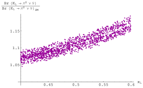
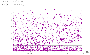
Figure 7: $Br(K_{L}\rightarrow\pi^{0}\nu\bar{\nu})/Br(K_{L}\rightarrow\pi^{0}\nu\bar{\nu})_{\text{SM}}$ (left) and $Br(K^{+}\rightarrow\pi^{+}\nu\bar{\nu})/Br(K^{+}\rightarrow\pi^{+}\nu\bar{\nu})_{\text{SM}}$ (right) in Scenario $2$, as functions of $x_{L}$, choosing $f=1\,{\rm TeV}$ and scanning over mirror fermion masses. The solid line in the right plot represents the SM prediction and separates the regions where $Br(K^{+}\rightarrow\pi^{+}\nu\bar{\nu})$ is suppressed or enhanced relative to the SM.

As an example, we show in Fig. 7 $Br(K_{L}\rightarrow\pi^{0}\nu\bar{\nu})/Br(K_{L}\rightarrow\pi^{0}\nu\bar{\nu})_{\text{SM}}$ and $Br(K^{+}\rightarrow\pi^{+}\nu\bar{\nu})/Br(K^{+}\rightarrow\pi^{+}\nu\bar{\nu})_{\text{SM}}$ as functions of $x_{L}$ , choosing $f=1\,{\rm TeV}$ and scanning over mirror fermion masses. We point out that the central values of the SM predictions appearing in the ratios shown in Fig. 7 differ from those quoted in (3.13) and read $Br(K^{+}\to\pi^{+}\nu\bar{\nu})=8.7\cdot 10^{-11}$, $Br(K_{L}\to\pi^{0}\nu\bar{\nu})=4.1\cdot 10^{-11}$. This difference comes from the CKM inputs that in the present analysis are taken from tree-level decays only. We observe that $Br(K_{L}\rightarrow\pi^{0}\nu\bar{\nu})$ can be enhanced at most by $17\%$ relative to the SM prediction, with stronger new physics effects at higher values of the $x_{L}$ parameter. In $Br(K^{+}\rightarrow\pi^{+}\nu\bar{\nu})$, instead, no clear dependence on the $x_{L}$ parameter can be seen, while larger (of a factor $5$) enhancements as well as suppressions of an order of magnitude can be obtained.

10.4 Breakdown of the Universality

In MFV models the functions $X_{i}$, $Y_{i}$ and $Z_{i}$ are independent of the index $i=K,d,s$. Consequently, they are universal quantities implying strong correlations between observables in $K$, $B_{d}$ and $B_{s}$ systems. The presence of mirror fermions in the LHT model generally breaks this universality, as we have already seen in Scenario $2$.

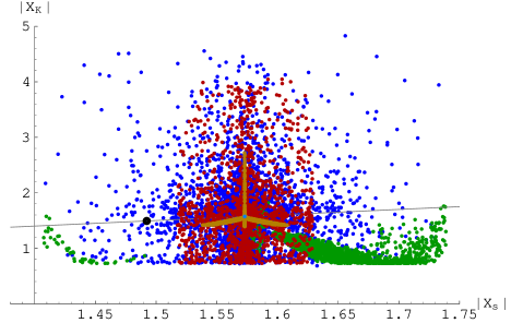
Figure 8: Breakdown of the universality between $|X_{K}|$ and $|X_{s}|$.

In Fig. 8 we show the ranges allowed in different scenarios in the space $(|X_{s}|,|X_{K}|)$. Here and in all the following plots, Scenarios $3$, $4$ and $6$ are represented by red, green and brown points, respectively, while blue points stand for the general scan. The solid line represents the MFV relation $|X_{s}|=|X_{K}|$, with the black point corresponding to the SM prediction $X_{\text{SM}}=1.49$ and the light blue point showing, for illustrative purposes, the Scenario $1$ result. The departure from the solid line gives the size of non-MFV contributions allowed in the various, differently coloured, scenarios. We observe that roughly

$$1.40\leq|X_{s}|\leq 1.75\,,\qquad 0.7\leq|X_{K}|\leq 4.7\,,$$ (10.5)

implying that the CP-conserving effects in the $K$ system can be much larger than in the $B_{s}$ system. A very similar behavior is found for the functions $Y_{i}$ and $Z_{i}$ with larger effects in the $K$ system relative to the $B_{d,s}$ systems. For instance

$$0.89\leq|Y_{s}|\leq 1.17\,,\qquad 0.41\leq|Y_{K}|\leq 3.9\,,$$ (10.6)

to be compared with $|Y_{s}|=|Y_{K}|=0.95$ in the SM.

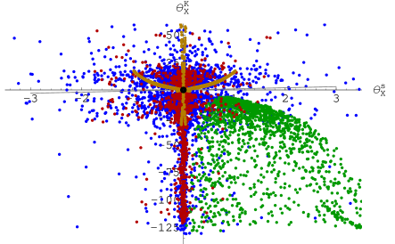
Figure 9: Breakdown of the universality between $\Theta_{X}^{K}$ and $\Theta_{X}^{s}$.

In Fig. 9, then, we show the allowed ranges in the space $(\Theta_{X}^{s},\Theta_{X}^{K})$, which roughly turn out to be

$$-3.5^{\circ}\leq\Theta_{X}^{s}\leq 3.5^{\circ}\,,\qquad-130^{\circ}\leq\Theta_{X}^{K}\leq 55^{\circ}\,,$$ (10.7)

implying that the CP–violating effects in the $b\to s$ transitions are tiny, while those in $K_{L}$ decays can be very large. An analogous pattern is found for the $Y_{s,K}$ and $Z_{s,K}$ functions. For the absolute values, the ranges in the $B_{d}$ and $B_{s}$ systems are similar, while in the $B_{d}$ system larger values for the phase ($\pm 13^{\circ}$) can be reached.

From the discussion of the previous plots it is evident that mirror fermion contributions break universality, and in a scenario-dependent way. Furthermore, we would like to stress and explain the origin of larger effects found in the $K$ system relative to the $B_{d,s}$ systems. Looking at the $X_{i}$ expression in (3.3) one sees that the mirror fermion contribution is enhanced by a factor $1/\lambda_{t}^{(i)}$. As $\lambda_{t}^{(K)}\simeq 4\cdot 10^{-4}$, whereas $\lambda_{t}^{(d)}\simeq 1\cdot 10^{-2}$ and $\lambda_{t}^{(s)}\simeq 4\cdot 10^{-2}$, we naively expect the deviation from $X_{\text{SM}}$ in the $K$ system to be by more than an order of magnitude larger than in the $B_{d}$ system, and even by two orders of magnitude larger than in the $B_{s}$ system. Analogous statements are valid for the $Y_{i}$ and $Z_{i}$ functions.

In view of the smallness of the new physics contributions in $b\to s$ transitions it is easy to satisfy the constraints from $B\to X_{s}\gamma$ and $B\to X_{s}\ell^{+}\ell^{-}$ that turn out to be close to the SM expectations. Therefore we will not further discuss them.

10.5 The $K\to\pi\nu\bar{\nu}$ System

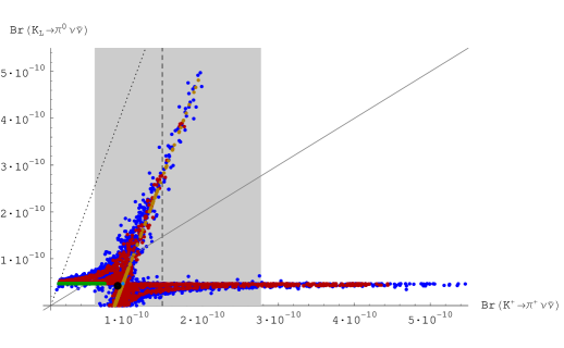
Figure 10: $Br(K_{L}\rightarrow\pi^{0}\nu\bar{\nu})$ as a function of $Br(K^{+}\rightarrow\pi^{+}\nu\bar{\nu})$. The shaded area represents the experimental $1\sigma$-range for $Br(K^{+}\rightarrow\pi^{+}\nu\bar{\nu})$. The GN-bound is displayed by the dotted line, while the solid line separates the two areas where $Br(K_{L}\rightarrow\pi^{0}\nu\bar{\nu})$ is larger or smaller than $Br(K^{+}\rightarrow\pi^{+}\nu\bar{\nu})$.

In Fig. 10 we show the correlation between $Br(K^{+}\rightarrow\pi^{+}\nu\bar{\nu})$ and $Br(K_{L}\rightarrow\pi^{0}\nu\bar{\nu})$ for the scenarios in question. The experimental $1\sigma$-range for $Br(K^{+}\rightarrow\pi^{+}\nu\bar{\nu})$ [52] and the model-independent Grossman-Nir (GN) bound [75] are also shown. We observe that even for the most general case, there are two branches of possible points. The first one is parallel to the GN-bound and leads to possible huge enhancements in $Br(K_{L}\rightarrow\pi^{0}\nu\bar{\nu})$ so that values as high as $5\cdot 10^{-10}$ are possible, being at the same time consistent with the measured value for $Br(K^{+}\rightarrow\pi^{+}\nu\bar{\nu})$. Within Scenario $6$ (brown points), this branch reduces to a straight line. The second branch corresponds to values for $Br(K_{L}\rightarrow\pi^{0}\nu\bar{\nu})$ being rather close to its SM prediction, while $Br(K^{+}\rightarrow\pi^{+}\nu\bar{\nu})$ is allowed to vary in the range $[1\cdot 10^{-11},5\cdot 10^{-10}]$, however, values above $4\cdot 10^{-10}$ are experimentally not favored. We note that within Scenario $4$ (green points), $Br(K_{L}\rightarrow\pi^{0}\nu\bar{\nu})$ is fixed to the T-even contribution and close to the SM value, and $Br(K^{+}\rightarrow\pi^{+}\nu\bar{\nu})$ is always smaller than in the SM so that the GN-bound can be reached.

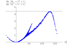
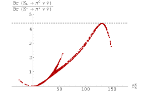
Figure 11: $Br(K_{L}\rightarrow\pi^{0}\nu\bar{\nu})/Br(K^{+}\rightarrow\pi^{+}\nu\bar{\nu})$ as a function of $\beta_{X}^{K}$, in the general scan and Scenarios $3$, $4$ and $6$, respectively. The dashed line represents the GN-bound.

In Fig. 11 we show the ratio $Br(K_{L}\rightarrow\pi^{0}\nu\bar{\nu})/Br(K^{+}\rightarrow\pi^{+}\nu\bar{\nu})$ as a function of the phase $\beta_{X}^{K}$, displaying again the GN-bound. We observe that the ratio can be significantly different from the SM prediction, with a possible enhancement of an order of magnitude. The two branches of Fig. 10 can be distinguished also here. In particular, points generated in Scenario $6$ appear only in the left branch and can not reach the GN-bound, while points belonging to Scenario $4$ populate the right branch and approach this bound.

The most interesting implications of this analysis are:

• If $Br(K^{+}\rightarrow\pi^{+}\nu\bar{\nu})$ is found sufficiently above the SM prediction but below $2.3\cdot 10^{-10}$, basically only two values for $Br(K_{L}\rightarrow\pi^{0}\nu\bar{\nu})$ are possible within the LHT model. One of these values is very close to the SM value in (3.13) and the second much larger.

• If $Br(K^{+}\rightarrow\pi^{+}\nu\bar{\nu})$ is found above $2.3\cdot 10^{-10}$, then only $Br(K_{L}\rightarrow\pi^{0}\nu\bar{\nu})$ with a value close to the SM one in (3.13) is possible.

• If $Br(K^{+}\rightarrow\pi^{+}\nu\bar{\nu})$ is found above the SM value, Scenario $4$ will be ruled out.

As Scenario $4$ was our favorite scenario in the analysis of $\Delta F=2$ processes in [33], with spectacular new physics effects in $S_{\psi\phi}$ and $A^{s}_{\rm SL}$ asymmetries, let us next have a closer look at the correlations between $S_{\psi\phi}$ and the $K\to\pi\nu\bar{\nu}$ decays.

10.6 $S_{\psi\phi}$ and $K\to\pi\nu\bar{\nu}$

In Figs. 12 and 13 we show the correlation between $S_{\psi\phi}$ and $Br(K_{L}\rightarrow\pi^{0}\nu\bar{\nu})$ and $Br(K^{+}\rightarrow\pi^{+}\nu\bar{\nu})$, respectively. We observe that in Scenario $4$ (green points), in which $S_{\psi\phi}$ can be significantly enhanced, $Br(K_{L}\rightarrow\pi^{0}\nu\bar{\nu})$ is very close to the SM value, while $Br(K^{+}\rightarrow\pi^{+}\nu\bar{\nu})$ is suppressed as already found previously. On the other hand in Scenario $6$ (brown points), both $Br(K_{L}\rightarrow\pi^{0}\nu\bar{\nu})$ and $Br(K^{+}\rightarrow\pi^{+}\nu\bar{\nu})$ can be strongly enhanced, while $S_{\psi\phi}$ is very close to the SM value. Only the general scan (blue points) can yield a simultaneous enhancement of these three observables. In order to see the triple correlation in question even better for all the scenarios, we show in Fig. 14 only those points of Fig. 10 for which $S_{\psi\phi}\geq 0.1$. It is evident that it is rather difficult to obtain simultaneously large values of the three observables in question. Still some sets of parameters belonging to the general scan exist for which this is possible.

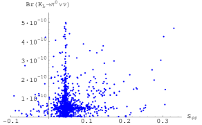
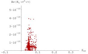
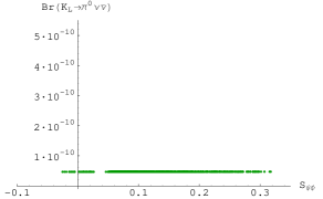
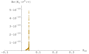
Figure 12: $Br(K_{L}\to\pi^{0}\nu\bar{\nu})$ as a function of $S_{\psi\phi}$, in the general scan and Scenarios $3$, $4$ and $6$, respectively.

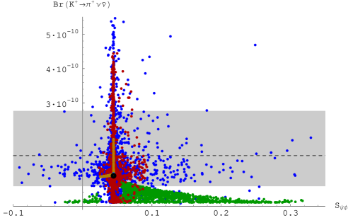
Figure 13: $Br(K^{+}\to\pi^{+}\nu\bar{\nu})$ as a function of $S_{\psi\phi}$. The shaded area represents the experimental $1\sigma$-range for $Br(K^{+}\rightarrow\pi^{+}\nu\bar{\nu})$.

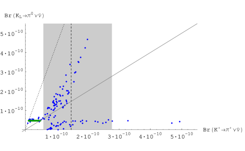
Figure 14: $Br(K_{L}\rightarrow\pi^{0}\nu\bar{\nu})$ as a function of $Br(K^{+}\rightarrow\pi^{+}\nu\bar{\nu})$, showing only the points that satisfy $S_{\psi\phi}\geq 0.1$. Like in Fig. 10, the shaded area represents the experimental $1\sigma$-range for $Br(K^{+}\rightarrow\pi^{+}\nu\bar{\nu})$, the GN-bound is displayed by the dotted line, while the solid line separates the two areas where $Br(K_{L}\rightarrow\pi^{0}\nu\bar{\nu})$ is larger or smaller than $Br(K^{+}\rightarrow\pi^{+}\nu\bar{\nu})$.

10.7 $B\to X_{s,d}\nu\bar{\nu}$

From the discussion of Section 10.4 we conclude that the branching ratios for the $B\to X_{s,d}\nu\bar{\nu}$ decays can be enhanced by at most $35\%$ over the SM predictions. Moreover, we find that

$$0.64\leq\left|\frac{X_{d}}{X_{s}}\right|^{2}\leq 1.56\,,$$ (10.8)

implying that the MFV relation between the ratio of the branching ratios in question and the CKM parameters given in (3.25) can be significantly violated.

10.8 $B_{d,s}\to\mu^{+}\mu^{-}$ versus $K\to\pi\nu\bar{\nu}$

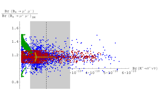
Figure 15: $Br(B_{s}\to\mu^{+}\mu^{-})/Br(B_{s}\to\mu^{+}\mu^{-})_{\text{SM}}$ as a function of $Br(K^{+}\rightarrow\pi^{+}\nu\bar{\nu})$. The shaded area represents the experimental $1\sigma$-range for $Br(K^{+}\rightarrow\pi^{+}\nu\bar{\nu})$ and the dark point shows the SM prediction.

We next investigate possible correlations between $B_{d,s}\to\mu^{+}\mu^{-}$ and $K\to\pi\nu\bar{\nu}$. In particular, we show in Fig. 15 the first correlation that will be accessible to future experiments: $Br(B_{s}\to\mu^{+}\mu^{-})/Br(B_{s}\to\mu^{+}\mu^{-})_{\text{SM}}$ as a function of $Br(K^{+}\rightarrow\pi^{+}\nu\bar{\nu})$. The experimental $1\sigma$-range for $Br(K^{+}\rightarrow\pi^{+}\nu\bar{\nu})$ [52] is represented by the shaded area and the SM prediction by the dark point. $Br(B_{s}\to\mu^{+}\mu^{-})$ can be about $50\%$ larger than in the SM, while more pronounced effects are possible in $Br(K^{+}\rightarrow\pi^{+}\nu\bar{\nu})$. Scenarios $4$ (green points) and $6$ (brown points) turn out to be again distinguishable through this correlation. As expected from our previous discussion, Scenario $4$ allows larger effects in the $B_{s}$ system, while Scenario $6$ is characterized by significant (of a factor $5$) enhancements in the $K$ system.

10.9 The $K_{L}\to\pi^{0}\ell^{+}\ell^{-}$ System

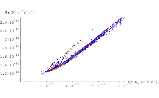
Figure 16: $Br(K_{L}\to\pi^{0}\mu^{+}\mu^{-})$ as a function of $Br(K_{L}\to\pi^{0}e^{+}e^{-})$.

In Fig. 16 we show the correlation between $Br(K_{L}\to\pi^{0}e^{+}e^{-})$ and $Br(K_{L}\to\pi^{0}\mu^{+}\mu^{-})$ that has been first investigated in [60, 61] in the framework of [37]. This correlation is only moderately sensitive to the scenario considered. We observe that both branching ratios can be enhanced up to a factor two, over the SM values (black point) in (8.11) and (8.12).

10.10 $K_{L}\to\pi^{0}\ell^{+}\ell^{-}$ versus $K_{L}\rightarrow\pi^{0}\nu\bar{\nu}$

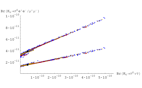
Figure 17: $Br(K_{L}\to\pi^{0}e^{+}e^{-})$ (upper curve) and $Br(K_{L}\to\pi^{0}\mu^{+}\mu^{-})$ (lower curve) as functions of $Br(K_{L}\rightarrow\pi^{0}\nu\bar{\nu})$. The corresponding SM predictions are represented by dark points.

In Fig. 17 we show $Br(K_{L}\to\pi^{0}e^{+}e^{-})$ and $Br(K_{L}\to\pi^{0}\mu^{+}\mu^{-})$ versus $Br(K_{L}\rightarrow\pi^{0}\nu\bar{\nu})$. We observe a strong correlation between $K_{L}\to\pi^{0}\ell^{+}\ell^{-}$ and $K_{L}\rightarrow\pi^{0}\nu\bar{\nu}$ decays that we expect to be valid beyond the LHT model, at least in models with the same operators present as in the SM. We note that a large enhancement of $Br(K_{L}\rightarrow\pi^{0}\nu\bar{\nu})$ automatically implies significant enhancements of $Br(K_{L}\to\pi^{0}\ell^{+}\ell^{-})$ and that different models and their parameter sets can than be distinguished by the position on the correlation curve. Moreover, measuring $Br(K_{L}\to\pi^{0}\ell^{+}\ell^{-})$ should allow a rather precise prediction of $Br(K_{L}\rightarrow\pi^{0}\nu\bar{\nu})$ at least in models with the same operators as the SM.

10.11 Violation of Golden MFV Relations

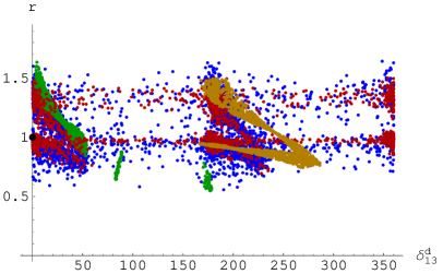
Figure 18: The ratio $r$ as a function of $\delta_{13}^{d}$.

In Fig. 18 we show the ratio $r$ of (3.20) as a function of $\delta_{13}^{d}$. Its departure from unity measures the violation of the golden MFV relation between $B_{d,s}\to\mu^{+}\mu^{-}$ decays and $\Delta M_{d,s}$ in (3.20). We observe that $r$ can vary in the range

$$0.6\leq r\leq 1.7\,,$$ (10.9)

with, as expected, Scenario $4$ (green points) able to achieve these bounding values more easily than Scenarios $3$ (red points) and $6$ (brown points). Such departures from unity could easily be tested in view of a theoretically clean character of (3.20).

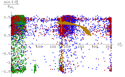
Figure 19: $\sin 2\beta_{X}^{K}/\sin(2\beta+2\varphi_{B_{d}})$ as a function of $\delta^{d}_{13}$.

Furthermore, in Fig. 19 we show the ratio of $\sin 2\beta_{X}^{K}$ over $\sin(2\beta+2\varphi_{B_{d}})$ as a function of $\delta_{13}^{d}$ for the scenarios considered. Similarly to $r$, the departure of this ratio from unity measures the violation of a golden MFV relation (3.11), this time between the CP-violating phases in the $K\to\pi\nu\bar{\nu}$ system and in the $B_{d}^{0}-\bar{B}^{0}_{d}$ mixing. As $\varphi_{B_{d}}$ is constrained by the measured $S_{\psi K_{S}}$ asymmetry to be at most a few degrees [40, 68], large violations of the relation in question can only follow from the $K\to\pi\nu\bar{\nu}$ decays. As seen in Fig. 19, they can be spectacular.

10.12 The dependence on $\delta^{d}_{13}$

As seen in Figs. 18 and 19 there are two oases in the values of $\delta^{d}_{13}$

$$-10^{\circ}\leq\delta^{d}_{13}\leq 50^{\circ},\qquad 170^{\circ}\leq\delta^{d}_{13}\leq 250^{\circ},$$ (10.10)

with the desert between the two oases visibly but not densely populated. The origin of the oases is the constraint from $S_{\psi K_{S}}$. It is interesting to observe again a clear separation between Scenarios 4 and 6. While in Scenario 4 (green points) the first oasis is dominantly populated, in Scenario 6 (brown points) the second oasis is occupied. Moreover in the latter case there is an interesting excursion of points into the desert up to $\delta_{13}^{d}=290^{\circ}$. The desert, instead, in which large effects simultaneously in $K$ and $B$ systems can be found, is dominated by red and blue points corresponding to Scenario 3 and the general scan, respectively.

10.13 Comparison of Various Scenarios

The plots in Figs. 10-19 are self-explanatory. Yet, we would like to make a few general observations:

• There is a very clear distinction between scenarios $4$ and $6$. Scenario $4$ can be considered as “$B_{s}$–scenario” as it gives interesting effects in the $B_{s}$ system.

• On the other hand Scenario $6$ can be considered as “$K$–scenario” as it admits spectacular effects in $K$ decays.

• Moreover, for certain sets of the LHT parameters obtained in the general scan, large departures from the SM predictions in $K$ and $B_{d,s}$ decays can be simultaneously found.

10.14 $B\to\pi K$ Decays in the LHT Model

We have finally investigated the impact of new physics contributions on $B\to\pi K$ decays that, for some time, signaled the presence of enhanced electroweak penguin contributions with new large CP-violating phases. In a simple new physics scenario in which the universality between $b\bar{s}$-penguins relevant for $B\to\pi K$ and $s\bar{d}$-penguins relevant for $K\to\pi\nu\bar{\nu}$ has been assumed [37], the enhanced electroweak penguins required to fit the $B\to\pi K$ data implied spectacular effects in the $K\to\pi\nu\bar{\nu}$ system, similar to those shown in Figs. 10-12.

Meanwhile, the data on $B\to\pi K$ decays significantly changed [76, 77, 78] so that the SM predictions for the so-called $R_{n}$ and $R_{c}$ ratios [37] are nowadays within one standard deviations from the data. Consequently, within the new physics scenario of [37] no large effects in $K\to\pi\nu\bar{\nu}$ are expected.

The picture is quite different in the LHT model, where the universality between $b\bar{s}$ and $s\bar{d}$ systems can be strongly broken. Following the approach of [37] to determine the hadronic parameters of the $B\to\pi K$ system from the $B\to\pi\pi$ data and calculating the electroweak penguin contributions to $B\to\pi K$ decays in the LHT model, we find that the new physics effects in these rare decays are smaller than the theoretical uncertainties present in non-leptonic decays. These small effects follow primarily from the smallness of complex phases in the $b\bar{s}$ penguins as given in (10.7) to be compared with $\pm 90^{\circ}$ taken in past $B\to\pi K$ analyses.

In summary, in the LHT model the smallness of new physics in $B\to\pi K$ decays does not imply its smallness in $K\to\pi\nu\bar{\nu}$ decays as seen in Figs 10-14.

10.15 What if the $\sin 2\beta$ problem disappears?

Until now, our analysis was based on the tree level determination of the angle $\beta$ that, due to the high value of $R_{b}$, is larger than the one measured through the $S_{\psi K_{S}}$ asymmetry. It is conceivable that future tree level determinations of $R_{b}$ will yield lower values for $R_{b}$ and consequently for $\beta$, so that the $\sin 2\beta$ problem will disappear. We have repeated the whole analysis for such a scenario, finding that the $\sin 2\beta$ problem has a very minor impact on our analysis, in particular in $B_{s}$ and $K$ decays. For instance, large effects in $K\to\pi\nu\bar{\nu}$ decays and simultaneously in $S_{\psi\phi}$ can still be found.

10.16 What if the $B_{d}$ and $B_{s}$ Decays are SM-like?

Finally, we can consider a very pessimistic scenario where BaBar, Belle and LHC will confirm all the SM expectations in $B_{d}$ and $B_{s}$ decays, finding in particular both the $S_{\psi K_{S}}$ and $S_{\psi\phi}$ asymmetries very close to the SM values. This could already happen at the end of this decade. The question then arises whether in such a situation we could still expect large departures from the SM values in rare $K$ decays, whose precise measurements will be available only in the next decade. It is evident from Figs. 10-14 that even in this, pessimistic for $B$-physics, scenario, spectacular effects in $K\to\pi\nu\bar{\nu}$ and also large effects in $K_{L}\to\pi^{0}\ell^{+}\ell^{-}$ will be possible in particular in Scenario 6.

11 Summary and Outlook

In this paper we have analyzed for the first time rare $K$ and $B$ decays in the Littlest Higgs model with T-parity [14, 15, 16, 29]. Together with our previous work [33] on observables related to particle-antiparticle mixing and $B\to X_{s,d}\gamma$, the results of the present paper allow us to obtain a general description of FCNC processes in this model.

On the technical side, we have presented a complete set of Feynman rules for the LHT model including also vertices with Goldstone bosons. The inclusion of $\mathcal{O}(v^{2}/f^{2})$ corrections to some of the vertices has been performed here for the first time. These Feynman rules allow the calculations of $\mathcal{O}(v^{2}/f^{2})$ contributions in arbitrary gauge and should turn out to be useful also for other observables.

Using these rules we have calculated in the LHT model the short distance functions $X_{i}$, $Y_{i}$ and $Z_{i}$ ($i=K,d,s$). In the LHT model these functions are complex quantities and carry the index $i$ to signal the breakdown of the universality of FCNC processes, valid in the SM. The new weak phases in $X_{i}$, $Y_{i}$ and $Z_{i}$, which are absent in the SM and models with MFV, imply potential new CP-violating effects beyond the SM ones. We would like to emphasize that the new parameterization of rare decays in terms of non-universal functions $X_{i}$, $Y_{i}$ and $Z_{i}$ can be applied to any model with new flavour and CP-violating interactions but the same low energy operators.

With the functions $X_{i}$, $Y_{i}$ and $Z_{i}$ at hand, one can straightforwardly calculate the branching ratios for a number of interesting rare decays. In particular, we analyzed $K^{+}\to\pi^{+}\nu\bar{\nu}$, $K_{L}\to\pi^{0}\nu\bar{\nu}$, $B_{s,d}\to\mu^{+}\mu^{-}$, $B\to X_{s,d}\nu\bar{\nu}$, $B\to X_{s}\ell^{+}\ell^{-}$, $K_{L}\to\pi^{0}\ell^{+}\ell^{-}$ and $B\to\pi K$. At all stages of our numerical analysis we took into account the existing constraints from electroweak precision studies [30] and from particle-antiparticle mixing and $B\to X_{s}\gamma$ studied by us in [33] and from $B\to X_{s}\ell^{+}\ell^{-}$ calculated here.

The main messages of our paper are as follows:

• The most evident departures from the SM predictions are found for CP-violating observables that are strongly suppressed within this model. These are the branching ratio for $K_{L}\to\pi^{0}\nu\bar{\nu}$ and the CP-asymmetry $S_{\psi\phi}$.

• Large departures from SM expectations are also possible for $Br(K_{L}\to\pi^{0}\ell^{+}\ell^{-})$ and $Br(K^{+}\to\pi^{+}\nu\bar{\nu})$.

• The branching ratios for $B_{s,d}\to\mu^{+}\mu^{-}$ and $B\to X_{s,d}\nu\bar{\nu}$, instead, are modified by at most $50\%$ and $35\%$, respectively, and the effects of new electroweak penguins in $B\to\pi K$ are small, in agreement with the recent data.

• Sizable departures from MFV relations between $\Delta M_{s,d}$ and $Br(B_{s,d}\to\mu^{+}\mu^{-})$ and between $S_{\psi K_{S}}$ and the $K\to\pi\nu\bar{\nu}$ decay rates are possible.

• The universality of new physics effects, characteristic for MFV models, can be largely broken, in particular between $K$ and $B_{s,d}$ systems.

• The new physics effects in $B\to X_{s,d}\gamma$ and $B\to X_{s,d}\ell^{+}\ell^{-}$ turn out to be below $5\%$ and $15\%$, respectively so that agreement with the data can easily be obtained.

One of the important findings of our paper is the presence of left-over singularities in the mirror sector that signals some sensitivity of the final results to the UV completion of the theory. This issue has been discussed in detail in the context of the LH model without T-parity in [28], is known from the study of electroweak constraints [29] and has been considered in Section 6 of the present paper. In estimating the contribution of these logarithmic singularities, we have assumed the UV completion of the theory not to have a complicate flavour pattern or at least that it has no impact below the cut-off. Clearly, this additional assumption lowers the predictive power of the theory. In spite of that, we believe that the general picture of FCNC processes presented here and in our previous paper is only insignificantly shadowed by this general property of non-linear sigma models.

We conclude with probably one of the most important messages of this paper and of our previous analysis:

• In spite of an impressive agreement of the SM with the available data, large departures from the SM expectations in $B_{s}$ decays are still possible. However, even if future Tevatron and LHC data would not see any significant new physics effect in these decays, this will not imply necessarily that new physics is not visible in $K_{L}\rightarrow\pi^{0}\nu\bar{\nu}$, $K^{+}\rightarrow\pi^{+}\nu\bar{\nu}$ and $K_{L}\to\pi^{0}\ell^{+}\ell^{-}$. On the contrary, as seen in the case of Scenario $6$, large departures in these three decays will still be possible. It may then be that in the end, it will be $K$ physics and not $B$ physics that will offer the best information about the new phenomena at very short distance scales, in accordance with the arguments in [79, 80].

Acknowledgements

We would like to thank Björn Duling for checking the Feynman rules given in Appendix B and William A. Bardeen, Ulrich Haisch and Kazuhiro Tobe for useful discussions. This research was partially supported by the German ‘Bundesministerium für Bildung und Forschung’ under contracts 05HT4WOA/3, 05HT6WOA.

Appendix A Non-leading contributions of $\bm{\Phi}$

In this Appendix we show that the scalar triplet $\Phi$ does not contribute to the decays considered in the present paper at ${\cal O}(v^{2}/f^{2})$.

In principle, also the scalar triplet $\Phi$ could contribute to the decays considered in the present analysis. The corresponding diagrams can be obtained from the ones shown in Figs. 1 and 2 by simply replacing $W^{\pm}_{H}$ by $\phi^{\pm}$ and $Z_{H},\,A_{H}$ by $\phi^{0},\,\phi^{P}$. Therefore we also derived the Feynman rules for the vertices containing $\Phi$. We found them to have the following generic structure:

$$\bar{q}_{H}\Phi q\sim c\frac{m^{q}_{H}}{M_{\Phi}}\frac{v^{2}}{f^{2}}P_{L}-c^{\prime}\frac{m_{q}}{M_{\Phi}}P_{R}\,,\qquad\Phi G_{H}G_{L}\sim{\cal O}\left(\frac{v^{2}}{f}\right)\,,$$ (A.1)

where $c,\,c^{\prime}$ are ${\cal O}(1)$ coefficients depending on which $q_{H}$, $q$ and component of $\Phi$ are involved, and $P_{R,L}=(1\pm\gamma_{5})/2$ are the usual projectors. $q_{H}$ and $q$ denote mirror and SM fermions, respectively, and $G_{H},\,G_{L}$ are heavy and light gauge bosons.

As we have set the masses of the external quarks and leptons to zero throughout our analysis, we obtain

$$\bar{q}_{H}\Phi q\sim{\cal O}\left(\frac{v^{2}}{f^{2}}\right)\qquad\text{and}\qquad\Phi G_{H}G_{L}\sim{\cal O}\left(\frac{v^{2}}{f}\right)\,.$$ (A.2)

It can now be easily seen that each diagram contains at least two such vertices, so that they are suppressed by ${\cal O}(v^{4}/f^{4})$.

Furthermore, in contrast to the LH model without T-parity, all particles running in the loops have ${\cal O}(f)$ masses, so that no cancellation of $v/f$ factors due to large mass ratios, as encountered in [26, 28] for diagrams with $T_{+}$ exchanges, can appear.

Thus we find that $\Phi$ contributes to the decays in question – and more in general to all decays with external SM fermions – only at ${\cal O}(v^{4}/f^{4})$. For this reason we do not give any Feynman rule for the interactions of the scalar triplet $\Phi$.

Appendix B Relevant Feynman Rules

In this Appendix we list all Feynman rules relevant for the analysis performed in the present paper, and describe briefly how they have been derived. We note that given the Feynman rule for a vertex, the rule for the conjugate one can be obtained through the replacement (vertex)$\rightarrow-$(vertex)^†. There follow, in particular, the prescriptions $P_{L}\rightarrow-P_{R}$, $P_{R}\rightarrow-P_{L}$ and $\gamma_{\mu}P_{L,R}\rightarrow\gamma_{\mu}P_{L,R}$. A similar, but more detailed description for the LH model without T-parity can be found in [17] and in [24, 28], where some of the Feynman rules given in [17] have been corrected.

B.1 Fermion–Gauge Boson Couplings

The fermion–gauge boson couplings can easily be obtained from the fermion kinetic term [41]

$$\mathcal{L}_{\text{fermion}}=\bar{\Psi}_{1}\bar{\sigma}^{\mu}D^{1}_{\mu}\Psi_{1}+\bar{\Psi}_{2}\bar{\sigma}^{\mu}D^{2}_{\mu}\Psi_{2}+\bar{t}_{1}^{\prime}\bar{\sigma}^{\mu}D^{\prime 1}_{\mu}t_{1}^{\prime}+\bar{t}_{2}^{\prime}\bar{\sigma}^{\mu}D^{\prime 2}_{\mu}t_{2}^{\prime}\,,$$ (B.1)

where

$$D^{1}_{\mu} = \partial_{\mu}-\sqrt{2}igQ_{1}^{a}W_{1\mu}^{a}-\sqrt{2}ig^{\prime}Y_{1}^{(\Psi_{1})}B_{1\mu}-\sqrt{2}ig^{\prime}Y_{2}^{(\Psi_{1})}B_{2\mu}\,,$$ (B.2)

$$D^{2}_{\mu} = \partial_{\mu}+\sqrt{2}igQ_{2}^{aT}W_{2\mu}^{a}-\sqrt{2}ig^{\prime}Y_{1}^{(\Psi_{2})}B_{1\mu}-\sqrt{2}ig^{\prime}Y_{2}^{(\Psi_{2})}B_{2\mu}\,,$$ (B.3)

$$D^{\prime i}_{\mu} = \partial_{\mu}-\sqrt{2}ig^{\prime}Y_{1}^{(t^{\prime}_{i})}B_{1\mu}-\sqrt{2}ig^{\prime}Y_{2}^{(t^{\prime}_{i})}B_{2\mu}\,,$$ (B.4)

by inserting the mass eigenstates of all particles involved. The $U(1)$ charges can be obtained from gauge invariance of the Yukawa couplings and T-parity [41] and are given in Table 2.

$q_{1}$	$(1/30,2/15)$	$q_{2}$	$(2/15,1/30)$
$t^{\prime}_{1}$	$(8/15,2/15)$	$t^{\prime}_{2}$	$(2/15,8/15)$
$t^{\prime}_{1R}$	$(8/15,2/15)$	$t^{\prime}_{2R}$	$(2/15,8/15)$
$u_{R}$	$(1/3,1/3)$	$d_{R}$	$(-1/6,-1/6)$
$\ell_{1}$	$(-1/5,-3/10)$	$\ell_{2}$	$(-3/10,-1/5)$
$e_{R}$	$(-1/2,-1/2)$

Table 2: $U(1)_{1}\times U(1)_{2}$ quantum numbers of the fermion fields.

Similar kinetic terms can be written down for the right-handed SM fields and for $t^{\prime}_{iR},\;i=1,2$.

The kinetic term for the right-handed mirror fermions can be written down by using the CCWZ approach [31, 81] and is given in explicit terms in [41]. As the mirror fermions are purely vector-like under $SU(2)_{L}\times U(1)_{Y}$, their couplings to SM gauge bosons are proportional to $\gamma^{\mu}$. Thus there is no need to consider the CCWZ kinetic term any further, as the couplings of the right-handed mirror fermions to SM gauge bosons have to be equal to the ones of the left-handed mirror fermions.

Fermion couplings to SM gauge bosons
$\bar{f}A_{L}f$	$ieQ_{f}\gamma^{\mu}$
$\bar{u}^{i}Z_{L}u^{i}$	$\frac{ig}{\cos{\theta_{W}}}\gamma^{\mu}\left[\left(\frac{1}{2}-\frac{2}{3}\sin^{2}{\theta_{W}}\right)P_{L}-\frac{2}{3}\sin^{2}{\theta_{W}}P_{R}\right]$
$\bar{d}^{i}Z_{L}d^{i}$	$\frac{ig}{\cos{\theta_{W}}}\gamma^{\mu}\left[\left(-\frac{1}{2}+\frac{1}{3}\sin^{2}{\theta_{W}}\right)P_{L}+\frac{1}{3}\sin^{2}{\theta_{W}}P_{R}\right]$
$\bar{t}Z_{L}t$	$\frac{ig}{\cos{\theta_{W}}}\gamma^{\mu}\left[\left(\frac{1}{2}\left(1-x_{L}^{2}\frac{v^{2}}{f^{2}}\right)-\frac{2}{3}\sin^{2}{\theta_{W}}\right)P_{L}-\frac{2}{3}\sin^{2}{\theta_{W}}P_{R}\right]$
$\bar{T}_{+}Z_{L}T_{+}$	$\frac{ig}{\cos{\theta_{W}}}\gamma^{\mu}\left[\left(\frac{1}{2}x_{L}^{2}\frac{v^{2}}{f^{2}}-\frac{2}{3}\sin^{2}{\theta_{W}}\right)P_{L}-\frac{2}{3}\sin^{2}{\theta_{W}}P_{R}\right]$
$\bar{T}_{+}Z_{L}t$	$\frac{ig}{\cos{\theta_{W}}}\frac{x_{L}}{2}\frac{v}{f}\left[1+\frac{v^{2}}{f^{2}}\left(d_{2}-\frac{x_{L}^{2}}{2}\right)\right]\gamma^{\mu}P_{L}$
$\bar{u}^{i}_{H}Z_{L}u^{i}_{H}$	$\frac{ig}{\cos{\theta_{W}}}\left[\left(\frac{1}{2}-\frac{2}{3}\sin^{2}{\theta_{W}}\right)\right]\gamma^{\mu}$
$\bar{d}^{i}_{H}Z_{L}d^{i}_{H}$	$\frac{ig}{\cos{\theta_{W}}}\left[\left(-\frac{1}{2}+\frac{1}{3}\sin^{2}{\theta_{W}}\right)\right]\gamma^{\mu}$
$\bar{T}_{-}Z_{L}T_{-}$	$-\frac{2ig}{3\cos{\theta_{W}}}\sin^{2}{\theta_{W}}\gamma^{\mu}$
$\bar{u}^{i}W^{+\mu}_{L}d^{j}$	$\frac{ig}{\sqrt{2}}(V_{\text{CKM}})_{ij}\gamma^{\mu}P_{L}$
$\bar{t}W^{+\mu}_{L}d^{j}$	$\frac{ig}{\sqrt{2}}(V_{\text{CKM}})_{tj}\left(1-\frac{x_{L}^{2}}{2}\frac{v^{2}}{f^{2}}\right)\gamma^{\mu}P_{L}$
$\bar{T}_{+}W^{+\mu}_{L}d^{j}$	$\frac{ig}{\sqrt{2}}(V_{\text{CKM}})_{tj}x_{L}\frac{v}{f}\left(1+\frac{v^{2}}{f^{2}}d_{2}\right)\gamma^{\mu}P_{L}$
$\bar{u}^{i}_{H}W^{+\mu}_{L}d^{j}_{H}$	$\frac{ig}{\sqrt{2}}\delta_{ij}\gamma^{\mu}$
$\bar{\nu}^{i}Z_{L}\nu^{i}$	$\frac{ig}{2\cos{\theta_{W}}}\gamma^{\mu}P_{L}$
$\bar{\ell}^{i}Z_{L}\ell^{i}$	$\frac{ig}{\cos{\theta_{W}}}\gamma^{\mu}\left[\left(-\frac{1}{2}+\sin^{2}{\theta_{W}}\right)P_{L}+\sin^{2}{\theta_{W}}P_{R}\right]$
$\bar{\nu}^{i}_{H}Z_{L}\nu^{i}_{H}$	$\frac{ig}{2\cos{\theta_{W}}}\gamma^{\mu}$
$\bar{\ell}^{i}_{H}Z_{L}\ell^{i}_{H}$	$\frac{ig}{\cos{\theta_{W}}}\left[\left(-\frac{1}{2}+\sin^{2}{\theta_{W}}\right)\right]\gamma^{\mu}$
$\bar{\nu}^{i}W^{+\mu}_{L}\ell^{j}$	$\frac{ig}{\sqrt{2}}(V_{\text{PMNS}})_{ij}\gamma^{\mu}P_{L}$
$\bar{\nu}^{i}_{H}W^{+\mu}_{L}\ell^{j}_{H}$	$\frac{ig}{\sqrt{2}}\delta_{ij}\gamma^{\mu}$

The couplings to the heavy gauge bosons have already been given in [32]. We confirm the findings of these authors, and include also $v^{2}/f^{2}$ corrections to the couplings of the neutral gauge bosons. These corrections turn out to be irrelevant in the decays considered in the present paper, but could be of relevance for other processes. While our paper was being completed, the rules for the quark sector appeared also in [42], but without performing the $v/f-$ expansion and without taking into account the flavour mixing matrices $V_{Hu}$ and $V_{Hd}$.

Note that the couplings to the heavy gauge bosons are purely left-handed as there is no kinetic term including both heavy and light right-handed fermions. The only exception are the couplings involving $T_{-}$ together with $T_{+}$ or $t$.

Fermion couplings to heavy gauge bosons
$\bar{u}^{i}_{H}A_{H}u^{j}$	$\left(-\frac{ig^{\prime}}{10}-\frac{ig}{2}x_{H}\frac{v^{2}}{f^{2}}\right)(V_{Hu})_{ij}\gamma^{\mu}P_{L}$
$\bar{u}^{i}_{H}Z_{H}u^{j}$	$\left(\frac{ig}{2}-\frac{ig^{\prime}}{10}x_{H}\frac{v^{2}}{f^{2}}\right)(V_{Hu})_{ij}\gamma^{\mu}P_{L}$
$\bar{d}^{i}_{H}A_{H}d^{j}$	$\left(-\frac{ig^{\prime}}{10}+\frac{ig}{2}x_{H}\frac{v^{2}}{f^{2}}\right)(V_{Hd})_{ij}\gamma^{\mu}P_{L}$
$\bar{d}^{i}_{H}Z_{H}d^{j}$	$\left(-\frac{ig}{2}-\frac{ig^{\prime}}{10}x_{H}\frac{v^{2}}{f^{2}}\right)(V_{Hd})_{ij}\gamma^{\mu}P_{L}$
$\bar{u}^{i}_{H}A_{H}t$	$\left[-\frac{ig^{\prime}}{10}+\left(\frac{ig^{\prime}}{20}{x_{L}^{2}}-\frac{ig}{2}x_{H}\right)\frac{v^{2}}{f^{2}}\right](V_{Hu})_{i3}\gamma^{\mu}P_{L}$
$\bar{u}^{i}_{H}Z_{H}t$	$\left[\frac{ig}{2}-\left(\frac{ig}{4}x_{L}^{2}+\frac{ig^{\prime}}{10}x_{H}\right)\frac{v^{2}}{f^{2}}\right](V_{Hu})_{i3}\gamma^{\mu}P_{L}$
$\bar{u}^{i}_{H}A_{H}T_{+}$	$-\frac{ig^{\prime}}{10}x_{L}\frac{v}{f}(V_{Hu})_{i3}\gamma^{\mu}P_{L}$
$\bar{u}^{i}_{H}Z_{H}T_{+}$	$\frac{ig}{2}x_{L}\frac{v}{f}(V_{Hu})_{i3}\gamma^{\mu}P_{L}$
$\bar{T}_{-}A_{H}t$	$-\frac{2}{5}ig^{\prime}\gamma^{\mu}\left(x_{L}\frac{v}{f}P_{L}+\sqrt{x_{L}}\left(1-\frac{v^{2}}{f^{2}}(1-x_{L})(\frac{1}{2}-x_{L})\right)P_{R}\right)$
$\bar{T}_{-}Z_{H}t$	$-\frac{2}{5}ig^{\prime}x_{H}\sqrt{x_{L}}\frac{v^{2}}{f^{2}}\gamma^{\mu}P_{R}$
$\bar{T}_{-}A_{H}T_{+}$	$\frac{2}{5}ig^{\prime}\gamma^{\mu}\left[\left(1-\frac{x_{L}^{2}}{2}\frac{v^{2}}{f^{2}}\right)P_{L}+\sqrt{1-x_{L}}\left(1+\frac{v^{2}}{f^{2}}x_{L}(\frac{1}{2}-x_{L})\right)P_{R}\right]$
$\bar{T}_{-}Z_{H}T_{+}$	$\frac{2}{5}ig^{\prime}x_{H}\frac{v^{2}}{f^{2}}\gamma^{\mu}(P_{L}+\sqrt{1-x_{L}}P_{R})$
$\bar{u}^{i}_{H}W^{+\mu}_{H}d^{j}$	$\frac{ig}{\sqrt{2}}(V_{Hd})_{ij}\gamma^{\mu}P_{L}$
$\bar{d}^{i}_{H}W^{-\mu}_{H}u^{j}$	$\frac{ig}{\sqrt{2}}(V_{Hu})_{ij}\gamma^{\mu}P_{L}$
$\bar{d}^{i}_{H}W^{-\mu}_{H}t$	$\frac{ig}{\sqrt{2}}(V_{Hu})_{i3}\left(1-\frac{x_{L}^{2}}{2}\frac{v^{2}}{f^{2}}\right)\gamma^{\mu}P_{L}$
$\bar{d}^{i}_{H}W^{-\mu}_{H}T_{+}$	$\frac{ig}{\sqrt{2}}(V_{Hu})_{i3}x_{L}\frac{v}{f}\gamma^{\mu}P_{L}$
$\bar{\nu}^{i}_{H}A_{H}\nu^{j}$	$\left(\frac{ig^{\prime}}{10}-\frac{ig}{2}x_{H}\frac{v^{2}}{f^{2}}\right)(V_{H\nu})_{ij}\gamma^{\mu}P_{L}$
$\bar{\nu}^{i}_{H}Z_{H}\nu^{j}$	$\left(\frac{ig}{2}+\frac{ig^{\prime}}{10}x_{H}\frac{v^{2}}{f^{2}}\right)(V_{H\nu})_{ij}\gamma^{\mu}P_{L}$
$\bar{\ell}^{i}_{H}A_{H}\ell^{j}$	$\left(\frac{ig^{\prime}}{10}+\frac{ig}{2}x_{H}\frac{v^{2}}{f^{2}}\right)(V_{H\ell})_{ij}\gamma^{\mu}P_{L}$
$\bar{\ell}^{i}_{H}Z_{H}\ell^{j}$	$\left(-\frac{ig}{2}+\frac{ig^{\prime}}{10}x_{H}\frac{v^{2}}{f^{2}}\right)(V_{H\ell})_{ij}\gamma^{\mu}P_{L}$
$\bar{\nu}^{i}_{H}W^{+\mu}_{H}\ell^{j}$	$\frac{ig}{\sqrt{2}}(V_{H\ell})_{ij}\gamma^{\mu}P_{L}$
$\bar{\ell}^{i}_{H}W^{-\mu}_{H}\nu^{j}$	$\frac{ig}{\sqrt{2}}(V_{H\nu})_{ij}\gamma^{\mu}P_{L}$

B.2 Fermion–Goldstone Boson Couplings

The fermion couplings to T-even and T-odd Goldstone bosons can be derived from the Yukawa interactions (2.23), (2.38) and (2.40) and from the mass term (2.20). Note that (2.40) with $X=(\Sigma_{33})^{-1/4}$ corresponds to case A in [43]. Using instead $X=(\Sigma_{33}^{\dagger})^{1/4}$ (case B in [43]) does not modify the fermion couplings to Goldstone bosons as required by gauge invariance.

As these terms have again to be expressed in mass eigenstates of the particles involved, we have to take into account the ${\cal O}(v^{2}/f^{2})$ mixing of the Goldstone bosons and scalars [30]. Following the steps of [30], we find the mass eigenstates, denoted here with a subscript “$m$”, to be

$$\pi^{0}_{m} = \pi^{0}\left(1-\frac{v^{2}}{12f^{2}}\right)\,,$$ (B.5)

$$\pi^{\pm}_{m} = \pi^{\pm}\left(1-\frac{v^{2}}{12f^{2}}\right)\,,$$ (B.6)

$$h_{m} = h\,,$$ (B.7)

$$\phi^{0}_{m} = \phi^{0}\left(1-\frac{v^{2}}{12f^{2}}\right)\,,$$ (B.8)

$$\phi^{P}_{m} = \phi^{P}-\left(\sqrt{10}\eta-\sqrt{2}\omega^{0}+\phi^{P}\right)\frac{v^{2}}{12f^{2}}\,,$$ (B.9)

$$\phi^{\pm}_{m} = \phi^{\pm}\left(1-\frac{v^{2}}{24f^{2}}\right)\mp i\omega^{\pm}\frac{v^{2}}{12f^{2}}\,,$$ (B.10)

$$\phi^{++}_{m} = \phi^{++}\,,$$ (B.11)

$$\eta_{m} = \eta-\frac{5g^{\prime}\eta-4\sqrt{5}[g^{\prime}(\omega^{0}+\sqrt{2}\phi^{P})-6gx_{H}\omega^{0}]}{24g^{\prime}}\frac{v^{2}}{f^{2}}\,,$$ (B.12)

$$\omega^{0}_{m} = \omega^{0}-\frac{5g(\omega^{0}+4\sqrt{2}\phi^{P})-4\sqrt{5}\eta(5g+6g^{\prime}x_{H})}{120g}\frac{v^{2}}{f^{2}}\,,$$ (B.13)

$$\omega^{\pm}_{m} = \omega^{\pm}\left(1-\frac{v^{2}}{24f^{2}}\right)\mp\frac{i}{6}\phi^{\pm}\frac{v^{2}}{f^{2}}\,.$$ (B.14)

In what follows, we will drop the subscript “$m$”, as it is clear that all Feynman rules are given in terms of mass eigenstates.

Note that the mixing of Goldstone bosons and scalars in question affect the corresponding Feynman rules at ${\cal O}(v^{2}/f^{2})$, thus without considering it, one would not be able to get the right ${\cal O}(v^{2}/f^{2})$ corrections. Also the ${\cal O}(v^{2}/f^{2})$ corrections to the particle masses have to be taken into account.

We would like to caution the reader that this mixing has not been taken into account in the derivation of the Feynman rules for $\Phi$ given in [41].

Fermion couplings to SM Goldstone bosons
$\bar{u}^{i}\pi^{+}d^{j}$	$\frac{g}{\sqrt{2}M_{W_{L}}}\left(m^{i}_{u}P_{L}-m^{j}_{d}P_{R}\right)(V_{\text{CKM}})_{ij}$
$\bar{t}\pi^{+}d^{j}$	$\frac{g}{\sqrt{2}M_{W_{L}}}\left(1-\frac{x_{L}^{2}}{2}\frac{v^{2}}{f^{2}}\right)\left(m_{t}P_{L}-m^{j}_{d}P_{R}\right)(V_{\text{CKM}})_{tj}$
$\bar{T}_{+}\pi^{+}d^{j}$	$\frac{gx_{L}}{\sqrt{2}M_{W_{L}}}\frac{v}{f}\left[m_{T_{+}}\left(1+\frac{v^{2}}{f^{2}}d_{2}\right)P_{L}-m^{j}_{d}P_{R}\right](V_{\text{CKM}})_{tj}$
$\bar{u}^{i}\pi^{0}u^{j}$	$-\frac{gm^{i}_{u}}{{2}M_{Z_{L}}\cos\theta_{W}}\gamma_{5}\delta_{ij}$
$\bar{t}\pi^{0}t$	$-\frac{gm_{t}}{{2}M_{Z_{L}}\cos\theta_{W}}\left(1-x_{L}^{2}\frac{v^{2}}{f^{2}}\right)\gamma_{5}$
$\bar{T}_{+}\pi^{0}T_{+}$	$-\frac{gm_{T_{+}}}{{2}M_{Z_{L}}\cos\theta_{W}}x_{L}^{2}\frac{v^{2}}{f^{2}}\gamma_{5}$
$\bar{T}_{+}\pi^{0}t$	$\frac{gx_{L}}{{2}M_{Z_{L}}{\cos\theta_{W}}}\frac{v}{f}\left[m_{T_{+}}\left(1+\frac{v^{2}}{f^{2}}\left(d_{2}-\frac{x_{L}^{2}}{2}\right)\right)P_{L}-m_{t}P_{R}\right]$
$\bar{d}^{i}\pi^{0}d^{j}$	$\frac{gm^{i}_{d}}{{2}M_{Z_{L}}\cos\theta_{W}}\gamma_{5}\delta_{ij}$
$\bar{u}^{i}_{H}\pi^{+}d^{j}_{H}$	$-\frac{g}{8\sqrt{2}M_{W_{L}}}\frac{v^{2}}{f^{2}}m^{d}_{Hi}\delta_{ij}$
$\bar{\nu}^{i}\pi^{+}\ell^{j}$	$\frac{g}{\sqrt{2}M_{W_{L}}}\left(m^{i}_{\nu}P_{L}-m^{j}_{\ell}P_{R}\right)(V_{\text{PMNS}})_{ij}$
$\bar{\nu}^{i}\pi^{0}\nu^{j}$	$-\frac{gm^{i}_{\nu}}{{2}M_{Z_{L}}\cos\theta_{W}}\gamma_{5}\delta_{ij}$
$\bar{\ell}^{i}\pi^{0}\ell^{j}$	$\frac{gm^{i}_{\ell}}{{2}M_{Z_{L}}\cos\theta_{W}}\gamma_{5}\delta_{ij}$
$\bar{\nu}^{i}_{H}\pi^{+}\ell^{j}_{H}$	$-\frac{g}{8\sqrt{2}M_{W_{L}}}\frac{v^{2}}{f^{2}}m^{\ell}_{Hi}\delta_{ij}$

The leading order contributions to the couplings of fermions to the heavy Goldstone bosons have already been given in [32]. We included also ${\cal O}(v^{2}/f^{2})$ corrections, necessary for the calculation of rare decays, and the contributions proportional to the SM fermion masses. We note that our Feynman rules for these vertices differ by sign from the ones given in [32], as our sign conventions for the mass and Yukawa terms (2.20), (2.23), (2.38) and (2.40) are chosen such that we obtain positive and real-valued masses, as also done in [43].

Fermion couplings to heavy Goldstone bosons
$\bar{u}^{i}_{H}\omega^{+}d^{j}$	$\frac{g}{\sqrt{2}M_{W_{H}}}\left(m^{u}_{Hi}P_{L}-m^{j}_{d}P_{R}\right)(V_{Hd})_{ij}$
$\bar{u}^{i}_{H}\omega^{0}u^{j}$	$\frac{g}{{2}M_{Z_{H}}}\left[m^{u}_{Hi}\left(1+\frac{v^{2}}{f^{2}}\left(\frac{1}{8}-\frac{x_{H}}{\tan\theta_{W}}\right)\right)P_{L}-m^{j}_{u}P_{R}\right](V_{Hu})_{ij}$
$\bar{u}^{i}_{H}\omega^{0}t$	$\frac{g}{{2}M_{Z_{H}}}\left[m^{u}_{Hi}\left(1+\frac{v^{2}}{f^{2}}\left(\frac{1}{8}-\frac{x_{H}}{\tan\theta_{W}}-\frac{x_{L}^{2}}{2}\right)\right)P_{L}-m_{t}P_{R}\right](V_{Hu})_{i3}$
$\bar{u}^{i}_{H}\omega^{0}T_{+}$	$\frac{gx_{L}}{{2}M_{Z_{H}}}\frac{v}{f}\left(m^{u}_{Hi}P_{L}-m_{T_{+}}P_{R}\right)(V_{Hu})_{i3}$
$\bar{T}_{-}\omega^{0}t$	$\frac{gm_{t}v}{2M_{Z_{H}}f}P_{R}$
$\bar{T}_{-}\omega^{0}T_{+}$	$\frac{gm_{T_{+}}v^{2}}{2M_{Z_{H}}f^{2}}\left(1-\frac{4x_{H}}{\tan\theta_{W}}\right)P_{R}$
$\bar{u}^{i}_{H}\eta u^{j}$	$-\frac{g^{\prime}}{{10}M_{A_{H}}}\left[m^{u}_{Hi}\left(1+\frac{v^{2}}{f^{2}}\left(\frac{5}{8}+x_{H}\tan\theta_{W}\right)\right)P_{L}-m^{j}_{u}P_{R}\right](V_{Hu})_{ij}$
$\bar{u}^{i}_{H}\eta t$	$-\frac{g^{\prime}}{{10}M_{A_{H}}}\left[m^{u}_{Hi}\left(1+\frac{v^{2}}{f^{2}}\left(\frac{5}{8}+x_{H}\tan\theta_{W}-\frac{x_{L}^{2}}{2}\right)\right)P_{L}-{m_{t}}P_{R}\right](V_{Hu})_{i3}$
$\bar{u}^{i}_{H}\eta T_{+}$	$-\frac{g^{\prime}x_{L}}{{10}M_{A_{H}}}\frac{v}{f}\left(m^{u}_{Hi}P_{L}-m_{T_{+}}P_{R}\right)(V_{Hu})_{i3}$
$\bar{T}_{-}\eta t$	$-\frac{2g^{\prime}m_{t}}{{5}M_{A_{H}}}\frac{f}{v}\left(1-\frac{v^{2}}{f^{2}}\left(\frac{x_{L}^{2}}{2}+\frac{1}{6}\right)\right)P_{R}$
$\bar{T}_{-}\eta T_{+}$	$-\frac{2g^{\prime}x_{L}m_{T_{+}}}{{5}M_{A_{H}}}\left(1-\frac{v^{2}}{f^{2}}\left(\frac{3}{2}x_{L}^{2}-2{x_{L}}+1\right)\right)P_{R}$
$\bar{d}^{i}_{H}\omega^{-}u^{j}$	$\frac{g}{\sqrt{2}M_{W_{H}}}\left[m^{d}_{Hi}\left(1-\frac{v^{2}}{8f^{2}}\right)P_{L}-m^{j}_{u}P_{R}\right](V_{Hu})_{ij}$
$\bar{d}^{i}_{H}\omega^{-}t$	$\frac{g}{\sqrt{2}M_{W_{H}}}\left[m^{d}_{Hi}\left(1-\frac{v^{2}}{f^{2}}\left(\frac{1}{8}+\frac{x_{L}^{2}}{2}\right)\right)P_{L}-{m_{t}}P_{R}\right](V_{Hu})_{i3}$
$\bar{d}^{i}_{H}\omega^{-}T_{+}$	$\frac{g}{\sqrt{2}M_{W_{H}}}x_{L}\frac{v}{f}\left(m^{d}_{Hi}P_{L}-m_{T_{+}}P_{R}\right)(V_{Hu})_{i3}$
$\bar{d}^{i}_{H}\omega^{0}d^{j}$	$-\frac{g}{{2}M_{Z_{H}}}\left[m^{d}_{Hi}\left(1+\frac{v^{2}}{f^{2}}\left(-\frac{1}{4}+\frac{x_{H}}{\tan\theta_{W}}\right)\right)P_{L}-m^{j}_{d}P_{R}\right](V_{Hd})_{ij}$
$\bar{d}^{i}_{H}\eta d^{j}$	$-\frac{g^{\prime}}{{10}M_{A_{H}}}\left[m^{d}_{Hi}\left(1-\frac{v^{2}}{f^{2}}\left(\frac{5}{4}+x_{H}\tan\theta_{W}\right)\right)P_{L}-m^{j}_{d}P_{R}\right](V_{Hd})_{ij}$
$\bar{\nu}^{i}_{H}\omega^{+}\ell^{j}$	$\frac{g}{\sqrt{2}M_{W_{H}}}\left(m^{\nu}_{Hi}P_{L}-m^{j}_{\ell}P_{R}\right)(V_{H\ell})_{ij}$
$\bar{\nu}^{i}_{H}\omega^{0}\nu^{j}$	$\frac{g}{{2}M_{Z_{H}}}\left[m^{\nu}_{Hi}\left(1+\frac{v^{2}}{f^{2}}\left(\frac{1}{8}-\frac{x_{H}}{\tan\theta_{W}}\right)\right)P_{L}-m^{j}_{\nu}P_{R}\right](V_{H\nu})_{ij}$
$\bar{\nu}^{i}_{H}\eta\nu^{j}$	$-\frac{g^{\prime}}{{10}M_{A_{H}}}\left[m^{\nu}_{Hi}\left(1+\frac{v^{2}}{f^{2}}\left(\frac{5}{8}+x_{H}\tan\theta_{W}\right)\right)P_{L}-m^{j}_{\nu}P_{R}\right](V_{H\nu})_{ij}$
$\bar{\ell}^{i}_{H}\omega^{-}\nu^{j}$	$\frac{g}{\sqrt{2}M_{W_{H}}}\left[m^{\ell}_{Hi}\left(1-\frac{v^{2}}{8f^{2}}\right)P_{L}-m^{j}_{\nu}P_{R}\right](V_{H\nu})_{ij}$
$\bar{\ell}^{i}_{H}\omega^{0}\ell^{j}$	$-\frac{g}{{2}M_{Z_{H}}}\left[m^{\ell}_{Hi}\left(1+\frac{v^{2}}{f^{2}}\left(-\frac{1}{4}+\frac{x_{H}}{\tan\theta_{W}}\right)\right)P_{L}-m^{j}_{\ell}P_{R}\right](V_{H\ell})_{ij}$
$\bar{\ell}^{i}_{H}\eta\ell^{j}$	$-\frac{g^{\prime}}{{10}M_{A_{H}}}\left[m^{\ell}_{Hi}\left(1-\frac{v^{2}}{f^{2}}\left(\frac{5}{4}+x_{H}\tan\theta_{W}\right)\right)P_{L}-m^{j}_{\ell}P_{R}\right](V_{H\ell})_{ij}$

B.3 Triple Gauge Boson Couplings

The self-interactions of the gauge bosons can be obtained, as usual, from the gauge boson kinetic term

$$\mathcal{L}_{\text{gauge}}=-\frac{1}{2}\text{Tr}(F^{1}_{\mu\nu}F^{1\mu\nu})-\frac{1}{2}\text{Tr}(F^{2}_{\mu\nu}F^{2\mu\nu})-\frac{1}{4}B^{1}_{\mu\nu}B^{1\mu\nu}-\frac{1}{4}B^{2}_{\mu\nu}B^{2\mu\nu}$$ (B.15)

by inserting the mass eigenstates of the gauge boson fields. Here, $F^{i}_{\mu\nu}$ and $B^{i}_{\mu\nu}$ denote the field strength tensors of the gauge groups $SU(2)_{i}$ and $U(1)_{i}$ $(i=1,2)$, respectively.

The momenta $k$, $p$ and $q$ are defined to be incoming.

Gauge boson self-interactions
$W^{+\mu}_{L}(k)W^{-\nu}_{L}(p)Z^{\rho}_{L}(q)$	$ig\cos{\theta_{W}}\left[g^{\mu\nu}(k-p)^{\rho}+g^{\nu\rho}(p-q)^{\mu}+g^{\rho\mu}(q-k)^{\nu}\right]$
$W^{+\mu}_{L}(k)W^{-\nu}_{L}(p)A^{\rho}_{L}(q)$	$ie\left[g^{\mu\nu}(k-p)^{\rho}+g^{\nu\rho}(p-q)^{\mu}+g^{\rho\mu}(q-k)^{\nu}\right]$
$W^{+\mu}_{H}(k)W^{-\nu}_{L}(p)Z^{\rho}_{H}(q)$	$ig\left[g^{\mu\nu}(k-p)^{\rho}+g^{\nu\rho}(p-q)^{\mu}+g^{\rho\mu}(q-k)^{\nu}\right]$
$W^{+\mu}_{H}(k)W^{-\nu}_{L}(p)A^{\rho}_{H}(q)$	$igx_{H}\frac{v^{2}}{f^{2}}\left[g^{\mu\nu}(k-p)^{\rho}+g^{\nu\rho}(p-q)^{\mu}+g^{\rho\mu}(q-k)^{\nu}\right]$
$W^{+\mu}_{H}(k)W^{-\nu}_{H}(p)Z^{\rho}_{L}(q)$	$ig\cos{\theta_{W}}\left[g^{\mu\nu}(k-p)^{\rho}+g^{\nu\rho}(p-q)^{\mu}+g^{\rho\mu}(q-k)^{\nu}\right]$
$W^{+\mu}_{H}(k)W^{-\nu}_{H}(p)A^{\rho}_{L}(q)$	$ie\left[g^{\mu\nu}(k-p)^{\rho}+g^{\nu\rho}(p-q)^{\mu}+g^{\rho\mu}(q-k)^{\nu}\right]$

B.4 Triple Gauge Boson–Goldstone Boson Couplings

The kinetic term for the non-linear sigma model field $\Sigma$ is given by

$$\mathcal{L}=\frac{f^{2}}{8}\text{Tr}\left[\left(D_{\mu}\Sigma\right)^{\dagger}\left(D^{\mu}\Sigma\right)\right]\,,$$ (B.16)

where the covariant derivative is defined through

$$D_{\mu}\Sigma=\partial_{\mu}\Sigma-\sqrt{2}i\sum_{j=1}^{2}\left[gW_{j\mu}^{a}\left(Q_{j}^{a}\Sigma+\Sigma Q_{j}^{aT}\right)+g^{\prime}B_{j\mu}\left(Y_{j}\Sigma+\Sigma Y_{j}^{T}\right)\right].$$ (B.17)

From this term the interactions of the Goldstone boson fields with the SM and heavy gauge bosons can be obtained. The mixing of the Goldstone boson and scalar fields, as described in Appendix B.2, has also to be taken into account.

All momenta are again defined to be incoming.

Gauge boson–Goldstone boson interactions
$W_{L}^{+\mu}W_{H}^{-\nu}\eta$	$\frac{g}{4}M_{A_{H}}\left(\frac{5}{\tan\theta_{W}}+4x_{H}\right)\frac{v^{2}}{f^{2}}g^{\mu\nu}$
$W_{L}^{+\mu}W_{H}^{-\nu}\omega^{0}$	$-gM_{Z_{H}}\left(1-\frac{v^{2}}{4f^{2}}\right)g^{\mu\nu}$
$W_{H}^{+\mu}Z_{L}^{\nu}\omega^{-}$	$-gM_{W_{H}}\cos{\theta_{W}}\left(1-\frac{v^{2}}{4f^{2}\cos^{2}{\theta_{W}}}\right)g^{\mu\nu}$
$W_{H}^{+\mu}A_{L}^{\nu}\omega^{-}$	$-eM_{W_{H}}g^{\mu\nu}$
$W_{L}^{+\mu}Z_{H}^{\nu}\omega^{-}$	$gM_{W_{H}}\left(1-\frac{v^{2}}{4f^{2}}\right)g^{\mu\nu}$
$W_{L}^{+\mu}A_{H}^{\nu}\omega^{-}$	$\frac{gM_{W_{H}}v^{2}}{f^{2}}\left(\frac{\tan{\theta_{W}}}{4}-x_{H}\right)g^{\mu\nu}$
$W_{L}^{+\mu}Z_{L}^{\nu}\pi^{-}$	${gM_{W_{L}}}\frac{\sin^{2}{\theta_{W}}}{\cos\theta_{W}}g^{\mu\nu}$
$W_{L}^{+\mu}A_{L}^{\nu}\pi^{-}$	$-{eM_{W_{L}}}g^{\mu\nu}$
$W_{H}^{+\mu}A_{H}^{\nu}\pi^{-}$	$g^{\prime}M_{W_{L}}g^{\mu\nu}$
$\omega^{+}(p)\omega^{-}(q)Z_{L}$	$ig\cos{\theta_{W}}\left(1-\frac{v^{2}}{8f^{2}\cos^{2}{\theta_{W}}}\right)\left(p-q\right)^{\mu}$
$\omega^{+}(p)\omega^{-}(q)A_{L}$	$ie\left(p-q\right)^{\mu}$
$\pi^{+}(p)\pi^{-}(q)Z_{L}$	$\frac{ig\left(1-2\sin^{2}{\theta_{W}}\right)}{2\cos{\theta_{W}}}\left(p-q\right)^{\mu}$
$\pi^{+}(p)\pi^{-}(q)A_{L}$	$ie\left(p-q\right)^{\mu}$
$\omega^{+}(p)\pi^{-}(q)A_{H}$	$-i\frac{g^{\prime}v}{3f}\left(p-q\right)^{\mu}$
$\omega^{+}(p)\omega^{0}(q)W_{L}^{-\mu}$	$-i{g}\left(1-\frac{v^{2}}{8f^{2}}\right)(p-q)^{\mu}$
$\omega^{+}(p)\eta(q)W_{L}^{-\mu}$	$i\frac{25g+24g^{\prime}x_{H}}{24\sqrt{5}}\frac{v^{2}}{f^{2}}(p-q)^{\mu}$
$\pi^{+}(p)\omega^{0}(q)W_{H}^{-\mu}$	$-i\frac{g}{2}\frac{v}{f}(p-q)^{\mu}$
$\pi^{+}(p)\eta(q)W_{H}^{-\mu}$	$-i\frac{\sqrt{5}g}{6}\frac{v}{f}(p-q)^{\mu}$
$\pi^{+}(p)\pi^{0}(q)W_{L}^{-\mu}$	$-i\frac{g}{2}(p-q)^{\mu}$

Appendix C Relevant Functions

In this Appendix we list the functions that entered the present study of rare and CP-violating $K$ and $B$ decays. Both the SM contributions and the new physics contributions coming from the T-even and T-odd sectors are collected. The variables are defined as follows:

$$x_{q}={\displaystyle{m_{q}^{2}\over M_{W_{L}}^{2}}}\,,\qquad x_{T}={\displaystyle{m_{T_{+}}^{2}\over M_{W_{L}}^{2}}}\,\qquad(q=c,t)\,,$$ (C.1)

$$z_{i}={\displaystyle{m_{Hi}^{2}\over M_{W_{H}}^{2}}}\,,\quad z^{\prime}_{i}={\displaystyle{m_{Hi}^{2}\over M_{A_{H}}^{2}}}=z_{i}\,a\quad\text{with}\quad a={\displaystyle{5\over\tan^{2}\theta_{W}}}\,,\qquad(i=1,2,3)\,,$$ (C.2)

$$y=\frac{m_{H\ell}^{2}}{M_{W_{H}}^{2}}=\frac{m_{H\ell}^{2}}{M_{Z_{H}}^{2}}\,,\qquad y^{\prime}=ya\,,\qquad\eta=\frac{1}{a}\,.$$ (C.3)

$$X_{\text{SM}}(x_{t}) = \frac{x_{t}}{8}\;\left[\frac{x_{t}+2}{x_{t}-1}+\frac{3x_{t}-6}{(x_{t}-1)^{2}}\;\log x_{t}\right],$$ (C.4)

$$Y_{\text{SM}}(x_{t}) = \frac{x_{t}}{8}\;\left[\frac{x_{t}-4}{x_{t}-1}+\frac{3x_{t}}{(x_{t}-1)^{2}}\log x_{t}\right],$$ (C.5)

$$Z_{\text{SM}}(x_{t}) = -\frac{1}{9}\log x_{t}+\frac{18x_{t}^{4}-163x_{t}^{3}+259x_{t}^{2}-108x_{t}}{144(x_{t}-1)^{3}}$$ (C.6)

$$+\frac{32x_{t}^{4}-38x_{t}^{3}-15x_{t}^{2}+18x_{t}}{72(x_{t}-1)^{4}}\log x_{t}\,.$$

$$C_{0}(y) = \frac{y}{8}\left[\frac{y-6}{y-1}+\frac{3y+2}{(y-1)^{2}}\log y\right],$$ (C.7)

$$D_{0}(y) = -\frac{4}{9}\log y+\frac{-19y^{3}+25y^{2}}{36(y-1)^{3}}+\frac{y^{2}(5y^{2}-2y-6)}{18(y-1)^{4}}\log y\,,$$ (C.8)

$$E_{0}(y) = -\frac{2}{3}\log y+\frac{y^{2}(15-16y+4y^{2})}{6(y-1)^{4}}\log y+\frac{y(18-11y-y^{2})}{12(1-y)^{3}}\,,$$ (C.9)

$$D^{\prime}_{0}(y) = -{\displaystyle{(3y^{3}-2y^{2})\over 2(y-1)^{4}}}\log y+{\displaystyle{(8y^{3}+5y^{2}-7y)\over 12(y-1)^{3}}}\,,$$ (C.10)

$$E^{\prime}_{0}(y) = {\displaystyle{3y^{2}\over 2(y-1)^{4}}}\log y+{\displaystyle{(y^{3}-5y^{2}-2y)\over 4(y-1)^{3}}}\,.$$ (C.11)

$$U_{3}(x_{t},x_{T}) = \frac{-3+2x_{t}-2x_{t}^{2}}{8(-1+x_{t})}-\frac{x_{t}\left(-4-x_{t}+2x_{t}^{2}\right)\log x_{t}}{8(-1+x_{t})^{2}}+\frac{\left(3+2x_{t}\right)\log x_{T}}{8}\,,$$ (C.12)

$$V_{3}(x_{t},x_{T}) = \frac{\left(3+2x_{t}-2x_{t}^{2}\right)}{8(-1+x_{t})}-\frac{x_{t}\left(2-x_{t}+2x_{t}^{2}\right)\log x_{t}}{8(-1+x_{t})^{2}}+\frac{\left(3+2x_{t}\right)\log x_{T}}{8}\,.$$ (C.13)

$$(D^{\prime})_{\text{SM}} = D^{\prime}_{0}(x_{t})\,,$$ (C.14)

$$(D^{\prime})_{\text{LHT}} = (D^{\prime})_{\text{even}}+\frac{1}{\lambda_{t}^{(s)}}T_{D^{\prime}}^{\text{odd}}\,,$$ (C.15)

$$(D^{\prime})_{\text{even}} = D^{\prime}_{0}(x_{t})+\frac{v^{2}}{f^{2}}x_{L}^{2}\Big{[}D^{\prime}_{0}(x_{T})-D^{\prime}_{0}(x_{t})\Big{]}\,,$$ (C.16)

$$T_{D^{\prime}}^{\text{odd}} = {\displaystyle{1\over 4}}{\displaystyle{v^{2}\over f^{2}}}\left[\xi_{2}^{(s)}\big{(}D^{\prime}_{\text{odd}}(z_{2})-D^{\prime}_{\text{odd}}(z_{1})\big{)}+\xi_{3}^{(s)}\big{(}D^{\prime}_{\text{odd}}(z_{3})-D^{\prime}_{\text{odd}}(z_{1})\big{)}\right]\,,$$ (C.17)

$$D^{\prime}_{\text{odd}}(z_{i}) = D_{0}^{\prime}(z_{i})-{\displaystyle{1\over 6}}E_{0}^{\prime}(z_{i})-{\displaystyle{1\over 30}}E_{0}^{\prime}(z_{i}^{\prime})\,,$$ (C.18)

$$R_{2}(z_{i}) = -\left[\frac{z_{i}\log z_{i}}{(1-z_{i})^{2}}+\frac{1}{1-z_{i}}\right]\,,$$ (C.19)

$$F_{2}(z_{i}) = -\frac{1}{2}\left[\frac{z_{i}^{2}\log z_{i}}{(1-z_{i})^{2}}+\frac{1}{1-z_{i}}\right]\,.$$ (C.20)

$$F^{\nu\bar{\nu}}\left(z_{i},y;W_{H}\right) = \frac{3}{2}z_{i}-F_{5}\left(z_{i},y\right)-7F_{6}\left(z_{i},y\right)-9U\left(z_{i},y\right)\,,$$ (C.21)

$$F^{\mu\bar{\mu}}\left(z_{i},y;W_{H}\right) = \frac{3}{2}z_{i}-F_{5}\left(z_{i},y\right)-7F_{6}\left(z_{i},y\right)+3U\left(z_{i},y\right)\,.$$ (C.22)

$$F_{5}\left(z_{i},y\right) = \frac{z_{i}^{3}\log z_{i}}{\left(1-z_{i}\right)\left(y-z_{i}\right)}+\frac{y^{3}\log y}{\left(1-y\right)\left(z_{i}-y\right)}\,,$$ (C.23)

$$F_{6}\left(z_{i},y\right) = -\left[\frac{z_{i}^{2}\log z_{i}}{\left(1-z_{i}\right)\left(y-z_{i}\right)}+\frac{y^{2}\log y}{\left(1-y\right)\left(z_{i}-y\right)}\right]\,,$$ (C.24)

$$U\left(z_{i},y\right) = \frac{z_{i}^{2}\log z_{i}}{\left(z_{i}-y\right)\left(1-z_{i}\right)^{2}}+\frac{y^{2}\log y}{\left(y-z_{i}\right)\left(1-y\right)^{2}}+\frac{1}{\left(1-z_{i}\right)\left(1-y\right)}\,.$$ (C.25)

$$G\left(z_{i},y;Z_{H}\right) = -\frac{3}{4}U\left(z,y\right)\,,$$ (C.26)

$$G_{1}\left(z_{i}^{\prime},y_{i}^{\prime};A_{H}\right) = \frac{1}{25a}G\left(z_{i}^{\prime},y_{i}^{\prime};Z_{H}\right)\,,$$ (C.27)

$$G_{2}\left(z_{i},y;\eta\right) = -\frac{3}{10a}\left[\frac{z_{i}^{2}\log z_{i}}{\left(1-z_{i}\right)\left(\eta-z_{i}\right)\left(z_{i}-y\right)}\right.$$ (C.28)

$$+\left.\frac{y^{2}\log y}{\left(1-y\right)\left(\eta-y\right)\left(y-z_{i}\right)}+\frac{\eta^{2}\log\eta}{\left(1-\eta\right)\left(z_{i}-\eta\right)\left(\eta-y\right)}\right]\,.$$

References

- [1] T. Goto, Y. Okada and Y. Yamamoto, Phys. Lett. B 670 (2009) 378 [arXiv:0809.4753 [hep-ph]].
- [2] F. del Aguila, J. I. Illana and M. D. Jenkins, JHEP 0901 (2009) 080 [arXiv:0811.2891 [hep-ph]].
- [3] M. Blanke, A. J. Buras, B. Duling, A. Poschenrieder and C. Tarantino, JHEP 0705, 013 (2007) [arXiv:hep-ph/0702136].
- [4] M. Blanke, A. J. Buras, S. Recksiegel, C. Tarantino and S. Uhlig, Phys. Lett. B 657, 81 (2007) [arXiv:hep-ph/0703254].
- [5] M. Blanke, A. J. Buras, S. Recksiegel, C. Tarantino and S. Uhlig, JHEP 0706, 082 (2007) [arXiv:0704.3329 [hep-ph]].
- [6] M. Blanke, A. J. Buras, S. Recksiegel and C. Tarantino, arXiv:0805.4393 [hep-ph].
- [7] M. Blanke, A. J. Buras, B. Duling, S. Recksiegel and C. Tarantino, arXiv:0906.5454 [hep-ph].
- [8] N. Cabibbo, Phys. Rev. Lett. 10 (1963) 531. M. Kobayashi and T. Maskawa, Prog. Theor. Phys. 49 (1973) 652.
- [9] A. J. Buras, P. Gambino, M. Gorbahn, S. Jager and L. Silvestrini, Phys. Lett. B 500 (2001) 161 [arXiv:hep-ph/0007085].
- [10] G. D’Ambrosio, G. F. Giudice, G. Isidori and A. Strumia, Nucl. Phys. B 645 (2002) 155 [arXiv:hep-ph/0207036].
- [11] For earlier discussions of the MFV hypothesis see: R. S. Chivukula and H. Georgi, Phys. Lett. B 188 (1987) 99. L. J. Hall and L. Randall, Phys. Rev. Lett. 65 (1990) 2939.
- [12] E. Gabrielli, A. Masiero and L. Silvestrini, Phys. Lett. B 374 (1996) 80 [arXiv:hep-ph/9509379].
- [13] See review by H. E. Haber in S. Eidelman et al. [Particle Data Group], Phys. Lett. B 592 (2004) 1 and references therein.
- [14] N. Arkani-Hamed, A. G. Cohen and H. Georgi, Phys. Rev. Lett. 86 (2001) 4757 [arXiv:hep-th/0104005]. N. Arkani-Hamed, A. G. Cohen and H. Georgi, Phys. Lett. B 513 (2001) 232 [arXiv:hep-ph/0105239].
-
[15]
For recent reviews and a comprehensive collection of references,
see:
M. Schmaltz and D. Tucker-Smith, arXiv:hep-ph/0502182.
M. Perelstein, arXiv:hep-ph/0512128. - [16] N. Arkani-Hamed, A. G. Cohen, E. Katz and A. E. Nelson, JHEP 0207 (2002) 034 [arXiv:hep-ph/0206021].
- [17] T. Han, H. E. Logan, B. McElrath and L. T. Wang, Phys. Rev. D 67 (2003) 095004 [arXiv:hep-ph/0301040].
- [18] C. Csaki, J. Hubisz, G. D. Kribs, P. Meade and J. Terning, Phys. Rev. D 67 (2003) 115002 [arXiv:hep-ph/0211124].
- [19] J. L. Hewett, F. J. Petriello and T. G. Rizzo, JHEP 0310 (2003) 062 [arXiv:hep-ph/0211218].
- [20] M. C. Chen and S. Dawson, Phys. Rev. D 70 (2004) 015003 [arXiv:hep-ph/0311032]; arXiv:hep-ph/0409163.
- [21] C. x. Yue and W. Wang, Nucl. Phys. B 683 (2004) 48 [arXiv:hep-ph/0401214].
- [22] W. Kilian and J. Reuter, Phys. Rev. D 70 (2004) 015004 [arXiv:hep-ph/0311095].
- [23] T. Han, H. E. Logan, B. McElrath and L. T. Wang, Phys. Lett. B 563 (2003) 191 [arXiv:hep-ph/0302188].
- [24] A. J. Buras, A. Poschenrieder and S. Uhlig, Nucl. Phys. B 716 (2005) 173 [arXiv:hep-ph/0410309].
- [25] S. R. Choudhury, N. Gaur, A. Goyal and N. Mahajan, Phys. Lett. B 601 (2004) 164 [arXiv:hep-ph/0407050].
- [26] A. J. Buras, A. Poschenrieder and S. Uhlig, arXiv:hep-ph/0501230.
- [27] W. j. Huo and S. h. Zhu, Phys. Rev. D 68 (2003) 097301 [arXiv:hep-ph/0306029].
- [28] A. J. Buras, A. Poschenrieder, S. Uhlig and W. A. Bardeen, arXiv:hep-ph/0607189.
- [29] H. C. Cheng and I. Low, JHEP 0309 (2003) 051 [arXiv:hep-ph/0308199]; JHEP 0408 (2004) 061 [arXiv:hep-ph/0405243].
- [30] J. Hubisz, P. Meade, A. Noble and M. Perelstein, JHEP 0601 (2006) 135 [arXiv:hep-ph/0506042].
- [31] I. Low, JHEP 0410 (2004) 067 [arXiv:hep-ph/0409025].
- [32] J. Hubisz, S. J. Lee and G. Paz, arXiv:hep-ph/0512169.
- [33] M. Blanke, A. J. Buras, A. Poschenrieder, C. Tarantino, S. Uhlig and A. Weiler, arXiv:hep-ph/0605214.
- [34] P. Gambino and M. Misiak, Nucl. Phys. B 611 (2001) 338 [arXiv:hep-ph/0104034].
- [35] M. Misiak et al., arXiv:hep-ph/0609232.
- [36] G. Buchalla, A. J. Buras and M. K. Harlander, Nucl. Phys. B 349 (1991) 1.
- [37] A. J. Buras, R. Fleischer, S. Recksiegel and F. Schwab, Nucl. Phys. B 697 (2004) 133 [arXiv:hep-ph/0402112]. A. J. Buras, R. Fleischer, S. Recksiegel and F. Schwab, Eur. Phys. J. C 45 (2006) 701 [arXiv:hep-ph/0512032].
- [38] A. J. Buras, Phys. Lett. B 566 (2003) 115 [arXiv:hep-ph/0303060].
- [39] S. Bergmann and G. Perez, Phys. Rev. D 64 (2001) 115009 [arXiv:hep-ph/0103299].
- [40] M. Blanke, A. J. Buras, D. Guadagnoli and C. Tarantino, arXiv:hep-ph/0604057.
- [41] J. Hubisz and P. Meade, Phys. Rev. D 71 (2005) 035016 [arXiv:hep-ph/0411264].
- [42] A. Belyaev, C. R. Chen, K. Tobe and C. P. Yuan, arXiv:hep-ph/0609179.
- [43] C. R. Chen, K. Tobe and C. P. Yuan, arXiv:hep-ph/0602211.
- [44] J. Y. Lee, JHEP 0412 (2004) 065 [arXiv:hep-ph/0408362].
- [45] B. Pontecorvo, Sov. Phys. JETP 6 (1957) 429 [Zh. Eksp. Teor. Fiz. 33 (1957) 549]; Sov. Phys. JETP 7 (1958) 172 [Zh. Eksp. Teor. Fiz. 34 (1957) 247]; Z. Maki, M. Nakagawa and S. Sakata, Prog. Theor. Phys. 28 (1962) 870.
- [46] M. Blanke, A. J. Buras, A. Poschenrieder, S. Recksiegel, C. Tarantino, S. Uhlig and A. Weiler, arXiv:hep-ph/0609284.
- [47] S. L. Glashow, J. Iliopoulos and L. Maiani, Phys. Rev. D 2 (1970) 1285.
- [48] A. J. Buras, M. Gorbahn, U. Haisch and U. Nierste, arXiv:hep-ph/0508165; arXiv:hep-ph/0603079.
- [49] G. Isidori, F. Mescia and C. Smith, Nucl. Phys. B 718 (2005) 319 [arXiv:hep-ph/0503107].
- [50] G. Buchalla and A. J. Buras, Phys. Lett. B 333 (1994) 221 [arXiv:hep-ph/9405259].
- [51] A. J. Buras and R. Fleischer, Phys. Rev. D 64 (2001) 115010 [arXiv:hep-ph/0104238].
- [52] S. Adler et al. [E787 Collaboration], Phys. Rev. Lett. 88 (2002) 041803 [arXiv:hep-ex/0111091]. V. V. Anisimovsky et al. [E949 Collaboration], Phys. Rev. Lett. 93 (2004) 031801 [arXiv:hep-ex/0403036].
- [53] J. K. Ahn et al. [E391a Collaboration], arXiv:hep-ex/0607016.
- [54] A. J. Buras, F. Schwab and S. Uhlig, arXiv:hep-ph/0405132.
- [55] G. Isidori, arXiv:hep-ph/0606047. C. Smith, arXiv:hep-ph/0608343.
- [56] http://www-cdf.fnal.gov/physics/new/bottom/060316.blessed-bsmumu3/.
- [57] A. Ghinculov, T. Hurth, G. Isidori and Y. P. Yao, Nucl. Phys. B 685, 351 (2004) [arXiv:hep-ph/0312128]. C. Bobeth, P. Gambino, M. Gorbahn and U. Haisch, JHEP 0404, 071 (2004) [arXiv:hep-ph/0312090]. C. Bobeth, M. Misiak and J. Urban, Nucl. Phys. B 574, 291 (2000) [arXiv:hep-ph/9910220]. H. H. Asatryan, H. M. Asatrian, C. Greub and M. Walker, Phys. Rev. D 65, 074004 (2002) [arXiv:hep-ph/0109140]; Phys. Rev. D 66, 034009 (2002) [arXiv:hep-ph/0204341]. A. Ghinculov, T. Hurth, G. Isidori and Y. P. Yao, Nucl. Phys. B 648, 254 (2003) [arXiv:hep-ph/0208088]. H. M. Asatrian, K. Bieri, C. Greub and A. Hovhannisyan, Phys. Rev. D 66, 094013 (2002) [arXiv:hep-ph/0209006]. H. M. Asatrian, H. H. Asatryan, A. Hovhannisyan and V. Poghosyan, Mod. Phys. Lett. A 19, 603 (2004) [arXiv:hep-ph/0311187]. A. Ghinculov, T. Hurth, G. Isidori and Y. P. Yao, Eur. Phys. J. C 33, S288 (2004) [arXiv:hep-ph/0310187].
- [58] G. D’Ambrosio, G. Ecker, G. Isidori and J. Portoles, JHEP 9808 (1998) 004 [arXiv:hep-ph/9808289].
- [59] G. Buchalla, G. D’Ambrosio and G. Isidori, Nucl. Phys. B 672 (2003) 387 [arXiv:hep-ph/0308008].
- [60] G. Isidori, C. Smith and R. Unterdorfer, Eur. Phys. J. C 36 (2004) 57 [arXiv:hep-ph/0404127].
- [61] S. Friot, D. Greynat and E. De Rafael, Phys. Lett. B 595 (2004) 301 [arXiv:hep-ph/0404136].
- [62] F. Mescia, C. Smith and S. Trine, arXiv:hep-ph/0606081.
- [63] A.J. Buras, M.E. Lautenbacher, M. Misiak and M. Münz, Nucl. Phys. B423 (1994) 349.
- [64] A. Alavi-Harati et al. [KTeV Collaboration], Phys. Rev. Lett. 93, 021805 (2004) [arXiv:hep-ex/0309072].
- [65] A. Alavi-Harati et al. [KTeV Collaboration], Phys. Rev. Lett. 84, 5279 (2000) [arXiv:hep-ex/0001006].
-
[66]
A. Lai et al.,
Phys. Lett. B556 (2003) 105
[arXiv:hep-ex/0212054];
C. Lazzeroni, Talk given at the HEP 2003 Europhysics Conference, Aachen, Germany, 17 – 23 July 2003, http://eps2003.physik.rwth-aachen.de/. - [67] A. J. Buras, Acta Phys. Polon. B 34 (2003) 5615 [arXiv:hep-ph/0310208].
- [68] M. Bona et al. [UTfit Collaboration], arXiv:hep-ph/0509219; arXiv:hep-ph/0605213; http://utfit.roma1.infn.it.
-
[69]
The Heavy Flavor Averaging Group (HFAG),
http://www.slac.stanford.edu/xorg/hfag/. - [70] E. Blucher et al., arXiv:hep-ph/0512039.
- [71] S. Eidelman et al. [Particle Data Group], Phys. Lett. B 592 (2004) 1.
- [72] S. Hashimoto, Int. J. Mod. Phys. A 20 (2005) 5133 [arXiv:hep-ph/0411126].
- [73] A. Abulencia et al. [CDF Collaboration], arXiv:hep-ex/0609040.
- [74] M. Blanke and A. J. Buras, arXiv:hep-ph/0610037.
- [75] Y. Grossman and Y. Nir, Phys. Lett. B 398 (1997) 163 [arXiv:hep-ph/9701313].
- [76] [BABAR Collaboration], arXiv:hep-ex/0607106.
- [77] [BABAR Collaboration], arXiv:hep-ex/0608036.
- [78] K. Abe., arXiv:hep-ex/0609015.
- [79] D. Bryman, A. J. Buras, G. Isidori and L. Littenberg, Int. J. Mod. Phys. A 21 (2006) 487 [arXiv:hep-ph/0505171].
- [80] B. Grinstein, V. Cirigliano, G. Isidori and M. B. Wise, arXiv:hep-ph/0608123.
- [81] S. R. Coleman, J. Wess and B. Zumino, Phys. Rev. 177 (1969) 2239. C. G. . Callan, S. R. Coleman, J. Wess and B. Zumino, Phys. Rev. 177 (1969) 2247.