A novel approach to light-front perturbation theory

Abstract

We suggest a possible algorithm to calculate one-loop $n$-point functions within a variant of light-front perturbation theory. The key ingredients are the covariant Passarino-Veltman scheme and a surprising integration formula that localises Feynman integrals at vanishing longitudinal momentum. The resulting expressions are generalisations of Weinberg’s infinite-momentum results and are manifestly Lorentz invariant. For $n$ = 2 and 3 we explicitly show how to relate those to light-front integrals with standard energy denominators. All expressions are rendered finite by means of transverse dimensional regularisation.

I Introduction

With precision tests of the Standard Model being routinely performed nowadays perturbation theory based on covariant Feynman rules has acquired a rather mature state. Initiated by the work of Brown and Feynman Brown and Feynman (1952) and later ‘t Hooft and Veltman ’t Hooft and Veltman (1979) as well as Passarino and Veltman Passarino and Veltman (1979) there is now a well established algorithm (sometimes called Passarino-Veltman reduction) expressing arbitrary one-loop $n$-point functions in terms of known basic integrals (see Bardin and Passarino (1999) and Denner (1993) for a recent text and review, respectively).

The achievements of covariant perturbation theory continue to be impressive but this seems far from also being true for noncovariant approaches (at least within the realm of relativistic quantum field theory). ‘Old-fashioned perturbation theory’ based on Hamiltonians defined at some given instant in time $t$ deserves its name and is basically no longer in use (apart from nonrelativistic applications e.g. in solid-state and many-body physics). Instead of a single covariant $n$-point diagram one has to evaluate $n!$ diagrams corresponding to the $n!$ time-orderings of the $n$ vertices. This hugely increased effort is invested only to find that the $n!$ noncovariant energy denominators (resolvents) in Feynman integrands add up to the covariant answer, the prototype relation being

$$\frac{1}{p^{2}-m^{2}}=\frac{1}{2E_{p}}\left(\frac{1}{p^{0}-E_{p}}-\frac{1}{p^{0}+E_{p}}\right)\;,$$ (1)

with the usual on-shell energy $E_{p}=(\mbox{\boldmath$p$}^{2}+m^{2})^{1/2}$. Interpreting (1) as a Feynman integrand the associated diagram is a scalar tadpole which measures the (infinite) volume of the mass shell.

Obviously, the factorial growth in the number of diagrams severely obstructs feasible applications of Hamiltonian perturbation theory. Only under special circumstances where most of the noncovariant diagrams vanish might such an approach be considered. Somewhat surprisingly, it turns out that such circumstances do in fact exist. The crucial observation goes back to Weinberg Weinberg (1966) who noted that many diagrams of old-fashioned perturbation theory vanish in the infinite-momentum limit. Soon afterwards it was noted Chang and Ma (1969); Kogut and Soper (1970) that this limit coincides with Hamiltonian perturbation theory based on Dirac’s front form of relativistic dynamics Dirac (1949). In this approach the dynamical evolution parameter is chosen to be light-front time, $x^{\scriptscriptstyle+}\equiv t+z$, rather than ordinary ‘Galileian’ time $t$ (Dirac’s instant form). Accordingly, the generator of time evolution is the light-front Hamiltonian, $P^{\scriptscriptstyle-}\equiv P^{0}-P^{3}$, describing time development from an initial light-front (or null plane), say $x^{\scriptscriptstyle+}=0$, as light-front time goes by. Note that null planes are somewhat peculiar from a Euclidean point of view. Being tangential to the light-cone they contain light-like directions perpendicular to $t$ and $z$ axes. In addition they have light-like normals lying within the plane Rohrlich (1971).

Given a 4-vector $a^{\mu}$ one introduces light-front coordinates according to

$$a^{\pm}\equiv a^{0}\pm a^{3}\;,\quad\mbox{\boldmath$a$}_{\perp}\equiv(a^{1},a^{2})\;,$$ (2)

such that the Minkowski scalar product becomes

$$a\cdot b={\textstyle\frac{1}{2}}a^{\scriptscriptstyle+}b^{\scriptscriptstyle-}+{\textstyle\frac{1}{2}}a^{\scriptscriptstyle-}b^{\scriptscriptstyle+}-\mbox{\boldmath$a$}_{\perp}\cdot\mbox{\boldmath$b$}_{\perp}\;,$$ (3)

which is linear in both plus and minus components. This has far reaching consequences. The on-shell light-front energy becomes

$$[p^{\scriptscriptstyle-}]\equiv\frac{\mbox{\boldmath$p$}_{\perp}^{2}+m^{2}}{p^{\scriptscriptstyle+}}\;,$$ (4)

with positive and negative mass shell corresponding to positive and negative longitudinal momentum, $p^{\scriptscriptstyle+}$, separated by a pole at $p^{\scriptscriptstyle+}=0$ rather than a mass gap of size 2$m$. Thus, instead of (1) one has a single ‘noncovariant’ contribution only,

$$\frac{1}{p^{2}-m^{2}}=\frac{1}{p^{\scriptscriptstyle+}}\;\frac{1}{p^{\scriptscriptstyle-}-[p^{\scriptscriptstyle-}]}\;.$$ (5)

This is a slightly simplistic version of Weinberg’s original observation Weinberg (1966) which since then has evolved into an alternative approach to describe relativistic dynamics, namely light-front quantum field theory. For extensive discussions of both its achievements and drawbacks the reader is referred to one of the reviews on the subject, e.g. Burkardt (1996); Brodsky et al. (1998); Yamawaki (1998); Heinzl (2000).

Given a Hamiltonian (light-front or otherwise) one can of course develop perturbation theory without referring to its covariant version (see e.g. Weinberg’s text Weinberg (1995)). This results in (light-front) Hamiltonian perturbation theory. Light-front Feynman rules were first formulated by Kogut and Soper for QED Kogut and Soper (1970) (see also Brodsky et al. (1973)). For QCD they may be found in Lepage and Brodsky (1980).

Early on it was attempted to show that the covariant perturbation theory derived from quantisation on null planes coincides with the one based on canonical quantisation on entirely spacelike hyperplanes, $t=const$. The idea was to prove that the two Dyson series for the $S$-matrix coincide no matter if one chooses time ordering with respect to $t$ or $x^{\scriptscriptstyle+}$,

$$T\exp\left(-i\int dt\,P^{0}_{\mathrm{int}}\right)=T_{\scriptscriptstyle+}\exp\left(-i\int dx^{\scriptscriptstyle+}\,P^{\scriptscriptstyle-}_{\mathrm{int}}\right)\;.$$ (6)

Both interaction Hamiltonians, $P^{0}_{\mathrm{int}}$ and $P^{\scriptscriptstyle-}_{\mathrm{int}}$, are defined in the interaction pictures associated with the respective choice of time. To actually confirm the identity (6) is a nontrivial task as $t$ and $x^{\scriptscriptstyle+}$, $P^{0}_{\mathrm{int}}$ and $P^{\scriptscriptstyle-}_{\mathrm{int}}$ and the time-ordering prescriptions are distinct from each other. Obviously, the differences have to conspire in such a way as to yield overall cancelation. Using Schwinger’s functional formalism this has been achieved in a series of papers by Yan et al. Chang et al. (1973); Chang and Yan (1973); Yan (1973a, b) (see also Sokolov and Shatnii (1979) and Kvinikhidze and Khvedelidze (1989) for related attempts). However, from time to time concerns have been raised as to whether the proof is water tight. First, it is based on perturbative reasoning even if formally all orders have been included. Second, and somewhat related, the notorious singularity at vanishing longitudinal momentum Maskawa and Yamawaki (1976) and the ensuing issue of light front ‘zero modes’ has not been taken into account (see Heinzl (2003) for a recent discussion). Third, and most important, the questions of regularisation and renormalisation have only been touched upon.

There is, however, an alternative approach to noncovariant and, in particular, light-front perturbation theory which guarantees equivalence with the covariant formulation. In this approach, pioneered by Chang and Ma Chang and Ma (1969), one starts with the covariant Feynman diagrams and performs the integration over the energy variable $k^{\scriptscriptstyle-}$ by means of residue techniques. (Alternatively, one may integrate over the scalar $k^{2}$ as suggested in Ritus (1972); Schmidt (1974)). Compared to the instant form, the difference in the number of diagrams now arises because of the different number of poles in the complex $k^{0}$ or $k^{\scriptscriptstyle-}$ planes, respectively, cf. (1) vs. (5). If the integrations are done properly, equivalence of covariant and light-front perturbation theory is guaranteed. However, there are quite a few subtleties involved. Only recently has it been pointed out that some integrands may not decay fast enough for large $k^{\scriptscriptstyle-}$ so that there are ‘arc contributions’ from the integration contour Bakker et al. (2005). For the time being these represent but the last in a list of ‘spurious singularities’ that have been thoroughly discussed by Bakker, Ji and collaborators Bakker and Ji (2000); Bakker et al. (2001) (for an overview of their earlier work, see Bakker (2000) and references therein).

Somewhat more relevant to our discussion, however, are singularities arising whenever the external momenta of a diagram vanish. A prominent example are the vacuum diagrams which have already been analysed by Chang and Ma Chang and Ma (1969) and in more detail by Yan Yan (1973b). These authors have noted that, for vacuum diagrams, Feynman integrands typically involve contributions proportional to $\delta(k^{\scriptscriptstyle+})$. Mathematically, the issue has been summarised in Yan’s formula Yan (1973b),

$$\int\frac{dk^{\scriptscriptstyle-}}{2\pi i}\frac{1}{(k^{\scriptscriptstyle+}k^{\scriptscriptstyle-}-M^{2}+i\epsilon)^{2}}=\frac{\delta(k^{\scriptscriptstyle+})}{M^{2}}\;.$$ (7)

This may be shown straightforwardly using Schwinger’s parametrisation to exponentiate denominators. Note that the integral (7) cannot be obtained via the standard residue techniques as the pole in the complex $k^{\scriptscriptstyle-}$ plane, $k^{\scriptscriptstyle-}=[k^{\scriptscriptstyle-}]\sim 1/k^{\scriptscriptstyle+}$ is shifted to infinity for $k^{\scriptscriptstyle+}\to 0$. Hence, the contour can no longer be closed around the pole implying a delta function singularity.

Yan’s formula has not been appreciated much throughout the literature although similar delta function ‘divergences’ have been noted from time to time Brodsky et al. (1973); Burkardt and Langnau (1991); Griffin (1992); Burkardt (1993); Bakker (2000). The fact that (7) seems to be of relevance only for vacuum diagrams rather than genuine scattering amplitudes or $n$-point functions apparently justifies this neglect. However, in Heinzl (2003) and Heinzl (2002) we have pointed out that a slight generalisation of Yan’s formula to arbitrary powers $\nu\neq 1$ of the denominator,

$$\int\frac{dk^{\scriptscriptstyle-}}{2\pi i}\frac{1}{(k^{\scriptscriptstyle+}k^{\scriptscriptstyle-}-M^{2}+i\epsilon)^{\nu}}=\frac{(-1)^{\nu}}{\nu-1}\frac{\delta(k^{\scriptscriptstyle+})}{(M^{2})^{\nu-1}}\;,$$ (8)

basically calculates the $\nu$th term in the perturbative expansion of the one-loop effective potential. From another point of view (8) essentially yields the analytic regularisation Speer (1968) of the scalar tadpole diagram (in $d=2$), the divergence being exhibited as the pole at $\nu=1$.

Admittedly, the effective potential is a physical quantity of somewhat restricted importance, at least in the context of scattering theory. In this paper, however, we will argue that the generalised Yan formula (8) is actually of a much broader relevance than expected hitherto. It turns out that it may be used to calculate any one-loop $n$-point function, the number of external legs as well as the particle types involved being arbitrary.

Before going in medias res let us conclude this introduction with a ‘philosophical’ remark. Some people regard light-front perturbation theory as obtained via energy integrations (‘projection’) from covariant diagrams as a ‘cheat’ or at least as incomplete. This objection is justified to some extent. The method certainly cannot show that light-front Hamiltonian perturbation theory based on the Poincaré generator $P^{\scriptscriptstyle-}$ as in (6) is equivalent to covariant perturbation theory – for the simple reason that it does not yield the light-front Hamiltonian $P^{\scriptscriptstyle-}$. Our point of view here is that the ‘projected’ light-front perturbation theory as developed in this paper represents a bona fide (UV finite!) approach that should correspond to some (yet unknown) proper light-front Hamiltonian. The method to be presented might even contain sufficient information to determine this Hamiltonian although we will not address this question in this paper. Finding the ‘correct’ Hamiltonian will presumably require the solution of both the UV renormalisation and IR zero mode problems which seem to be entangled with each other (see Heinzl (2003) for a recent discussion). It should also be pointed out that it is a well-established and valid procedure to define a quantum field theory in terms of Feynman rules rather than a Hamiltonian or an action, in particular if the latter are not known explicitly. A prominent recent example of this kind are the MHV rules for which no effective action is known at present (see, however, the light-front approach in Mansfield (2006); Ettle and Morris (2006)).

The paper is organised as follows. In Section 2 we apply Yan’s formula to general scalar $n$-point functions. The following two sections are devoted to the analysis of the special cases of two- and three-point functions, respectively. We show explicitly how to recover the standard expressions of light-front perturbation theory, however, with the bonus of UV finiteness inherited from the original, dimensionally regulated diagrams. We conclude in Section 5 with a summarising discussion. Two appendices provide technical details and deal with ramifications that lead somewhat off the main line of our manuscript but might still be of interest.

II The scalar N-point function

Let us get started with a general discussion of the one-loop $n$-point function displayed in Fig. 1. For reasons of simplicity we have chosen the underlying theory to involve only scalars with a cubic interaction of $\phi^{2}\sigma$ type.

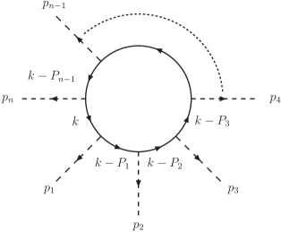
Figure 1: Momentum assignment for the one-loop $n$-point function.

The external momenta $p_{1},\ldots,p_{n}$ (corresponding to the $\sigma$-field) are all flowing out of the diagram and hence sum up to zero. All internal lines are assumed to correspond to scalar propagators with equal masses, the $ith$ one being

$$G_{i}(k)\equiv\frac{1}{(k-P_{i})^{2}-m^{2}}\;,$$ (9)

where we have suppressed the (causal) pole prescription. The loop momentum to be integrated is $k$ and

$$P_{0}\equiv 0\;,\quad P_{i}\equiv p_{1}+\ldots+p_{i}\;,\quad i=1,\ldots,n-1\;.$$ (10)

In terms of the propagators (9) the graph of Fig. 1 represents the momentum integral

$$I_{n,d}\equiv\int\frac{d^{d}k}{(2\pi)^{d}}\prod_{i=0}^{n-1}\frac{1}{(k-P_{i})^{2}-m^{2}}\;.$$ (11)

The denominators appearing in the integrand may be combined by introducing the usual Feynman parameters $x_{0},\ldots\ x_{n-1}$ (with $x_{0}=1-\sum x_{i}$, see App. A) leading to the compact expression

$$I_{n,d}=\int_{0}^{1}[d^{n-1}x]\int\frac{d^{d}\ell_{n}}{(2\pi)^{d}}\frac{\Gamma(n)}{(\ell_{n}^{2}-\Delta_{n})^{n}}\;,$$ (12)

which will henceforth be referred to as the Feynman representation. In (12) we have defined a measure on the $(n-1)$-simplex,

$$[d^{n-1}x]\equiv d^{n}x\;\delta(1-x_{0}-\sum_{i}x_{i})\;,$$ (13)

a shifted 4-momentum

$$\ell_{n}(\mbox{\boldmath$x$})\equiv k-\sum_{i}x_{i}P_{i}\;,$$ (14)

and an effective mass term

$$\Delta_{n}(\mbox{\boldmath$x$})\equiv m^{2}-\sum_{i}x_{i}\bar{x}_{i}P_{i}^{2}+2\sum_{j<i}x_{i}x_{j}P_{i}\cdot P_{j}\;,$$ (15)

employing the abbreviations $\mbox{\boldmath$x$}\equiv(x_{1},\ldots x_{n-1})$, $d^{n}x\equiv dx_{0}\ldots dx_{n-1}$, $\bar{x}_{i}\equiv 1-x_{i}$, and all unconstrained summations extending from $i=1$ to $n-1$. Note that $\Delta_{n}$ is a quadratic form in the $x_{i}$ which may be written in condensed notation Ferroglia et al. (2003),

$$\Delta_{n}(\mbox{\boldmath$x$})=(\mbox{\boldmath$x$},H\mbox{\boldmath$x$})+2(K,\mbox{\boldmath$x$})+L\;,$$ (16)

with the coefficients encoded in the Lorentz invariants

$$H_{ij}\equiv-P_{i}\cdot P_{j}\;,\quad K_{i}\equiv P_{i}^{2}\;,\quad L\equiv m^{2}\;.$$ (17)

The momentum integral in (12) can be found in standard texts (see e.g. Peskin and Schroeder (1995)),

$$\int d^{d}\ell_{n}\,\frac{1}{(\ell_{n}^{2}-\Delta_{n})^{n}}=i(-1)^{n}\frac{\Gamma(n-d/2)}{\Gamma(n)}\frac{\pi^{d/2}}{\Delta_{n}^{n-d/2}}\;,$$ (18)

whereupon (12) becomes

$$I_{n,d}=i\frac{(-1)^{n}}{(4\pi)^{d/2}}\Gamma(n-d/2)\int_{0}^{1}\frac{[d^{n-1}x]}{\Delta_{n}^{n-d/2}(\mbox{\boldmath$x$})}\;.$$ (19)

The hard part still to be done is to integrate over the $n-1$ independent Feynman parameters with the integrand being a complicated rational function of the $x_{i}$. There is no general formula available and, for standard applications, not really required as one is usually only interested in the behaviour of the integrals for small deviation $\epsilon$ from four dimensions, $d=4-2\epsilon$. In App. B we point out the possibility to evaluate the parameter integrals as statistical averages.

Our next goal is to interpret the $x_{i}$ in terms of light-front momentum fractions in the spirit of Weinberg Weinberg (1966) rather than to perform the Feynman parameter integrals. The crucial observation is that the momentum integral (12) may be evaluated in terms of light-front coordinates making use of the generalised Yan formula (8). To this end we rewrite (12) using $d^{d}\ell=(1/2)\,d^{d-2}\ell_{\perp}\,d\ell^{\scriptscriptstyle+}d\ell^{\scriptscriptstyle-}$,

$$I_{n,d}=\int\limits_{0}^{1}[d^{n-1}x]\int\frac{d^{d-2}\ell_{\perp}}{(2\pi)^{d-2}}\frac{d\ell^{\scriptscriptstyle+}d\ell^{\scriptscriptstyle-}}{8\pi^{2}}\frac{\Gamma(n)}{(\ell^{\scriptscriptstyle+}\ell^{\scriptscriptstyle-}-M_{n}^{2})^{n}}\;,$$ (20)

where we have omitted the subscripts $n$ of the integration variables and introduced the effective ‘transverse mass’

$$M_{n}^{2}(\ell_{\perp},x)\equiv\ell_{n,\perp}^{2}+\Delta_{n}(\mbox{\boldmath$x$})\;.$$ (21)

The $\ell^{\scriptscriptstyle-}$-integral is now directly amenable to the generalised Yan formula, the subsequent $\ell^{\scriptscriptstyle+}$-integration over $\delta(\ell^{\scriptscriptstyle+})$ being trivial. We therefore end up with the integral representation

$$I_{n,d}=i\frac{(-1)^{n}}{4\pi}\int\limits_{0}^{1}[d^{n-1}x]\,\int\frac{d^{d-2}\ell_{\perp}}{(2\pi)^{d-2}}\frac{\Gamma(n-1)}{(M_{n}^{2})^{n-1}}\;.$$ (22)

The following remarks are in order. The final integral (22) consists of $n-1$ integrations over Feynman parameters which are the same as in the covariant expression (12) and a Euclidean integral over transverse momenta in dimension $d-2$. This is the structure already discovered by Weinberg for $d=4$ and $n=2$ Weinberg (1966). It therefore seems appropriate to refer to the integral (22) as being in the ‘Weinberg representation’. Its most important property presumably is its manifest Lorentz invariance as the sole dependence of $\Delta_{n}$ on external momenta is in terms of the invariants $P_{i}^{2}$ and $P_{i}\cdot P_{j}$, cf. (15).

Note furthermore that, throughout the derivation leading from (12) to (22), every expression was finite by virtue of dimensional regularisation (dimReg). This is true in particular for the final expression (22) where the original regularisation has resulted in transverse dimReg, originally suggested by Casher Casher (1976). (In this paper we do not discuss infrared singularities which, for $m=0$, show up as endpoint singularities as $x\to 0$ or 1.) Finally, it is easy to see using (18) that performing the transverse momentum integration in (22) exactly reproduces (19).

The next task is to relate the Weinberg representation (22) to the ‘light-front representation’, i.e. the standard integrals encountered in light-front perturbation theory with energy denominators as given in (5). This is the topic of the next sections.

III 2-point function

It seems wise to begin with the simplest case, the scalar 2-point function, i.e. $n=2$ (see Fig. 2). In agreement with standard conventions we set $p_{1}=-p_{2}\equiv p$, $x_{1}\equiv x=1-x_{2}$ and obtain for (14) and (15),

$$\ell_{2} = k-xp\;,$$ (23)

$$\Delta_{2} = m^{2}-x\bar{x}\,p^{2}\;.$$ (24)

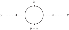
Figure 2: Momentum assignment for the one-loop $2$-point function.

We thus consider the integral

$$I_{2,d}=\int_{0}^{1}dx\,\int\frac{d^{d}\ell_{2}}{(2\pi)^{d}}\frac{1}{(\ell_{2}^{2}-\Delta_{2})^{2}}$$ (25)

and in particular its Weinberg representation,

$$I_{2,d}=\frac{i}{4\pi}\int_{0}^{1}dx\,\int\frac{d^{d-2}\ell_{\perp}}{(2\pi)^{d-2}}\frac{1}{M_{2}^{2}}\;,$$ (26)

with $M_{2}^{2}$ explicitly given by

$$M_{2}^{2}(x,p)=(k_{\perp}-xp_{\perp})^{2}+m^{2}-x\bar{x}p^{2}\;,$$ (27)

according to (21), (23) and (24).

Yan’s formula (7) tells us that the $\ell_{2}^{\scriptscriptstyle+}$-integration leading from (25) to (26) is localised at $\ell_{2}^{\scriptscriptstyle+}=0$ which according to (23) implies

$$x=k^{\scriptscriptstyle+}/p^{\scriptscriptstyle+}\;,\quad dx=dk^{\scriptscriptstyle+}/p^{\scriptscriptstyle+}\;,$$ (28)

identifying $x$ straightforwardly as a longitudinal momentum fraction. We can thus trade the single $x$-integration in (26) for a $k^{\scriptscriptstyle+}$-integration ranging from 0 to $p^{\scriptscriptstyle+}$. To exhibit the light-front energy denominators we have derived the algebraic identity

$$M_{2}^{2}=-\frac{k^{\scriptscriptstyle+}(p^{\scriptscriptstyle+}-k^{\scriptscriptstyle+})}{p^{\scriptscriptstyle+}}\Big{\{}p^{\scriptscriptstyle-}-[k^{\scriptscriptstyle-}]-[p^{\scriptscriptstyle-}-k^{\scriptscriptstyle-}]\Big{\}}\;,$$ (29)

which is proven by simply working out the right-hand side and comparing with (27). It turns out to be useful to abbreviate light-front denominators by means of a bra-ket notation,

$$\langle k_{1},\ldots,k_{n}\,|\,p\rangle\equiv\frac{(p^{\scriptscriptstyle+})^{n-1}}{k_{1}^{\scriptscriptstyle+}\ldots k_{n}^{\scriptscriptstyle+}\,\Big{\{}p^{\scriptscriptstyle-}-[k_{1}^{\scriptscriptstyle-}]-\ldots-[k_{n}^{\scriptscriptstyle-}]\Big{\}}}\;.$$ (30)

Here $p$ denotes the total momentum which is distributed among the $n$ intermediate states labelled by their on-shell momenta $k_{1},\ldots,k_{n}$. The quantity (30) has dimensions of inverse mass squared. It may be interpreted as the perturbative light-front amplitude for a particle with incoming (off-shell) momentum $p$ to consist of $n$ constituents of momenta $k_{i}$ (see Fig. 3) and hence represents an off-shell extension of an $n$-particle light-front wave function.

For scalar fields in $d>2$ the number $n$ will in general not exceed 4 as there are no high-order renormalisable vertices. The situation, however, is different for super-renormalisable theories in $d=2$, e.g. for the sine-Gordon model Griffin (1992); Burkardt (1993).

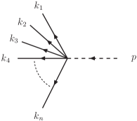
Figure 3: $n$-particle light-front amplitude corresponding to an $n$th order scalar vertex.

Using (30) the propagator (5) can be written as a ‘single-particle’ amplitude,

$$\frac{1}{p^{2}-m^{2}+i\epsilon}=\frac{1}{p^{\scriptscriptstyle+}}\frac{1}{p^{\scriptscriptstyle-}-[p^{\scriptscriptstyle-}]}\equiv\langle p\,|\,p\rangle\;,$$ (31)

and the two-particle amplitude is the inverse of the transverse mass (29)

$$\langle k,p-k\,|\,p\rangle\equiv-1/M_{2}^{2}\;.$$ (32)

Plugging (32) and (28) into (26) finally yields the desired light-front representation,

$$I_{2,d}=-i\int_{0}^{p^{\scriptscriptstyle+}}\frac{dk^{\scriptscriptstyle+}}{4\pi p^{\scriptscriptstyle+}}\int\frac{d^{d-2}k_{\perp}}{(2\pi)^{d-2}}\langle k,p-k\,|\,p\rangle\;.$$ (33)

It is worth reemphasising that this is strictly identical to the covariant expression (25) and the Weinberg representation (26). Using the general result (19) the 2-point function becomes

$$I_{2,d}=i\,\frac{\Gamma(2-d/2)}{(4\pi)^{d/2}}\int_{0}^{1}\frac{dx}{(m^{2}-x\bar{x}\,p^{2})^{2-d/2}}\;,$$ (34)

which makes its Lorentz invariance manifest. Weinberg in Weinberg (1966) has basically obtained (26) in $d=4$ and subsequently shown that the derivatives of (26) and (34) with respect to $p^{2}$ (which are finite in $d=4$) coincide. He did not relate these integrals to the standard light-front representation (33) which was still awaiting its discovery at that time Chang and Ma (1969).

The approach presented in this section suggests an interesting route to evaluating one-loop diagrams in light-front perturbation theory. If one manages to rewrite any light-front representation with all its energy denominators as a Weinberg representation using transverse dimReg one has achieved an elegant way of both doing the transverse integrations and proving Lorentz invariance. All UV divergences should be regularised and one has only to deal with the same IR divergences as are present in the covariant diagram.

IV 3-point function

According to our general formula (12) the scalar 3-point function has the covariant Feynman representation

$$I_{3,d}=\int_{0}^{1}dz\int_{0}^{1-z}dz^{\prime}\,\int\frac{d^{d}\ell_{3}}{(2\pi)^{d}}\frac{2}{(\ell_{3}^{2}-\Delta_{3})^{3}}\;.$$ (35)

The Feynman parameters have been renamed as $z$ and $z^{\prime}$ while $\ell_{3}$ and $\Delta_{3}$ follow from (14) and (15). The latter will be stated explicitly below once we have chosen particular kinematics. Yan’s formula implies the Weinberg representation

$$I_{3,d}=-\frac{i}{4\pi}\int\limits_{0}^{1}[d^{2}z]\int\frac{d^{d-2}\ell_{\perp}}{(2\pi)^{d-2}}\frac{1}{[M_{3}^{2}(\mbox{\boldmath$z$},\ell_{\perp})]^{2}}\;,$$ (36)

with $M_{3}^{2}$ as defined in (21). It is not entirely straightforward to transform (36) into its the light-front representation. One would have to decompose $M_{3}^{2}$ into a sum of energy denominators describing the intermediate 2-particle states. We found it actually simpler to reverse the order of Section III and work ‘backwards’ from the light-front to the Weinberg representation. Still, for the most general 3-point function the associated light-front representation becomes quite tedious to determine. To see what is involved let us rewrite the covariant Feynman diagram using the denominator replacement (31) which yields

$$I_{3,d}=\int\frac{d^{d-2}k_{\perp}}{(2\pi)^{d-2}}\int\frac{dk^{\scriptscriptstyle+}dk^{\scriptscriptstyle-}}{8\pi^{2}}\prod_{i=0}^{2}\langle k+P_{i}\,|\,k+P_{i}\rangle\;.$$ (37)

In order to perform the $k^{\scriptscriptstyle-}$-integration using residue techniques one has to determine the location of the poles in the complex $k^{\scriptscriptstyle-}$-plane. Reinstating the $i\epsilon$ prescriptions the sign of the poles’ imaginary part is given by ${\mbox{sgn}}(k^{\scriptscriptstyle+}+P_{i}^{\scriptscriptstyle+})$. One thus has to consider all orderings of the longitudinal momenta $-P_{i}^{\scriptscriptstyle+}$ and check whether closing a contour yields a contribution Bakker (2000). This is the case if the real $k^{\scriptscriptstyle-}$-axis is pinched between poles. Closer examination reveals that pinching can only happen if the following ‘pinching condition’ is satisfied,

$$\min_{i}(-P_{i}^{\scriptscriptstyle+})<k^{\scriptscriptstyle+}<\max_{i}(-P_{i}^{\scriptscriptstyle+})\;.$$ (38)

Otherwise, all poles will be located either above or below the real axis and the $k^{\scriptscriptstyle-}$-integration yields zero. We thus conclude that the integration region for $k^{\scriptscriptstyle+}$ will be finite with the boundaries given by (38). This confirms and generalises the original findings of Chang and Ma (1969). Shifting the integration variable $k^{\scriptscriptstyle+}$ appropriately one can always achieve a standard integration range for longitudinal momentum from zero up to some maximum value (see examples below).

For the 3-point functions one a priori has $3!=6$ $P_{i}^{\scriptscriptstyle+}$-orderings. Choose one of these and let $k^{\scriptscriptstyle+}$ gradually increase from negative towards positive infinity. To the left of the region (38) one gets zero as all poles are on the same side of the real axis. Pole after pole will cross the axis whenever $k^{\scriptscriptstyle+}=-P_{i}^{\scriptscriptstyle+}$. The final crossing will again result in all poles being to one side and hence a vanishing contribution. For $n=3$ we start with the three poles, say, above the real axis and none below, a configuration which we denote by $(3|0)$. Increasing $k^{\scriptscriptstyle+}$ we successively obtain configurations $(2|1)$, $(1|2)$ and $(0|3)$. Only those with nonzero entries contribute, i.e. $(2|1)$ and $(1|2)$. Thus, for a general $n$-point we expect $n-1$ non-vanishing pole configurations such that the total number of light-front integrals contributing should be

$$N_{n}=(n-1)\,n!\;.$$ (39)

Obviously, the number of integrals grows somewhat stronger than factorially. For the two-point function of the previous section, there are a priori two contributions stemming from the ‘pinching intervals’ $0<k^{\scriptscriptstyle+}<p^{\scriptscriptstyle+}$ and $p^{\scriptscriptstyle+}<k^{\scriptscriptstyle+}<0$. However, both give rise to the same light-front integral representation, as both regions imply $0<x<1$. That’s why in the end there is only one integral left.

For $n=3$ the counting rule (39) implies a total of 12 contributions. Again, depending on the symmetries and kinematics involved, some of those may still vanish. To simplify things we will exploit this fact by considering the popular choice of form factor kinematics. This has been studied extensively in recent years leading to a vast amount of literature. It is impossible to give a complete account of the latter and we only refer the reader to a representative list of references Brodsky et al. (1973); Bakker et al. (2001, 2005); Frankfurt and Strikman (1979); Frederico and Miller (1992); Melikhov and Simula (2002) where the relation between the covariant triangle diagram and light-front perturbation theory has been investigated.

Form factor kinematics amounts to setting

$$p_{1}=-p\;,\quad p_{2}=p^{\prime}\;,\quad p_{3}=-q\;,$$ (40)

and replacing $k\to k-p$. $q$ is interpreted as the probe momentum transfer (Fig. 4). Strictly speaking, for a form factor $p$ and $p^{\prime}$ are on-shell which we do not assume for the time being.

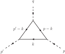
Figure 4: Momentum assignment for the one-loop $3$-point function (form factor kinematics).

The $n=3$ abbreviations then read explicitly

$$M_{3}^{2} = \ell_{3,\perp}^{2}+\Delta_{3}\;,$$ (41)

$$\ell_{3} = k-zp-z^{\prime}p^{\prime}\;,$$ (42)

$$\Delta_{3} = m^{2}-z\bar{z}p^{2}-z^{\prime}\bar{z}^{\prime}p^{\prime 2}+2zz^{\prime}p\cdot p^{\prime}\;.$$ (43)

In what follows we will further assume that the momentum transfer $q$ has $q^{\scriptscriptstyle+}\geq 0$ which includes the simplest case, namely the Drell-Yan-West frame, $q^{\scriptscriptstyle+}=0$. This implies the longitudinal momentum ordering

$$0<p^{\scriptscriptstyle+}\leq p^{\prime{\scriptscriptstyle+}}=p^{\scriptscriptstyle+}+q^{\scriptscriptstyle+}\;,$$ (44)

which in turn determines the location of the $k^{\scriptscriptstyle-}$-poles. Choosing this particular ordering reduces the number of light-front integrals from 12 to 2, which, after residue integration in (37) become

$$I_{3,d} = \frac{-i}{4\pi}\int\frac{d^{d-2}k_{\perp}}{(2\pi)^{d-2}}\int\limits_{0}^{p^{\scriptscriptstyle+}}\frac{dk^{\scriptscriptstyle+}k^{\scriptscriptstyle+}}{p^{\scriptscriptstyle+}p^{\prime{\scriptscriptstyle+}}}\langle p^{\prime}\,|\,k,p^{\prime}-k\rangle\langle k,p-k\,|\,p\rangle$$ (45)

$$- \frac{i}{4\pi}\int\frac{d^{d-2}k_{\perp}}{(2\pi)^{d-2}}\int\limits_{0}^{q^{\scriptscriptstyle+}}\frac{dk^{\scriptscriptstyle+}k^{\scriptscriptstyle+}}{q^{\scriptscriptstyle+}p^{\prime{\scriptscriptstyle+}}}\langle p^{\prime}\,|\,k,p^{\prime}-k\rangle\langle k,q-k\,|\,q\rangle$$

$$\equiv I_{3,d}^{(\mathrm{v})}+I_{3,d}^{(\mathrm{nv})}\;.$$

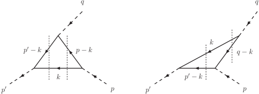
Figure 5: The two contributions to the one-loop $3$-point function (form factor kinematics) in light-front perturbation theory. Dashed vertical lines indicate two-particle denominators. Left: valence contribution; right: nonvalence contribution

Note the $k^{\scriptscriptstyle+}$-measures which will become important in a moment. The second integral in (45) is obtained from the first upon replacing $p\leftrightarrow q$ (which leaves $p^{\prime}=p+q$ invariant). In Fig. 5 we have depicted the associated diagrams usually referred to as the ‘valence’ and ‘nonvalence contribution’, hence the superscripts in (45). The light-front time direction is pointing from right to left. Hence, in the second diagram the first vertex (labelled by $q$) corresponds to pair creation so that the $p$-vertex corresponding to the incoming particle cannot be interpreted as a light-front wave function with $p$ being on shell Sawicki (1992).

The question now is how to obtain the Weinberg representation (36) from the light-front one given by (45). The answer is technically somewhat tricky. One first generalises (28) to $n=3$ by defining the longitudinal momentum fractions

$$x\equiv k^{\scriptscriptstyle+}/p^{\scriptscriptstyle+}\;,\quad x^{\prime}\equiv k^{\scriptscriptstyle+}/p^{\prime{\scriptscriptstyle+}}\;.$$ (46)

Naturally one is tempted to follow the case $n=2$ and identify $x$ and $x^{\prime}$ directly with $z$ and $z^{\prime}$ from (36). Unfortunately, this does not make sense as the former are not independent,

$$x^{\prime}=\frac{p^{\scriptscriptstyle+}}{p^{\prime{\scriptscriptstyle+}}}x\equiv\kappa x\;.$$ (47)

However, we may follow the treatment of the 2-point function in rewriting the light-front denominators in (45) by means of (32). This yields the fairly compact expression

$$I_{3,d}^{\mathrm{(v)}}=-\kappa\frac{i}{4\pi}\int\frac{d^{d-2}k_{\perp}}{(2\pi)^{d-2}}\int\limits_{0}^{1}\frac{dx\,x}{M_{2}^{2}M_{2}^{\prime 2}}\;,$$ (48)

with $M_{2}^{2}$ as given in (27) and $M_{2}^{\prime 2}\equiv M_{2}^{2}(x^{\prime},p^{\prime})$. Note the appearance of the factor $\kappa=p^{\scriptscriptstyle+}/p^{\prime{\scriptscriptstyle+}}$ in front of the integral. We still have only one Feynman parameter $x$ in (48), but this is easily remedied by combining the two denominators with a second parameter $y$,

$$I_{3,d}^{\mathrm{(v)}}=-\frac{i\kappa}{4\pi}\int\frac{d^{d-2}k_{\perp}}{(2\pi)^{d-2}}\int\limits_{0}^{1}dxx\int\limits_{0}^{1}dy\frac{1}{\Big{[}yM_{2}^{2}+\bar{y}M_{2}^{\prime 2}\Big{]}^{2}}\;.$$ (49)

This starts to look promising and indeed the ‘miracle’ happens. A lengthy but straightforward calculation shows the identity

$$y\,M_{2}^{2}(x,p)+\bar{y}M_{2}^{2}(x^{\prime},p^{\prime})=M_{3}^{2}(z,z^{\prime},\ell_{3,\perp})\;,$$ (50)

if the following identifications are made,

$$z\equiv xy\;,\quad z^{\prime}\equiv x\bar{y}\;$$ (51)

and $\ell_{3}$ from (42) is used. Working out the Jacobian yields the additional relation

$$dz\,dz^{\prime}=x\,dx\,dy\;.$$ (52)

This is exactly the measure appearing in expression (49) which thus turns into the Weinberg representation

$$I_{3,d}^{\mathrm{(v)}}=-\frac{i\kappa}{4\pi}\int\limits_{0}^{1}dz\int\limits_{0}^{1-z}dz^{\prime}\int\frac{d^{d-2}\ell_{\perp}}{(2\pi)^{d-2}}\frac{1}{[M_{3}^{2}(z,z^{\prime},\ell_{\perp})]^{2}}\;.$$ (53)

For the nonvalence contribution of (45) we simply replace $p$ by $q$ wherever the former appears. This leads to the same integrals as in (53) the only difference being the prefactor replacement $\kappa\to 1-\kappa$. Adding both contributions we finally end up with

$$I_{3,d}=-\frac{i}{4\pi}\int\limits_{0}^{1}dz\int\limits_{0}^{1-z}dz^{\prime}\int\frac{d^{d-2}\ell_{\perp}}{(2\pi)^{d-2}}\frac{1}{[M_{3}^{2}(z,z^{\prime},\ell_{\perp})]^{2}}\;.$$ (54)

Note that $\kappa$ is invariant under longitudinal boosts under which $p^{\scriptscriptstyle+}\to\lambda p^{\scriptscriptstyle+}$. Hence, both contributions, $I_{3,d}^{\mathrm{(v)}}$ and $I_{3,d}^{\mathrm{(nv)}}$ are separately boost invariant. Complete Lorentz invariance, however, is only achieved by adding both terms so that the $\kappa$ dependence cancels.

V Discussion and conclusion

Let us summarise our findings. We have represented the Feynman diagram $I_{n,d}$ for a general scalar $n$-point function in basically three different ways all of which are strictly finite by means of dimReg. The different representations are:

1. Feynman representation

$$I_{n,d}=\int_{0}^{1}[d^{n-1}x]\int\frac{d^{d}\ell}{(2\pi)^{d}}\frac{\Gamma(n)}{(\ell^{2}-\Delta_{n})^{n}}\;.$$ (55)

This is the standard textbook representation obtained after combining denominators with Feynman parameters. The momentum integral is straightforwardly done with formula (18).

2. Weinberg representation

$$I_{n,d}=i\frac{(-1)^{n}}{4\pi}\int\limits_{0}^{1}[d^{n-1}x]\,\int\frac{d^{d-2}\ell_{\perp}}{(2\pi)^{d-2}}\frac{\Gamma(n-1)}{(\ell_{\perp}^{2}+\Delta_{n})^{n-1}}\;.$$ (56)

This representation is obtained from (55) by performing the $\ell^{\scriptscriptstyle-}$-integration using Yan’s formula (8). Afterwards the integral is localised at vanishing longitudinal momentum, $\ell^{\scriptscriptstyle+}=0$, by means of a delta function which is trivially integrated in turn. Note that (56) is manifestly invariant as $\Delta_{n}$ only depends on Lorentz scalars. Again, the momentum integration may be done with (18). A precursor of (56) has already been obtained by Weinberg Weinberg (1966).

3. Light-front representation

For the two- and three-point functions ($n=2$ and 3, respectively) we have succeeded in explicitly relating the Weinberg representation (56) to its light-front analogue. That this can be done, in particular for the nontrivial case $n=3$, is one of the main results of this paper. Explicitly, one has for $n=2$,

$$I_{2,d}=-i\int_{0}^{p^{\scriptscriptstyle+}}\frac{dk^{\scriptscriptstyle+}}{4\pi p^{\scriptscriptstyle+}}\int\frac{d^{d-2}k_{\perp}}{(2\pi)^{d-2}}\langle k,p-k\,|\,p\rangle\;.$$ (57)

and for $n=3$,

$$I_{3,d} = \frac{-i}{4\pi}\int\frac{d^{d-2}k_{\perp}}{(2\pi)^{d-2}}\int\limits_{0}^{p^{\scriptscriptstyle+}}\frac{dk^{\scriptscriptstyle+}k^{\scriptscriptstyle+}}{p^{\scriptscriptstyle+}p^{\prime{\scriptscriptstyle+}}}\langle p^{\prime}\,|\,k,p^{\prime}-k\rangle\langle k,p-k\,|\,p\rangle$$ (58)

$$+ (p\leftrightarrow q)\;.$$

The technical challenge is to transform Feynman parameters into longitudinal momentum fractions (which is straightforward only for $n=2$) and to factorise the covariant denominator in (56) in terms of light-front energy denominators, abbreviated via the bracket notation $\langle k_{1},\ldots k_{n}|p\rangle$ from (30).

Obviously, one would like to have a general result for the light-front representation of $I_{n,d}$ for arbitrary $n$. While this might be rather involved, it seems reasonable to expect at least a recursion type formula relating the denominator expressions $M_{n}^{2}$ to $M_{n-1}^{2}$, cf. (50), as well as relations between integration parameters analogous to (51). Clearly, this deserves further investigation.

As a by-product of this investigation we obtain alternative ways of regularising perturbative light-front wave functions. The latter can be read off by writing the form factor integrand of $I_{3,d}$ (for zero momentum transfer) as a wave function squared and putting external momenta on-shell, $p^{2}=p^{\prime 2}=M^{2}$. This yields wave functions Terent’ev (1976); Frankfurt and Strikman (1979)

$$\psi(x,\mbox{\boldmath$\ell$}_{\perp})=\frac{N}{M^{2}-(\mbox{\boldmath$\ell$}_{\perp}^{2}+m^{2})/x\bar{x}}\;,$$ (59)

where $N$ is a ‘normalisation’ constant. The use of inverted commas serves to remind us of the fact that normalisation requires regularisation, and dimReg indeed does the job for us. At zero transverse separation (which defines the distribution amplitude), for instance, we find

$$\int d^{2}\ell_{\perp}\,\psi(x,\mbox{\boldmath$\ell$}_{\perp})\sim x\bar{x}\,\frac{1}{\epsilon}+\mbox{finite terms}\;,$$ (60)

with $\epsilon=2-d/2$ as usual. The same result is obtained within analytic regularisation, where the denominator in (59) is raised to power $\nu$ and $\epsilon=\nu-1$.

With hindsight it is the Weinberg representation (56) which looks most appealing from a ‘noncovariant’ point of view. Thus, the intriguing question arises as to whether it is possible to derive this representation directly from a modified light-front Lagrangian or Hamiltonian. At present, we do not have a satisfactory answer but it definitely seems worthwhile to keep looking for it.

Appendix A Feynman parameters

There are several equivalent ways of representing products of denominators in terms of Feynman parameters. (The reference to Feynman is actually misleading, as it was Schwinger who originally suggested the method. This was explicitly stated by Feynman himself in Feynman (1949) and was recently emphasized in Milton (2006).)

The most straightforward formula presumably is the following,

$$\frac{1}{a_{0}a_{1}\ldots a_{n-1}}=\int d^{n}x\,\frac{\Gamma(n)\,\delta(1-\sum_{i=0}^{n-1}x_{i})}{(a_{0}x_{0}+\ldots+a_{n-1}x_{n-1})^{n}}\;,$$ (61)

with the (flat) measure $d^{n}x\equiv dx_{0}dx_{1}\ldots dx_{n-1}$. The delta function entails that the integration actually extends over the $(n-1)$-simplex with measure $[d^{n-1}x]$. Depending on the variables (Feynman parameters) chosen, this measure takes on many different forms, each with its own integration boundaries. While proving the validity of the different representations by induction is straightforward, it is a nontrivial task to find the variable transformations relating them.

The following representation (see e.g. Ho-Kim and Pham (1998)) was particularly useful for our purposes,

$$\frac{1}{a_{0}a_{1}\ldots a_{n-1}}=\int\limits_{0}^{1}dx_{1}\int\limits_{0}^{1-x_{1}}dx_{2}\ldots\int\limits_{0}^{1-x_{1}-\ldots-x_{n-2}}dx_{n-1}\frac{\Gamma(n)}{\Big{[}a_{0}(1-x_{1}-\ldots-x_{n-2})+a_{1}x_{1}+\ldots+a_{n-1}x_{n-1}\Big{]}^{n}}\;.$$ (62)

A different but equivalent way of writing this is (see e.g. Jauch and Rohrlich (1955), App. A5 or Quigg (1983), App. B.3)

$$\frac{1}{a_{0}a_{1}\ldots a_{n-1}}=\int\limits_{0}^{1}du_{1}u_{1}^{n-2}\int\limits_{0}^{1}du_{2}u_{2}^{n-3}\ldots\int\limits_{0}^{1}du_{n-1}\frac{\Gamma(n)}{\Big{[}(a_{0}-a_{1})u_{1}\ldots u_{n-1}+(a_{1}-a_{2})u_{1}\ldots u_{n-2}+\ldots+a_{n-1}\Big{]}^{n}}\;.$$ (63)

Appendix B Tensor integrals and the Dirichlet distribution

Within the Passarino-Veltman scheme there is a standard procedure to reduce tensor integrals (which typically appear for nonzero spin) to scalar integrals, see e.g. Weinzierl (2003). The main differences to the integrals encountered so far in this paper are a shift in dimension, $d\to d^{\prime}$, and nontrivial exponents in the denominators,

$$(k-P_{i})^{2}-m^{2}\to[(k-P_{i})^{2}-m^{2}]^{\nu_{i}}\;.$$ (64)

Effectively, this changes the scalar integrals (11) according to

$$I_{n,d}\to I_{n^{\prime},d^{\prime},\mbox{\scriptsize\boldmath$\nu$}}\;,$$ (65)

where $\nu$ is the vector formed from the exponents $\nu_{i}$ in (64). Explicitly, we have instead of (11)

$$I_{n,d,\mbox{\scriptsize\boldmath$\nu$}}=\int\frac{d^{d}k}{(2\pi)^{d}}\prod_{i=0}^{n-1}\frac{1}{[(k-P_{i})^{2}-m^{2}]^{\nu_{i}}}\;,$$ (66)

where we omitted the primes on $n$ and $d$ for simplicity. Again, upon keeping $d$ fixed and setting $\nu_{i}=1+\epsilon$ this integral may alternatively be viewed as the analytic regularisation of $I_{n,d}$. We will not go down this road, however, but rather stick with the dimReg interpretation.

Introducing Feynman parameters as before (66) becomes

$$I_{n,d,\mbox{\scriptsize\boldmath$\nu$}}=\int\limits_{0}^{1}\frac{[d^{n-1}x]}{B(\mbox{\boldmath$\nu$})}\prod_{i=0}^{n-1}x_{i}^{\nu_{i}-1}\int\frac{d^{d}\ell_{n}}{(2\pi)^{d}}\frac{1}{(\ell_{n}^{2}-\Delta_{n})^{|\nu|}}\;,$$ (67)

where $|\nu|\equiv\nu_{0}+\nu_{1}+\ldots+\nu_{n-1}$ and $B$ denotes the multinomial Beta function,

$$B(\mbox{\boldmath$\nu$})\equiv\frac{\Gamma(\nu_{0})\ldots\Gamma(\nu_{n-1})}{\Gamma(|\nu|)}\;.$$ (68)

Somewhat surprisingly, the integrals (67) have a nice statistical interpretation. If one introduces the Dirichlet distribution Devroye (1986); O’Hagan and Forster (2004) on the $(n-1)$-simplex, which corresponds to a probability density

$$\rho_{\mathrm{Dir}}(\mbox{\boldmath$x$},\mbox{\boldmath$\nu$})\equiv\frac{1}{B(\mbox{\boldmath$\nu$})}\prod_{i=0}^{n-1}x_{i}^{\nu_{i}-1}\,\delta\left(1-\sum_{i=0}^{n-1}x_{i}\right)\;,$$ (69)

one may define the expectation values

$$\left\langle f(\mbox{\boldmath$x$})\right\rangle_{\,\mathrm{Dir}(\mbox{\scriptsize\boldmath$\nu$})}\equiv\int\limits_{0}^{1}dx_{0}\ldots dx_{n-1}\,\rho_{\mathrm{Dir}}(\mbox{\boldmath$x$},\mbox{\boldmath$\nu$})\,f(\mbox{\boldmath$x$})\;.$$ (70)

Hence, the integrals (67) are nothing but the expectation values

$$I_{n,d,\mbox{\scriptsize\boldmath$\nu$}}=\left\langle\int\frac{d^{d}\ell_{n}}{(2\pi)^{d}}\frac{1}{[\ell_{n}^{2}(\mbox{\boldmath$x$})-\Delta_{n}(\mbox{\boldmath$x$})]^{|\nu|}}\right\rangle_{\mathrm{Dir}(\mbox{\scriptsize\boldmath$\nu$})}\;,$$ (71)

with the momentum integral to be evaluated according to (18). We conclude these remarks with the the scalar integral discussed in the main part,

$$I_{n,d}=\left\langle\int\frac{d^{d}\ell_{n}}{(2\pi)^{d}}\frac{1}{[\ell_{n}^{2}(\mbox{\boldmath$x$})-\Delta_{n}(\mbox{\boldmath$x$})]^{n}}\right\rangle_{\mathrm{Dir}(\mbox{\scriptsize\boldmath$1$})}\;.$$ (72)

and note that Dir$(\mbox{\boldmath$1$})$ represents the uniform distribution on the simplex.

Obviously, for a reasonably large number of external legs it should be feasible to evaluate the integrals (71) and (72) by Monte Carlo techniques. Whether this makes sense near the physical number of dimensions, $d\to 4$, remains to be seen. Clearly, one has to deal with the usual UV divergences in this case.

References

- Brown and Feynman (1952) L. M. Brown and R. P. Feynman, Phys. Rev. 85, 231 (1952).
- ’t Hooft and Veltman (1979) G. ’t Hooft and M. J. G. Veltman, Nucl. Phys. B153, 365 (1979).
- Passarino and Veltman (1979) G. Passarino and M. J. G. Veltman, Nucl. Phys. B160, 151 (1979).
- Bardin and Passarino (1999) D. Y. Bardin and G. Passarino, The standard model in the making: Precision study of the electroweak interactions (Clarendon, Oxford, UK, 1999).
- Denner (1993) A. Denner, Fortschr. Phys. 41, 307 (1993).
- Weinberg (1966) S. Weinberg, Phys. Rev. 150, 1313 (1966).
- Chang and Ma (1969) S.-J. Chang and S.-K. Ma, Phys. Rev. 180, 1506 (1969).
- Kogut and Soper (1970) J. B. Kogut and D. E. Soper, Phys. Rev. D1, 2901 (1970).
- Dirac (1949) P. A. M. Dirac, Rev. Mod. Phys. 21, 392 (1949).
- Rohrlich (1971) F. Rohrlich, Acta Physica Austriaca, Suppl. 8, 277 (1971).
- Burkardt (1996) M. Burkardt, Adv. Nucl. Phys. 23, 1 (1996), eprint hep-ph/9505259.
- Brodsky et al. (1998) S. J. Brodsky, H.-C. Pauli, and S. S. Pinsky, Phys. Rept. 301, 299 (1998), eprint hep-ph/9705477.
- Yamawaki (1998) K. Yamawaki (1998), in: QCD, Light-Cone Physics and Hadron Phenomenology, C.-R. Ji, D.-P. Min., eds., World Scientific, Singapore 1998., eprint hep-th/9802037.
- Heinzl (2000) T. Heinzl (2000), Procceedings of the 39th Schladming Winter School, Lecture Notes in Physics 572, Springer, Berlin, 2001, eprint hep-th/0008096.
- Weinberg (1995) S. Weinberg, The quantum theory of fields. Vol. 1: Foundations (Cambridge University Press, Cambridge, UK, 1995).
- Brodsky et al. (1973) S. J. Brodsky, R. Roskies, and R. Suaya, Phys. Rev. D8, 4574 (1973).
- Lepage and Brodsky (1980) G. P. Lepage and S. J. Brodsky, Phys. Rev. D22, 2157 (1980).
- Chang et al. (1973) S.-J. Chang, R. G. Root, and T.-M. Yan, Phys. Rev. D7, 1133 (1973).
- Chang and Yan (1973) S.-J. Chang and T.-M. Yan, Phys. Rev. D7, 1147 (1973).
- Yan (1973a) T.-M. Yan, Phys. Rev. D7, 1760 (1973a).
- Yan (1973b) T.-M. Yan, Phys. Rev. D7, 1780 (1973b).
- Sokolov and Shatnii (1979) S. Sokolov and A. Shatnii, Theor. Math. Phys. 37, 1029 (1979).
- Kvinikhidze and Khvedelidze (1989) A. N. Kvinikhidze and A. M. Khvedelidze, Theor. Math. Phys. 78, 252 (1989).
- Maskawa and Yamawaki (1976) T. Maskawa and K. Yamawaki, Prog. Theor. Phys. 56, 270 (1976).
- Heinzl (2003) T. Heinzl (2003), Proceedings of the international workshop on Light-Cone Physics: Hadrons and Beyond, IPPP/03/71, Durham, 2003; S. Dalley, ed., eprint hep-th/0310165.
- Ritus (1972) V. Ritus, Ann. Phys. 69, 555 (1972).
- Schmidt (1974) M. G. Schmidt, Phys. Rev. D 9, 408 (1974).
- Bakker et al. (2005) B. L. G. Bakker, M. A. DeWitt, C.-R. Ji, and Y. Mishchenko, Phys. Rev. D72, 076005 (2005).
- Bakker et al. (2001) B. L. G. Bakker, H.-M. Choi, and C.-R. Ji, Phys. Rev. D63, 074014 (2001), eprint hep-ph/0008147.
- Bakker and Ji (2000) B. L. G. Bakker and C.-R. Ji, Phys. Rev. D62, 074014 (2000), eprint hep-th/0003105.
- Bakker (2000) B. L. G. Bakker (2000), Procceedings of the 39th Schladming Winter School, Lecture Notes in Physics 572, Springer, Berlin, 2001.
- Burkardt and Langnau (1991) M. Burkardt and A. Langnau, Phys. Rev. D44, 3857 (1991).
- Griffin (1992) P. A. Griffin, Phys. Rev. D46, 3538 (1992), eprint hep-th/9207082.
- Burkardt (1993) M. Burkardt, Phys. Rev. D47, 4628 (1993).
- Heinzl (2002) T. Heinzl (2002), eprint hep-th/0212202.
- Speer (1968) E. Speer, J. Math. Phys. 9, 1404 (1968).
- Mansfield (2006) P. Mansfield, JHEP 03, 037 (2006), eprint hep-th/0511264.
- Ettle and Morris (2006) J. H. Ettle and T. R. Morris, JHEP 08, 003 (2006), eprint hep-th/0605121.
- Ferroglia et al. (2003) A. Ferroglia, M. Passera, G. Passarino, and S. Uccirati, Nucl. Phys. B650, 162 (2003), eprint hep-ph/0209219.
- Peskin and Schroeder (1995) M. Peskin and D. Schroeder, An Introduction to Quantum Field Theory (Addison-Wesley, Reading, Mass., 1995).
- Casher (1976) A. Casher, Phys. Rev. D14, 452 (1976).
- Frankfurt and Strikman (1979) L. L. Frankfurt and M. I. Strikman, Nucl. Phys. B148, 107 (1979).
- Frederico and Miller (1992) T. Frederico and G. A. Miller, Phys. Rev. D45, 4207 (1992).
- Melikhov and Simula (2002) D. Melikhov and S. Simula, Phys. Rev. D65, 094043 (2002), eprint hep-ph/0112044.
- Sawicki (1992) M. Sawicki, Phys. Rev. D46, 474 (1992).
- Terent’ev (1976) M. Terent’ev, Sov. J. Nucl. Phys. 24, 106 (1976).
- Feynman (1949) R. P. Feynman, Phys. Rev. 76, 769 (1949).
- Milton (2006) K. A. Milton (2006), eprint physics/0606153.
- Ho-Kim and Pham (1998) Q. Ho-Kim and X.-Y. Pham, Elementary Particles and their Interactions (Springer, Berlin, Heidelberg, 1998).
- Jauch and Rohrlich (1955) J. Jauch and F. Rohrlich, The Theory of Photons and Electrons (Addison-Wesley, Cambridge, Mass., 1955).
- Quigg (1983) C. Quigg, Gauge Theories of the Strong, Weak and Electromagnetic Interactions, Frontiers in Physics, Vol. 56 (Benjamin/Cummings, Menlo Park, 1983).
- Weinzierl (2003) S. Weinzierl (2003), eprint hep-th/0305260.
- Devroye (1986) L. Devroye, Non-Uniform Random Variate Generation (Springer, 1986), available online at http://cg.scs.carleton.ca/ luc/rnbookindex.html.
- O’Hagan and Forster (2004) A. O’Hagan and J. Forster, Bayesian Inference, vol. 2B of Kendall’s Advanced Theory of Statistics (Arnold, 2004).