Constraints on flavor-dependent long range forces
from solar neutrinos and KamLAND

Abstract

Flavor-dependent long range (LR) leptonic forces, like those mediated by the $L_{e}-L_{\mu}$ or $L_{e}-L_{\tau}$ gauge bosons, constitute a minimal extension of the standard model that preserves its renormalizability. We study the impact of such interactions on the solar neutrino oscillations when the interaction range $R_{LR}$ is much larger than the Earth-Sun distance. The LR potential can dominate over the standard charged current potential inside the Sun in spite of strong constraints on the coupling $\alpha$ of the LR force coming from the atmospheric neutrino data and laboratory search for new forces. We demonstrate that the solar and atmospheric neutrino mass scales do not get trivially decoupled even if $\theta_{13}$ is vanishingly small. In addition, for $\alpha\mathrel{\hbox to0.0pt{\lower 4.0pt\hbox{\hskip 1.0pt$\sim$}\hss}\raise 1.0pt\hbox{$>$}}10^{-52}$ and normal hierarchy, resonant enhancement of $\theta_{13}$ results in nontrivial energy dependent effects on the $\nu_{e}$ survival probability. We perform a complete three generation analysis, and obtain constraints on $\alpha$ through a global fit to the solar neutrino and KamLAND data. We get the $3\sigma$ limits $\alpha_{e\mu}<3.4\times 10^{-53}$ and $\alpha_{e\tau}<2.5\times 10^{-53}$ when $R_{LR}$ is much smaller than our distance from the galactic center. With larger $R_{LR}$, the collective LR potential due to all the electrons in the galaxy becomes significant and the constraints on $\alpha$ become stronger by upto two orders of magnitude.

I Introduction

The standard electroweak model is now a well-established theory but it is believed to be incomplete and one expects some physics beyond the standard model (SM) to exist. Most extensions of SM postulate new physics at scales higher than the electroweak scales starting from TeV to the grand unification or Planck scale. There however exists an interesting possibility that new physics may exist at scales below the electroweak scale. This may arise from the existence of exactly or nearly massless gauge foot or Higgs bosons axion ; singletm ; tripletm which have remained invisible because of their very feeble couplings to the known matter. Various scenarios involving new physics at low energy and their possible signatures hall ; mv ; masso ; mj1 ; mj2 have been studied.

Gauged extension of the SM is one possible scenario with new physics below the electroweak scale. Such a possibility is strongly constrained theoretically from the renormalizability, however there exist foot three possible $U(1)_{X}$ gauge extensions of the standard model which are anomaly free with minimal matter content. These correspond to $X=L_{e}-L_{\mu},~{}L_{e}-L_{\tau},~{}L_{\mu}-L_{\tau}$. The extra gauge boson corresponding to $U(1)_{X}$ may not have been discovered if it is very heavy or if it is (nearly) massless but couples to the matter very weakly. The former possibility is analyzed in foot ; vga . The latter possibility, first suggested in mj1 , is strongly constrained by the search for the long range (LR) forces lr1 ; lr2 .

Unlike the gravitational force, the $U(1)_{X}$ induced force couples only to the electron (and neutrino) density inside a massive object. As a consequence, the resulting acceleration experienced by an object depends on its leptonic content and mass. Such forces that violate the equivalence principle are strongly constrained. In case of the force with a range of $\sim$AU, the most stringent bound comes from lunar ranging lr1 ; lr2 which measures the differential acceleration of the Earth and moon towards the Sun. If $\alpha$ denotes the strength of the long range potential then these experiments imply $\alpha<3.4\times 10^{-49}$ ($2\sigma$) for a range $\lambda\mathrel{\hbox to0.0pt{\lower 4.0pt\hbox{\hskip 1.0pt$\sim$}\hss}\raise 1.0pt\hbox{$>$}}10^{13}$cm.

The flavor-dependent long range force masso induced for example by $L_{e}-L_{\mu,\tau}$ mj1 ; mj2 can still influence neutrino oscillation in spite of such strong constraints on $\alpha$. This happens because (i) the $X$-charge of the electron flavor is opposite to that of muon or tau flavor, so that these twox flavors propagate differently in matter and (ii) the large number of electrons (e.g. inside the Sun) and the long range of interaction compensates for the smallness of coupling and gives rise to a significant potential. For example, the electrons inside the Sun generate a potential $V_{e\beta}$ at the Earth surface given by mj1

$$V_{e\beta}^{\odot}(R_{es})=\alpha_{e\beta}\frac{N_{e}^{\odot}}{R_{es}}\approx 1.3\times 10^{-11}\rm{eV}\left(\frac{\alpha_{e\beta}}{10^{-50}}\right)\;,$$ (1)

where $\alpha_{e\beta}=\frac{g_{e\beta}^{2}}{4\pi}$ corresponds to the gauge coupling of $L_{e}-L_{\beta}~{}(\beta=\mu,\tau)$ symmetry which we will sometimes collectively refer to as $\alpha$. Here $N_{e}^{\odot}\sim 10^{57}$ is the total number of electrons inside the Sun bahcall and $R_{es}$ is the Sun-Earth distance $\approx 7.6\times 10^{26}$ GeV^-1. This is to be compared with the typical value of $\Delta m^{2}/E\sim 10^{-12}$ eV for the atmospheric neutrinos. It follows that $V_{e\beta}$ can induce significant corrections to neutrino oscillations at the Earth even for $\alpha\sim 10^{-50}$.

One can define a parameter

$$\xi\equiv\frac{2EV_{e\beta}}{\Delta m^{2}}$$ (2)

which measures the effect of the long range force in any given neutrino oscillation experiment. The bound on $\alpha$ from lr1 ; lr2 implies that $\xi<750$ in atmospheric or a typical long base line experiment, while $\xi<35$ for the typical parameters of the KamLAND experiment. Relatively large values of $\xi$ tend to suppress the atmospheric neutrino oscillations. The observed oscillations can then be used to put a stronger constraint on $\alpha$ which were analyzed in mj1 . One finds the improved 90% C. L. bound

$$\alpha_{e\mu}<5.5\times 10^{-52}\;,\;\alpha_{e\tau}<6.4\times 10^{-52}$$ (3)

in case of the $L_{e}-L_{\mu,\tau}$ symmetry respectively.

With the improved bound on $\alpha$ given in (3), the value of $\xi$ for KamLAND becomes rather small: $\xi<0.06$. So one expects the KamLAND results to be influenced by the LR interactions to a very small extent. However, the potential $V_{e\beta}$ at the surface of the Sun is $V_{e\beta}^{\odot}(r_{\odot})\approx 2.8\times 10^{-9}(\alpha_{e\beta}/10^{-50})$ eV, which may be compared with the MSW contribution $V_{CC}\approx 6.0\times 10^{-12}$ eV at $r=0.05~{}r_{\odot}$. Therefore one expects the long range potential to change or disturb the MSW LMA solution of the solar neutrino problem lma . Note that the effects on the solar and KamLAND experiments are qualitatively different, since KamLAND only probes the potential at the Earth given in eq. (1) while the solar neutrinos experience a long range potential that varies with the distance from the center of the Sun. It is thus important to do a combined analysis of these two experiments.

The aim of this paper is to discuss new physical effects associated with this force and also make a quantitative analysis of the combined solar and KamLAND data to obtain a bound on $\alpha$. It turns out that the long range potential produces physically interesting and quantitatively significant effects which can be used to constrain its strength. The bound obtained on $\alpha$ is more stringent than that obtained mj1 from the atmospheric results alone by more than an order of magnitude. If $R_{LR}\mathrel{\hbox to0.0pt{\lower 4.0pt\hbox{\hskip 1.0pt$\sim$}\hss}\raise 1.0pt\hbox{$>$}}R_{\rm gal}$ where $R_{\rm gal}$ is our distance from the galactic center $\sim$ 10 kpc, the constraints become even stronger by upto two orders of magnitude.

The plan of the paper is as follows. In Sec. II we present our basic formalism where we describe the main features of the LR potential inside and outside the Sun. In Sec. III, we present an analytic discussion of our results on neutrino masses, mixing angles and the resonances they undergo in case of the $L_{e}-L_{\mu}$ symmetry. The corresponding analysis for the $L_{e}-L_{\tau}$ is similar and the relevant analytic expressions are given in the appendix A. Sec. IV analyzes the KamLAND and the solar neutrino data numerically to obtain bounds on $\alpha$ for $R_{LR}\ll R_{\rm gal}$. The case $R_{LR}\mathrel{\hbox to0.0pt{\lower 4.0pt\hbox{\hskip 1.0pt$\sim$}\hss}\raise 1.0pt\hbox{$>$}}R_{\rm gal}$ is analyzed in Sec. V. A summary of the results is given in Sec. VI. In addition, appendix B gives a brief discussion of the impact of the LR potential on the neutrinos from a core collapse supernova.

II Formalism

We consider the standard electroweak model with its minimal fermionic content but assume the presence of an additional gauged $U(1)_{X}$ symmetry. The cancellation of anomalies requires $X=L_{e}-L_{\mu},L_{e}-L_{\tau}$ or $L_{\mu}-L_{\tau}$ foot . The last symmetry does not play any significant role in the solar neutrino oscillations because of the absence of muons or tau leptons inside the Sun (or Earth). We will therefore concentrate on the first two and the couplings of the mediating vector bosons. The value of $\alpha$ is positive in this case.

The observed neutrino oscillations imply that the $U(1)_{X}$ gauge symmetry cannot be an exact symmetry in nature. This is easy to argue. If it were exact, then the effective five dimensional neutrino mass operator following from any mechanism (e.g. seesaw) would be invariant under it. Consider the case of $L_{e}-L_{\mu}$. Invariance under this dictates the following structure for the effective neutrino mass matrix:

$$m_{eff}=\left(\begin{array}[]{ccc}0&m_{e\mu}&0\\ m_{e\mu}&0&0\\ 0&0&m_{\tau\tau}\end{array}\right)\;.$$ (4)

This structure implies a Dirac and a Majorana neutrino which remain unmixed and therefore cannot give any neutrino oscillations. Thus $L_{e}-L_{\mu}$ needs to be broken. The symmetry breaking scale required to generate the solar scale $\Delta m_{12}^{2}$ would be $\Delta m_{12}^{2}/m_{e\mu}$. With $\Delta m_{12}^{2}\sim 10^{-4}$ eV² corresponding to the solar mass difference and $m_{e\mu}\sim 0.1$ eV corresponding to the degenerate neutrino mass, $\Delta m_{12}^{2}/m_{e\mu}$ is required to be at least $10^{-3}$ eV. A similar conclusion also holds in the case of the unbroken $L_{e}-L_{\tau}$ symmetry.

The size of the $U(1)_{X}$ breaking as required above can be consistent with a nearly massless gauge boson since the corresponding coupling $g$ in this case is required to be very small ($\mathrel{\hbox to0.0pt{\lower 4.0pt\hbox{\hskip 1.0pt$\sim$}\hss}\raise 1.0pt\hbox{$<$}}10^{-24}$) from the search of the long range forces lr1 ; lr2 . The required smallness of the coupling also ensures that the relatively large $U(1)_{X}$ breaking in the neutrino sector is consistent with a very light gauge boson. In fact, a Higgs vacuum expectation value of a few GeV can lead to a gauge boson corresponding to the Earth-Sun range with $g\sim 10^{-26}-10^{-27}$ and can imply a relatively large neutrino splitting mj1 .

The most significant effect of the light gauge bosons would be in the solar neutrino oscillations. The coupling of the solar electrons to the $L_{e}-L_{\mu,\tau}$ gauge bosons would generate a long range potential. If $n_{e}(r)$ denotes the spherically symmetric electron number density inside the Sun then the long range potential is given by

$$V_{e\beta}^{\odot}(r<r_{\odot})=4\pi\alpha_{e\beta}\int_{r}^{\infty}\frac{dr^{\prime}}{r^{\prime 2}}~{}\int_{0}^{r^{\prime}}r^{\prime\prime 2}n_{e}(r^{\prime\prime})dr^{\prime\prime}\;.$$ (5)

Outside the Sun,

$$V_{e\beta}^{\odot}(r>r_{\odot})=\frac{4\pi\alpha_{e\beta}}{r}\int_{0}^{r_{\odot}}r^{\prime\prime 2}n_{e}(r^{\prime\prime})dr^{\prime\prime}=\frac{\alpha_{e\beta}}{r}N_{e}^{\odot}\;.$$ (6)

The approximate profile

$$n_{e}(r)\sim 245~{}N_{A}~{}10^{-10.54~{}(r/r_{\odot})}~{}{\rm cm}^{-3}$$ (7)

of the solar density bahcall implies that $V_{e\beta}$ is a monotonically decreasing function, which is inversely proportional to $r$ when outside the Sun. This behavior is shown in Fig. 1 which is obtained using the actual electron density profile in the Sun. It is seen that $V_{e\beta}^{\odot}$ dominates over the MSW potential $V_{CC}$ inside the Sun for $\alpha\mathrel{\hbox to0.0pt{\lower 4.0pt\hbox{\hskip 1.0pt$\sim$}\hss}\raise 1.0pt\hbox{$>$}}10^{-53}$. Moreover, it does not abruptly go to zero outside the Sun like $V_{CC}$, but decreases inversely with $r$, ultimately reaching the value given in eq. (1) at the surface of the Earth. When $V_{e\beta}\mathrel{\hbox to0.0pt{\lower 4.0pt\hbox{\hskip 1.0pt$\sim$}\hss}\raise 1.0pt\hbox{$>$}}V_{CC}$ inside the Sun, the resonance is shifted outwards (sometimes even outside the Sun) and its adiabaticity may be affected.

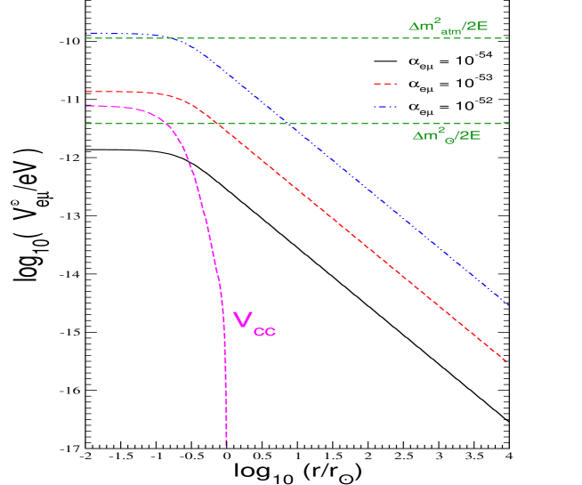
Figure 1: Comparison of the MSW potential $V_{cc}$ and the LR potential $V_{e\mu}^{\odot}$ due to the solar electrons from the solar core all the way to the Earth ($r/r_{\odot}\approx 215$) and beyond. The $(\Delta m^{2}/2E)$ values corresponding to $E=10$ MeV are also shown.

The contribution $\tilde{V}_{e\beta}^{E}$ of the electrons inside the Earth can be calculated in a similar fashion. Roughly, one finds that at the Earth surface,

$$\frac{{V}_{e\beta}^{E}}{V_{e\beta}^{\odot}}\approx\frac{M_{E}}{M_{\odot}}\frac{R_{es}}{R_{E}}\approx 10^{-1}\;,$$ (8)

where $M_{\odot}(M_{E})$ and $R_{es}(R_{E})$ respectively refer to the mass of the Sun (Earth) and the Earth-Sun distance (radius of the Earth). Thus the solar long range potential dominates over the terrestrial contribution and we will neglect the latter. As long as $R_{LR}\ll R_{\rm gal}$, this is the dominant potential affecting the propagation of solar neutrinos.

When $R_{LR}\mathrel{\hbox to0.0pt{\lower 4.0pt\hbox{\hskip 1.0pt$\sim$}\hss}\raise 1.0pt\hbox{$>$}}R_{\rm gal}$, the collective potential due to all the electrons in the galaxy may become significant. The mass of the Milky Way is (0.6 – 3.0) $\times 10^{12}$ solar masses, which is mostly concentrated in the center of the galaxy. The baryonic contribution to the galactic mass may be estimated to be ${\cal O}(10\%)$. The center of the galaxy is $\sim$ 10 kpc away from the Sun. We denote the galactic contribution to the potential $V_{e\beta}$ as

$$V_{e\beta}^{\rm gal}=b~{}\alpha_{e\beta}~{}\frac{N^{0}_{e,{\rm gal}}}{R^{0}_{\rm gal}}\;,$$ (9)

where $N^{0}_{e,{\rm gal}}$ is taken to be $10^{12}N_{e}^{\odot}$ and $R^{0}_{\rm gal}$ to be 10 kpc. The net LR potential is $V_{e\beta}=V_{e\beta}^{\odot}+V_{e\beta}^{\rm gal}$. The parameter $b$ takes care of our ignorance about the distribution of the baryonic mass in our galaxy. With $R_{LR}\mathrel{\hbox to0.0pt{\lower 4.0pt\hbox{\hskip 1.0pt$\sim$}\hss}\raise 1.0pt\hbox{$>$}}R_{\rm gal}$, we expect $0.05<b\mathrel{\hbox to0.0pt{\lower 4.0pt\hbox{\hskip 1.0pt$\sim$}\hss}\raise 1.0pt\hbox{$<$}}1$. The value of $b$ may be smaller if $R_{LR}$ is smaller. Clearly, $b=0$ would have the same effect as $R_{LR}\ll R_{\rm gal}$. With $b\neq 0$, the constraints on $\alpha$ become stronger, as will be demonstrated in Sec. V.

The screening length due to the antineutrinos present in the cosmic neutrino background is a few hundred kpc for $m_{\nu}\sim 0.1$ eV screening . Therefore, for the galactic scale, the screening plays no significant role. Over the Sun-Earth distance, even the possible local screening effects would be too small to have any effect mj1 .

In addition to the altered resonance structure inside and outside the Sun, the mixing angles at the Earth also differ from the corresponding vacuum values, with the result that both the solar and the KamLAND neutrinos get affected by the LR potential. An important point to note is that this potential gives unequal contributions to two flavors ($e$ and $\mu$ or $\tau$) simultaneously unlike in case of the charged current which contributes only to the electrons. The third flavor gets no contribution. As a consequence of this, the inclusion of three generations in the solar analysis becomes necessary.

The appropriate Hamiltonian in the flavor basis describing the neutrino propagation can be written as

$$H_{f}=R_{23}(\theta_{23})R_{13}(\theta_{13})R_{12}(\theta_{12})H_{0}R_{12}^{T}(\theta_{12})R_{13}^{T}(\theta_{13})R_{23}^{T}(\theta_{23})+V\;,$$ (10)

where $H_{0}$ refers to the effective Hamiltonian in the mass basis, and $R_{ij}$’s are the rotation matrices in the $i$-$j$ plane. Since the absolute masses of neutrinos play no part in the oscillation phenomena, we can take the neutrino mass eigenvalues in vacuum to be $0,\sqrt{\Delta m^{2}_{21}},\sqrt{\Delta m^{2}_{32}}$ respectively, leading to

$$H_{0}={\rm Diag}(0,\Delta_{21},\Delta_{32})\;,$$ (11)

where $\Delta_{21}\equiv\Delta m^{2}_{21}/(2E)$ and $\Delta_{32}\equiv\Delta m^{2}_{32}/(2E)$. The rotation angles $\theta_{23}$ and $\theta_{12}$ are the vacuum mixing angles describing the atmospheric and the solar neutrino oscillations respectively, whereas $\theta_{13}$ is the third “Chooz” mixing angle. We have assumed that no CP violation enters into picture here.

The matrix $V$ in (10) describes the combined contribution of the charge weak currents as well as the long range forces. Explicitly,

$$V={\rm Diag}(V_{cc}+V_{e\mu},-V_{e\mu},0)\;.$$ (12)

The neutrino propagation is described by eq. (10). The corresponding antineutrino propagation is obtained by the replacement $V\rightarrow-V$.

III Masses, Mixings and Resonances of Solar Neutrinos

In order to analyze the propagation of solar neutrinos, we rewrite eq. (10) explicitly as

$$H_{f}=\Delta_{32}\left(\begin{array}[]{ccc}xs_{12}^{2}+y_{c}+y_{e\mu}&xc_{12}s_{12}c_{23}+s_{13}s_{23}&-xc_{12}s_{12}s_{23}-s_{13}c_{23}\\ xc_{12}s_{12}c_{23}+s_{13}s_{23}&s_{23}^{2}+xc_{12}^{2}c_{23}^{2}-y_{e\mu}&c_{23}s_{23}(1-xc_{12}^{2})\\ -xc_{12}s_{12}s_{23}-s_{13}c_{23}&c_{23}s_{23}(1-xc_{12}^{2})&c_{23}^{2}+xc_{12}^{2}s_{23}^{2}\\ \end{array}\right)\;,$$ (13)

where

$$x\equiv\frac{\Delta_{21}}{\Delta_{32}}\approx 0.03~{}~{},~{}~{}y_{c}\equiv\frac{V_{cc}}{\Delta_{32}}=\frac{2EV_{cc}}{\Delta m_{32}^{2}}~{}~{},~{}~{}y_{e\mu}\equiv\frac{V_{e\mu}}{\Delta_{32}}=\frac{2EV_{e\mu}}{\Delta m_{32}^{2}}\;,$$ (14)

and $s_{ij}\equiv\sin\theta_{ij},c_{ij}\equiv\cos\theta_{ij}$. Since $\theta_{13}$ is small ($\theta_{13}<0.2$ lma ), we have kept terms to only linear order in $s_{13}$.

Eq.(13) can be diagonalized through the unitary matrix

$$U_{m}\equiv R_{23}(\theta_{23m})R_{13}(\theta_{13m})R_{12}(\theta_{12m})$$ (15)

such that

$$U_{m}^{T}H_{f}U_{m}=\frac{1}{2E}{\rm Diag}(m_{1m}^{2},m_{2m}^{2},m_{3m}^{2})\;.$$ (16)

The smallness of $x$ and $s_{13}$ can be used to approximately determine the matter dependent mixing angles of $U_{m}$ to the leading order in these parameters. The angle $\theta_{23m}$ follows from the lower right $2\times 2$ block in (13):

$$\tan 2\theta_{23m}\approx\frac{\sin 2\theta_{23}(1-xc_{12}^{2})}{\cos 2\theta_{23}(1-xc_{12}^{2})+y_{e\mu}}\;.$$ (17)

The subsequent diagonalization leads to

$$\tan 2\theta_{13m}\approx\frac{2~{}(xs_{12}c_{12}S+s_{13}C)}{C^{2}+x(c_{12}^{2}S^{2}-s_{12}^{2})-y_{c}-y_{e\mu}(1+\sin^{2}\theta_{23m})}\;,$$ (18)

where $S\equiv\sin(\theta_{23m}-\theta_{23})$ and $C\equiv\cos(\theta_{23m}-\theta_{23})$.

As long as the denominator in eq. (18) does not vanish (which happens only in a very narrow range of $y_{e\mu}$ near $y_{e\mu}\approx 2/3$), we can take $\theta_{13m}\sim{\cal O}(x,s_{13})$. Neglecting terms that are quadratic or higher order in ${\cal O}(x,s_{13})$, the effective Hamiltonian in the new basis (after the 2-3 and 1-3 rotation) becomes

$$H_{f^{\prime\prime}}\approx\Delta_{32}\left(\begin{array}[]{ccc}xs_{12}^{2}+y_{c}+y_{e\mu}&xc_{12}s_{12}C-s_{13}S&0\\ xc_{12}s_{12}C-s_{13}S&S^{2}+xc_{12}^{2}C^{2}-y_{e\mu}c_{23m}^{2}&0\\ 0&0&C^{2}+xc_{12}^{2}S^{2}-y_{e\mu}s_{23m}^{2}\\ \end{array}\right)\;,$$ (19)

so that a 1-2 rotation through an angle $\theta_{12m}$, given by

$$\tan 2\theta_{12m}\approx\frac{2~{}(xs_{12}c_{12}C-s_{13}S)}{S^{2}+x(c_{12}^{2}C^{2}-s_{12}^{2})-y_{c}-y_{e\mu}(1+\cos^{2}\theta_{23m})}\;,$$ (20)

completes the diagonalization. The neutrino masses are given as

$$m_{1m}^{2} \approx \Delta_{32}E\left[x(c_{12}^{2}C^{2}+S^{2})+y_{c}+y_{e\mu}\sin^{2}\theta_{23m}+S^{2}-D^{1/2}\right]~{},$$

$$m_{2m}^{2} \approx \Delta_{32}E\left[x(c_{12}^{2}C^{2}+S^{2})+y_{c}+y_{e\mu}\sin^{2}\theta_{23m}+S^{2}+D^{1/2}\right]~{},$$

$$m_{3m}^{2} = 2\Delta_{32}E(C^{2}+xc_{12}^{2}S^{2}-y_{e\mu}\sin^{2}\theta_{23m})\;,$$ (21)

where

$$D=\left[S^{2}+x(c_{12}^{2}C^{2}-s_{12}^{2})-y_{c}-y_{e\mu}(1+\cos^{2}\theta_{23m})\right]^{2}+4~{}(xs_{12}c_{12}C-s_{13}S)^{2}\;.$$ (22)

The above analytical results can be verified by the exact numerical results in Fig. 2 where we show the angles and $m_{i}^{2}$ values in matter for different values of $\alpha$ for normal as well as inverted hierarchy.

In this and the next section, we analyze the case $R_{LR}\ll R_{\rm gal}$, so that the potential $V_{e\mu}$ is as shown in Fig. 1. As is apparent from the figure, the maximum value of $y_{e\mu}$ is given by

$$\frac{(y_{e\mu})_{max}}{\alpha}\approx 1.2\times 10^{52}\left(\frac{E}{10~{}{\rm MeV}}\right)$$ (23)

for the best fit values of the atmospheric parameters. Thus, at $E=10$ MeV, we have $y_{e\mu}\approx 0.1$ for $\alpha=10^{-53}$. The left column in Fig. 2 then corresponds to the range of $\alpha$ where $(y_{e\mu})_{max}\ll 1$, and the right column corresponds to $(y_{e\mu})_{max}>1$.

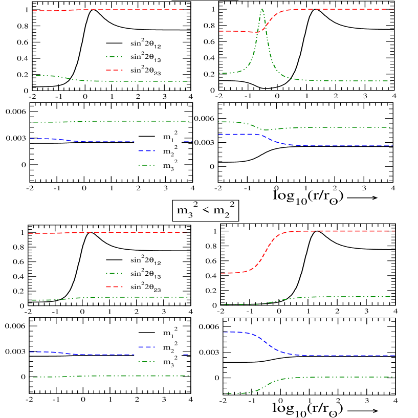
Figure 2: The angles and $m_{i}^{2}$ values in matter for solar neutrinos for $E=10$ MeV, in the case $R_{LR}\ll R_{\rm gal}$. The $m_{i}^{2}$ values are correct up to an additive constant, so that only their relative values have a physical significance.

The propagation of solar neutrinos is qualitatively and quantitatively different depending on whether $(y_{e\mu})_{max}$ is large enough to cause resonant enhancement of $\theta_{13m}$ in (18). The resonance occurs when $\alpha\mathrel{\hbox to0.0pt{\lower 4.0pt\hbox{\hskip 1.0pt$\sim$}\hss}\raise 1.0pt\hbox{$>$}}10^{-52}$. We therefore consider the two cases $\alpha\mathrel{\hbox to0.0pt{\lower 4.0pt\hbox{\hskip 1.0pt$\sim$}\hss}\raise 1.0pt\hbox{$<$}}10^{-52}$ and $\alpha\mathrel{\hbox to0.0pt{\lower 4.0pt\hbox{\hskip 1.0pt$\sim$}\hss}\raise 1.0pt\hbox{$>$}}10^{-52}$ separately in the next two subsections.

III.1 For $\alpha\mathrel{\hbox to0.0pt{\lower 4.0pt\hbox{\hskip 1.0pt$\sim$}\hss}\raise 1.0pt\hbox{$<$}}10^{-52}$

For $\alpha\ll 10^{-52}$, we have $y_{e\mu}\ll 1$ and the atmospheric mixing angle gets only a small correction from the matter effects. Writing $\theta_{23m}=\theta_{23}+\delta\theta_{23}$, we see that $\delta\theta_{23}\approx-y_{e\mu}\sin 2\theta_{23}/2$ and $\theta_{23m}$ remains close to its vacuum value, $\theta_{23m}\approx\pi/4$. With a higher $\alpha$ value, the deviation $\delta\theta_{23}$ becomes appreciable and results in the reduction of $\sin^{2}2\theta_{23m}$ as shown in Fig. 2.

The angle $\theta_{13m}$ has contributions from two sources: from finite $\theta_{13}$ in vacuum as well as the additional contribution from the term $xs_{12}c_{12}S$. The latter is doubly suppressed because of the smallness of $x$ as well as $S\approx\delta\theta_{23}$, and can be neglected as long as $s_{13}>xS$ . One may then take $\theta_{13m}\sim{\cal O}(s_{13})$ since the resonant enhancement of $\theta_{13m}$ anyway does not occur for $\alpha<10^{-52}$.

In the limit $\theta_{13m}\to 0$, the third mass eigenstate decouples and the scenario reduces to 2$\nu$ mixing, as can be seen from eq. (19). However, note that the effective matter potential is

$${\cal V}_{12}\approx V_{cc}+V_{e\mu}(1+\cos^{2}\theta_{23m})\;,$$ (24)

and not $V_{cc}+2V_{e\mu}$ as would have been taken in a naive 2-generation analysis. Thus, the effect of the third neutrino and its mixing is inescapable here. However, it only appears through the factor $(1+c_{23m}^{2})$ in eq. (24), and the mass of the third neutrino or the mass hierarchy is immaterial for the effective 2$\nu$ analysis. This may be verified from the left column of fig. 2.

The most important effect of the LR potential is for the solar angle. Eq. (20) gives the resonance condition

$$\Delta m_{21}^{2}\cos 2\theta_{12}\approx 2E\left[V_{cc}+V_{e\mu}(1+\cos^{2}\theta_{23m})\right]\;,$$ (25)

which differs from the MSW condition by an addition of the term involving $V_{e\mu}$. For $\alpha\mathrel{\hbox to0.0pt{\lower 4.0pt\hbox{\hskip 1.0pt$\sim$}\hss}\raise 1.0pt\hbox{$>$}}10^{-53}$, the $V_{e\mu}$ contribution dominates over $V_{cc}$ and changes the MSW resonance picture significantly. The resonance is shifted away from the center as $\alpha$ increases. Eventually for some value of $\alpha$ the resonance gets shifted outside the Sun where its behavior is solely determined by the LR potential. For $\alpha>10^{-53}$, neutrinos with $E=10$ MeV encounter resonance outside the Sun in case of the best fit values of the neutrino mass parameters obtained in the standard analysis lma .

Addition of the $V_{e\mu}(1+\cos^{2}\theta_{23m})$ term to $V_{cc}$ makes the variation of the total potential smoother than the normal MSW potential with the result that the transition becomes more adiabatic than the corresponding case without the LR. In particular, when the resonance occurs outside the Sun then $V_{e\mu}^{\odot}\sim\frac{\alpha N_{e}^{\odot}}{r}$ and the adiabaticity parameter at the resonance is given by

$$\gamma_{L} \equiv \frac{\Delta m_{12}^{2}}{2E}\frac{\sin^{2}2\theta_{12}}{\cos 2\theta_{12}}\left|\frac{1}{{\cal V}_{12}}\frac{d{\cal V}_{12}}{dr}\right|_{res}^{-1}$$ (26)

$$\approx \alpha_{e\mu}N_{e}^{\odot}\tan^{2}2\theta_{12}(1+\cos^{2}\theta_{23})~{}\approx 1.4\times 10^{58}~{}\alpha_{e\mu}\;.$$

The value of $\gamma_{L}$ is independent of the neutrino masses, energy and position of the resonance and is solely determined by $\alpha$ and the vacuum mixing angles. For the standard values of the latter, the resonance is found to be highly adiabatic: $\gamma_{L}\gg 1$ for $\alpha>10^{-57}$. In general, if $P_{L}(E)\equiv exp(-\pi\gamma_{L}/2)$ is the probability that $\nu_{1m}$ and $\nu_{2m}$ convert to each other while passing through the resonance, the net survival probability of $\nu_{e}$ is

$$P_{ee}(E) = (1-P_{L})\cos^{2}\theta_{13P}\cos^{2}\theta_{12P}\cos^{2}\theta_{13E}\cos^{2}\theta_{12E}$$ (27)

$$+ P_{L}\cos^{2}\theta_{13P}\sin^{2}\theta_{12P}\cos^{2}\theta_{13E}\cos^{2}\theta_{12E}$$

$$+ (1-P_{L})\cos^{2}\theta_{13P}\sin^{2}\theta_{12P}\cos^{2}\theta_{13E}\sin^{2}\theta_{12E}$$

$$+ P_{L}\cos^{2}\theta_{13P}\cos^{2}\theta_{12P}\cos^{2}\theta_{13E}\sin^{2}\theta_{12E}$$

$$+ \sin^{2}\theta_{13P}\sin^{2}\theta_{13E}\;.$$

Here $\theta_{ijP}$ and $\theta_{ijE}$ are the values of $\theta_{ijm}$ at the neutrino production point and at the Earth respectively. The energy dependence of $P_{L}$ as well as all the angles is implicit. Note that since $\theta_{13P},\theta_{13E}\sim{\cal O}(\theta_{13})$, the last term may be neglected if we neglect terms of ${\cal O}(\theta_{13}^{4})$ or smaller.

III.2 For $\alpha{\mathrel{\hbox to0.0pt{\lower 4.0pt\hbox{\hskip 1.0pt$\sim$}\hss}\raise 1.0pt\hbox{$>$}}}10^{-52}$

For $\alpha\sim 10^{-52}$, the value of $y_{e\mu}$ is large enough so that $\sin^{2}2\theta_{23m}$ gets unacceptably suppressed through eq. (17). This also suppresses the atmospheric neutrino flux and results in the bounds on $\alpha$ discussed in mj1 .

For solar neutrinos, the $\nu_{1m}$-$\nu_{2m}$ resonance as described in the previous section occurs, but in addition the angle $\theta_{13m}$ gets resonantly enhanced when

$$C^{2}+x(S^{2}c_{12}^{2}-s_{12}^{2})-y_{c}-y_{e\mu}(1+\sin^{2}\theta_{23m})\approx 0\;.$$ (28)

This happens when $y_{e\mu}\approx 2/3$. The sign of $y_{e\mu}$ also needs to be positive, so the resonance occurs only for normal hierarchy. For the inverted hierarchy, there is no resonance for $\nu_{e}$ and eq. (27) gives the correct expression for their survival probability.

In the resonance region, the effective Hamiltonian matrix (10) can no longer be diagonalized through the simple procedure described in the beginning of Sec. III, and the mixing angles have to be computed numerically. However, this happens only in a small range of $y_{e\mu}$ around $y_{e\mu}\approx 2/3$: the width of the resonance region may be estimated to be $\delta y_{e\mu}\approx(2/3)s_{13}$. The expressions (20)-(22) are valid everywhere outside this region.

The $\theta_{13m}$ enhancement corresponds to the $\nu_{2m}$-$\nu_{3m}$ level crossing, with an effective potential

$${\cal V}_{23}=V_{cc}+V_{e\mu}(1+\sin^{2}\theta_{23m})\;.$$ (29)

When the hierarchy is normal, only a fraction of the $\nu_{e}$ that are produced mainly as $\nu_{2m}$ inside the Sun survive the $\nu_{2m}$-$\nu_{3m}$ resonance. The adiabaticity at this resonance, which strongly depends on $\theta_{13}$, affects the net survival probability of $\nu_{e}$:

$$P_{ee}(E) = \cos^{2}\theta_{13P}\cos^{2}\theta_{12P}\cos^{2}\theta_{13E}\cos^{2}\theta_{12E}$$ (30)

$$+ (1-P_{H})\cos^{2}\theta_{13P}\sin^{2}\theta_{12P}\cos^{2}\theta_{13E}\sin^{2}\theta_{12E}$$

$$+ P_{H}\sin^{2}\theta_{13P}\cos^{2}\theta_{13E}\sin^{2}\theta_{12E}$$

$$+ (1-P_{H})\sin^{2}\theta_{13P}\sin^{2}\theta_{13E}$$

$$+ P_{H}\cos^{2}\theta_{13P}\sin^{2}\theta_{12P}\sin^{2}\theta_{13E}\;,$$

where $P_{H}(E)$ is the probability that $\nu_{2m}$ converts to $\nu_{3m}$ after traversing through this resonance.

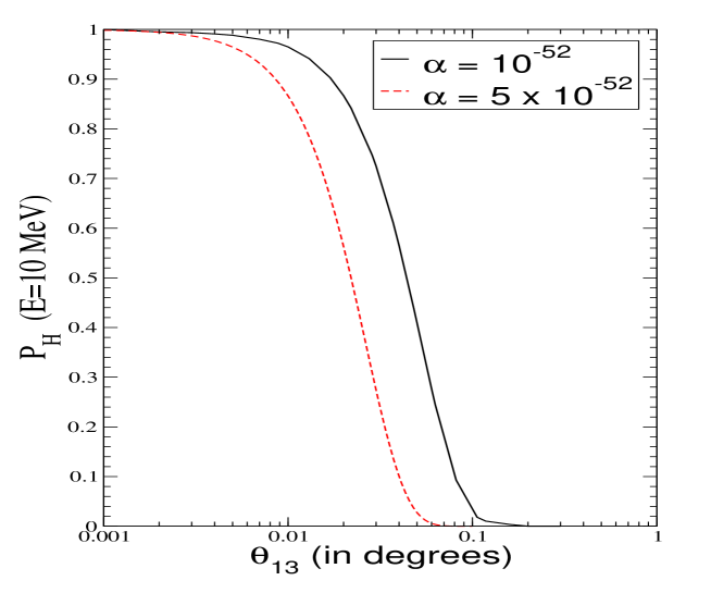
Figure 3: $\theta_{13}$ dependence of $P_{H}$ for various values of $\alpha$ for $E=10$ MeV in the case $R_{LR}\ll R_{\rm gal}$.

Here we have used the earlier result that for $\alpha\mathrel{\hbox to0.0pt{\lower 4.0pt\hbox{\hskip 1.0pt$\sim$}\hss}\raise 1.0pt\hbox{$>$}}10^{-52}$ the $\nu_{1m}-\nu_{2m}$ resonance is outside the Sun and is always adiabatic [see eq. (26)]. The energy dependence of $P_{H}$ as well as all the angles is implicit.

The value of $P_{H}$ is given by

$$P_{H}\approx\exp\left[-\frac{\pi}{2}\left|\frac{m_{3}^{2}-m_{2}^{2}}{2E~{}d\theta_{13m}/dr}\right|_{\rm res}\right]\;.$$ (31)

Clearly, if $P_{H}\approx 0$, the expression (30) reduces to (27), and the results of the 2$\nu$ analysis stay valid. In general $P_{H}\approx 0$ at high values of $\theta_{13}$. In Fig. 3, we show the $\theta_{13}$ dependence of $P_{H}$ for various values of $\alpha$ for $E=10$ MeV. At $\alpha=10^{-52}$, the value of $P_{H}>0.1$ for $\theta_{13}<0.08^{\circ}$, which is when the survival probability is affected significantly. For larger $\alpha$, the value of $P_{H}$ becomes significant for lower $\theta_{13}$ values. In the range where $0.1<P_{H}<0.9$ (the semi-adiabatic range), $P_{H}$ is also highly energy dependent, as can be seen from (31).

The analytic discussion above reveals that the LR potential makes important contribution to the solar neutrino problem and a detailed numerical analysis is needed to obtain constraints on this potential. We turn to this analysis in the next section.

IV Constraints from solar neutrinos and KamLAND

To find the best fit values of the oscillation parameters and $\alpha$ from a statistical analysis of the experimental data, we employ the ${\chi^{2}}$ minimization technique with covariance approach for the errors. For analysis of the total event rate data from all the experiments, the ${\chi^{2}}$ function is defined as

$${\chi^{2}}_{\rm rates} = \sum_{i,j=1}^{N_{\rm expt}}(P^{\rm th}_{i}-P^{\rm expt}_{i})\left[(\sigma_{ij}{}^{rates})^{2}\right]^{-1}(P^{\rm th}_{j}-P^{\rm expt}_{j})\;,$$ (32)

where P${}_{i}^{\xi}$ ($\xi$ = th or expt) denotes the total event rate for the $i^{\rm th}$ experiment. Both the theoretical and experimental values of the fitted quantities are normalized relative to the standard solar model (SSM) predictions. The error matrix $(\sigma_{ij}{}^{rates})^{2}$ contains the experimental and theoretical uncertainties along with their correlations. Theoretical uncertainties include the uncertainties in the capture cross sections, which are uncorrelated between different experiments and the astrophysical uncertainties from the SSM predictions which are correlated between different experiments. The correlations are being evaluated using the procedure of ana2g_lisicorr .

For the analysis of any spectral data (recoil energy spectra or zenith angle spectra), the ${\chi^{2}}$ is defined as

$${\chi^{2}}_{\rm spec} = \sum_{i,j=1}^{N_{\rm bins}}(S^{\rm th}_{i}-S^{\rm expt}_{i})\left[(\sigma_{ij}{}^{spec})^{2}\right]^{-1}(S^{\rm th}_{j}-S^{\rm expt}_{j})\;,$$ (33)

where S${}_{i}^{\xi}$ ($\xi$=th or expt) is the number of events in the $i^{\rm th}$ bin of the spectrum. The error matrix $(\sigma_{ij}{}^{spec})^{2}$ for the spectral data includes the statistical error, correlated and uncorrelated systematic errors in the different bins and the error due to the calculation of the neutrino energy spectrum from SSM.

For a global analysis of the solar data – rates from Cl, Ga experiment, spectral data from SuperKamiokande (SK) and Sudbury Neutrino Observatory (SNO): both D₂O and salt phase, and KamLAND data – the relevant ${\chi^{2}}$ is given by

$${\chi^{2}}={\chi^{2}}_{\rm Cl,Ga~{}rates}+{\chi^{2}}_{\rm SK~{}spec}+{\chi^{2}}_{\rm SNO~{}spec}+{\chi^{2}}_{\rm KamLAND}\;.$$ (34)

Note that only solar neutrino observations would not have been able to put strong constraints on $\alpha$: as long as there is no $\nu_{2m}$-$\nu_{3m}$ level crossing and the $\nu_{1m}$-$\nu_{2m}$ resonance is adiabatic, the net $\nu_{e}$ survival probability (27) is a function of $\Delta m_{12}^{2}/\alpha$ for a large $\alpha$, i.e. for $V_{cc}<<V_{e\mu}$. As a result, one can fit the solar data by increasing the value of $\Delta m_{12}^{2}$ when $\alpha$ is increased and a strong bound on $\alpha$ would not follow.

However, the data from KamLAND restricts $\Delta m^{2}_{21}$ to a very small range and plays a crucial role in constraining $\alpha$. We use eqs. (27) and (30) for the survival probability of solar neutrinos. The $\bar{\nu_{e}}$ survival probability in KamLAND is given by

$$P_{\bar{e}\bar{e}}^{KL} = 1-\cos^{4}\theta_{13}\left[\sin^{2}2\theta_{12}\sin^{2}\left(\frac{\Delta m^{2}_{21}L}{4E}\right)\right]-\sin^{2}2\theta_{13}\sin^{2}\left(\frac{\Delta m^{2}_{31}L}{4E}\right)$$ (35)

$$+\sin^{2}2\theta_{13}\sin^{2}\theta_{12}\left[\sin^{2}\left(\frac{\Delta m^{2}_{31}L}{4E}\right)-\sin^{2}\left(\frac{(\Delta m^{2}_{31}-\Delta m^{2}_{21})L}{4E}\right)\right]\;,$$

where all the mass squared differences and the angles are measured at the Earth for antineutrinos. Note that for antineutrinos, the sign of $V_{cc}$ as well as $V_{e\mu}$ is reversed with respect to the neutrinos.

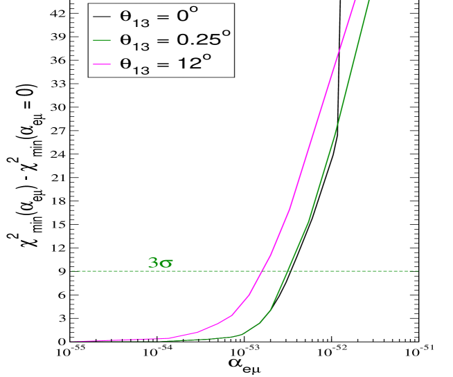
Figure 4: $\Delta\chi^{2}\equiv\chi^{2}(\alpha_{e\mu})-\chi^{2}(\alpha_{e\mu}=0)$ values for different $\theta_{13}$ values, in the case $R_{LR}\ll R_{\rm gal}$.

In Fig. 4, we show the $\Delta\chi^{2}$ values as a function of the parameter $\alpha$ for various $\theta_{13}$ values. The best fit values for the solar parameters are always observed to lie in the LMA range with vanishing $\alpha_{e\mu}$ giving the best fit. For $\alpha<10^{-52}$, the value of $\chi^{2}$ is minimum for $\theta_{13}=0^{\circ}$, which is consistent with the observation that $\theta_{13}=0^{\circ}$ also gives the best fit to the solar and KamLAND data when the LR forces are not taken into account lma . When $\alpha>10^{-52}$, a strong energy dependence in the survival probability is introduced for $\theta<0.8^{\circ}$ through $P_{H}$, so that the $\chi^{2}$ values for extremely low $\theta_{13}$ values become large. In this region, the lowest $\chi^{2}$ is found to be at values of $\theta_{13}$ that are small, but still keep $P_{H}\approx 0$. We have shown $\chi^{2}$ corresponding to such a $\theta_{13}$ in the figure.

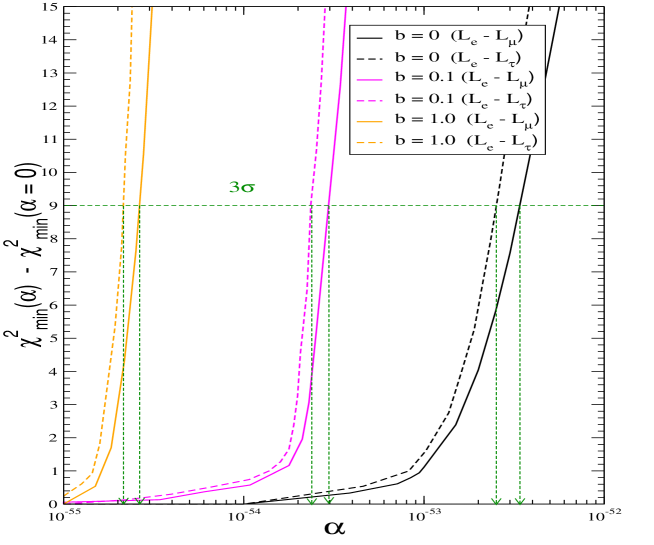
Figure 5: $\Delta\chi^{2}$ values and limits for the $L_{e}-L_{\mu}$ as well as $L_{e}-L_{\tau}$ symmetry, with $\theta_{13}=0^{\circ}$. The case $R_{LR}\ll R_{\rm gal}$ is represented by $b=0$ and higher $b$ values correspond to larger contributions from galactic electrons (see Sec. V).

The bounds on $\alpha$ should therefore be, strictly speaking, $\theta_{13}$-dependent. However, the region $\alpha>10^{-52}$, where the $\theta_{13}$ dependence from $P_{H}$ starts coming into picture, is excluded to more than 3$\sigma$ as can be seen from Fig. 4. Therefore the constraints on $\alpha$ by using $\theta_{13}=0^{\circ}$ are the most conservative ones, and we quote the upper bounds on $\alpha$ obtained by taking $\theta_{13}=0^{\circ}$. These limits are shown in Fig. 5: the $3\sigma$ limit corresponding to the one-parameter fit is

$$\alpha_{e\mu}<3.4\times 10^{-53}\;.$$ (36)

The corresponding limit in the $L_{e}-L_{\tau}$ case (see Appendix A) is

$$\alpha_{e\tau}<2.5\times 10^{-53}\;.$$ (37)

The bounds are independent of whether the neutrino mass hierarchy is normal or inverted.

V The long range potential due to galactic electrons

The collective contribution of all the electrons in the galaxy to the LR potential in the solar system may be parametrized in general as given in eq. (9). The net potential $V_{e\mu}\equiv V_{e\mu}^{\odot}+V_{e\mu}^{\rm gal}$ is shown in Fig. 6 for various values of $b$ and $\alpha$. Clearly, larger the value of $b$ or $\alpha$, larger the value of $V_{e\mu}$. Also, note that the value of $V_{e\mu}$ near the earth is approximately the same as $V_{e\mu}^{\rm gal}$, since $V_{e\mu}^{\odot}$ keeps on decreasing as one travels towards the Earth, whereas $V_{e\mu}^{\rm gal}$ is a constant over the scale of the solar system.

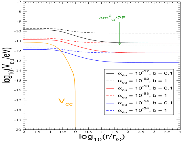
Figure 6: The net potential $V_{e\mu}\equiv V_{e\mu}^{\odot}+V_{e\mu}^{\rm gal}$ for various values of $b$ and $\alpha$.

With our understanding of the effects of the LR potential on neutrino masses, mixings and resonances obtained in Sec. III, the following observations may be made:
(i) For $V_{e\mu}^{\rm gal}\gg\Delta m^{2}_{\odot}/(2E)$, there is no MSW resonance that is essential for a good fit to the solar neutrino data. Therefore, larger values of $b$ and $\alpha$ ($b\alpha\mathrel{\hbox to0.0pt{\lower 4.0pt\hbox{\hskip 1.0pt$\sim$}\hss}\raise 1.0pt\hbox{$>$}}10^{-53}$) are expected to be ruled out from the global fit.
(ii) For $V_{e\mu}^{\rm gal}\ll\Delta m^{2}_{\rm solar}/(2E)$, the matter potential $V_{CC}$ dominates inside the Sun, and the standard picture of the neutrino flavor conversions inside the Sun is not affected. Therefore, smaller values of $b$ and $\alpha$ ($b\alpha\mathrel{\hbox to0.0pt{\lower 4.0pt\hbox{\hskip 1.0pt$\sim$}\hss}\raise 1.0pt\hbox{$<$}}10^{-55}$) should be allowed.
(iii) For the intermediate values of $V_{e\mu}^{\rm gal}$, the situation depends strongly on whether the potential profile near the MSW resonance is dominated by $V_{CC}$ or $V_{e\mu}^{\rm gal}$. In the former case, the resonance is adiabatic for $E>5$ GeV and only partially adiabatic for lower energies, which gives a good fit to the data. In the latter case, however, the resonance tends to be adiabatic even for low energies, so that the radiochemical data will disfavor the solution.

The value of $b$ is expected to be in the range $0.05<b<0.5$ (see Sec. II). The $\Delta\chi^{2}$ values as a function of $\alpha$ for $b=0~{}(i.e.\ R_{LR}\ll R_{\rm gal})$, $b=0.1$ and $b=1$ are shown in Fig. 5. The 3$\sigma$ constraints for $L_{e}-L_{\mu}$ are

$$\alpha_{e\mu}<2.9\times 10^{-54}~{}~{}(b=0.1)\quad,\quad\alpha_{e\mu}<2.6\times 10^{-55}~{}~{}(b=1)$$ (38)

and for $L_{e}-L_{\tau}$, they are

$$\alpha_{e\tau}<2.3\times 10^{-54}~{}~{}(b=0.1)\quad,\quad\alpha_{e\tau}<2.1\times 10^{-55}~{}~{}(b=1)\;.$$ (39)

Clearly, the constraints get stronger as $b$ increases. The most conservative constraints are therefore with $b=0$, as calculated in Sec. IV.

VI Summary and conclusions

Flavor-dependent long range leptonic forces, like those mediated by the $L_{e}-L_{\mu}$ or $L_{e}-L_{\tau}$ gauge bosons, constitute a minimal extension of the standard model that preserves its renormalizability. The flavor dependent potentials produced by these forces influence neutrino oscillations. The effects of these are quite significant in spite of the very strong constraints on the couplings of such forces from astronomical observations or Eötvös type laboratory experiments. We have performed a detailed study of specific effects of these forces in the solar neutrino and the KamLAND experiments.

It was found that the new forces change the standard MSW picture in a qualitatively different way which ultimately results in a strong bound on the couplings of these forces. We have developed a detailed formalism to describe these effects and have used it to obtain bounds on the couplings from the statistical analysis of the experimental data. It was shown that the mixing among all three generations needs to be taken into account because of the fact that the $L_{e}-L_{\mu,\tau}$ gauge bosons couple to two out of three flavors at a time. The changes which result in the MSW analysis were studied both analytically as well as numerically in the case $R_{LR}\ll R_{\rm gal}$, when the galactic electron contribution to the LR potential may be neglected compared with the solar electron contribution.

A qualitatively new effect studied in detail is the possible resonant enhancement of $\theta_{13}$. In the standard MSW picture, a non-zero but small $\theta_{13}$ can only give sub-leading corrections. In contrast, the long range potential can resonantly amplify $\theta_{13}$ if $\alpha\mathrel{\hbox to0.0pt{\lower 4.0pt\hbox{\hskip 1.0pt$\sim$}\hss}\raise 1.0pt\hbox{$>$}}10^{-52}$ and the neutrino mass hierarchy is normal. The global analysis of the solar data however constrains $\alpha<10^{-52}$. As a result, the resonance enhancement of $\theta_{13}$ does not take place in the solar case. But this resonance effect can play an important role in other environments, e.g. inside a supernova. See Appendix B for details.

A global $\chi^{2}$ analysis of all the solar neutrino and KamLAND data was performed to constrain the coupling $\alpha$. The solar data alone are found to be inadequate in constraining $\alpha$: one could always fit these data by appropriate change in $\Delta m_{12}^{2}$ compared to the standard LMA values. This does not remain true when the KamLAND results are included. A significant bound on $\alpha$ is obtained by combining the solar and KamLAND results. The conservative $3\sigma$ bounds follow when $\theta_{13}=0$:

$$\alpha_{e\mu}<3.4\times 10^{-53}\quad,\quad\alpha_{e\tau}<2.5\times 10^{-53}\;.$$ (40)

These bounds are stronger by more than one order of magnitude than the ones in eq. (3) following from the analysis of the atmospheric neutrino data.

A much stronger bound on $\alpha$, namely $\alpha<6.4\times 10^{-54}$, was quoted in masso purely from the solar neutrino results. This was not based on the detailed statistical analysis as presented here, but was obtained under the assumption that even in the presence of $\alpha$ the $\Delta m_{12}^{2}$ and $\theta_{12}$ should lie within their 95% C. L. range obtained in the standard LMA solution. This assumption need not a priori be true. In fact as discussed here, the solar neutrino results by themselves cannot be used to constrain $\alpha$, so the detailed analysis as done here is required. An analysis similar to ours has recently been carried out in garcia which has reported bounds on couplings of the vector and non-vector long range forces. The resulting bound on $\alpha$ in the former case is similar to ours. However, they assume one mass scale dominance, neglecting the mass eigenstate $\nu_{3}$ altogether. As shown in this paper, in the presence of the LR potential, $\nu_{3}$ affects the solar neutrino survival probability significantly even when $\theta_{13}$ is vanishingly small. Moreover, the galactic contribution has not been included in the analysis of garcia even when the range of the force is more than our distance from the galactic center.

When $R_{LR}\mathrel{\hbox to0.0pt{\lower 4.0pt\hbox{\hskip 1.0pt$\sim$}\hss}\raise 1.0pt\hbox{$>$}}R_{\rm gal}$, the collective contribution of all the electrons in the galaxy to the LR potential becomes significant. This gives more stringent constraints on the value of $\alpha$, which also depend on the distribution of baryonic mass within the galaxy. We parametrize our ignorance about this with a parameter $b$ (expected to lie between 0.05 and 1 with conservative estimates) and perform global fits to constrain $\alpha$ for fixed $b$ values. We obtain $\alpha_{e\mu}<2.9\times 10^{-54}$ for $b=0.1$ and $\alpha_{e\mu}<2.6\times 10^{-55}$ for $b=1$ in the $L_{e}-L_{\mu}$ case. In the $L_{e}-L_{\tau}$ case, one gets $\alpha_{e\mu}<2.3\times 10^{-54}$ for $b=0.1$ and $\alpha_{e\mu}<2.1\times 10^{-55}$ for $b=1$. Clearly, the constraints become stronger as the galactic electron contribution, or the range of the potential, increases.

The strength of the LR forces increases with the electronic content of the source and therefore their effects are expected to be much stronger for supernova neutrinos. As discussed in Appendix B, the conventional flavor conversions of the supernova neutrinos changes significantly in this case even for $\alpha\sim 10^{-54}$. In particular, the LR induced resonance remains adiabatic for very low values of $\theta_{13}$ and the Earth matter effects may be absent. Also, the shock wave effects on the neutrino spectra may be absent for $t<10$ s, which is when the neutrino flux is significant. On the other hand, the observation of any of these effects may be used to improve the bound on $\alpha$ at the level of $10^{-54}$, even when the galactic contribution to the LR forces is small.

While the existence of LR forces may be regarded as a theoretically allowed speculation at this stage, it is quite remarkable that these forces, if they exist, strongly influence the atmospheric and solar neutrino oscillations. They would also effect the long baseline experiments which can provide additional constraints on $\alpha$.

We have concentrated on bounds on the gauge coupling $\alpha$ of the LR forces. In principle, the gauge symmetry allows mixing between the $L_{e}-L_{\mu,\tau}$ gauge boson $X$ and the ordinary hypercharge gauge boson $B$ in their kinetic energy terms. This mixing would lead to mixing between the $X$ boson and the photon and would lead to a flavor dependent infinite range potential even if the $X$ boson has a finite mass. The strength of this force will be governed by an independent mixing parameter $\zeta$ times the electromagnetic coupling $\alpha$. Based on the present analysis, we expect this quantity to obey the same constraint as obeyed by $\alpha_{e\mu,\tau}$ in case of the infinite range potential.

Appendix A Constraints on the $L_{e}-L_{\tau}$ gauge boson coupling

The analysis of $L_{e}-L_{\tau}$ gauge bosons can be carried out in an analogous manner. The potential in the flavor basis becomes

$$V={\rm Diag}(V_{cc}+V_{e\tau},0,-V_{e\tau})$$ (41)

and the relevant expressions for the mixing angles in matter (to the leading order in $x$ and $s_{13}$) are:

$$\tan 2\theta_{23m} \approx \frac{\sin 2\theta_{23}(1-xc_{12}^{2})}{\cos 2\theta_{23}(1-xc_{12}^{2})-y_{e\tau}}~{},$$ (42)

$$\tan 2\theta_{13m} \approx \frac{2(xs_{12}c_{12}S+s_{13}C)}{C^{2}+x(c_{12}^{2}S^{2}-s_{12}^{2})-y_{c}-y_{e\mu}(1+\cos^{2}\theta_{23m})}~{},$$ (43)

$$\tan 2\theta_{12m} \approx \frac{2(xs_{12}c_{12}C-s_{13}S)}{S^{2}+x(c_{12}^{2}C^{2}-s_{12}^{2})-y_{c}-y_{e\mu}(1+\sin^{2}\theta_{23m})}\;.$$ (44)

The resonance structure is similar to that in the $L_{e}-L_{\mu}$ case. The limits on the coupling of such gauge bosons are shown in Fig. 5. The bounds are independent of whether the neutrino mass hierarchy is normal or inverted, like in the case of $L_{e}-L_{\mu}$.

Appendix B Effect on a core collapse supernova

The bounds on the LR forces that we obtained from the atmospheric, solar and KamLAND experiments are of the order $\alpha\sim 10^{-53}$, when the galactic contribution to the LR forces is small. Although these bounds seem very stringent, even such a small strength of LR forces can potentially give rise to significant effects in the neutrino spectra from a core collapse supernova. The spectra of $\nu_{e}$ and $\bar{\nu}_{e}$ from the SN have encoded information about the primary neutrino fluxes and neutrino mixing parameters sn-review , and they can even show signatures of the passage of the shock wave through the mantle shock-effects . Note that all the above analyses have been carried out assuming that the collective flavor conversion effects caused by the neutrino-neutrino interactions are negligible compared to the conventional non-neutrino matter effects on neutrino propagation. If the collective effects happen to be strong, as claimed in collective , our estimations in this section, as well as most of the SN flavor conversion analyses till now need to be reexamined.

In Fig. 7, we show a typical profile profile of the MSW potential $V_{cc}$ inside a SN as well as the profile of the LR potential $V_{e\mu}$ for two values of $\alpha$ that are allowed with the constraints found in the conservative scenario $R_{LR}\ll R_{\rm gal}$. Note that even with $\alpha$ as low as $10^{-54}$, the LR potential $V_{e\mu}$ exceeds $V_{cc}$ inside the star, and hence affects the dynamics of neutrino flavor conversions. The effects, which may be significant in the allowed range $10^{-54}<\alpha<3\times 10^{-53}$, will be as follows:

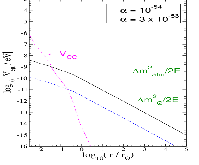
Figure 7: The MSW potential and the LR potential for a typical SN for two different $\alpha$ values that are allowed with the bounds obtained in this paper for $R_{LR}\ll R_{\rm gal}$. The SN model taken profile is a star with a mass of $15M_{\odot}$ and primordial metallicity equal to that of the Sun.

(i) The positions of the $H$ and $L$ resonances kuo , corresponding to $\Delta m^{2}_{\odot}$ and $\Delta m^{2}_{\rm atm}$ respectively, are shifted away from the center of the star by a factor of up to one order of magnitude.

(ii) If $V_{e\mu}$ dominates over $V_{cc}$ in the resonance region, the resonance is highly adiabatic, since the LR potential is in general smoother than the MSW potential. Therefore for larger $\alpha$ values, both the $H$ as well as $L$ resonances are adiabatic for practically all values of $\theta_{13}$. The SN neutrino spectra then lose the ability to reveal any information about $\theta_{13}$ in the absence of any shock wave effects. For example, no Earth matter effects earth-effects may be observed.

(iii) The shock fronts will reach the resonances at late times, $t>10$ s, when the neutrino flux has reduced a lot. As a result, the shock wave effects would be much harder to observe.

(iv) On the other hand, if any effects of non adiabaticity, e.g. Earth matter effects or shock wave effects, are identified in the neutrino spectra, the bound on $\alpha$ can be improved by almost an order of magnitude, to $\alpha\mathrel{\hbox to0.0pt{\lower 4.0pt\hbox{\hskip 1.0pt$\sim$}\hss}\raise 1.0pt\hbox{$<$}}10^{-54}$. Supernova neutrinos thus form the most sensitive probe for the LR forces, at least when their range is smaller than $R_{\rm gal}$.

(v) For $R_{LR}\mathrel{\hbox to0.0pt{\lower 4.0pt\hbox{\hskip 1.0pt$\sim$}\hss}\raise 1.0pt\hbox{$>$}}R_{\rm gal}$, the constraints obtained from the SN observation are expected to be comparable to those found from the solar neutrinos and KamLAND, since it is the approximate condition $(b~{}\alpha~{}M_{\rm gal}/R_{\rm gal})\ll\Delta m^{2}_{\rm solar}/(2E)$ that determines the allowed range of $\alpha$, like in Sec. V.

References

- (1) R. Foot, Mod. Phys. Lett. A 6, 527 (1991); X.-G. He, G. C. Joshi, H. Lew and R. R. Volkas, Phys. Rev D 43, 22 (1991).
- (2) M. Dine, W. Fischler and M. Srednicki, Phys. Lett. B 104, 199 (1981); J. E. Kim, Phys. Rev. Lett., 43 103 (1979).
- (3) Y. Chikashige, R. N. Mohapatra and R. D. Peccei, Phys. Lett. B 98, 265 (1981).
- (4) G. B. Gelmini and M. Roncadelli, Phys. Lett. B 99, 411 (1981).
- (5) L. J. Hall and S. J. Oliver, Nucl. Phys. Proc. Suppl. 137, 269 (2004) [arXiv:hep-ph/0409276] and references therein.
- (6) R. Fardon, A. E. Nelson and N. Weiner, JCAP 0410, 005 (2004) [arXiv:astro-ph/0309800]; M. Cirelli, M. C. Gonzalez-Garcia and C. Pena-Garay, Nucl. Phys. B 719, 219 (2005) [arXiv:hep-ph/0503028]; M. C. Gonzalez-Garcia, P. C. de Holanda, R. Zukanovich Funchal, Phys. Rev. D73 033008 (2006) [arXiv:hep-ph/0511093].
- (7) J. A. Grifols, E. Masso and S. Peris, Astropart. Phys. 2, 161 (1994); J. A. Grifols, E. Masso and R. Toldra, Phys. Lett. B 389, 563 (1996) [arXiv:hep-ph/9606377]; J. A. Grifols and E. Masso, Phys. Lett. B 579, 123 (2004) [arXiv:hep-ph/0311141].
- (8) A. S. Joshipura and S. Mohanty, Phys. Lett. B 584, 103 (2004) [arXiv:hep-ph/0310210].
- (9) R. N. Mohapatra et al., arXiv:hep-ph/0510213 and arXiv:hep-ph/0412099; M. S. Athar et al. [INO Collaboration], INO-2006-01, A Report of the INO Feasibility Study.
- (10) G. Dutta, A. S. Joshipura and K. B. Vijayakumar, Phys. Rev D 50, 2109 (1994).
- (11) E. Fischbach and C. L. Talmadge, The search for non-Newtonian gravity, New York, Springer Verlag (1999); E. G. Adelberger, B. R. Heckel, A. E. Nelson, arXive:hep-ph/0307284; B. R. Heckel et al., In Advances in Space Research, Proc. of 32nd COSPAR Scient. Assembly, Nagoya (1998); A. D. Dolgov, Phys. Rept. 320, 1 (1999).
- (12) J. G. Williams, S. G. Turyshev and D. H. Boggs, Phys. Rev. Lett. 93, 261101 (2004) [arXiv:gr-qc/0411113]; J. G. Williams, X. X. Newhall and J. O. Dickey, Phys. Rev. D 53, 6730 (1996); J. Muller et al., In ”Proc of 8th Marcel Grossman meeting on General Relativity, Jerusalem (1997).
- (13) M. Maltoni, T. Schwetz, M. A. Tortola and J. W. F. Valle, New J. Phys. 6, 122 (2004) [arXiv:hep-ph/0405172]; A. Strumia and F. Vissani, arXiv:hep-ph/0503246; G. L. Fogli, E. Lisi, A. Marrone, A. Palazzo and A. M. Rotunno, arXiv:hep-ph/0506307; A. Bandyopadhyay, S. Choubey, S. Goswami, S. T. Petcov and D. P. Roy, Phys. Lett. B 608, 115 (2005) [arXiv:hep-ph/0406328].
- (14) Neutrino Astrophysics, John N. Bahcall, Cambridge Univ. Press 1989.
- (15) A. D. Dolgov and G. G. Raffelt, Phys. Rev. D 52, 2581 (1995) [arXiv:hep-ph/9503438].
- (16) G. L. Fogli and E. Lisi, Astropart. Phys. 3, 185 (1995).
- (17) M. C. Gonzalez-Garcia, P. C. de Holanda, E. Masso and R. Zukanovich Funchal, arXiv:hep-ph/0609094.
- (18) A. S. Dighe and A. Yu. Smirnov, Phys. Rev. D 62, 033007 (2000) [arXiv:hep-ph/9907423]; A. Dighe, Nucl. Phys. Proc. Suppl. 143, 449 (2005) [arXiv:hep-ph/0409268].
- (19) R. C. Schirato and G. M. Fuller, astro-ph/0205390; R. Tomàs et al. JCAP 0409, 015 (2004) [arXiv:astro-ph/0407132]; G. L. Fogli, E. Lisi, A. Mirizzi and D. Montanino, JCAP 0504, 002 (2005) [arXiv:hep-ph/0412046]; B. Dasgupta and A. Dighe, arXiv:hep-ph/0510219.
- (20) H. Duan, G. M. Fuller and Y. Z. Qian, arXiv:astro-ph/0511275; H. Duan, G. M. Fuller, J. Carlson and Y. Z. Qian, arXiv:astro-ph/0606616; H. Duan, G. M. Fuller, J. Carlson and Y. Z. Qian, arXiv:astro-ph/0608050; S. Hannestad, G. G. Raffelt, G. Sigl and Y. Y. Y. Wong, arXiv:astro-ph/0608695.
- (21) S. E. Woosley, A. Heger and T. A. Weaver, Rev. Mod. Phys. 74, 1015 (2002).
- (22) T. K. Kuo and J. T. Pantaleone, Rev. Mod. Phys. 61, 937 (1989).
- (23) A. S. Dighe, M. T. Keil and G. G. Raffelt, JCAP 0306, 006 (2003) [arXiv:hep-ph/0304150]; A. S. Dighe, M. Kachelriess, G. G. Raffelt and R. Tomàs, JCAP 0401, 004 (2004) [arXiv:hep-ph/0311172].