Implications of measured properties
of the mixing matrix on mass matrices

Abstract

It is shown how the two experimentally measurable properties of the mixing matrix $V$, the asymmetry $\Delta(V)=|V_{12}|^{2}-|V_{21}|^{2}$ of $V$ with respect to the main diagonal and the Jarlskog invariant $J(V)={\rm Im}(V_{11}V_{12}^{*}V_{21}^{*}V_{22})$, can be exploited to obtain constraints on possible structures of mass matrices in the quark sector. Specific mass matrices are examined in detail as an illustration.

I Introduction

Flavor mixing in the quarks, in the Standard Model, arises from the unitary mixing matrices which diagonalize the corresponding mass matrices. In the quark sector 2 , in the physical basis, the CKM-mixing matrix is given by $V=V^{\dagger}_{\rm u}V_{\rm d}$, where the unitary matrices $V_{\rm u}$ and $V_{\rm d}$ diagonalize the up-quark and down-quark mass matrices, respectively. One can also work in a basis in which the up-quark (down-quark) mass matrix $M_{\rm u}$ ($M_{\rm d}$) is diagonal. In these bases the mixing matrix in the quark sector (like in the neutrino sector) will come from a single mass matrix. Clearly, if we knew the mass matrices fully then the corresponding mixing matrices are completely determined. In practice, the mass matrices are guessed at, while experiment can only determine the modulii of the matrix elements of the mixing matrix.

Recently it was shown 1 that a general property of the diagonalizing unitary matrix $U$ imply constraints on the corresponding hermitian mass matrix $M$. In particular, it was shown that the asymmetry $\Delta(U)$ w.r.t. the main diagonal and the Jarlskog invariant $J(U)$ 4 , which is a measure of CP-violation, can be directly expressed in terms of the eigenvalues $m_{i}$ and matrix elements $M_{ij}$ of the mass matrix $M$. Since $U^{\dagger}M\,U=\hat{M}={\rm diag}[m_{1},m_{2},m_{3}]$ one obtains

$$\Delta(U) \equiv |U_{12}|^{2}-|U_{21}|^{2}=|U_{23}|^{2}-|U_{32}|^{2}=|U_{31}|^{2}-|U_{13}|^{2}$$ (1)

$$= \frac{1}{D(m)}\{\sum_{k}\left(m_{k}~{}(M^{2})_{kk}-m_{k}^{2}~{}M_{kk}\right)\},$$

where

$$D(m)\equiv\begin{vmatrix}1&1&1\\ m_{1}&m_{2}&m_{3}\\ m_{1}^{2}&m_{2}^{2}&m_{3}^{2}\end{vmatrix}=(m_{2}-m_{1})(m_{3}-m_{1})(m_{3}-m_{2})$$ (2)

and

$$J(U)\equiv{\rm Im}(U_{11}U_{12}^{*}U_{21}^{*}U_{22})=\frac{{\rm Im}(M_{12}M_{23}M_{13}^{*})}{D(m)}.$$ (3)

Also, in terms of $M$ and its eigenvalues,

$$|U_{k\alpha}|^{2}=(N_{\alpha})_{kk},$$ (4)

where

$$N_{\alpha}=\frac{(m_{\beta}-M)(m_{\gamma}-M)}{(m_{\beta}-m_{\alpha})(m_{\gamma}-m_{\alpha})},~{}~{}~{}\alpha\neq\beta\neq\gamma,$$ (5)

with $\alpha$, $\beta$, $\gamma$ taking values from 1 to 3. Through this equation each $|U_{k\alpha}|$ can be calculated in terms of the eigenvalues (assuming non-degenerate eigenvalues which is true for the quarks) and matrix elements of $M$. Then, $|U_{k\alpha}|$ so calculated will automatically satisfy the unitarity relations $\sum_{k}|U_{k\alpha}|^{2}=1=\sum_{\alpha}|U_{\alpha k}|^{2}$. Thus, the calculated $\Delta(U)$ will be unique.

Eqns. $(\ref{7})$ and $(\ref{12})$ provide a simple criterion for selecting suitable mass matrices. In particular, the latter is remarkable in that it shows that if $M_{12}M_{23}M_{13}^{*}$ is real for a given $M$, then the Jarlskog invariant for the matrix $U$ which diagonalizes it vanishes.

II Choice for the mass matrix $\bm{M}$

We consider

$$M=\begin{pmatrix}0&a&d\\ a^{*}&0&b\\ d^{*}&b^{*}&c\end{pmatrix}.$$ (6)

For $d=0$ this reduces to the so called Fritzsch type mass matrix 7 ; 8 and will give $J(U)=0$. We now investigate its viability in both the up-quark and down-quark diagonal bases.

From the characteristic equation, we have

$$c = m_{1}+m_{2}+m_{3},$$ (7)

$$-(|a|^{2}+|b|^{2}+|d|^{2}) = m_{1}m_{2}+m_{1}m_{3}+m_{2}m_{3},$$ (8)

$$-c|a|^{2}+2{\rm Re}(abd^{*}) = m_{1}m_{2}m_{3}.$$ (9)

For the quark sector we need the mass hierarchy $|m_{1}|<<|m_{2}|<<|m_{3}|$. This coupled with Eqs. $(\ref{15})$ and $(\ref{16})$ require $m_{1},m_{3}>0$ and $m_{2}<0$, assuming $c>0$, for both up and down quarks. For simplicity we take $a$ and $b$ to be real and positive and $d$ as pure imaginary. Eq. $(\ref{16})$ then determines $a$. Eq. $(\ref{12})$ gives $ab|d|$. This together with Eq. $(\ref{15})$ fixes $b$ and $|d|$.

II.1 Down-quark diagonal basis

In this case $M=M_{\rm u}$ is the up-quark mass matrix which is diagonalized by $V_{\rm u}$. So the CKM-matrix $V=V^{\dagger}_{\rm u}$ since $V_{\rm d}=I$. Note that $\Delta(V_{\rm u})=-\Delta(V)$ and $J(V_{\rm u})=-J(V)<0$, so we choose $d=-i|d|$ in this case. For $J(V)$ and the quark masses we take the experimental values given in 3 : $J(V)=(3.08\pm 0.18)\times 10^{-5}>0$, $m_{\rm u}=(2.25\pm 0.75)\,{\rm Mev}$, $|m_{\rm c}|=(1.25\pm 0.09)\times 10^{3}\,{\rm Mev}$, and $m_{\rm t}=(174.2\pm 3.3)\times 10^{3}\,{\rm Mev}$. Using these we obtain $D(m)=(-3.83\pm 0.31)\times 10^{13}\,({\rm Mev})^{3}$ and

$$a = (53.5\pm 9.1)\,{\rm Mev},\quad b=(14.67\pm 0.55)\times 10^{3}\,{\rm Mev},$$

$$c = (17.30\pm 0.33)\times 10^{4}\,{\rm Mev},\quad|d|=(1.51\pm 0.27)\times 10^{3}\,{\rm Mev}.$$ (10)

Thus $M_{\rm u}$ is completely determined. We can calculate $\Delta(V)$ and individual $|V_{k\alpha}|^{2}$ using Eq. $(\ref{7})$ and Eq. $(\ref{5})$, respectively. The results for are given in columns Case A of Tables 1 and 2.

II.2 Up-quark diagonal basis

In this case $M=M_{\rm d}$ is the down-quark mass matrix which is diagonalized by $V_{\rm d}$. So the CKM-mixing matrix $V=V_{\rm d}$ since $V_{\rm u}=I$. Here $\Delta(V_{\rm d})=\Delta(V)$ and $J(V_{\rm d})=J(V)>0$, so we choose $d=i|d|$ in this case. For numerical analysis we take the values cited in 3 as inputs: $J(V)=(3.08\pm 0.18)\times 10^{-5}$, $m_{\rm d}=(5\pm 2)\,{\rm Mev}$, $|m_{\rm s}|=(95\pm 25)\,{\rm Mev}$, $m_{\rm b}=(4200\pm 70)\,{\rm Mev}$. These give $D(m)=(-1.80\pm 0.47)\times 10^{9}\,({\rm Mev})^{3}$ and

$$a = (22.0\pm 5.3)\,{\rm Mev},\quad b=(615\pm 86)\,{\rm Mev},$$

$$c = (4110\pm 74)\,{\rm Mev},\quad|d|=(4.10\pm 0.74)\,{\rm Mev}.$$ (11)

Using these we can calculate $\Delta(V)$ and individual $|V_{k\alpha}|^{2}$ as before. The results are given in columns Case B of Tables 1 and 2, respectively.

III Analisys of $\bm{\Delta(U)}$

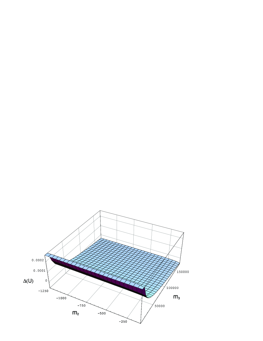
Figure 2: Behaviour of $\Delta(U)$ as a function of $m_{2}$ and $m_{3}$ for $m_{1}=3\,{\rm MeV}$. The intervals for $m_{2}$ and $m_{3}$ are the same as in Fig. 1. $\Delta(U)$ increases with the value of $m_{1}$. $\Delta(U)<0$ for the Case A corner (down–quark diagonal basis) where $|m_{2}|=m_{c}$ and $|m_{3}|=m_{t}$ and $\Delta(U)>0$ for the Case B corner (up–quark diagonal basis, $|m_{2}|=m_{s}$, $|m_{3}|=m_{b}$).

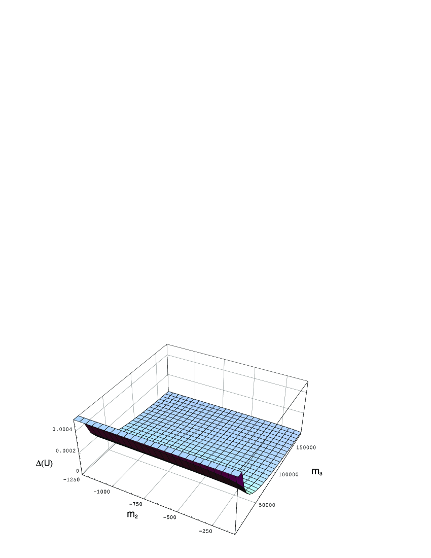
Figure 3: Behaviour of $\Delta(U)$ as a function of $m_{2}$ and $m_{3}$ for $m_{1}=7\,{\rm MeV}$. The intervals for $m_{2}$ and $m_{3}$ are the same as in Fig. 1. $\Delta(U)$ increases with the value of $m_{1}$ and now the whole graphic is positive.

We have also examined the dependence of $\Delta(U)$ as a function of $m_{2}$ and $m_{3}$ for three typical values of $m_{1}$ according to experimental $m_{\rm u}$ and $m_{\rm d}$ 3 . The results are displayed in Figures 1–3.

In general, we observe from Figs. 1–3 that the algebraic value of $\Delta(U)$ increases with the value of $m_{1}$ in the selected range of values of $m_{2}$ and $m_{3}$, from $-m_{\rm s}=-95\,{\rm MeV}$ to $-m_{\rm c}=-1.25\,{\rm GeV}$ and from $m_{\rm b}=4.20\,{\rm GeV}$ to $m_{\rm t}=174.2\,{\rm GeV}$, respectively. When $m_{1}=1.5\,{\rm MeV}$ (see Fig. 1) and also when $m_{1}=3\,{\rm MeV}$ (see Fig. 2), $\Delta(U)<0$ for the Case A corner (down–quark diagonal basis) where $|m_{2}|=m_{\rm c}$ and $|m_{3}|=m_{\rm t}$ and $\Delta(U)>0$ for the Case B corner (up–quark diagonal basis, $|m_{2}|=m_{\rm s}$, $|m_{3}|=m_{\rm b}$). For $m_{1}=7\,{\rm MeV}$, $\Delta(U)$ is positive for the whole graphic (see Fig. 3).

The increase in the algebraic value of $\Delta(U)$ with increasing $m_{1}$ (for given $|m_{2}|$ and $m_{3}$) observed in the graphs can be understood algebraically. For the given $M$, the condition $\Delta(U)>0$ can be expressed, in general, as

$$L<R$$ (12)

where

$$L\equiv m_{1}\,|m_{2}|\,c-m_{3}\,|a|^{2},$$ (13)

$$R\equiv m_{1}\,|b|^{2}-|m_{2}|\,|d|^{2}.$$ (14)

For the choice $a,b>0$ and $d=\mp i|d|$, Eq. (9) determines $a$, while Eq. (8) determines $b^{2}+|d|^{2}$ and $b|d|$ is given by Eq. (3) in terms of $J(U)$, $a$, and the masses. Thus, we can determine $b^{2}$ and $|d|^{2}$ individually. We assume $b>|d|$ as indicated by the numerical fits in both the cases. Since $m_{3}\gg|m_{2}|$ and $m_{1}$, an approximate expression for $L\approx-2m_{1}|m_{2}|^{2}$. Given the values of $m_{i}$, numerically $L_{\rm A}=-1.204\times 10^{7}\,({\rm MeV})^{3}$ and $L_{\rm B}=-8.055\times 10^{4}\,({\rm MeV})^{3}$.

For $R$ we obtain

$$2R = (m_{1}-|m_{2}|)(b^{2}+|d|^{2})+(m_{1}+|m_{2}|)(b^{2}-|d|^{2})$$

$$= (m_{1}-|m_{2}|)(b^{2}+|d|^{2})+(m_{1}+|m_{2}|)\sqrt{(b^{2}+|d|^{2})^{2}-(2b|d|)^{2}}.$$

Given the numerical values of the $m_{i}$, in either case, we can approximate this by expanding the square root to the first order to obtain

$$R\approx m_{1}(b^{2}+|d|^{2})-(m_{1}+|m_{2}|)\frac{b^{2}|d|^{2}}{b^{2}+|d|^{2}}.$$ (15)

For the given masses, $L$ can be neglected in comparison with the first term of $R$ since $b^{2}+|d|^{2}\approx|m_{2}|m_{3}$. Consequently, the condition Eq. (12) is effectively $R>0$. Since $b^{2}+|d|^{2}\approx|m_{2}|m_{3}$, this implies ($m_{1}\neq 0$)

$$\frac{m^{2}_{1}}{m^{2}_{3}}>J^{2}(U).$$ (16)

The approximate algebraic condition Eq. (16) gives an insight into the numerical trend that $\Delta(U)$ increases algebraically as $m_{1}$ increases.

IV Concluding Remarks

In this work we have examined constraints on mass matrices in the quark sector that arise due to measured properties of the mixing matrix. Working in a basis where down–quark (up–quark) mass matrix is diagonal and that the up–quark (down–quark) mass matrix has a specific texture, we reconstruct the moduli of the matrix elements of the mixing matrix taking the experimental values of the quark masses and the Jarlskog invariant as inputs. Comparing the modulii of the matrix elements of the mixing matrix thus reconstructed with the available data, we find better agreement for Case B when the down–quark mass matrix has the assumed form (see Eq. (6)) with the up–quark mass matrix diagonal rather than when the down-quark mass matrix is diagonal (Case A). This could well be attributed to the fact that the mass ratios in the two cases are very different. It is clear that in both cases one needs a more complicated mass matrix than the $M$ considered above.

Table 1: Experimental and predicted numerical values of the asymmetry $\Delta(V)$ (in units of $10^{-5}$). The calculated $\Delta(V)$ is exactly the same for $|V_{12}|^{2}-|V_{21}|^{2}$, etc. (see remark after Eq. (5)). $\overline{\Delta(V)}$ in row 4 is the average of the three values in rows 1 to 3. Case A: In down-quark diagonal basis, with experimental values 3 of up-quark masses and $J(V)$ as inputs. Case B: In up-quark diagonal basis, with experimental values 3 of down-quark masses and $J(V)$ as inputs.

Quantity	Experiment	Case A	Case B
$|V_{12}|^{2}-|V_{21}|^{2}$	$5\pm 64$	$6.2\pm 3.1$	$110\pm 40$
$|V_{23}|^{2}-|V_{32}|^{2}$	$5.1^{+1.3}_{-9.4}$	$6.2\pm 3.1$	$110\pm 40$
$|V_{31}|^{2}-|V_{13}|^{2}$	$5.05^{+0.53}_{-1.04}$	$6.2\pm 3.1$	$110\pm 40$
$\overline{\Delta(V)}$	$5^{+21}_{-22}$	$6.2\pm 3.1$	$110\pm 40$

Table 2: Experimental and predicted numerical values of the moduli of the matrix elements $|V_{ij}|$ of the CKM-matrix $V$. Case A: In down-quark diagonal basis, with experimental values 3 of up-quark masses and $J(V)$ as inputs. Case B: In up-quark diagonal basis, with experimental values 3 of down-quark masses and $J(V)$ as inputs.

Quantity	Experiment	Case A	Case B
$|V_{11}|$	$0.97383^{+0.00024}_{-0.00023}$	$0.9939\pm 0.0017$	$0.975\pm 0.012$
$|V_{12}|$	$0.2272^{+0.0010}_{-0.0010}$	$0.111\pm 0.015$	$0.224\pm 0.051$
$|V_{13}|$	$0.00396^{+0.00009}_{-0.00009}$	$0.00360\pm 0.00060$	$0.00123\pm 0.00013$
$|V_{21}|$	$0.2271^{+0.0010}_{-0.0010}$	$0.110\pm 0.015$	$0.221\pm 0.051$
$|V_{22}|$	$0.97296^{+0.00024}_{-0.00024}$	$0.9903\pm 0.0016$	$0.964\pm 0.010$
$|V_{23}|$	$0.04221^{+0.00010}_{-0.00080}$	$0.0843\pm 0.0031$	$0.145\pm 0.020$
$|V_{31}|$	$0.00814^{+0.00032}_{-0.00064}$	$0.0086\pm 0.0015$	$0.0331\pm 0.0060$
$|V_{32}|$	$0.04161^{+0.00012}_{-0.00078}$	$0.0839\pm 0.0031$	$0.141\pm 0.020$
$|V_{33}|$	$0.999100^{+0.000034}_{-0.000004}$	$0.99644\pm 0.00026$	$0.9895\pm 0.0029$

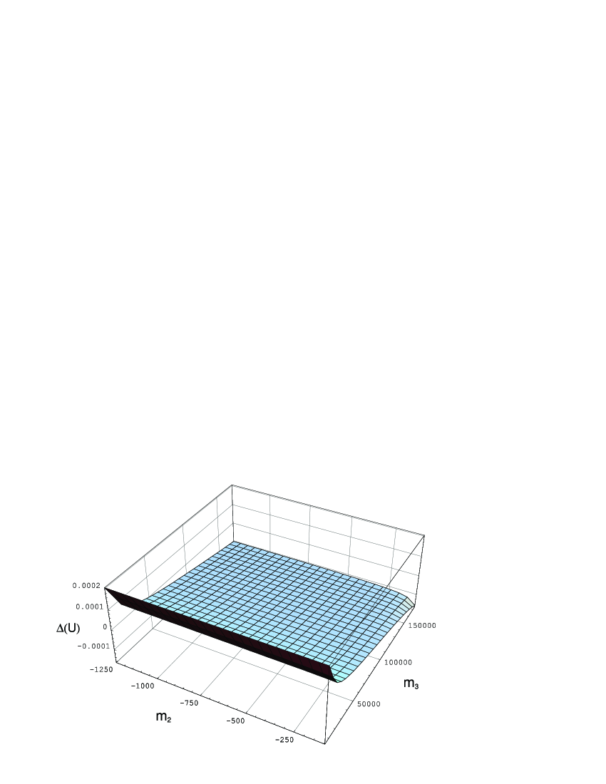
Figure 1: Behaviour of $\Delta(U)$ as a function of $m_{2}$ and $m_{3}$ for $m_{1}=1.5\,{\rm MeV}$. The range for $m_{2}$ is from $-m_{s}=-95\,{\rm MeV}$ to $-m_{c}=-1.25\,{\rm GeV}$ and for $m_{3}$ from $m_{b}=4.20\,{\rm GeV}$ to $m_{t}=174.2\,{\rm GeV}$. $\Delta(U)<0$ for the Case A corner (down–quark diagonal basis) where $|m_{2}|=m_{c}$ and $|m_{3}|=m_{t}$ and $\Delta(U)>0$ for the Case B corner (up–quark diagonal basis, $|m_{2}|=m_{s}$, $|m_{3}|=m_{b}$).

References

- (1) M. Kobayashi and T. Maskawa, Prog. Theor. Phys. D 35 (1973) 652; N. Cabibbo, Phys. Rev. Lett. 10 (1963) 531; L. L. Chau and W. -T. Keung, Phys. Rev. Lett. 53 (1984) 1802.
- (2) S. Chaturvedi and V. Gupta, Mod. Phys. Lett. A 21 (2006) 907.
- (3) C. Jarlskog, Phys. Rev. Lett. 55 (1985) 1039.
- (4) W. -M. Yao et al., J. Phys. G: Nucl. Part. Phys. 33 (2006) 1.
- (5) H. Fritzsch, Phys. Lett. B 70 (1977) 436, Phys. Lett. B 166 (1986) 423.
- (6) T. Kitazoe and K. Tanaka, Phys. Rev. 18 (1978) 3476; H. Georgi and D. Nanapoulos, Phys. Lett. B 82 (1979) 392; B. Stech, Phys. Lett. B 130 (1983) 189.