Can we probe right-handed charged quark currents?

Abstract

Different scenarios of new physics beyond the standard model give rise to a direct coupling of right-handed quarks to $W$ bosons. We will discuss how the prediction of the Callan-Treiman low energy theorem for the scalar $K\pi$ form factor in combination with recent data on $K^{L}_{\mu 3}$ decays can serve as a stringent test of the standard model (SM) and possible extensions, in particular right-handed charged quark currents (RHCs). In addition, we will comment on the impact of hadronic tau decay data on RHCs.

1 Introduction

Within the (not quite) decoupling low energy effective theory (LEET) scenario discussed by Jan Stern [1, 2], the only two operators appearing at NLO modify the charged current (CC) interaction. We will discuss whether it is possible to experimentally constrain the corresponding couplings. We will focus on the light quark sector where we will have to cope with the problem that it is not easy to disentangle the effects of non-standard electroweak couplings from (non-perturbative) QCD effects. We will see that in this respect $K^{L}_{\mu 3}$ decays present a stringent test of the SM and possible extensions giving rise to right-handed charged quark currents (RHCs).

In this talk we will consider a universal modification of the quark CC interaction leading to the following effective couplings at NLO for the vector and axial quark current, respectively:

$${\cal V}_{\mathit{eff}}^{ij} = (1+\delta)V_{L}^{ij}+\epsilon V_{R}^{ij}+\mathrm{NNLO}$$

$${\cal A}_{\mathit{eff}}^{ij} = -(1+\delta)V_{L}^{ij}+\epsilon V_{R}^{ij}+\mathrm{NNLO}~{},$$ (1)

where $V_{L}$ and $V_{R}$ are two a priori independent quark mixing matrices and the two parameters $\delta$ and $\epsilon$ measure the departure from the SM. The leptonic CC will not be modified [2]. Within the LEET scenario, the two parameters $\delta$ and $\epsilon$ can be related to the two NLO operators, but the same structure is shared by many models, as for example left-right symmetric extensions of the SM.

In tree level processes, we will encounter in the light quark sector, apart from $\delta$, the following two combinations:

$$\epsilon_{NS}=\epsilon\ \mathrm{Re}\Bigl{(}\frac{V_{R}^{ud}}{V_{L}^{ud}}\Bigr{)},\quad\epsilon_{S}=\epsilon\ \mathrm{Re}\Bigl{(}\frac{V_{R}^{us}}{V_{L}^{us}}\Bigr{)}~{}.$$ (2)

measuring the amount of $\bar{u}d$ and $\bar{u}s$ RHCs, respectively. We will in turn discuss the information we obtain on these parameters from $K^{L}_{\mu 3}$ and hadronic tau decays.

2 $K^{L}_{\mu 3}$ decays

The hadronic matrix element describing the $K^{0}_{\mu 3}$ decay can be written in terms of two form factors:

$$\langle\pi^{-}(p^{\prime})|\bar{s}\gamma_{\mu}u|K^{0}(p)\rangle=$$

$$(p^{\prime}+p)_{\mu}\ f^{K^{0}\pi^{-}}_{+}(t)+(p-p^{\prime})_{\mu}\ f_{-}^{K^{0}\pi^{-}}(t)~{},\qquad$$ (3)

where $t=(p^{\prime}-p)^{2}$. We will concentrate on the normalized scalar form factor

$$f(t)=\frac{f^{K^{0}\pi^{-}}_{+}(t)}{f^{K^{0}\pi^{-}}_{+}(0)}+\frac{t}{m^{2}_{K^{0}}-m^{2}_{\pi^{-}}}\frac{f^{K^{0}\pi^{-}}_{-}(t)}{f^{K^{0}\pi^{-}}_{+}(0)}$$ (4)

The Callan-Treiman low-energy theorem (CT) [3] fixes the value of $f(t)$ at the point $t=\Delta_{K\pi}=m_{K^{0}}^{2}-m_{\pi^{-}}^{2}$ in the $\mathrm{SU}(2)\times\mathrm{SU}(2)$ chiral limit. We can write

$$C=f(\Delta_{K\pi})=\frac{F_{K^{+}}}{F_{\pi^{+}}}\frac{1}{f_{+}^{K^{0}\pi^{-}}(0)}+\Delta_{CT},$$ (5)

where the CT discrepancy $\Delta_{CT}$ defined by Eq. (5) is expected to be small and eventually calculable in $\chi PT$. It is proportional to $m_{u}$ and/or $m_{d}$. In the limit $m_{d}=m_{u}$ at the NLO in $\chi PT$ one has for the CT discrepancy $\Delta_{CT}^{\mathrm{NLO}}=-3.5\times 10^{-3}$ [4]. We will focus the discussion on the neutral kaon mode since the analysis of the charged mode is subject to larger uncertainties related, in particular, to $\pi^{0}\eta$ mixing [5].

At low energies the form factor can be parameterized accurately in terms of only one parameter, $\ln C$, in a model independent way. To that end we employ a twice subtracted dispersion relation. One usually assumes that $f(t)$ has no zeros. In that case we can write [5]:

$$f(t)=\exp\Bigl{[}\frac{t}{\Delta_{K\pi}}(\ln C-G(t))\Bigr{]}~{},$$ (6)

where

$$G(t) = \frac{\Delta_{K\pi}(\Delta_{K\pi}-t)}{\pi}$$

$$\times\int_{t_{\pi K}}^{\infty}\frac{dx}{x}\frac{\phi(x)}{(x-\Delta_{K\pi})(x-t-i\epsilon)}~{}.$$

$t_{\pi K}$ is the threshold of $\pi K$ scattering and $\phi(t)$ is the phase of $f(t)$. At sufficiently low energies this phase should agree, due to Watson’s theorem, with the $s$-wave, $I=1/2,K\pi$ scattering phase, $\delta_{K\pi}(t)$. We take $\phi(t)=\delta_{K\pi}(t)$ up to an energy of $1.67~{}\mathrm{GeV}$. In this domain, as observed experimentally [6], the scattering amplitude is to a very good approximation elastic, and $\delta_{K\pi}$ is known precisely from a Roy-Steiner analysis [7]. Following Brodsky-Lepage [8], asymptotically the phase should reach $\pi$. In between the elastic and the asymptotic region we will assume $\phi(t)=\pi\pm\pi$. In principle it is possible to infer the phase of the form factor above the elastic region using a somewhat model dependent Omnes-Mushkelishvili construction as presented in Ref. [9]. In any case, due to the two subtractions the dispersive integral converges rapidly, keeping the error arising from the uncertainties in the high-energy behavior of the phase small. We nevertheless checked that in the low-energy region the phase of Ref. [9] reproduces our function $G(t)$ within errors. It can be observed that within the whole physical region the value of $G(t)$ stays at least a factor of five smaller than the expected value of $\ln C$ [5]. We include uncertainties on the extraction of $\delta_{K\pi}$ and the high-energy behavior into the error on $G(t)$.

Our dispersive representation allows to obtain the slope, $\lambda_{0}$, and the curvature, $\lambda^{\prime}$, of the form factor at $t=0$ in terms of only one parameter, $\ln C$:

$$\lambda_{0} = \frac{m_{\pi}^{2}}{\Delta_{K\pi}}(\ln C-G(0))~{},$$ (7)

$$\lambda^{\prime} = \lambda^{2}-2\frac{m_{\pi}^{4}}{\Delta_{K\pi}}G^{\prime}(0)~{},$$ (8)

where the Taylor expansion of the form factor has been written as follows: $f(t)=1+\lambda_{0}\frac{t}{m_{\pi}^{2}}+\frac{1}{2}\lambda^{\prime}(\frac{t}{m_{\pi}^{2}})^{2}+\ldots~{}.$ What is the value of $\ln C$? We can express $C$ in terms of the measured branching ratio Br $K^{+}_{l2}(\gamma)/\pi^{+}_{l2}(\gamma)$ [10], the inclusive decay rate $K^{L}_{e3}(\gamma)$  [11], and the value of $|{\cal V}_{\mathit{eff}}^{ud}|$ known from superallowed $0^{+}\to 0^{+}$ nuclear $\beta$-decays [12] as $C=B_{\mathit{exp}}\,r+\Delta_{CT}~{},$ with

$$B_{\mathit{exp}}=\Bigl{|}\frac{F_{K^{+}}{\cal A}_{\mathit{eff}}^{us}}{F_{\pi^{+}}{\cal A}_{\mathit{eff}}^{ud}}\Bigr{|}\frac{1}{|f_{+}^{K^{0}\pi^{-}}(0){\cal V}_{\mathit{eff}}^{us}|}|{\cal V}_{\mathit{eff}}^{ud}|$$

and

$$r=\Bigl{|}\frac{{\cal A}_{\mathit{eff}}^{ud}{\cal V}_{\mathit{eff}}^{us}}{{\cal V}_{\mathit{eff}}^{ud}{\cal A}_{\mathit{eff}}^{us}}\Bigr{|}~{}.$$

This gives to first order in $\epsilon$

$$\ln C = 0.2183\pm 0.0031+\tilde{\Delta}_{CT}+2(\epsilon_{S}-\epsilon_{NS})$$ (9)

$$= 0.2183\pm 0.0031+\Delta\epsilon$$

where $\tilde{\Delta}_{CT}=\Delta_{CT}/B_{\mathit{exp}}$. $\epsilon_{S}$ and $\epsilon_{NS}$ have been defined in Eq. (2).

Assuming SM weak interactions, i.e., $\epsilon_{S}=\epsilon_{NS}=0$, we obtain the following very precise prediction for $\lambda_{0}$ (cf. Eqs. (7),(9)):

$$\lambda_{0}=0.01524\pm 0.00044+0.0686\Delta_{CT}~{}.$$ (10)

This value can be compared with the slope parameter $\lambda_{\mathit{exp}}$ measured in $K^{L}_{\mu 3}$ decay experiments. It has to be stressed that the measured slope parameter cannot be directly interpreted as the slope of the form factor at $t=0$ since it is determined from a global fit to the measured decay distributions employing a linear parametrization, $f(t)=1+\lambda_{\mathit{exp}}t/m_{\pi}^{2}$, for the form factor. To better illustrate the problem, let us define an effective slope by $f(t)=1+\lambda_{\mathit{eff}}(t)\ t/m_{\pi}^{2}~{}.$ Since the curvature of the form factor is positive, $\lambda_{\mathit{eff}}(t)$ is a monotonically rising function of $t$. This means that $\lambda_{\mathit{exp}}\geq\lambda_{0}$, i.e., the measured slope parameter represents an upper bound for the value of $\lambda_{0}$.

Comparing the published value of the KTeV collaboration, $\lambda_{\mathit{exp}}=0.01372\pm 0.00131$ [13], and the preliminary value of NA48, $\lambda_{\mathit{exp}}=0.0120\pm 0.0017$ [14], with the SM prediction in Eq. (10), this indicates that we need a correction on the percent level, whereas estimates of the Callan-Treiman correction within $\chi PT$ give $\tilde{\Delta}_{CT}\sim 10^{-3}$ [4].

Thus, the Callan-Treiman low-energy theorem, in combination with measurements of the scalar $K\pi$ form factor offers a very interesting test of the SM and possible new physics.

If we admit that the charged current interaction gets modified and that we have RHCs, we get an additional correction sensitive to $\epsilon_{S}-\epsilon_{NS}$, cf. Eq. (9). $\epsilon_{S}$ and $\epsilon_{NS}$ represent the strengths of $\bar{u}d$ and $\bar{u}s$ RHCs, respectively. It should be mentioned on the one hand that RHCs can escape detection in $K^{L}_{\mu 3}$ decays, if the right-handed mixing matrix is aligned with the left-handed CKM matrix, i.e., $\epsilon_{S}=\epsilon_{NS}$. On the other hand, it is possible that $\epsilon_{S}$ gets enhanced by an inverse hierarchy of mixing matrix elements in the right-handed sector compared with the left-handed mixing matrix [1]. If we take the specific framework of the LEET [1], we expect from power counting arguments $\epsilon$ to be of the order of percent. Therefore $\epsilon_{NS}$ cannot be much larger than 0.01, whereas $\epsilon_{S}$ could be larger.

Let us now infer the value of $\Delta\epsilon$ from the data on $\lambda_{\mathit{exp}}$. Unfortunately the determination of $\ln C$ from $\lambda_{\mathit{exp}}$ is subject to large parametrization uncertainties. As explained above, the interpretation of $\lambda_{\mathit{exp}}$ in terms of the slope of the form factor is not clear and the measured slope parameter represents only an upper bound for $\lambda_{0}$. We therefore only get an upper bound for $\Delta\epsilon$:

$$\Delta\epsilon_{\mathit{max}} = -0.0178\pm 0.0156\pm 0.0040~{}[\mathrm{KTeV}]~{},$$

$$\Delta\epsilon_{\mathit{max}} = -0.0379\pm 0.0201\pm 0.0040~{}[\mathrm{NA48}]~{}.$$

The first error corresponds to the experimental error on $\lambda_{\mathit{exp}}$ and the branching ratios. The second one indicates the error on $G(t)$ inherent to our dispersive representation. The situation is illustrated for the KTeV data in Fig. 1 where we display the value of $\Delta\epsilon$ in terms of $\lambda_{\mathit{exp}}$. The upper hatched curve indicates the result choosing $\lambda_{\mathit{exp}}=\lambda_{\mathit{eff}}(0)$, the lower hatched curve $\lambda_{\mathit{exp}}=\lambda_{\mathit{eff}}(t_{0})$. Errors on the branching ratios and on $G(t)$ have been added in quadrature. The vertical lines indicate the KTeV measurement, whereas the horizontal line corresponds to the SM case with $\Delta\epsilon=\tilde{\Delta}_{CT}=\pm 0.0028$ [4]. Including the parametrization uncertainty as an error, we obtain $\Delta\epsilon=-0.03\pm 0.03$ (KTeV data) as indicated by the gray shaded area. The same procedure leads to $\Delta\epsilon=-0.05\pm 0.03$ using the preliminary NA48 data. These values are perfectly consistent with the expectation from the LEET, but pointing to an enhancement of $\epsilon_{S}$.

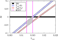
Figure 1: Impact of KTeV data on RHCs. Horizontal line: SM, $\Delta\epsilon=\tilde{\Delta}_{CT}=\pm~{}0.0028$, vertical lines: KTeV measurements of $\lambda_{0}$. Top hatched curve: $\lambda_{\mathit{exp}}=\lambda_{\mathit{eff}}(0)$ and bottom hatched curve: $\lambda_{\mathit{exp}}=\lambda_{\mathit{eff}}(t_{0})$ with uncertainties from branching ratios and from G(t) added in quadrature.

From the above discussion it is clear that the uncertainty due to the difficulties in interpreting the measured slope parameter dominates. The dispersive representation we proposed for the form factor [5], allows for an accurate description within the whole physical region in terms of only one parameter, $\ln C$. As explained above, a direct measurement of $\ln C$ can prove very important in testing the SM and possible physics beyond the SM. We discussed in which way a possible discrepancy between the SM, as indicated by Eq. (10), and the measured slope parameter, could be explained as an effect of RHCs.

3 Hadronic tau decays

The hadronic tau decays are semileptonic decays involving the charged current. Even though the different analyses of these decays done so far [15] have not yet reported any evidence of physics beyond the SM it seems interesting to reconsider them in the light of our generalization of the electroweak charged current.

For our analysis we have considered the normalized total hadronic width given by the ratio

$$R_{\tau,i}=\frac{\Gamma(\tau^{-}\to\nu_{\tau}\mathrm{hadrons}(\gamma))}{\Gamma(\tau^{-}\to\nu_{\tau}e^{-}\bar{\nu}_{e})}~{},$$ (11)

where $i$ can be $V,A$ or $S$ signifying that we are looking at the vector, axial or strange channel, respectively. Additional information is provided by spectral moments which explore the invariant mass distribution of final state hadrons [15].

The theoretical description of these ratios can be separated into several parts: the electroweak part, a perturbative QCD part and non-perturbative contributions, eventually calculable within the operator product expansion [16, 17]. The QCD corrections are functions of several QCD parameters: $\alpha_{s}$, quark masses and non-perturbative condensates.

Details of the analysis will be presented elsewhere [18]. Here we only want to summarize the main results. An important point is that present data only allow for putting constraints on the parameter $\epsilon_{NS}$ –in particular from the non-strange, $V+A$ channel– and the combination $\delta+\epsilon_{NS}$, showing up in the strange channel. In contrast to $\epsilon_{S}$, which can be enhanced if there is no strong Cabbibo suppression in the right-handed sector, we do not expect any enhancement for these two quantities. This means that we are looking for effects on the 1% level or even below. In fact, our knowledge of the QCD parameters entering the analysis has not yet reached a sufficient precision to determine effects of this order. Our conclusion is that presently the analysis of tau decay data does not exclude the presence of RHCs, in particular for the moment there is no evidence for an inconsistency with the expansion within the LEET, but on the other hand it does not allow for a quantitative determination of $\epsilon_{NS}$ and $\delta+\epsilon_{NS}$.

References

- [1] J. Stern, these proceedings.
- [2] J. Hirn and J. Stern, Eur. Phys. J. C 34 (2004) 447; J. Hirn and J. Stern, Phys. Rev. D 73 (2006) 056001.
- [3] R. F. Dashen and M. Weinstein, Phys. Rev. Lett. 22 (1969) 1337.
- [4] J. Gasser and H. Leutwyler, Nucl. Phys. B 250 (1985) 517.
- [5] V. Bernard, M. Oertel, E. Passemar and J. Stern, Phys. Lett. B 638 (2006) 480.
- [6] P. Estabrooks et al., Nucl. Phys. B 133 (1978) 490; D. Aston et al., Nucl. Phys. B 296 (1988) 493.
- [7] P. Buettiker, S. Descotes-Genon and B. Moussallam, Eur. Phys. J. C 33 (2004) 409.
- [8] G. P. Lepage and S. J. Brodsky, Phys. Lett. B 87 (1979) 359.
- [9] M. Jamin, J. A. Oller and A. Pich, Nucl. Phys. B 622 (2002) 279.
- [10] M. Jamin, J. A. Oller and A. Pich, arXiv:hep-ph/0605095.
- [11] T. Alexopoulos et al. [KTeV Collaboration], Phys. Rev. Lett. 93 (2004) 181802; F. Ambrosino et al. [KLOE Collaboration], Phys. Lett. B 632 (2006) 43; A. Lai et al. [NA48 Collaboration], Phys. Lett. B 602 (2004) 41.
- [12] W. J. Marciano and A. Sirlin, Phys. Rev. Lett. 96 (2006) 032002.
- [13] T. Alexopoulos et al. [KTeV Collaboration], Phys. Rev. D 70 (2004) 092007.
- [14] A. Winhart for the NA48 collaboration, talk given at HEP2005, Lisboa, Portugal.
- [15] M. Davier, A. Hocker and Z. Zhang, arXiv:hep-ph/0507078.
- [16] E. Braaten, S. Narison and A. Pich, Nucl. Phys. B 373 (1992) 581.
- [17] F. Le Diberder and A. Pich, Phys. Lett. B 289 (1992) 165.
- [18] V. Bernard, M. Oertel, E. Passemar, and J. Stern, in preparation.