The Need for Purely Laboratory-Based
Axion-Like Particle Searches

Abstract

The PVLAS signal has led to the proposal of many experiments searching for light bosons coupled to photons. The coupling strength probed by these near future searches is, however, far from the allowed region, if astrophysical bounds apply. But the environmental conditions for the production of axion-like particles in stars are very different from those present in laboratories. We consider the case in which the coupling and the mass of an axion-like particle depend on environmental conditions such as the temperature and matter density. This can relax astrophysical bounds by several orders of magnitude, just enough to allow for the PVLAS signal. This creates exciting possibilities for a detection in near future experiments.

I Introduction

Recently the PVLAS collaboration has reported the observation of a rotation of the polarization plane of a laser propagating through a transverse magnetic field Zavattini:2005tm . This signal could be explained by the existence of a new light neutral spin zero boson $\phi$, with a coupling to two photons Maiani:1986md ; Raffelt:1987im

$${\cal L}_{I}^{(-)}=\frac{1}{4M}\phi^{(-)}F_{\mu\nu}\widetilde{F}^{\mu\nu}\hskip 14.22636pt\textrm{or}\hskip 14.22636pt{\cal L}_{I}^{(+)}=\frac{1}{4M}\phi^{(+)}F_{\mu\nu}F^{\mu\nu}$$ (1)

depending on the parity of $\phi$, related to the sign of the rotation which up to now has not been reported. Such an Axion-Like Particle (ALP) would oscillate into photons and vice versa in the presence of an electromagnetic field in a similar fashion as the different neutrino flavors oscillate between themselves while propagating in vacuum.

The PVLAS signal, combined with the previous bounds from the absence of a signal in the BFRT collaboration experiment Cameron:1993mr , implies Zavattini:2005tm

$$1\ {\rm meV}\lesssim m\lesssim 1.5\ {\rm meV},\hskip 42.67912pt2\times 10^{5}\ {\rm GeV}\lesssim M\lesssim 6\times 10^{5}\ {\rm GeV},$$ (2)

with $m$ the mass of the new scalar.

It has been widely noticed that the interaction (1) with the strength (2) is in serious conflict with astrophysical constraints Raffelt:2005mt ; Ringwald:2005gf , while it is allowed by current laboratory and accelerator data Masso:1995tw ; Kleban:2005rj . This has motivated recent work on building models that evade the astrophysical constraints Masso:2005ym ; Jain:2005nh ; Jaeckel:2006id ; Masso:2006gc ; Mohapatra:2006pv , as well as alternative explanations to the ALP hypothesis Antoniadis:2006wp ; Gies:2006ca ; Abel:2006qt .

At the same time, many purely laboratory-based experiments have been proposed or are already on the way to check the particle interpretation of the PVLAS signal Ringwald:2003ns ; Rabadan:2005dm ; Pugnat:2005nk ; Gastaldi:2006fh ; Afanasev:2006cv ; Kotz:2006bw ; Cantatore:Patras ; BMV ; Chen:2003tp ; Gabrielli:2006im . It is important to notice, for the purpose of our paper, that these experiments are optical, and not high-energy, accelerator experiments.

Quite generally, these experiments will have enough sensitivity to check values of $M$ equal or greater than $10^{6}$ GeV, but, apart from Ref. Ringwald:2003ns , they do not have the impressive reach of the astrophysical considerations, implying $M\gtrsim 10^{10}$ GeV. Thus, if the PVLAS signal is due to effects other than $\phi-\gamma$ oscillations and the astrophysical bounds are applicable, these experiments can not detect any interesting signal.

However, the astrophysical bounds rely on the assumption that the vertex (1) applies under typical laboratory conditions as well as in the stellar plasmas that concern the astrophysical bounds. It is clear that, if one of the future dedicated laboratory experiments eventually sees a positive signal, this can not be the case.

In this work we investigate the simplest modification to the standard picture able to accommodate a positive signal in any of the forthcoming laboratory experiments looking for ALPs, namely that the structure of the interaction (1) remains the same in both environments, while the values of $M$ and $m$ can be different. Interestingly enough, the environmental conditions of stellar plasmas and of typical laboratory experiments are very different and thus one could expect a very big impact on $M$ and $m$.

We consider qualitatively the situation in which the dependence of $M$ and $m$ on the environmental parameters produces a suppression of ALP production in stellar plasmas. The main work of the paper is devoted to compute this suppression using a realistic solar model and to investigate how it relaxes the astrophysical bounds on the coupling (1). This leaves room for the proposed laboratory experiments to potentially discover such an axion-like particle.

In section II we revisit the astrophysical bounds and discuss general mechanisms to evade them. In the following section III, we present our scenario of environmental suppression and calculate the modified bounds. We present our conclusions and comment on the reach of proposed future laboratory experiments in section IV.

II Astrophysical Bounds and General Mechanisms to Evade them

Presuming the $\phi\gamma\gamma$ vertex (1), photons of stellar plasmas can convert into ALPs in the electromagnetic field of electrons, protons and heavy ions by the Primakoff effect, depicted schematically in Fig. 1. If $M$ is large enough, these particles escape from the star without further interactions constituting a non-standard energy-loss channel. This energy-loss channel accelerates the consumption of nuclear fuel and thus shortens the duration of the different stages of stellar evolution with respect to the standard evolution in which ALPs do not exist.

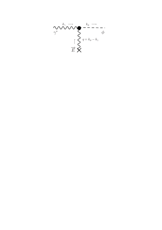
Figure 1: Primakoff processes in which a photon turns into an ALP in the electric field of a charged particle like a proton or electron.

In general, the astrophysical observations do agree with the theoretical predictions without additional energy-loss channels so one is able to put bounds on the interaction scale $M$ Raffelt:1996wa . The most important for our work are those coming from the lifetime of the Sun Frieman:1987ui , the duration of the red giant phase, and the population of Helium Burning (HB) stars in globular clusters Raffelt:1985nk ; Raffelt:1987yu . The last of them turns out to be the most stringent, implying

$$M>1.7\times 10^{10}\ \textrm{GeV}\equiv M_{\rm HB},$$ (3)

for $m<{\mathcal{O}}(1\ {\rm keV})$. Moreover, if ALPs are emitted from the Sun one may try to reconvert them to photons at Earth by the inverse Primakoff effect exploiting a strong magnetic field. This is the helioscope idea Sikivie:1983ip that it is already in its third generation of experiments. Recently, the CERN Axion Solar Telescope (CAST) collaboration has published their exclusion limits Zioutas:2004hi from the absence of a positive signal,

$$M>8.6\times 10^{9}\ \textrm{GeV}\equiv M_{\rm CAST},$$ (4)

for $m<0.02$ eV.

One should be aware that these astrophysical bounds rely on many assumptions to calculate the flux of ALPs produced in the plasma. In particular, it has been assumed widely in the literature that the same value of the coupling constant that describes $\phi-\gamma$ oscillations in a magnetic field in vacuum describes the Primakoff production in stellar plasmas, and the mass has been also assumed to be the same. We want to remark that this has been mainly an argument of pure simplicity. In fact, there are models in which $M$ depends on the momentum transfer $q$ at which the vertex is probed Masso:2005ym or on the effective mass $\omega_{P}$ of the plasma photons involved Masso:2006gc . These models have been built with the motivation of evading the astrophysical bounds on ALPs, by decreasing the effective value of the coupling $1/M$ in stellar plasmas in order to solve the inconsistency between the ALP interpretation of PVLAS and the astrophysical bounds. This has proven to be a very difficult task because of the extreme difference between the PVLAS value (2) and the HB (3) or CAST (4) exclusion limits. These models require very specific and somehow unattractive features like the presence of new confining forces or tuned cancellations (note, however, Abel:2006qt ). Anyway, they serve as examples of how $M$ (and eventually $m$) can depend on “environmental” parameters $\eta=q,\omega_{P}$, etc… (for other suitable parameters, see Table 1),

$$M\rightarrow M(\eta),\quad m\rightarrow m(\eta),$$ (5)

such that the production of ALPs is suppressed in the stellar environment.

Env. param.	Solar Core	HB Core	PVLAS
$T$ [keV]	$1.3$	$8.6$	$\sim 0$
$q^{2}$ [keV2]	$\sim 1$	$\sim 1$	$\sim 10^{-12}$
$\omega_{P}$ [keV]	$0.3$	$2$	$0$
$\rho$ [g cm-3]	$1.5\times 10^{2}$	$10^{4}$	$<10^{-5}$

Table 1: Comparison between the values of environmental parameters, such as the temperature $T$, typical momentum transfer $q$, plasma frequency $\omega_{P}$, and matter energy density $\rho$, in the stellar plasma and in the PVLAS experiment. Other parameters to consider could be the Debye screening scale $k_{s}$, or, to name something more exotic, the neutrino flux, or the average electromagnetic field.

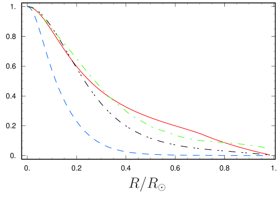
Figure 2: Environmental parameters as a function of the distance to the solar center. Temperature (solid, red), matter density (dashed, blue), Debye screening scale (double dashed, green) and plasma frequency (triple dashed, black), normalized to their values in the solar center, $T_{0}=1.35$ keV, $\rho_{0}=1.5\times 10^{2}$ g cm^-3, $k_{s0}=9$ keV, $\omega_{P0}=0.3$ keV for the solar model BS05(OP) of Bahcall et al. Bahcall:2004pz .

In the following, we will not try to construct micro-physical explanations for this dependence but rather write down simple effective models and fix their parameters in order to be consistent with the solar bounds and PVLAS or any of the proposed laboratory experiments.

A suppression of the production in a stellar plasma could be realized in two simple ways:

• either the coupling $1/M$ decreases (dynamical suppression) or

• $m$ increases to a value higher than the temperature such that the production is Boltzmann suppressed (kinematical suppression).

All the environmental parameters considered in this paper are much higher in the Sun than in laboratory conditions (see Table 1 and Fig. 2), so we shall consider $M(\eta)$ and $m(\eta)$ as monotonic increasing functions of $\eta$ with the values of $M(\sim 0)$ and $m(\sim 0)$ fixed by the laboratory experiments.

Clearly, both mechanisms are efficient at suppressing the production of ALPs in the Sun, but there is a crucial difference that results in some prejudice against mechanism (ii). Mechanism (i) works by making the already weak interaction between ALPs and the photons even weaker. The second mechanism, however, is in fact a strong interaction between the ALPs and ordinary matter, thereby making it difficult to implement without producing unwanted side effects. We will nevertheless include mechanism (ii) in our study, but one should always keep this caveat in mind.

As we said, $\eta$ in the stellar plasma is generally much higher than in laboratory-based experiments. It is then possible that new ALP physics produces also a big difference between the values of the ALP parameters, $m$ and $M$, in such different environments.

Let us remark on the a priori unknown shape of $M(\eta)$ and $m(\eta)$. In our calculations we use a simple step function (cf. Fig. 3), which has only one free parameter: the value for the environmental parameter where the production is switched off, $\eta_{\rm{crit}}$. In most situations this will give the strongest possible suppression. The scale $\eta_{\rm{crit}}$ can be associated with the scale of new physics responsible for the suppression. In what follows, we will consider only the effects of one environmental parameter at once although it is trivial to implement this framework for a set of parameters.

For simplicity, we restrict the study of the environmental suppression of ALPs to our Sun because we know it quantitatively much better than any other stellar environment. The group of Bahcall has specialized in the computation of detailed solar models which provide all the necessary ingredients to compute accurately the Primakoff emission. We have used the newest model, BS05(OP) Bahcall:2004pz , for all the calculations of this work (our accuracy goal is roughly $10\%$). The variation of some environmental parameters is displayed in Fig. 2 as a function of the distance from the solar center.

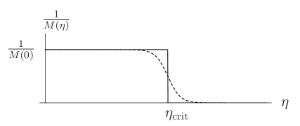
Figure 3: Coupling as a function of an environmental parameter $\eta$: The simple form used in our calculations (solid line) and a generic, more realistic, dependence (dashed).

III Numerical Results

Let us first state how a suppression $S$ of the flux of ALPs affects the bounds arising from energy loss considerations and helioscope experiments. If the flux of ALPs from a stellar plasma is suppressed by a factor $S$, the energy loss bounds on $M$ are relaxed by a factor of $\sqrt{S}$ while the CAST bound relaxes with $\sqrt[4]{S}$,

$$M_{\rm{loss}}\rightarrow\sqrt{S}\,M_{\rm{loss}}, \hskip 25.83325pt{\rm energy\ loss\ bound},$$ (6)

$$M_{\rm{CAST}}\rightarrow\sqrt[4]{S}\,M_{\rm{CAST}}, \hskip 25.83325pt{\rm{CAST\ bound}},$$ (7)

since the former depends only on the Primakoff production, $\sim 1/M^{2}$, and the latter gets an additional factor $\sim 1/M^{2}$ for the reconversion at Earth resulting in a total counting rate $\sim 1/M^{4}$.

III.1 Dynamical Suppression

We consider first a possible variation of the coupling that we have enumerated as mechanism (i). Treating the emission of ALPs as a small perturbation of the standard solar model, we can compute the emission of these particles from the unperturbed solar data. The $\gamma-\phi$ Primakoff transition amplitude can be written as (neglecting the plasma mass $\omega_{P}$ for the moment)

$$\Gamma(\omega)_{\gamma-\phi}=\frac{Tk^{2}_{s}}{64\pi}\int^{1}_{-1}d\cos\theta\frac{1+\cos\theta}{\kappa^{2}+1-\cos\theta}\frac{1}{M(\eta)^{2}},$$ (8)

where $\omega$ is the energy of the incoming photon, and

$$k^{2}_{s}=\frac{4\pi\alpha}{T}(n_{e}+\sum_{i}Z^{2}_{i}n_{i}),$$ (9)

is the Debye screening scale. $n_{i},Z_{i}$ are the number densities and charges of the different charged species of the plasma, $\alpha\simeq 1/137$, $n_{e}$ is the electron number density, $\cos\theta$ is the relative angle between the incoming photon and the outgoing ALP in the target frame (considered with infinite mass) and $\kappa^{2}=k_{s}^{2}/2\omega^{2}$. Integration over the whole Sun with the appropriate Bose-Einstein factors for the number density of photons gives the spectrum of ALPs (number of emitted ALPs per unit time per energy interval),

$$\frac{d^{2}N(\omega)}{d\omega dt}=4\pi\int_{0}^{R_{\odot}}R^{2}dR\frac{\omega^{2}}{\pi^{2}}\frac{\Gamma(\omega)_{\gamma-\phi}}{{\rm e}^{\omega/T}-1}\ \ \ .$$ (10)

(Remember that $T$, $k_{s}^{2}$, etc. depend implicitly on the distance $R$ from the solar center.)

As a check of our numerical computation we have computed the flux of standard ALPs at Earth which is shown in Fig. 4 and does agree with the CAST calculations Zioutas:2004hi .

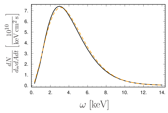
Figure 4: Our spectrum of ALPs at Earth (black solid) agrees reasonably well with that of the CAST collaboration Zioutas:2004hi (dashed orange) for $M=10^{10}\,\rm{GeV}$.

It is very important to differentiate two possibilities:

• $\eta$ is a macroscopic (averaged) environmental parameter given by the solar model and depending only on the distance $R$ from the solar center. Then the suppression acts as a step function in the $R$ integration (10) for the flux.

• $\eta$ depends on the microscopic aspects of the production like the momentum transfer $q^{2}$. Then the step function acts inside the integral in eq. (8).

We now start with the first possibility and let the second, which requires a different treatment, for subsubsection III.1.2.

III.1.1 Dynamical suppression from macroscopic environmental parameters

If $1/M(\eta)$ is a step function, ALP production is switched off wherever $\eta>\eta_{\rm crit}$. Let us call $R_{\rm crit}$ the radius at which the coupling turns off, i.e. $\eta(R_{\rm crit})=\eta_{\rm crit}$. Since the functions $\eta(r)$ shown in Fig. 2 are monotonous, we can calculate the suppression as a function of $R_{\rm crit}$ and then determine $\eta_{\rm crit}=\eta(R_{\rm crit})$.

We define the suppression efficiency, $S(\omega,R_{\rm crit})$, as the ratio of the flux of ALPs with energy $\omega$ with suppression, divided by the one without suppression,

$$S(\omega;R_{\rm crit})=\frac{d^{2}N(\omega;R_{\rm crit})}{d\omega\,dt}\left(\frac{d^{2}N(\omega)}{d\omega\,dt}\right)^{-1}.$$ (11)

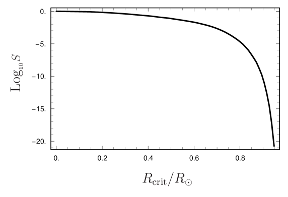
Figure 5: Suppression of the flux of ALPs $S(\omega_{0}=1\,\rm{keV},R_{\rm{crit}})$ as a function of $R_{\rm crit}$.

The CAST experiment is only sensitive to ALPs in the range of $(1-14)\,\rm{keV}$. Hence, we must suppress the production of ALPs only in this energy range. In order to provide a simple yet conservative bound we use the factor $S(\omega_{0},R_{\rm{crit}})$ evaluated at the energy $1\,\rm{keV}\leq\omega_{0}\leq 14\,\rm{keV}$ which maximizes $S$. We have checked that, in all cases of practical interest, $\omega_{0}$ is the CAST lower threshold, 1 keV. In Fig. 5, we plot $S(1\,{\rm keV},R_{\rm crit})$. In Tab. 2 we give some values for $S$ together with the corresponding values of $\eta_{\rm{crit}}$.

From the modified CAST bound (7),

$$M>\sqrt[4]{S(\omega_{0},R_{\rm crit})}\ 8.7\times 10^{9}\ \textrm{GeV},$$ (12)

we infer that in order to reconcile it with the PVLAS result, $M_{\rm PVLAS}\sim(10^{5}-10^{6})$ GeV, we need

$$S_{\rm CAST}\sim 10^{-20}\ \ \ .$$ (13)

Looking at Table 2, we find that this is possible, but the critical environmental parameters are quite small; for example, the critical plasma frequency is in the eV range. Moreover, the results are sensitive to the region close to the surface of the Sun where $\log(S)$ changes very fast and our calculation becomes somewhat less reliable.

$R_{\rm crit}/R_{\odot}$	$T_{\rm crit}\,[{\rm keV}]$	$\rho_{\rm crit}\,[{\rm g}\,{\rm cm}^{-3}]$	$\omega_{P,\rm{crit}}\,[{\rm keV}]$	$S$
$0$	$1.35$	$150$	$0.3$	$1$
$0.2$	$0.81$	$35$	$0.16$	$0.67$
$0.5$	$0.34$	$1.3$	$0.03$	$0.08$
$0.7$	$0.2$	$0.2$	$0.01$	$2\times 10^{-3}$
$0.8$	$0.12$	$0.09$	$0.008$	$2\times 10^{-5}$
$0.85$	$0.08$	$0.05$	$0.006$	$2\times 10^{-7}$
$0.9$	$0.05$	$0.03$	$0.004$	$4\times 10^{-11}$
$0.95$	$0.025$	0.009	0.0025	$\sim 10^{-20}$

Table 2: Several values of $S(\omega_{0}=1\,\rm{keV},R_{\rm{crit}})$ with their respective values of the suppression scales $\eta_{\rm crit}$.

We now take a look at the solar energy loss bound (6). The age of the Sun is known to be around $5.6$ billion years from radiological studies of radioactive crystals in the solar system (see the dedicated Appendix in Bahcall:1995bt ). Solar models are indeed built to reproduce this quantity (among others, like today’s solar luminosity, solar radius, etc…), so one might think that a model with ALP emission can be constructed as well to reproduce this lifetime. However, this seems not to be the case for large ALP luminosity Raffelt:1987yu and it is concluded that the exotic contribution cannot exceed the standard solar luminosity in photons. For our purposes this means

$$L_{\rm ALP}<L_{\odot}=3.846\times 10^{26}\ {\rm W}\sim 1.60\times 10^{30}\ {\rm eV}^{2},$$ (14)

with

$$L_{\rm ALP}\equiv\int_{0}^{\infty}d\omega\,\omega\,\frac{d^{2}N}{d\omega dt}.$$ (15)

We have computed the ALP emission in BS05(OP),

$$L_{\rm ALP}=1.8\times 10^{-3}\left(\frac{10^{10}\ \textrm{GeV}}{M}\right)^{2}L_{\odot}.$$ (16)

This value is slightly bigger than that of Ref. vanBibber:1988ge , which relies on an older solar model Bahcall:1981zh , probably as a consequence of the different data.

For the total flux, we find a suppression

$$\tilde{S}(R_{\rm{crit}})=\frac{L_{\rm{ALP}}(R_{\rm{crit}})}{L_{\rm{ALP}}},$$ (17)

which we plot in Fig. 6. Using the modified energy loss bound (6), (14) and (16) we get

$$M>\sqrt{\tilde{S}(R_{\rm{crit}})}\ 6\times 10^{9}\ \textrm{GeV},$$ (18)

and we need a much more moderate

$$\tilde{S}_{\rm{loss}}\sim 10^{-10}$$ (19)

to avoid a conflict between the PVLAS result and the energy loss argument. Accordingly, this bound alone requires values for the critical environmental parameters that are larger (and therefore less restrictive) than those from the CAST bound.

Figure 6: Suppression $\tilde{S}$ of the total flux of ALPs as a function of the critical radius $R_{\rm{crit}}$.

III.1.2 Dynamical suppression from microscopic parameters: $q^{2}$

In the previous subsection, we have considered macroscopic environmental parameters like, e.g., the temperature $T$. However, suppression could also result from a dependence on microscopic parameters like, e.g., the momentum transfer $q^{2}$ in a scattering event (not averaged).

In this section we discuss the well motivated (cf. Masso:2005ym ) example of a possible dependence $M=M(q^{2})$ on the momentum transfer involved in the Primakoff production (Fig. 1). Again, we use a step function to model the dependence on $q^{2}$,

$$\frac{1}{M(q^{2})}=\frac{1}{M(0)}\ \Theta(q^{2}_{\rm{crit}}-|q^{2}|)=\frac{1}{M(0)}\ \Theta(q^{2}_{\rm{crit}}-q_{m}^{2}-2k_{\phi}k_{\gamma}(1-\cos\theta)),$$ (20)

where $k_{\phi}$, $k_{\gamma}$ are the moduli of the momenta of the ALP and the photon. $q_{m}=|k_{\phi}-k_{\gamma}|$ is the smallest possible momentum transfer. Here, we will use the approximation $m=0$, but it will be crucial to take into account that photons have an effective mass

$$m^{2}_{\gamma}=\omega^{2}_{P}=\frac{4\pi\alpha n_{e}}{m_{e}},$$ (21)

so $q_{m}(\omega)=\omega-\sqrt{\omega^{2}-\omega_{P}^{2}}$. Note that the plasma mass is crucial because it ensures that $q_{m}>0$, i.e. it removes ALP production processes with very small momentum transfer which would be unsuppressed.

With this modification, Eq. (8) reads

$$\Gamma_{\gamma-\phi}(\omega)=\frac{Tk^{2}_{s}}{64\pi}\int_{-1}^{+1}d\cos\theta\frac{\sin^{2}\theta}{(x-\cos\theta)(y-\cos\theta)}\frac{1}{M^{2}(q^{2})}$$ (22)

with $x=(k_{\phi}^{2}+k_{\gamma}^{2})/2k_{\phi}k_{\gamma}$ and $y=x+k_{s}^{2}/2k_{\phi}k_{\gamma}$. The step function implies that only values of $\cos\theta$ satisfying

$$\cos\theta>1-\frac{q^{2}_{\rm{crit}}-q^{2}_{m}}{2\omega\sqrt{\omega^{2}-\omega^{2}_{P}}}$$ (23)

contribute to the integral. Hence, we find that the effect of the step function (20) is to restrict the integration limits of Eq. (22),

$$\Gamma_{\gamma-\phi}(\omega)=\frac{Tk_{s}^{2}}{64\pi M^{2}(0)}\int_{\delta(\omega)}^{+1}d\cos\theta\frac{\sin^{2}\theta}{(x-\cos\theta)(y-\cos\theta)},$$ (24)

with

$$\delta(\omega)=\left(\begin{array}[]{cccc}1&\textrm{for}&q_{\rm{crit}}<q_{m}(\omega)&\\ 1-\frac{q_{\rm{crit}}^{2}-q^{2}_{m}(\omega)}{2\omega\sqrt{\omega^{2}-\omega^{2}_{P}}}&\textrm{for}&q_{\rm{crit}}>q_{m}(\omega),&1-\frac{q_{\rm{crit}}^{2}-q^{2}_{m}(\omega)}{2\omega\sqrt{\omega^{2}-\omega^{2}_{P}}}>-1\\ -1&\textrm{for}&q_{\rm{crit}}>q_{m}(\omega),&1-\frac{q_{\rm{crit}}^{2}-q^{2}_{m}(\omega)}{2\omega\sqrt{\omega^{2}-\omega^{2}_{P}}}\leqslant-1\end{array}\right).$$ (25)

When $\delta(\omega)=1$, the integral is zero and Primakoff conversion is completely suppressed. This happens for values of the plasma frequency $\omega_{P}$ and the energy $\omega$ for which the minimum momentum transfer is already larger than the cut-off scale $q_{\rm{crit}}$. We point out that this is an energy dependent statement. For $\omega\gg\omega_{P}$ large enough, $q_{m}$ is small enough to satisfy $q_{\rm{crit}}\gg q_{m}$. When this is the case we have only partial suppression. The integral goes only over the small interval $[\delta(\omega),1]$ where $\delta(\omega)\approx 1-q_{\rm{crit}}^{2}/2\omega^{2}$, $x\approx 1$ and $y\approx 1+k_{s}^{2}/2\omega^{2}$. Then the integral can be easily estimated by the value of the integrand at $\cos\theta=1$,

$$\Gamma_{\gamma-\phi}(\omega)\sim\frac{Tk_{s}^{2}}{64\pi M^{2}}\frac{4\omega^{2}}{k_{s}^{2}}\frac{q_{\rm{crit}}^{2}}{2\omega^{2}},\quad\quad\quad{\rm{for}}\,\,\omega\gg\omega_{P},\,k_{s},\,q_{\rm{crit}}.$$ (26)

Notice that although we have used the strongest possible suppression, a step function, at the end of the day, at high energies, the transition rate is only suppressed by a factor $q_{\rm{crit}}^{2}/k_{s}^{2}$. This means that the $\gamma^{*}-\phi$ transition is suppressed at most quadratically.

This holds even for a generic suppressing factor $F(q^{2})=M(q^{2})/M(0)$. The limitation comes from the part of the integral which is close to $\cos\theta=1$. There the integrand is a constant, $1+\cos\theta/(y-1)\sim 4\omega^{2}/k_{s}^{2}$. By continuity, the suppression factor $F(q^{2})$, whatever it is, must be close to unity because $q^{2}$ is very close to zero and normalization requires $F(q^{2}=0)=1$. This holds for values of $q^{2}$ up to a certain range, limited by the shape of $F(q^{2})$. Defining $q_{\rm{crit}}^{2}$ as the size of the interval where $F(|q^{2}|\lesssim q_{\rm{crit}}^{2})\sim 1$, then $q_{\rm{crit}}^{2}=|q^{2}|$ gives a minimum value for $\cos\theta$ for which the integrand is nearly constant ($\cos\theta_{m}\sim 1-q_{\rm{crit}}^{2}/2\omega^{2}$), leading to

$$\Gamma(\omega)\propto\int^{1}_{-1}d\cos\theta\,\frac{1+\cos\theta}{y-\cos\theta}\,F(q^{2})\gtrsim\int^{1}_{\cos\theta_{m}}d\cos\theta\,\frac{4\omega^{2}}{k_{s}^{2}}\sim\frac{2q_{\rm{crit}}^{2}}{k_{s}^{2}}.$$ (27)

Proceeding along the lines of the previous section we can calculate the suppression factors for the CAST experiment $S$ and the corresponding $\tilde{S}$ that appears in the energy loss considerations. The results are plotted in Fig. 7.

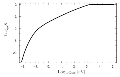
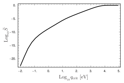
Figure 7: Suppression factor $S$ for CAST, and $\tilde{S}$ for the energy loss arguments as a function of $q_{\rm{crit}}$.

Using the required suppression (13), $S\sim 10^{-20}$, for CAST and (19), $\tilde{S}\sim 10^{-10}$, for the energy loss arguments, we infer that sufficient suppression requires

$$q_{\rm{crit}}\lesssim 10^{-2}\,\rm{eV}.$$ (28)

Although this seems rather small it is nevertheless quite big compared to the typical momentum transfer in the PVLAS experiment,

$$q_{\rm{PVLAS}}\approx\frac{m^{2}_{\phi}}{2\omega}\sim 6\times 10^{-7}\,\rm{eV}.$$ (29)

III.2 Kinematical Suppression

So far, we have suppressed the production of ALPs by reducing their coupling to photons. Now, we consider the possibility that the suppression originates from an increase of the ALP’s effective mass. Clearly, if the latter is larger than the temperature, only the Boltzmann tail of photons with energies higher than the mass can contribute to ALP production.

If we consider macroscopic environmental parameters $\eta(R)$ and, again, assume the simplest dependence on these parameters,

$$m(\eta<\eta_{\rm{crit}})=m\ \ (\sim\textrm{meV}),\hskip 28.45274ptm(\eta>\eta_{\rm{crit}})=\infty,$$ (30)

the suppression is identical to the one computed in Sect. III.1.1, since the Boltzmann tail vanishes for infinite mass. Accordingly, Figs. 5 and 6 give the correct suppression also for the case of an environment dependent mass.

Before we continue let us point out that a strong dependence of the mass on environmental parameters such as in Eq. (30) is problematic because it requires a strong coupling between the ALP and its environment. This still holds even if we require only $m(\eta>\eta_{crit})\gtrsim 10\,\rm{keV}$. The strong coupling is likely to lead to unwanted side effects, as we commented in Sec. II, but let us however discuss some phenomenological aspects which could distinguish kinematical suppression from a dynamical suppression via the coupling. As an explicit example, we discuss a dependence on the density $\rho$. The wave equation for the ALP will be

$$\Box\phi+m^{2}(\rho(x))\phi=0.$$ (31)

The effective mass, $m(\rho(x))$, acts as a potential for $\phi$. This can actually lead to a new way to avoid the CAST bound. For example consider a situation where ALPs are emitted with energy $\omega$. When they encounter a macroscopic “wall” with $m(\rho_{\rm{wall}})>\omega$ on their way to the CAST detector, they will be reflected due to energy conservation (tunneling through a macroscopic barrier is negligible). In other words, they will not be able to reach the CAST detector and can not be observed. In this case only the energy loss arguments require a suppression of the production (19) whereas the stronger constraint (13) from CAST is circumvented by the reflection.

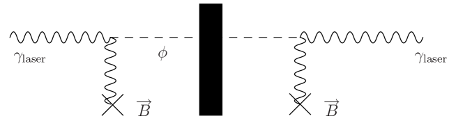
Figure 8: Schematic view of a “light shining through a wall” experiment. (Pseudo-)scalar production through photon conversion in a magnetic field (left), subsequent travel through an (opaque) wall, and final detection through photon regeneration (right).

This effect will also play a central role in the interpretation of the PVLAS result in terms of an ALP. Note that the interaction region (length $L$) of the PVLAS set up is located inside a Fabri-Perot cavity which enlarges the optical path of the light inside the magnetic field by a factor $N_{r}\sim 10^{5}$ accounting for the number of reflections inside the cavity.. In the standard ALP scenario, the ALPs created along one path cross the mirror and escape from the cavity. Coherent production takes place only over the length $L$. The net result produces a rotation non-linear in $L$ but only linear in $N_{r}$ Raffelt:1987im ,

$$|\Delta\theta|=N_{r}\left(\frac{B\omega}{Mm^{2}}\right)^{2}\sin^{2}\left(\frac{Lm^{2}}{4\omega}\right).$$ (32)

However, if $m=m(\rho)$ the ALPs have a potential barrier in this mirror and they will be reflected in the same way as the photons. In fact, the whole setup now acts like one pass through an interaction region of length $N_{r}L$. The ALP field in the cavity will increase now non-linearly in $N_{r}L$ modifying the predicted rotation in the following way

$$|\Delta\theta_{\rm modified}|=\left(\frac{B\omega}{Mm^{2}}\right)^{2}\sin^{2}\left(\frac{N_{r}Lm^{2}}{4\omega}\right),$$ (33)

where $\omega$ is the frequency of the laser. For small enough $m\lesssim{\rm few}\times 10^{-6}\,\rm{eV}$ this grows as

$$|\Delta\theta_{\rm modified}|\approx\frac{N^{2}_{r}L^{2}B^{2}}{16M^{2}}.$$ (34)

Under these conditions the PVLAS experiment cannot fix $m$ using the exclusion bounds from BFRT. Using Eq. (33) the rotation measurement suggests, however, a much more interesting value

$$M_{\rm modified}\sim 10^{8}\ {\rm GeV},\quad{\rm{for}}\quad m\lesssim{\rm few}\times 10^{-6}{\rm{eV}},$$ (35)

where we have used $l\sim 1$ m, $N_{r}\sim 10^{5}$ and $\omega\sim 1$ eV for the PVLAS setup. That could be reconciled more easily with astrophysical bounds within our framework.

Such an effective mass will also play a role in “light shining through a wall” experiments (cf. Fig. 8). Typically, the wall in such an experiment will be denser than the critical density $\rho_{\rm{crit}}$ required from the energy loss argument. Consequently, an ALP produced on the production side of such an experiment will be reflected on the wall and cannot be reconverted in the detection region. Hence, such an experiment would observe nothing if a density dependent kinematical suppression is realized in nature.

IV Summary and conclusions

The PVLAS collaboration has reported a non-vanishing rotation of the polarization of a laser beam propagating through a magnetic field. The most common explanation for such a signal would be the existence of a light (pseudo-)scalar axion-like particle (ALP) coupled to two photons. However, the coupling strength required by PVLAS exceeds astrophysical constraints by many orders of magnitude. In this paper, we have quantitatively discussed ways to evade the astrophysical bounds by suppressing the production of ALPs in astrophysical environments, in particular in the Sun.

The simplest way to suppress ALP production is to make the coupling $1/M$ of ALPs to photons small in the stellar environment. Motivated by microphysical models Masso:2005ym ; Masso:2006gc ; Abel:2006qt ; Mohapatra:2006pv , we considered a dependence of $M$ on environmental parameters, such as temperature, plasma mass $\omega_{P}$, or density $\rho$. One of our main results is that it is not sufficient to suppress production in the center of the Sun only. One has to achieve efficient suppression also over a significant part of the more outer layers of the Sun. As apparent from Tables 1, 2 and Eq. (13), it is possible to reconcile the PVLAS result with the bound from the CERN Axion Solar Telescope (CAST) if strong suppression sets in at sufficiently low critical values of the environmental parameters, e.g. $\rho\sim 10^{-3}$ g/cm³, or $\omega_{P}\sim$ eV. The bounds arising from solar energy loss considerations are less restrictive (cf. Eq. (19) and Figs. 2, 6). As an alternative suppression mechanism, we have also exploited an effective mass that grows large in the solar environment. This case, too, requires that the effect sets in already for low critical values of the environmental parameters (cf. Figs. 5, 6).

Most proposed near-future experiments to test the PVLAS ALP interpretation are of the “light shining through a wall” type (cf. Fig. 8). In these experiments, the environment, i.e. the conditions in the production and regeneration regions, may be modified. The above mentioned critical values are small enough that they may be probed in such modifications. For example, a density dependence may be tested by filling in buffer gas.

In conclusion, the PVLAS signal has renewed the interest in light bosons coupled to photons. The astrophysical bounds, although robust, are model-dependent and may be relaxed by many orders of magnitude. Therefore, the upcoming laboratory experiments are very welcome and may well lead to exciting discoveries in a range which was thought to be excluded.

V acknowledgments

Two of us (EM and JR) acknowledge support by the projects FPA2005-05904 (CICYT) and 2005SGR00916 (DURSI).

References

- (1) E. Zavattini et al. [PVLAS Collaboration], Phys. Rev. Lett. 96, 110406 (2006) [hep-ex/0507107].
- (2) L. Maiani, R. Petronzio and E. Zavattini, Phys. Lett. B 175, 359 (1986).
- (3) G. Raffelt and L. Stodolsky, Phys. Rev. D 37, 1237 (1988).
- (4) U. Gastaldi, on behalf of the PVLAS Collaboration, talk at ICHEP‘06, Moscow, http://ichep06.jinr.ru/reports/42_1s2_13p10_gastaldi.ppt
- (5) R. Cameron et al. [BFRT Collaboration], Phys. Rev. D 47, 3707 (1993).
- (6) G. G. Raffelt, [hep-ph/0504152].
- (7) A. Ringwald, J. Phys. Conf. Ser. 39, 197 (2006) [hep-ph/0511184].
- (8) E. Masso and R. Toldra, Phys. Rev. D 52, 1755 (1995) [hep-ph/9503293].
- (9) M. Kleban and R. Rabadan, [hep-ph/0510183].
- (10) E. Masso and J. Redondo, JCAP 0509, 015 (2005) [hep-ph/0504202].
- (11) P. Jain and S. Mandal, [astro-ph/0512155].
- (12) J. Jaeckel, E. Masso, J. Redondo, A. Ringwald and F. Takahashi, [hep-ph/0605313].
- (13) E. Masso and J. Redondo, Phys. Rev. Lett. 97, 151802 (2006), [hep-ph/0606163].
- (14) R. N. Mohapatra and S. Nasri, [hep-ph/0610068].
- (15) I. Antoniadis, A. Boyarsky and O. Ruchayskiy, [hep-ph/0606306].
- (16) H. Gies, J. Jaeckel and A. Ringwald, Phys. Rev. Lett. 97, 140402 (2006) [hep-ph/0607118].
- (17) S. A. Abel, J. Jaeckel, V. V. Khoze and A. Ringwald, [hep-ph/0608248].
- (18) A. Ringwald, Phys. Lett. B 569, 51 (2003) [hep-ph/0306106].
- (19) P. Pugnat et al., Czech. J. Phys. 55, A389 (2005); Czech. J. Phys. 56, C193 (2006).
- (20) R. Rabadan, A. Ringwald and K. Sigurdson, Phys. Rev. Lett. 96, 110407 (2006) [hep-ph/0511103].
- (21) U. Gastaldi, [hep-ex/0605072].
- (22) A. V. Afanasev, O. K. Baker and K. W. McFarlane [LIPSS Collaboration], [hep-ph/0605250].
- (23) U. Kötz, A. Ringwald and T. Tschentscher [APFEL Collaboration], [hep-ex/0606058]; K. Ehret et al. [ALPS Collaboration], in preparation.
- (24) G. Cantatore [PVLAS Collabortion], “Probing the quantum vacuum with polarized light: a low energy photon-photon collider at PVLAS,” 2nd ILIAS-CERN-CAST Axion Academic Training 2006, http://cast.mppmu.mpg.de/
- (25) C. Rizzo [BMV Collaboration], “Laboratory and Astrophysical Tests of Vacuum Magnetism: the BMV Project,” 2nd ILIAS-CAST-CERN Axion Training, May, 2006, http://cast.mppmu.mpg.de/
- (26) S. J. Chen et al. [Q & A Collaboration], [hep-ex/0308071].
- (27) E. Gabrielli, K. Huitu and S. Roy, [hep-ph/0604143].
- (28) For a complete description see: G. G. Raffelt, Stars as laboratories for fundamental physics”, Chicago Univ. Press. (1996)
- (29) J. A. Frieman, S. Dimopoulos and M. S. Turner, Phys. Rev. D 36, 2201 (1987).
- (30) G. G. Raffelt, Phys. Rev. D 33, 897 (1986).
- (31) G. G. Raffelt and D. S. P. Dearborn, Phys. Rev. D 36, 2211 (1987).
- (32) P. Sikivie, Phys. Rev. Lett. 51, 1415 (1983) [Erratum-ibid. 52, 695 (1984)].
- (33) K. Zioutas et al. [CAST Collaboration], Phys. Rev. Lett. 94, 121301 (2005) [hep-ex/0411033].
- (34) J. N. Bahcall, A. M. Serenelli and S. Basu, Astrophys. J. 621, L85 (2005) [astro-ph/0412440].
- (35) J. N. Bahcall and M. H. Pinsonneault, Rev. Mod. Phys. 67, 781 (1995) [hep-ph/9505425].
- (36) K. van Bibber, P. M. McIntyre, D. E. Morris and G. G. Raffelt, Phys. Rev. D 39, 2089 (1989).
- (37) J. N. Bahcall, W. F. Huebner, S. H. Lubow, P. D. Parker and R. K. Ulrich, Rev. Mod. Phys. 54, 767 (1982).