The mass hierarchy with atmospheric neutrinos at INO

Abstract

We study the neutrino mass hierarchy at the magnetized Iron CALorimeter (ICAL) detector at India-based Neutrino Observatory with atmospheric neutrino events generated by the Monte Carlo event generator Nuance. We judicially choose the observables so that the possible systematic uncertainties can be reduced. The resolution as a function of both energy and zenith angle simultaneously is obtained for neutrinos and anti-neutrinos separately from thousand years un-oscillated atmospheric neutrino events at ICAL to migrate number of events from neutrino energy and zenith angle bins to muon energy and zenith angle bins. The resonance ranges in terms of directly measurable quantities like muon energy and zenith angle are found using this resolution function at different input values of $\theta_{13}$. Then, the marginalized $\chi^{2}$s are studied for different input values of $\theta_{13}$ with its resonance ranges taking input data in muon energy and zenith angle bins. Finally, we find that the mass hierarchy can be explored up to a lower value of $\theta_{13}\approx 5^{\circ}$ with confidence level $>$ 95% in this set up.

I introduction

The recent experiments reveal that neutrinos have mass and they oscillate pdg from one flavor to another flavor as they travel. In the standard framework of oscillation scenario with three active neutrinos, the mass eigenstates $|\nu_{i}\rangle$ and the flavor eigen states $|\nu_{\alpha}\rangle$ are related by a mixing matrix $U$ pmns :

$$|\nu_{\alpha}\rangle=U_{\alpha i}|\nu_{i}\rangle.$$ (1)

The flavor mixing matrix in vacuum $U$ (PDG representation pdg ) is

$$\left(\begin{array}[]{c c c}c_{12}c_{13}&s_{12}c_{13}&s_{13}e^{-i\delta}\\ -s_{12}c_{23}-c_{12}s_{23}s_{13}e^{i\delta}&c_{12}c_{23}-s_{12}s_{23}s_{13}e^{i\delta}&s_{23}c_{13}\\ s_{12}s_{23}-c_{12}c_{23}s_{13}e^{i\delta}&-c_{12}s_{23}-s_{12}c_{23}s_{13}e^{i\delta}&c_{23}c_{13}\end{array}\right).$$ (5)

In this oscillation picture, there are six parameters: two mass squared differences $\Delta m_{ij}^{2}$ ($\Delta m_{12}^{2},\Delta m_{32}^{2}$), three mixing angles ($\theta_{12},\theta_{23},\theta_{13}$), and a CP-violating phase $\delta$. At present, information is available on two neutrino mass-squared differences and two mixing angles: from atmospheric neutrinos one gets the best-fit values with $3\sigma$ error $|\Delta m^{2}_{32}|\simeq 2.50^{+.52}_{-0.60}\times 10^{-3}$ eV², $\theta_{23}\simeq$ ${45.0^{\circ}}^{+10.55^{\circ}}_{-9.44^{\circ}}$; while solar neutrinos tell us $\Delta m^{2}_{21}\simeq 7.9\times 10^{-5}$ eV², $\theta_{12}\simeq{33.21^{\circ}}^{+6.02^{\circ}}_{-3.88^{\circ}}$ Schwetz:2006dh . Here $\Delta m^{2}_{ij}$= $m^{2}_{i}-m^{2}_{j}$. The present experiments are sensitive to $\left|\Delta m_{32}^{2}\right|$ only and the both sign of $\Delta m_{32}^{2}$ fit the data equally well.

The neutrino mass hierarchy, whether normal ($m_{3}^{2}>m_{2}^{2}$), or inverted ($m_{2}^{2}>m_{3}^{2}$), is of great theoretical interest. For example, the grand unified theory favors normal hierarchy. It can be qualitatively understood from the fact that it relates leptons to quarks and quark mass hierarchies are normal. The inverted mass hierarchy which is unquarklike, would probably indicate a global leptonic symmetryMohapatra:2004vr .

For nonzero value of $\theta_{13}$, the hierarchy can be determined from the matter effect on neutrino oscillation. The contributions of this effect to the effective Lagrangian during the propagation through matter are opposite for neutrino and anti-neutrino, which depends mainly on the value of $\theta_{13}$ and the sign of $\Delta m_{32}^{2}$. So the total number of observed events is expected to differ for normal hierarchy (NH) and inverted hierarchy (IH). The hierarchy can be more prominently distinguished if the experiment is able to count neutrinos and anti-neutrinos separately. This needs charge identification of the produced leptons.

In case of $\theta_{13}=0$, the mass hierarchy can also be observable in principle even in case of vacuum oscillation due to nonzero value of $\Delta m_{21}^{2}$deGouvea:2005hk .

Presently over the world, there are many ongoing and planned experiments: MINOSZois:2004ns , T2KYamada:2006hi , ICARUSKisiel:2005ti , NOVARay:2006ke , D-CHOOZHorton-Smith:2006yh , UNOJung:1999jq , SKIIIBack:2004qi , OPERADiCapua:2005bd , Hyper-KNakamura:2003hk , and many others. It is notable that all these experiments are planned in the north hemisphere of the Earth. Among them MINOS is the only magnetized one and has a good charge identification capability. A large magnetized ICAL detector is under strong consideration for the proposed India-based Neutrino Observatory (INO)ino near the equator. Since it has high charge identification capability $(\mathrel{\hbox to0.0pt{\raise 2.15277pt\hbox{$>$}\hss}{\lower 2.15277pt\hbox{$\sim$}}}95\%)$ Arumugam:2005nt , it is expected to have reasonably better capability to determine the neutrino mass hierarchy.

It is also notable here that the CERN-INO baseline happens to be close to the so-called ‘magic’ baseline magic ; Agarwalla:2005we for which the oscillation probabilities are relatively insensitive to the yet unconstrained CP phase. This permits such an experiment to make precise measurements of the masses and their mixing avoiding the degeneracy issues degeneracy which are associated with other baselines.

The mass hierarchy with atmospheric neutrinos at the magnetized ICAL has been studied in Petcov:2005rv ; Gandhi:2007td ; Indumathi:2004kd . In Petcov:2005rv ; Gandhi:2007td , the number of events are calculated in energy and zenith angle bins. Then the chi-square is calculated including the effect of possible uncertainties over a large range of zenith angle and energy. It was found in Petcov:2005rv that a precision of $\simeq 5\%$ in neutrino energy and 5^∘ in neutrino direction reconstruction are required to distinguish the hierarchy at 2$\sigma$ level with 200 events for $\sin^{2}2\theta_{13}=0.1$ and roughly an order of magnitude larger event numbers are required in case of resolutions of 15% for the neutrino energy and $15^{\circ}$ for the neutrino direction. However, in Gandhi:2007td , the authors are able to relax the resolution width to $10-15\%$ for energy and $10^{\circ}$ for direction reconstruction in distinguishing the type of hierarchy at 95% CL or better for $\sin^{2}2\theta_{13}\geq 0.05$ with 1 Mton-yr exposure of ICAL.

In Indumathi:2004kd , an asymmetry parameter is considered as

$${\cal{A}}_{N}(L/E)=\frac{u}{d}(L/E)-\frac{\overline{u}}{\overline{d}}(L/E)$$ (6)

where, $u,~{}(\bar{u}),~{}d,~{}(\bar{d})$ are the number of up going and down going events for neutrino (anti-neutrino), respectively for a baseline $L$ and an energy $E$. For down going events, the ‘mirror’ $L$ is considered, which is exactly equal to that value when neutrino comes from the opposite direction. Here the asymmetry is calculated integrating over $E\geq 4$ GeV. Here a statistically significant region with maximum number of events corresponds to the range $500\mathrel{\hbox to0.0pt{\raise 2.15277pt\hbox{$<$}\hss}{\lower 2.15277pt\hbox{$\sim$}}}L/E\mathrel{\hbox to0.0pt{\raise 2.15277pt\hbox{$<$}\hss}{\lower 2.15277pt\hbox{$\sim$}}}3000$. However, the results depends crucially on the $L/E$ resolutions.

In Gandhi:2005wa , the neutrino and the anti-neutrino events for direct as well as inverted hierarchy are considered for the $E$ range $5-10$ GeV and the $L$ range $6000-9500$ km.

In our work, we find the resonance ranges in terms of directly measurable parameters $\theta_{\mu}^{\rm zenith}$ and $E_{\mu}$ for a given set of oscillation parameters, where the matter effect contributes significantly in distinguishing the hierarchy. We have also studied the possible observables and find the suitable ones for discrimination of the hierarchy. Finally, we make a marginalized $\chi^{2}$ study over a range of oscillation parameters and find how low $\theta_{13}$ can be explored in discriminating the hierarchy at INO.

II The INO detector

The detector is a rectangular parallelepiped magnetized Iron CALorimeter detectorino . Here the simulation has been carried out for 50 kTon mass with size 48 m $\times$ 16 m $\times$ 12 m. It consists of a stack of 140 horizontal layers of 6 cm thick iron slabs interleaved with 2.5 cm gap for the active detector elements. For the sake of illustration, we define a rectangular coordinate frame with origin at the center of the detector, $x(y)$-axis along the longer (shorter) lateral direction, and $z$-axis along the vertical direction. A magnetic field of strength $\approx$ 1 Tesla will be applied along $+y$-direction. The resistive plate chamber (RPC) appears to be the best option for the active part of the detector. It is a gaseous detector consisting of two parallel electrodes made of 2 mm thick 2 m $\times$ 2 m glass/Bakelite plates with graphite paint on the out sides and separated by a gap of 2 mm. When a charge particle passes through this active part, it gives a transient and a very localized electric discharge in the gases. The readout of the RPCs are the 2 cm width Cu strips placed on the external sides of the plates. This type of detector has a very good time ($\sim$ 1 ns) as well as spatial resolution.

III Atmospheric neutrino flux and events

The atmospheric neutrinos are produced from the interactions of the cosmic rays with the Earth’s atmosphere. The knowledge of primary spectrum of the cosmic rays has been improved from the observations by BESSMaeno:2000qx and AMSAlcaraz:2000ss . However large regions of parameter space have been unexplored and they are interpolated or extrapolated from the measured flux. The difficulties and uncertainties in calculation of the neutrino flux depends on the neutrino energy. The low energy fluxes have been known quite well. The cosmic ray fluxes ($<$ 10 GeV) are modulated by solar activity and geomagnetic field through a rigidity (momentum/charge) cutoff. At higher neutrino energy ($>$ 100 GeV), solar activity and rigidity cutoff are irrelevantHonda:2004yz . There is 10% agreement among the calculations for neutrino energy below 10 GeV because different hadronic interaction models are used in the calculations and because the uncertainty in cosmic ray flux measurement is 5% for cosmic ray energy below 100 GeV Honda:2004yz . In our simulation, we have used a typical Honda flux calculated in 3-dimensional schemeHonda:2004yz .

The interactions of neutrinos with the detector material are simulated using the Monte Carlo model Nuance (version-3)Casper:2002sd . Here the charged and neutral current interactions are considered for (quasi-)elastic reactions, resonance processes, coherent and diffractive, and deep inelastic scattering processes.

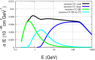
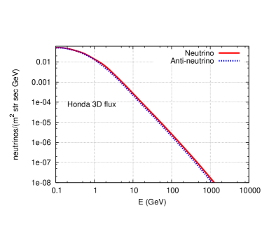
Figure 1: The variation of total CC iron cross section (scaling by a factor of $\frac{1}{56}$) with neutrino energy for both neutrino (left) and anti-neutrino (right) and the variation of atmospheric flux (Honda 3D) with energy (lower) for a fixed zenith angle and azimuthal angle.

In fig. 1, we show the variation of total Charged Current (CC) cross section with neutrino energy for both neutrino and anti-neutrino. In the third plot of this figure, we also show how rapidly the neutrino flux changes with energy.

IV Neutrino oscillation through the Earth matter

The effective Hamiltonian which describes the time evolution of neutrinos in matter can be expressed in flavor basis as

$$H=\frac{1}{2E}\left\{U\left(\begin{array}[]{c c c}0&&\\ &\Delta m_{21}^{2}&\\ &&\Delta m_{31}^{2}\end{array}\right)U^{+}+\left(\begin{array}[]{c c c}A&&\\ &0&\\ &&0\end{array}\right)\right\}$$ (13)

where, $A=G\sqrt{2}N_{e}2E$ is the effective potential of $\nu_{e}$ with electrons, $U$ is the flavor mixing matrix in vacuum (eq. 5), $G$ is the Fermi constant, $N_{e}$ is the electron density of the medium, and $E$ is the neutrino energy.

For a time t, the evolution of neutrino states is given by $\nu(t)=S(t)\nu(0)$ with $S(t)=e^{-iHt}$ for constant matter density. The corresponding effective Hamiltonian for anti-neutrinos is obtained by $U\rightarrow U^{*}$ and $A\rightarrow-A$. To understand the analytical solution one may adopt the so called “one mass scale dominance” (OMSD) frame work: $|\Delta m_{21}^{2}|<<|m_{3}^{2}-m_{1,2}^{2}|$ Peres:2003wd ; Akhmedov:2004ny .

With this OMSD approximation, the survival probability of $\nu_{\mu}$ can expressed as

$$P^{m}_{\mu\mu} = {1-\cos^{2}\theta^{m}_{13}\;{\sin^{2}2\theta_{23}}}$$ (14)

$$\times\sin^{2}\left[1.27\;\left(\frac{{(\Delta m_{31}^{2})}+A+{(\Delta m_{31}^{2})^{m}}}{2}\right)\;\frac{L}{E}\right]$$

$$~{}-~{}\sin^{2}\theta^{m}_{13}\;\sin^{2}2\theta_{23}$$

$$\times\sin^{2}\left[1.27\;\left(\frac{{(\Delta m_{31}^{2})}+A-{(\Delta m_{31}^{2})^{m}}}{2}\right)\;\frac{L}{E}\right]$$

$$~{}-~{}{{\sin^{4}\theta_{23}}}\;{{\sin^{2}2\theta^{m}_{13}\;\sin^{2}\left[1.27\;{(\Delta m_{31}^{2})^{m}}\;\frac{L}{E}\right]}}$$

The mass squared difference ${{{(\Delta m_{31}^{2})^{m}}}}$ and mixing angle ${{\sin^{2}2\theta_{13}^{m}}}$ in matter are related to their vacuum values by

$${(\Delta m_{31}^{2})^{m}}=\sqrt{({(\Delta m_{31}^{2})}\cos 2\theta_{13}-A)^{2}+({(\Delta m_{31}^{2})}\sin 2\theta_{13})^{2}}$$

$$sin2\theta^{m}_{13}=\frac{{{(\Delta m_{31}^{2})}\sin 2\theta_{13}}}{\sqrt{({(\Delta m_{31}^{2})}\cos 2\theta_{13}-A)^{2}+({(\Delta m_{31}^{2})}\sin 2\theta_{13})^{2}.}}$$ (15)

From eq. 14 and 15 it is seen that a resonance in ${{P^{m}_{\mu\mu}}}$ will occur for neutrinos (anti-neutrinos) with NH (IH) when

$$\sin^{2}2\theta_{13}^{m}\rightarrow 1~{}~{}~{}~{}{\rm or,}~{}~{}A=\Delta m^{2}_{31}\cos 2\theta_{13}.$$ (16)

Then resonance energy can be expressed as

$$E=\left[\frac{1}{2\times 0.76\times 10^{-4}Y_{e}}\right]\left[\frac{|\Delta m_{31}^{2}|}{\rm eV^{2}}\cos 2\theta_{13}\right]\left[\frac{\rm gm/cc}{\rho}\right]$$ (17)

Fig. 2 shows how the resonance energy and the average density of the Earth changes with zenith angle.

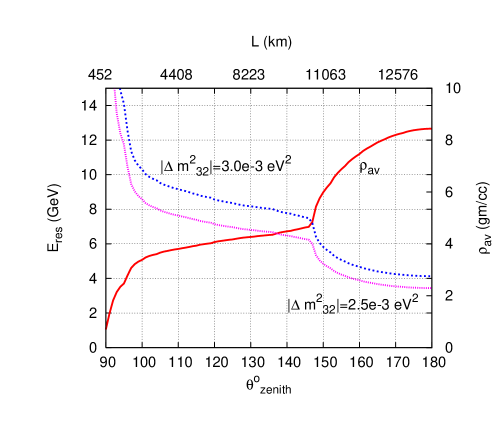
Figure 2: The variation of average density (y2-axis) and the corresponding resonance energy (y1-axis) with zenith angle (x1-axis) and baseline (x2-axis) at $13$ resonance assuming one mass scale dominance approximation. We set $\theta_{13}=10^{\circ}$.

V Role of hierarchy in oscillation probability at different $E_{\nu}$ and $\cos\theta^{\rm zenith}_{\nu}$

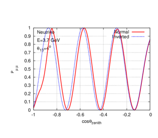
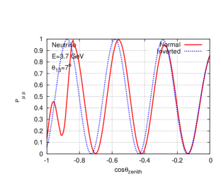
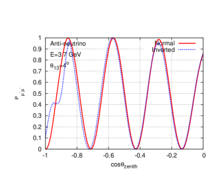
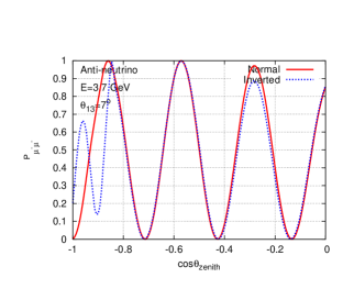
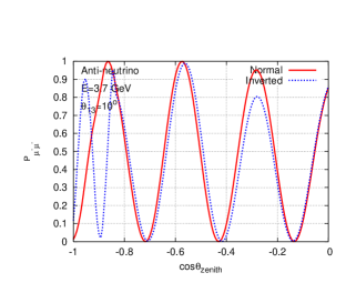
Figure 3: The variation of the $\nu_{\mu}$ (first row) and $\bar{\nu}_{\mu}$ (second row) survival probability with $\cos\theta_{\rm zenith}$ with a fixed energy $E_{\nu}$ = 3.7 GeV for $\theta_{13}=4^{\circ}$ (first column), $7^{\circ}$ (second column), and $10^{\circ}$ (third column). The other oscillation parameters are set at their best-fit values.

The significant difference in survival probabilities between NH and IH arises due to matter resonance. For a neutrino energy $(E_{\nu})$, the corresponding baseline $(L_{\nu})$ or zenith angle ($\theta^{\rm zenith})$ where the resonance occurs, can be understood from fig. 2 for both cases of $\nu_{\mu}$ and $\bar{\nu}_{\mu}$. There are two zones of energy:

1. low energy zone ($E\approx 4$ GeV) for the events through the core of the Earth, and

2. high energy zone ($E\approx 6-8$ GeV) for the events through the mantle of the Earth.

Here we have studied in detail the difference in survival probabilities at different $E_{\nu}$ and $\cos\theta^{\rm zenith}_{\nu}$ using full three flavor oscillation formula with the Earth density profile of PREM modelDziewonski:1981xy . The dependence on the values of the oscillation parameters are also studied in detail. The observations are the following.

The survival probabilities for both NH and IH without matter effect produce a sinusoidal behavior in $L$ for a fixed $E$. In case of non-zero $\theta_{13}$ with NH, it is seen that when $\nu_{\mu}$ with energy $\approx 2-6$ GeV passes through the core of the Earth (density $\approx 12$gm/cc), a large depletion in survival probability $P(\nu_{\mu}\leftrightarrow\nu_{\mu})$ with respect to IH arises due to the increase of $P(\nu_{\mu}\leftrightarrow\nu_{e})$ (see first row of fig. 3). In case of $\bar{\nu}_{\mu}$, it happens for IH (see second row of fig. 3). The important point is that the atmospheric neutrino flux is sufficiently high at this energy range.

Again, there is also a large depletion in survival probability of neutrino (anti-neutrino) for NH (IH) with respect to IH (NH) at the high energy ($\approx 5-10$ GeV) for $-0.75\mathrel{\hbox to0.0pt{\raise 2.15277pt\hbox{$>$}\hss}{\lower 2.15277pt\hbox{$\sim$}}}\cos\theta^{\rm zenith}_{\nu}\mathrel{\hbox to0.0pt{\raise 2.15277pt\hbox{$>$}\hss}{\lower 2.15277pt\hbox{$\sim$}}}-0.40$ as seen in fig. 4, and 5.

This pattern remains almost same over the present allowed range of oscillation parameters.

Though all the above effects diminish rapidly as $\theta_{13}$ goes to zero, there remains a finite difference in the survival probabilities for NH and IH at $\theta_{13}=0$ due to nonzero value of $\Delta m_{21}^{2}$.

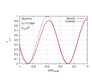
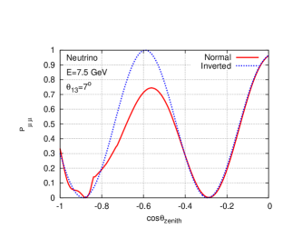
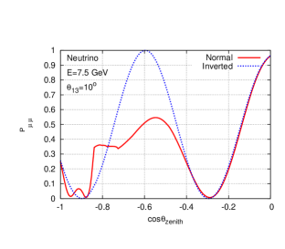
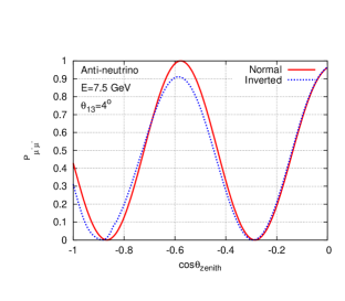
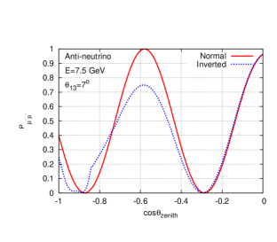
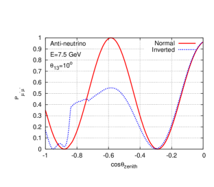
Figure 4: The same plots of fig. 3, but with $E_{\nu}=7.5$ GeV.

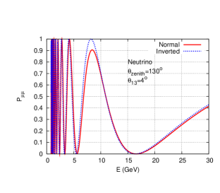
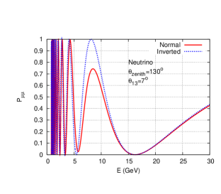
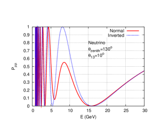
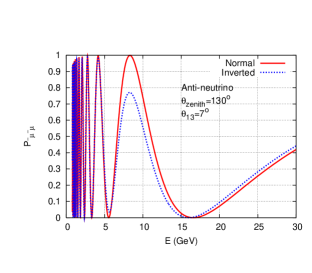
Figure 5: The variation of the $\nu_{\mu}$ (first row) and $\bar{\nu}_{\mu}$ (second row) survival probability with energy for $\theta_{13}=4^{\circ}$ (first column), $7^{\circ}$ (second column), and $10^{\circ}$ (third column) with a typical zenith angle $\theta_{\rm zenith}=130^{\circ}$.

VI Possible systematic uncertainties

The systematic uncertainties may enter into the analysis of data in three steps: i) flux estimation, ii) neutrino interaction, and iii) event reconstruction.

We can divide each of them into two categories: I) overall uncertainties (which are flat with respect to energy and zenith angle), and II) tilt uncertainties (which are function of energy and/or zenith angle).

The uncertainty in flux of category II may arise due to the tilt in its shape with energy and zenith angle. This can be expressed in the following fashion for the case of energy:

$$\Phi_{\delta_{E}}(E)=\Phi_{0}(E)\left(\frac{E}{E_{0}}\right)^{\delta_{E}}\approx\Phi_{0}(E)\left[1+\delta_{E}\log_{10}\frac{E}{E_{0}}\right]$$ (18)

This arises due to the uncertainty in spectral indices. The uncertainty ${\delta_{E}}=$5% and $E_{0}=2$ GeV is considered in analogy with  Kameda ; skthesis2 .

Similarly the flux uncertainty as a function of zenith angle can be expressed as

$$\Phi_{\delta_{z}}(\cos\theta_{z})\approx\Phi_{0}(\cos\theta_{z})\left[1+\delta_{z}\cos\theta_{z}\right]$$ (19)

However, this uncertainty is less $(\approx 2\%)$ Kameda ; skthesis2 than the energy dependent uncertainty.

The experimental systematic uncertainties may come through reconstruction of events. Till now it is not estimated by the simulation of ICAL at INO. However the fact from simulation is that the wrong charge identification possibility is almost zero for the considered energy and zenith angle ranges. Since the detector is symmetric to up and down going events, it is expected that the up/down ratio cancels most of the experimental uncertainties. The quantitative details of the uncertainties of category I (except those arising from the event reconstruction) can be found in Ashie:2005ik .

VII Migration from neutrino to muon energy and zenith angle

In the CC processes, a lepton of same leptonic family of neutrino is produced with addition of some hadrons. Among the leptons, only muon produces a very clean track in ICAL detector and the hadrons produce a few hits around the vertex of the interaction. Our analysis considers only muons, and no hadrons for simplicity.

For a given neutrino energy, the scattering angle and the energy of the muon are related to each other. Again, the neutrino direction is specified by two angles: the polar angle and the azimuthal angle. Therefore, the actual resolution function should be a function of energy and these two angles.

We are only interested in zenith angle which is a complicated function of above two angles. We reduce the above complexity of two angles by constructing a two dimensional resolution function $R(x_{\rm E},x_{\rm zenith})$ for a given neutrino energy with

$$x_{\rm E}=\frac{(E_{\nu}-E_{\mu})}{E_{\nu}},~{}~{}~{}~{}x_{\rm zenith}=(\theta_{\nu}^{\rm zenith}-\theta_{\mu}^{\rm zenith}).$$ (20)

To find the resolution function $R(x_{E},x_{\rm zenith})$, we generate one thousand years un-oscillated atmospheric neutrino data for ICAL. Here, the two angles automatically come in proper way in zenith angle resolution and it should work well in analysis of the atmospheric data. We divide the whole data set into 17 neutrino energy bins (for $E=$0.8-18 GeV) in logarithmic scale. It is also notable that the zenith angle resolution slightly depends on the value of neutrino zenith angle due to the spherical shape of the Earth. To account for this dependence, we divide the whole zenith angle range ($\cos\theta_{z}=-1~{}{\rm to}~{}+1$) into 10 bins for every energy bin. In fig. 6 we show typical resolution functions at low ($\approx 1$ GeV) and high ($\approx 15$ GeV) energy for both neutrinos and anti-neutrinos. Here, we see, the zenith angle resolution improves and energy resolution worsens with increase of energy. The zenith angle resolution is significantly better for $\bar{\nu}_{\mu}$s than $\nu_{\mu}$s.

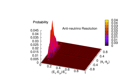
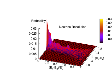
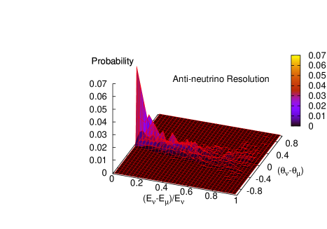
Figure 6: The distribution of probability of the resolution function for neutrino (left) and anti-neutrino (right) at low energy ($\approx 1$ GeV) (top) and at high energy ($\approx 15$ GeV) (bottom).

From the distribution of resolution function (fig. 6), it is clear that the probability is high near zero of $x_{\rm zenith}$ and it rapidly falls as we go far from it. Therefore we use a varying bin size in our analysis for both variables, small near zero and gradually bigger at far values.

How we obtained the number of events in muon energy and zenith angle bins from atmospheric neutrino flux using the above resolution function is described in the following steps.

1. For a given neutrino energy and zenith angle bin, we obtain a distribution of events in a plane with axes $x_{E}=(E_{\nu}-E_{\mu})/E_{\nu}$ and $x_{\rm zenith}=(\theta_{\nu}^{\rm zenith}-\theta_{\mu}^{\rm zenith})$ from a large number of events generated by Nuance as shown in fig. 6. From this distribution we find the probability of getting a muon at a given energy and zenith angle bin dividing the number of events of this bin by the total number of events generated for the particular neutrino energy and zenith angle.

2. The number of events for a given neutrino energy and zenith angle bin is calculated by multiplying the exposed flux with the cross section of this energy. (The cross section is obtained from Nuance as shown in Fig. 1.)

3. To obtain how many events at a particular muon energy and zenith angle bin may come from the number of events of a given neutrino energy and zenith angle bin, we multiply this previously calculated number of events for the given neutrino energy with the probability at this muon energy and angle bin obtained in step 1.

4. The total contribution at a particular muon energy and zenith angle bin is obtained by adding the contribution from all neutrino energy and zenith angle bins. Finally we obtained the total muon events at different energy and zenith angle bins in the considered ranges.

VIII Choices of observables and its variables

The effect of matter on the oscillation probability is a complicated function of $E$, $L$ and the density of medium ($\rho$). From the study of survival probability $P(\nu_{\mu}\leftrightarrow\nu_{\mu})$ and $P(\bar{\nu}_{\mu}\leftrightarrow\bar{\nu}_{\mu})$ in section V, it is clear that the difference between NH and IH is more significant for particular ranges of $E$ and $L$ rather than the range of the combination $L/E$. In case of the combination $L/E$, there remains some $L(E)$ values for some values of $E(L)$ where the difference between NH and IH is insignificant. For these values of $L$ and $E$, it increases the magnitude of statistical errors and eventually kills the significance which comes from the interesting regions of $L$ and $E$. For this reason, we need to consider only important ranges of the baseline $L_{i}$ for each range of energy $E_{i}$.

We may consider the following observables to determine the hierarchy: $u_{i},~{}d_{i},~{}\bar{u}_{i},~{}\bar{d}_{i}$,  ${u_{i}}/{d_{i}}$,  ${\bar{u}_{i}}/{\bar{d}_{i}}$, or any combinations of them, where, $u_{i},~{}d_{i}~{}(\bar{u}_{i},~{}\bar{d}_{i})$ are the up going and down going neutrino (anti-neutrino) events in the interesting $L_{i}-E_{i}$ regions. For down going events we consider the ‘mirror’ $L$ which is exactly equal to that value when the neutrino comes from the opposite direction.

In case of observables with the combination of neutrinos and anti-neutrinos, we will encounter the uncertainty of the ratio ${\nu_{\mu}}/{\bar{\nu}_{\mu}}$ which is $\simeq 1$ at low energy and it increases with energy Honda:2004yz ; Battistoni:2003ju ; Barr:2004br . Since the matter effect and the cross sections for neutrinos and anti-neutrinos are dependent on $E$, the uncertainty in the ${\nu_{\mu}}/{\bar{\nu}_{\mu}}$ ratio may affect significantly in determination of hierarchy for the combined observables.

Firstly, we choose the observables as a ratio of $u$ and $d$ to cancel all the overall uncertainties (discussed in section VI). Secondly, since the magnetized ICAL detector has the capability to distinguish $\mu^{-}$ and $\mu^{+}$, we consider the ratios separately for $\nu_{\mu}$s and $\bar{\nu}_{\mu}$s:

$$A={u}/{d},~{}~{}~{}{\rm and}~{}~{}~{}\bar{A}={\bar{u}}/{\bar{d}}.$$ (21)

In fig. 2, it clearly shows that there is a sudden fall in resonance energy due to a sudden rise in average density of the Earth. We choose two ranges of energy: one for core (vertical events) and another for mantle (slant events). The difference in survival probability between NH and IH can also be seen in figs. 3, and 4 at these two ranges of zenith angle for two typical resonance energy of 3.7 GeV and 7.5 GeV, respectively. The resonance range of energy for a typical value of the zenith angle is also shown in fig. 5.

From the discussion of section III, V and VII, we observed the following :

1. The zenith angle resolution width is large with a peak around zero (fig. 6).

2. From the distribution of the energy resolution, it is clear that a muon of energy $E_{\mu}$ can come from any neutrino having energy $E_{\nu}\mathrel{\hbox to0.0pt{\raise 2.15277pt\hbox{$>$}\hss}{\lower 2.15277pt\hbox{$\sim$}}}E_{\mu}$ with almost equal probability for $E_{\nu}\mathrel{\hbox to0.0pt{\raise 2.15277pt\hbox{$>$}\hss}{\lower 2.15277pt\hbox{$\sim$}}}$ 3 GeV where the deep inelastic events dominate. Again, as the flux falls very rapidly with energy (see fig. 1) and $E_{\nu}\mathrel{\hbox to0.0pt{\raise 2.15277pt\hbox{$>$}\hss}{\lower 2.15277pt\hbox{$\sim$}}}E_{\mu}$ (this is obvious for $E_{\nu}>1$ GeV for targets at rest), the lower value of the energy range will play a crucial role in the results.

The bonus point of these two ranges of zenith angle (vertical and slant) is that the vertical/horizontal uncertainty in flux is minimized and becomes negligible. Among the systematic uncertainties discussed in section VI, we remain with the energy dependent flux uncertainty. Here we will not consider any uncertainty coming from reconstruction of the events. This will be taken care of in near future in GEANT-based studies.

IX $\chi^{2}$ analysis

Here we are interested to find the hierarchy discrimination ability of ICAL@INO at low $\theta_{13}$ using the resonance ranges. It should be noted here that the resonance width falls very rapidly with $\theta_{13}$.

From the earlier works Petcov:2005rv ; Gandhi:2007td ; Indumathi:2004kd it is found that as the energy and the angular resolution width increase the discrimination ability of hierarchy becomes worsened (see fig. 10 of Gandhi:2007td ). In our actual simulation it is found that the width of these resolutions are large (see fig. 6).

We have tried to tackle the problem in the following way. We do not divide the selected ranges. We calculate the total up-going ($u_{i}$) and the total down-going ($d_{i}$) events and then their ratio ($u_{i}/d_{i}$) for each selected range. Finally we perform the chi-square study with these $u_{i}/d_{i}$ ratios of all ranges (see table 1).

For a set of input values of the oscillation parameters, we generate the neutrino events for 1 MTon.year exposure of ICAL detector using the Nuance (see fig. 7). Next we calculate the total $u_{i}$ and the total $d_{i}$ for each considered range of $E_{\mu_{i}}-\cos\theta^{\rm zenith}_{\mu_{i}}$ (see table 1) and then their ratio $u_{i}/d_{i}$. We call it the “experimental data”. The statistical error is estimated by the following formula

$$\sigma_{u_{i}/d_{i}}=\sqrt{\frac{1}{u_{i}}+\frac{1}{d_{i}}}\left(\frac{u_{i}}{d_{i}}\right).$$ (22)

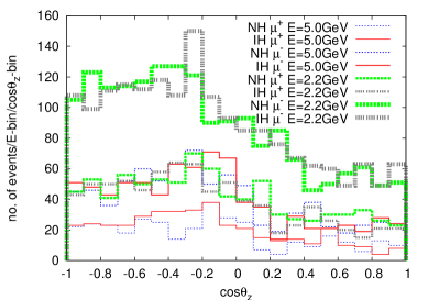
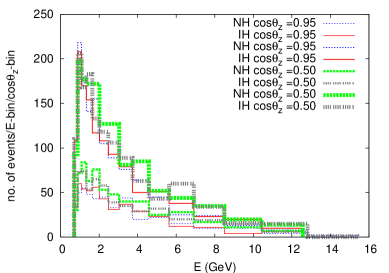
Figure 7: The typical distribution of the number of events with $\cos\theta_{zenith}^{\mu}$ for fixed $E_{\mu}$ (left) and with $E_{\mu}$ for fixed $\cos\theta_{zenith}^{\mu}$ (right). We set $\Delta m_{32}^{2}=-2.5\times 10^{-3}$eV², $\theta_{23}=45^{\circ}$ and $\theta_{13}=7.5^{\circ}$.

We adopt the pull method for chi-square analysis. The theoretical data in chi-square is calculated with the following numerical method.

1. Considering a set of the oscillation parameters and a value of the pull variable for a considered systematic uncertainty (using eq. 18), we obtain the neutrino flux in 200 bins of $E_{\nu}$ and 300 bins of $\cos\theta^{\rm zenith}_{\nu}$. At low energy region the number of oscillation swings with $E$ ($L$) for a fixed $L$ ($E$) are very large (see fig. 3 and 5). Again the difference of the oscillation probabilities between NH and IH changes very rapidly for some ranges of $L$ and $E$. To obtain the accurate oscillation pattern one needs finer binning of $L$ and $E$. We have checked the oscillation plots varying the number of bins for $E_{\nu}$ and $\cos\theta^{\rm zenith}_{\nu}$ and finally fix 200 bins for $E_{\nu}$ and 300 bins for $\cos\theta_{\nu}^{\rm zenith}$. We have used same number of bins to obtain both experimental and theoretical data. The number of events from neutrino to muon energy and zenith angle bins are obtained using the resolution function and the cross section as discussed earlier.

2. Next we calculate the total $u_{i}$ and the total $d_{i}$ separately for each selected range of $E_{\mu_{i}}$-$\cos\theta^{\rm zenith}_{\mu_{i}}$ (see table 1). Then the ratio $u_{i}/d_{i}$ is determined for each range. We call it the “theoretical data”. It should be noted that the number of bins has been changed in chi-square from that of the flux. (The reason is described above.)

3. We calculate the standard chi-square from these “theoretical data”, the above “experimental data” and the “statistical error” (eq. 22) for all ranges. Next the minimization of this chi-sqaure is done with respect to the pull variable to find its best-fit value keeping all other oscillation parameters fixed. Finally the “theoretical data” is again calculated using the best-fit value of the pull variable.

In the last the $\chi^{2}$ is calculated from the final “theoretical data” and the above “experimental data”. The whole process is done to find the $\chi^{2}_{\mu}$ and $\chi^{2}_{\bar{\mu}}$ for $\nu_{\mu}$s and $\bar{\nu}_{\mu}$s, respectively. At the end, we find the total $\chi^{2}=\chi^{2}_{\mu}+\chi^{2}_{\bar{\mu}}$ for the considered set of oscillation parameters.

As discussed in section VI, we consider only neutrino flux uncertainty due to its tilt with energy.

X Resonance ranges in terms of $E_{\mu}$ and $\theta_{\mu}^{\rm zenith}$

The optimization of the ranges by analytical calculation is almost impossible for the complexity in the behavior of survival probability, the smearing of resolution, and the rapid fall of flux with increase of energy.

We calculate the $\chi^{2}$ varying the energy and zenith angle ranges for both NH and IH for a given input of $\theta_{13}$ and type of hierarchy keeping all other oscillation parameters at their best-fit values. Then, we select the ranges where the $\chi^{2}$ difference for NH and IH is the largest. This is done for the input values of $\theta_{13}=4^{\circ},5^{\circ},7^{\circ},10^{\circ}$ and tabulated in table 1. Due to the effect of energy resolution function and the nature of flux, the higher end of the energy range can not be precisely determined. We see, the ranges squeeze rapidly with the decrease of $\theta_{13}$. It should be noted that the ranges determined here has a significant weight of the atmospheric neutrino flux and it is not independent of flux since it is not from the migration of neutrinos to muons only. However, there is no significant change in chi-square if the ranges are changed within few percent of their boundary values.

Resonance ranges in terms of muon energy and zenith angle
$\theta_{13}$	Core		Mantle
	$\cos\theta^{\rm zenith}_{\mu}$	$E_{\mu}$ (GeV)	$\cos\theta^{\rm zenith}_{\mu}$	$E_{\mu}$ (GeV)
	$\mu^{-}$         $\mu^{+}$	$\mu^{-}$         $\mu^{+}$	$\mu^{-}$         $\mu^{+}$	$\mu^{-}$        $\mu^{+}$
$10^{\circ}$	-1.0 to -0.57    -1.0 to -0.72	0.79 to 9.40    0.93 to 7.40	-0.57 to -0.41    -0.68 to -0.46	3.33 to 8.01    5.38 to 8.68
$7^{\circ}$	-1.0 to -0.63    -1.0 to -0.79	1.39 to 10.18    2.07 to 4.59	-0.61 to -0.43    -0.70 to -0.46	4.24 to 6.83    5.38 to 11.94
$4^{\circ}$	-1.0 to -0.50    -1.0 to -0.83	1.63 to 8.68    2.07 to 6.83	-0.48 to -0.30    -0.72 to -0.46	4.59 to 6.31    7.40 to 10.18

Table 1: The resonance ranges of $\cos\theta^{\rm zenith}_{\mu}-E_{\mu}$ for different input values of $\theta_{13}$. The type of input hierarchy is inverted.

XI Marginalization and Results

The neutrino oscillation parameters can not be measured at infinite accuracies. To find at what statistical significance the wrong hierarchy can be disfavored, we calculate the $\chi^{2}$ for both true and false hierarchy varying the oscillation parameters in the following ranges (unless we specify) :

1. $|\Delta m^{2}_{23}|$ : $2.3\times 10^{-3}-2.8\times 10^{-3}$eV²,

2. $\theta_{23}$ : $39^{\circ}-51^{\circ}$, and

3. $\theta_{13}$ : $0^{\circ}-12^{\circ}$.

We set other oscillation parameters at their best-fit values and choose CP-violating phase $\delta=0$. For the data set of each input values of $\theta_{13}$, we used the corresponding resonance range of $E_{\mu}-\cos\theta^{\rm zenith}_{\mu}$.

The marginalized $\chi^{2}$ for both true and false hierarchy as a function of $\theta_{13}$ is shown in fig. 8 for the input of IH and different values of $\theta_{13}$ ($5^{\circ},7^{\circ}$ and $10^{\circ}$). Here the marginalization is done over other two oscillation parameters $|\Delta m_{32}^{2}|$ and $\theta_{23}$. The similar plot is also shown for the input of NH in fig. 9, but with $E_{\mu}-\cos\theta^{\rm zenith}$ ranges as optimized for IH. Finally we show the discrimination sensitivity $\Delta\chi^{2}=\chi^{2}({\rm false})-\chi^{2}({\rm true})$ marginalized over all three oscillation parameters $|\Delta m_{32}^{2}|$, $\theta_{23}$ and $\theta_{13}$ as function of input values of $\theta_{13}$ in fig. 10.

The changes reflected in $\chi^{2}$ with the input of $\theta_{13}$ and the type of hierarchy can be understood from the following facts:

1. Normally the number of events is larger for $\nu_{\mu}$ than $\bar{\nu}_{\mu}$ due to larger $\nu_{\mu}$ cross section. So the $\nu_{\mu}$ contribution to the difference in chi-square due to hierarchy is larger than $\bar{\nu}_{\mu}$. Since $\nu_{\mu}$s are suppressed in NH, the input with IH (larger statistics) will give a larger difference in chi-square and NH can be more easily disfavored than IH. (See fig. 8 and 9 for the input value of $\theta_{13}=10^{\circ}$.) However, once any one type of the hierarchies is disfavored, there remains the other type only. So it is essential to disfavor any one of them.

2. The resolution is better for anti-neutrinos than neutrinos. Again as $\theta_{13}$ decreases, the resonance ranges squeeze very rapidly. This leads to a competition between resolution and statistics resulting a comparable contribution of $\nu_{\mu}$ and $\bar{\nu}_{\mu}$ to chi-square difference for $\theta_{13}\mathrel{\hbox to0.0pt{\raise 2.15277pt\hbox{$<$}\hss}{\lower 2.15277pt\hbox{$\sim$}}}7^{\circ}$ (compare fig. 8 and 9 for the input value of $\theta_{13}=7^{\circ}$).

3. Though there is an appreciable difference in survival probabilities between NH and IH below $\theta_{13}$ value of $5^{\circ}$, the tilt uncertainty with energy kills the difference in chi-squares.

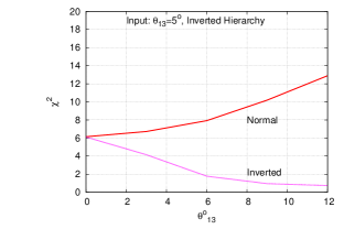
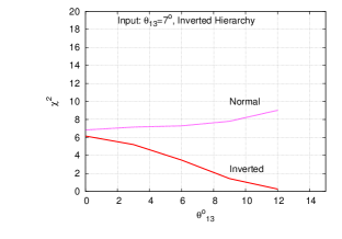
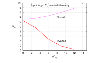
Figure 8: The variation of marginalized $\chi^{2}$ with $\theta_{13}$ for NH and IH for the input of IH and the values of $\theta_{13}$=$5^{\circ}$ (left), $7^{\circ}$ (middle) $10^{\circ}$ (right). The marginalization is done over $|\Delta m_{32}^{2}|=(2.3-2.7)\times 10^{-3}$eV² and $\theta_{23}=39^{\circ}-51^{\circ}$. We consider a uncertainty in tilt factor $\delta_{E}=5\%$ at $E_{\nu}$=2 GeV. The other oscillation parameters are set at their best-fit values (discussed in the text).

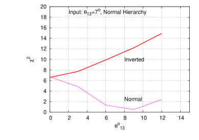
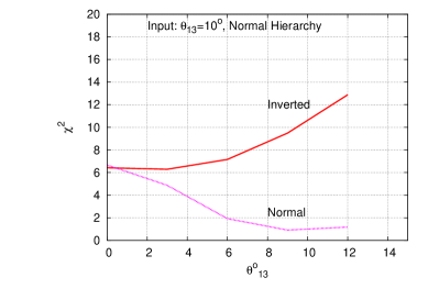
Figure 9: The same plots of fig. 8, but with input of NH and $\theta_{13}$=$7^{\circ}$ (left) and $10^{\circ}$ (right).

Figure 10: The variation of the discrimination sensitivity $\Delta\chi^{2}$ with the input value of $\theta_{13}$ for two marginalization ranges of $|\Delta m_{32}^{2}|$. The range of $\theta_{23}$ is $39^{\circ}$ - $51^{\circ}$. The type of input hierarchy is inverted.

XII Discussion

Here we will discuss some points for the estimation of detector efficiency and the errors that may occur in event reconstruction of the experimental data.

1. One can estimate the efficiency of the ICAL detector in the following procedure. The fiducial volume of the detector can be estimated so that an event with vertex inside this volume can be reconstructed. To reconstruct an event one may need the minimum number of hits $\mathrel{\hbox to0.0pt{\raise 2.15277pt\hbox{$>$}\hss}{\lower 2.15277pt\hbox{$\sim$}}}9$. Therefore, one can estimate the efficiency just neglecting 10 layers from top and bottom and 50 cms from lateral sides. For this into consideration, the efficiency may be roughly

   $$\approx\frac{120~{}{\rm(layers)}\times 4700~{}{\rm cm}\times 1500~{}{\rm cm}}{140~{}{\rm(layers)}\times 4800~{}{\rm cm}\times 1600~{}{\rm cm}}\simeq 79\%.$$

2. For the maximum difference between NH and IH, we find the lowest value of $E_{\mu}\approx 1$ GeV at $\cos\theta^{\rm zenith}_{\mu}=-1$ and the highest value of $E_{\mu}\approx 15$ GeV at $\cos\theta^{\rm zenith}_{\mu}\approx-0.3$. For these cases, we will get number of hits $\mathrel{\hbox to0.0pt{\raise 2.15277pt\hbox{$>$}\hss}{\lower 2.15277pt\hbox{$\sim$}}}12$, and there will be a very high efficiency of filtration and reconstruction of these events in actual experiment.

3. For the muons below the energy of 15 GeV, the charge identification capability of ICAL@INO is $\mathrel{\hbox to0.0pt{\raise 2.15277pt\hbox{$>$}\hss}{\lower 2.15277pt\hbox{$\sim$}}}95\%$ with a magnetic field of 1 Teslaino . Here, we consider only the muons whose reconstruction efficiency is very high and the energy and angle resolutions are within 3-6% for the considered ranges. Moreover, the wrong charge identification possibility is very negligible ino . So one may easily expect that the result estimated in this paper will not change appreciably after GEANTgeant simulation.

XIII Conclusion

We have studied the neutrino mass hierarchy at the magnetized ICAL detector at INO with atmospheric neutrino events generated by the Monte Carlo event generator Nuance(version-3). We have done the analysis in muon energy and zenith angle bins. We have adopted a numerical technique for the migration of number of neutrino events from neutrino energy and zenith angle bins to muon energy and zenith angle bins to find the “theoretical data” in chi-square analysis. The so called “experimental data” are obtained in muon energy and zenith angle bins from the Nuance simulation. The resonance ranges in terms of muon energy and zenith angle are found for different values of $\theta_{13}$. Then we find suitable variables and make a marginalized chi-square analysis using the pull method for both true and false hierarchy. The choice of variables and the pull method minimize the possible systematic uncertainties in the analysis. Finally we find the sensitivity as the difference $\Delta\chi^{2}=\chi^{2}{(\rm false)}-\chi^{2}{(\rm true)}$ as a function of $\theta_{13}$ as shown in fig. 10. It is found that the neutrino mass hierarchy with atmospheric neutrinos can be probed up to a low value of $\theta_{13}\approx 5^{\circ}$ at ICAL@INO by judicious selection of events and observables. Here we have also shown that $>$ 95% CL can be achieved for discrimination of hierarchy at $\theta_{13}\mathrel{\hbox to0.0pt{\raise 2.15277pt\hbox{$>$}\hss}{\lower 2.15277pt\hbox{$\sim$}}}5^{\circ}$ in a 1 Mton-year exposure of ICAL detector.

References

- (1) Review of Particle Physics, S. Eidelman et al., Phys. Lett. B 592 (2004) 1.
- (2) B. Pontecorvo, JETP 6 (1958) 429; 7 (1958) 172; Z. Maki, M. Nakagawa and S. Sakata, Prog. Theor. Phys. 28, 870 (1962).
- (3) T. Schwetz, Phys. Scripta T127 (2006) 1 [arXiv:hep-ph/0606060].
- (4) For reviews see, for example, R. N. Mohapatra et al., arXiv:hep-ph/0412099; A. De Gouvea, Mod. Phys. Lett. A 19, 2799 (2004) [arXiv:hep-ph/0503086].
- (5) A. de Gouvea, J. Jenkins and B. Kayser, Phys. Rev. D 71, 113009 (2005) [arXiv:hep-ph/0503079].
- (6) M. G. Zois, FERMILAB-MASTERS-2004-06
- (7) Y. Yamada [T2K Collaboration], Nucl. Phys. Proc. Suppl. 155, 207 (2006).
- (8) J. Kisiel [ICARUS Collaboration], Acta Phys. Polon. B 36, 3227 (2005).
- (9) R. Ray, Nucl. Phys. Proc. Suppl. 154, 179 (2006).
- (10) G. Horton-Smith [Double Chooz Collaboration], AIP Conf. Proc. 805, 142 (2006).
- (11) C. K. Jung, arXiv:hep-ex/0005046.
- (12) H. Back et al., arXiv:hep-ex/0412016.
- (13) K. Nakamura, Int. J. Mod. Phys. A 18, 4053 (2003).
- (14) F. Di Capua [OPERA Collaboration], PoS HEP2005, 177 (2006).
- (15) See http://www.imsc.res.in/ino.
- (16) V. Arumugam et al. [INO Collaboration], INO-2005-01
- (17) V. Barger, D. Marfatia, K. Whisnant, Phys. Rev. D 65 (2002) 073023; P. Lipari, Phys. Rev. D 61 (2000) 113004; P. Huber, W. Winter, Phys. Rev. D 68 (2003) 037301.
- (18) S. K. Agarwalla, A. Raychaudhuri and A. Samanta, Phys. Lett. B 629, 33 (2005) [arXiv:hep-ph/0505015].
- (19) J. Burguet-Castell, et al., Nucl. Phys. B 608 (2001) 301; P. Huber, M. Lindner, W. Winter, Nucl. Phys. B 645 (2002) 3; V. Barger, D. Marfatia, K. Whisnant, Phys. Rev. D 65 (2002) 073023.
- (20) S. T. Petcov and T. Schwetz, Nucl. Phys. B 740, 1 (2006) [arXiv:hep-ph/0511277].
- (21) R. Gandhi, P. Ghoshal, S. Goswami, P. Mehta, S. U. Sankar and S. Shalgar, Phys. Rev. D 76 (2007) 073012 [arXiv:0707.1723 [hep-ph]].
- (22) D. Indumathi and M. V. N. Murthy, Phys. Rev. D 71, 013001 (2005) [arXiv:hep-ph/0407336].
- (23) R. Gandhi, P. Ghoshal, S. Goswami, P. Mehta and S. Uma Sankar, Phys. Rev. D 73, 053001 (2006) [arXiv:hep-ph/0411252].
- (24) T. Maeno et al. [BESS Collaboration], Astropart. Phys. 16, 121 (2001) [arXiv:astro-ph/0010381].
- (25) J. Alcaraz et al. [AMS Collaboration], Phys. Lett. B 461, 387 (1999) [arXiv:hep-ex/0002048].
- (26) M. Honda, T. Kajita, K. Kasahara and S. Midorikawa, Phys. Rev. D 70, 043008 (2004) [arXiv:astro-ph/0404457].
- (27) D. Casper, Nucl. Phys. Proc. Suppl. 112, 161 (2002) [arXiv:hep-ph/0208030].
- (28) O. L. G. Peres and A. Y. Smirnov, Nucl. Phys. B 680 (2004) 479 [arXiv:hep-ph/0309312].
- (29) E. K. Akhmedov, R. Johansson, M. Lindner, T. Ohlsson and T. Schwetz, JHEP 0404 (2004) 078 [arXiv:hep-ph/0402175].
- (30) A. M. Dziewonski and D. L. Anderson, Phys. Earth Planet. Interiors 25, 297 (1981).
- (31) G. Battistoni, A. Ferrari, T. Montaruli and P. R. Sala, arXiv:hep-ph/0305208.
- (32) G. D. Barr, T. K. Gaisser, P. Lipari, S. Robbins and T. Stanev, Phys. Rev. D 70, 023006 (2004) [arXiv:astro-ph/0403630].
- (33) J. Kameda, Ph.D. thesis, ”http://www-sk.icrr.u-tokyo.ac.jp/doc/sk/pub/”.
- (34) M. Ishitsuka, Ph.D. thesis, ”http://www-sk.icrr.u-tokyo.ac.jp/doc/sk/pub/”.
- (35) Y. Ashie et al. [Super-Kamiokande Collaboration], Phys. Rev. D 71 (2005) 112005 [arXiv:hep-ex/0501064].
- (36) GEANT – Detector Simulation and Simulation Tool, CERN Program Library Long Wri-up W5013, March 1994, http://wwwasd.web.cern.ch/wwwasd/cernlib/version.html