New approach in the extracting of parton densities, based on the parameterized solution of inverse Mellin technique

Abstract

We analysis the sea quark densities, based on the constituent quark model. To perform a direct fit with available experimental data, the parameterized Inverse Mellin technique is used. The calculation is extended to the NLO approximation for the singlet and non-singlet cases in DIS phenomena. We employ the approach of complete RG improvement(CORGI) where one is forced to identify and resum to all-orders RG-predictable ultraviolet logarithm terms which truly build the Q-dependence of QCD observable. The results are compared with the standard approach of perturbative QCD in the ${\overline{MS}}$ scheme with a physical choice of scale. The results in the CORGI approach indicate a better agreement to the data.

I Introduction

One of the feature of strong interaction field which is investigated by many phenomenological model is the Quark parton model. To construct the hadron structure from the parton densities, we use from the constituent quark model Hwa-81 (1) which seems to give us a better insight. A constituent parton is defined as a cluster of valence quarks accompanied by a cloud of sea quarks and gluons. They have been referred to as valons. It can be considered as a bound state in which, for instance, a proton consists of three valons, two U-valons and one D-valon which, on the one hand, interact with each other in a way that is characterized by the valon wave function and which on the other hand contribute independently in an inclusive hard collision with a $Q^{2}$ dependence that can be calculated in QCD at high $Q^{2}$. These valons thus carry the quantum numbers of the respective valence quarks. Hwa Hwa-80 (2) found evidence for the valons in the deep inelastic neutrino scattering data, suggested their existence and applied it to a variety of phenomena. Hwa Hwa-80-II (3) has also successfully formulated a treatment of the low-$P_{T}$ reactions based on a structural analysis of the valons. Some papers can be found in which the valon model has been used to extract new information for parton distributions and hadron structure functions in unpolarized and polarized casesArash-I (4).

To improve and increase the reliability of the perturbative QCD calculation, we try to use the Complete Renormalization Group Improvement (CORGI) approach which is related to the long standing problem of renormalization ($\mu$)and factorization (M) scale dependence in QCD predictions. Usually in Renormalization Group(RG)-improving perturbation theory, it is assumed that these scales are related to the physical scale Q and ${\mu}$= M=Q is normally chosen. The resulting fixed-order predictions depend on the choice of scales. If instead one insists that these dimentionful scales are independent of Q, one is forced to identify and resum to all-orders RG-predictable ultraviolet logarithms of Q which truly build the Q-dependence. In so doing all dependence on ${\mu}$ and M disappear. This Complete RG Improvement (CORGI) approach has previously been applied to the single scale case where there is only ${\mu}$-dependence Max-98 (5). It is then extended to the more complicated pattern of logarithms involved in the two scales problem of moments of structure functions max-mir-00 (6). In this approach the standard perturbative series of QCD observable is reconstructed in terms of scheme-invariant quantities. So it is expected to get more accurate results compared to those obtained in the standard perturbative QCD approach.

Finally, in order to obtain directly all unknown parameters of the model, just by using the available experimental data, we use from the Inverse Mellin Technique, not in a numerical form but in a parameterized form. Usually one uses numerical computation to extract parton densities from their moments, but we believe that the parameterized Inverse Mellin technique is a mathematically powerful tool which produces more reliable results than those obtained from the customary numerical method. Using the symmetry properties of the inverse Mellin transformation and also a Taylor expansion of the integrand function, we are able to obtain the parameterized solution.

II Phenomenological constituent quark model

The idea of quark cluster is not new. In this model, the hadron is envisaged as a bound state of valence quark clusters. For example the bound state of $\pi^{-}$ consists of a“anti-up” and “down” constituent quarks. In the static problems there is a little difference between the usual constituent quarks and the valons, since the point-like nature of the constituent quarks is not a crucial aspect of the description, and has been assumed mainly for simplicity. But, in the scattering problems it is important to recognize that the valons, being clusters of partons, can not easily undergo scattering as a whole. The fact that the bound-state problem of the nucleon can be well described by three constituent quarks implies that the spatial extensions of the valons do not overlap appreciably. A physical picture of the nucleon in terms of three valons is then quite analogous to the usual picture of the deuteron in terms of two nucleons.

To facilitated the phenomenological analysis the following simple form for the exclusive constituent quark inside the proton is assumed Hwa-81 (1)

$${G_{UUD/p}(y_{1},y_{2},y_{3})=g\,(y_{1}y_{2})^{\alpha}\,y_{3}^{\beta}\,\delta(y_{1}+y_{2}+y_{3}-1),}$$

where $\alpha$ and $\beta$ are two free parameters and $y_{i}$ is the momentum fraction of the i’th constituent quark. The $U$ and $D$ type inclusive constituent quark distributions can be obtained by double integration over the specified variables:

$$G_{U/p}(y) =\int dy_{2}\,\int dy_{3}\,G_{UUD/p}(y,y_{2},y_{3})=$$ (1)

$$gB(\alpha+1,\beta+1)\,y^{\alpha}\,(1-y)^{\alpha+\beta+1},$$

$$G_{D/p}(y) =\int dy_{1}\,\int dy_{2}\,G_{UUD/p}(y_{1},y_{2},y)=$$ (2)

$$gB(\alpha+1,\alpha+\beta+2)\,y^{\beta}\,(1-y)^{2\alpha+1}.$$

The normalization parameter $g$ has been fixed by requiring

$$\int_{0}^{1}G_{U/p}(y)\,dy=\int_{0}^{1}G_{D/p}(y)\,dy=1,$$ (3)

and is equal to $g=[B(\alpha+1,\beta+1)\,B(\alpha+1,\alpha+\beta+2)]^{-1}$, where $B(m,n)$ is the Euler-beta function. Hwa and Yang Hwa-02 (7) have recalculated the unpolarized valon distribution inside the proton with minimization method, using direct fit to CTEQ parton distributions, and have reported a new values of $\alpha$ and $\beta$ which are found to be $\alpha=1.76$ and $\beta=1.05$.

This model suggests that the structure function of a hadron involves a convolution of two distributions. Constituent quark distributions in the proton and structure function for each constituent quark so as

$$F_{2}^{p}(x,Q^{2})=\sum_{v}\int_{x}^{1}dy\,G_{v/p}(y)\,F_{2}^{v}(z={x\over y},Q^{2})\,.$$ (4)

We shall also assume that the three valons carry all the momentum of the proton. This assumption is reasonable provided that the exchange of very soft gluons is responsible for the binding. Eq. (4) involves also the assumption that in the deep inelastic scattering at high $Q^{2}$ the valons are independently probed, since the shortness of interaction time makes it reasonable to ignore the response of the spectator valons. Thus, through Eq. (4) we have broken up the hadron structure problem into two parts. One part represented by $G_{v/p}(y)$, describes the wave functions of the proton in the valon representation. It contains all the hadronic complications due to the confinement. It is independent of $Q^{2}$ or the probe. The other part represented by $F_{2}^{v}(z={x\over y},Q^{2})$, describes the virtual QCD processes of the gluon emissions and quark-pair creation. It refers to an individual valon independent of the other valons in the proton and consequently also independent of the confinement problem. It depends on $Q^{2}$ and the nature of the probe.

Since the calculation in moment n-space is easier than the calculation in x-space, we work with to the moments of the distribution, defining

$$M_{2,3}(n,Q^{2})=\int_{0}^{1}dx\,x^{n-2}\,\left\{\begin{array}[]{c}F_{2}\\ xF_{3}\end{array}\right\}(x,Q^{2}),$$

It then follows from Eq. (4) that

$$M^{N}(n,Q^{2})=\sum_{v}M_{v/N}(n)\,M^{v}(n,Q^{2}).$$ (5)

The distributions we shall calculate (all referring to the proton) are those for sea quarks $xu_{sea}(x)=x\bar{u}(x)=xd_{sea}=x\bar{d}(x)=xs(x)=x\bar{s}(x)=\cdots$, which we shall generally denote by $x\bar{q}(x)$. Its moment is denoted by $M_{sea}(n,Q^{2})$ or equivalently $M_{sea}(n,s)$ where $s$ is evolution parameter which in leading order is defined by

$$s=\log{{\log{Q^{2}/\Lambda_{\overline{MS}}^{2}}}\over{\log{Q_{0}^{2}/\Lambda_{\overline{MS}}^{2}}}}\,,$$ (6)

and generally at any required order is defined by

$$s=\log{{a(Q_{0}^{2})}\over{a(Q^{2})}}\,,$$ (7)

where $a(Q^{2})$ is related to the strong coupling constant by $a(Q^{2})=\alpha_{s}(Q^{2})/4\pi$ . Using Eq. (5), we obtain

$$M_{sea}(n,s) = {1\over 2f}\left[2U(n)+D(n)\right]$$ (8)

$$\times\left[M^{S}(n,s)-M^{NS}(n,s)\right],$$

where $M^{S}$ and $M^{NS}$ are singlet and non-singlet evolution function given in leading order by

$$M^{NS}(n,s)=\exp{(-d_{NS}\,s)},$$

$$M^{S}(n,s)={1\over 2}(1+\rho)\,\exp{(-d_{+}\,s)}+{1\over 2}(1-\rho)\,\exp{(-d_{-}\,s)}.$$

These moments are the leading order solution of the renormalization group equation in QCD. The anomalous dimensions, d and other associated parameters are defined in Hwa-80-II (3).

We shall from now indicate the moment of sea quark densities by $M(n,Q^{2})$. In the NLO approximation, we havemom-NLO (8)

$$\begin{array}[]{rl}M^{NS}(n,Q^{2})=&\left[1+{\alpha_{s}(Q^{2})-\alpha_{s}(Q_{0}^{2})\over 4\pi}\left({\gamma_{1}^{NS}\over 2\beta_{0}}-{\beta_{1}\gamma_{0}^{qq}\over 2\beta_{0}^{2}}\right)\right]\\ \\ &\left({\alpha_{s}(Q^{2})\over\alpha_{s}(Q_{0}^{2})}\right)^{\gamma_{0}^{qq}/2\beta_{0}},\end{array}$$

and

$$\begin{array}[]{rl}\displaystyle\pmatrix{M^{S}(n,Q^{2})\cr M^{g}(n,Q^{2})}&=\displaystyle\left[P_{-}-{1\over 2\beta_{0}}{\alpha_{s}(Q_{0}^{2})-\alpha_{s}(Q^{2})\over 4\pi}P_{-}.\gamma.P_{-}\right.\vspace*{5mm}\\ &\displaystyle-\left({\alpha_{s}(Q_{0}^{2})\over 4\pi}-{\alpha_{s}(Q^{2})\over 4\pi}\left({\alpha_{s}(Q^{2})\over\alpha_{s}(Q_{0}^{2})}\right)^{(\lambda_{+}-\lambda_{-})/2\beta_{0}}\right)\vspace*{5mm}\\ &\displaystyle\left..{P_{-}.\gamma.P_{+}\over 2\beta_{0}+\lambda_{+}-\lambda_{-}}\right]\left({\alpha_{s}(Q^{2})\over\alpha_{s}(Q_{0}^{2})}\right)^{\lambda_{-}/2\beta_{0}}+(+\longleftrightarrow-).\end{array}$$ (9)

The parameters ($\gamma$’s, $\lambda$’s, $\beta$’s and $P$’s) are defined in references mom-NLO (8, 9, 10, 11, 12).

We will discuss how we can extend and improve the precision of the calculation by direct use of available experimental data mishra (13), without referring to the input scales $Q_{0}$ and $\Lambda_{\overline{MS}}$. In this sense, we extract parton densities from the analytical moments of densities. A method devised to deal with this situation is to perform the integration of the inverse Mellin transformation in parameterized form which will be explained in section 4.

III Renormalization and factorization scale dependence

The problem of renormalization scheme dependence in QCD perturbation theory remains on obstacle to making precise tests of the theory. It was pointed out Max-98 (5) that the renormalization scale dependence of dimensionless physical QCD observables, depending on a single energy scale $Q$, can be avoided provided that all ultraviolet logarithms which build the physical energy dependence on $Q$ are resummed. This was termed complete Renormalization Group (RG)-improvement approach. For a single case of a dimensional observable ${{\cal{R}}(Q)}$ with

$${{\cal{R}}(Q)}=a+{r_{1}}{a^{2}}+{r_{2}}{a^{3}}+\ldots+{r_{n}}{a^{n+1}}+\ldots\;.$$ (10)

The RS can be labelled by the non-universal coefficients of the beta-function and $\Lambda_{RS}$ Stevenson (14). Self-consistency of perturbation theory that is the derivative of N-th order approximant ${{\cal{R}}(Q)}$ with respect to the scheme labelled parameters, is of higher order than the approximant itself, will yields partial differential equations for coefficients $r_{2}$, $r_{3}$ and … with respect to non-universal coefficients of $\beta$-function and $r_{1}$ coefficient. On integration of these partial differential equations, one finds max-mir-00 (6)

$${r_{2}}({r_{1}},{c_{2}})={r_{1}}^{2}+c{r_{1}}+{X_{2}}-{c_{2}}$$

$${r_{3}}({r_{1}},{c_{2}},{c_{3}}) = {r_{1}}^{3}+{5\over 2}c{r_{1}}^{2}+(3{X_{2}}-2{c_{2}}){r_{1}}+$$

$${X_{3}}-{1\over 2}{c_{3}}$$

$$\hskip 156.49014pt\vdots\;\;.$$ (11)

General Structure is as follows

$${r_{n}}({r_{1}},{c_{2}},{\ldots},{c_{n}}) = {{\hat{r}}_{n}}({r_{1}},{c_{2}},{\ldots},{c_{n-1}})+{X_{n}}$$

$$-{c_{n}}/(n-1);$$

where $X_{n}$ are Q-independent and RS-invariant and are unknown unless a complete $N^{n}LO$ calculation has been performed. Now we can reformulated $R(Q)$ as it follows

$${\cal{R}}(Q)=a+{r_{1}}{a^{2}}+({r}_{1}^{2}+c{r_{1}}+{X_{2}}-{c_{2}}){a^{3}}+{\ldots}\;.$$ (12)

Given a NLO calculation, ${r_{1}}$ is known but ${X_{2}},{X_{3}},{\ldots}$ are unknown. Thus the complete subset of known terms in Eq. (12) at NLO is

$${a_{0}}{\equiv}a+{r_{1}}{a^{2}}+({r}_{1}^{2}+c{r_{1}}-{c_{2}}){a^{3}}+{\ldots}\;,$$ (13)

and it is RS-invariant. Choose $r_{1}=0,c_{2}=c_{3}==c_{n}=0$ we obtain $a_{0}=a$ max-mir-00 (6). At NNLO calculation $X_{2}$ is unknown. Further infinite subset of terms are known and can be resummed to all orders,

$${X_{2}}{a_{0}}^{3}={X_{2}}{a^{3}}+3{X_{2}}{r_{1}}{a^{4}}+\ldots\;.$$ (14)

Finally we will arrive at

$${\cal{R}}(Q)={a_{0}}+{X_{2}}{a_{0}}^{3}+{X_{3}}{a_{0}}^{4}+{\ldots}+{X_{n}}{a_{0}}^{n+1}+{\ldots}\;,$$ (15)

which in fact is the expansion of QCD observable in Complete RG-Improvement (CORGI) approach. Here $a_{0}=a(0,0,0,)$ is the coupling in this scheme and satisfies

$$\frac{1}{a_{0}}+c{\ln}\left(\frac{c{a_{0}}}{1+c{a_{0}}}\right)=b{\ln}\left(\frac{Q}{{\Lambda}_{\cal{R}}}\right)\;.$$ (16)

In fact the solution of this transcendental equation can be written in closed form in terms of the Lambert $W$-function lam1 (15, 16), defined implicitly by $W(z)\exp(W(z))=z$,

$${a_{0}} = -\frac{1}{c[1+W(z(Q))]}$$

$$z(Q) {\equiv} -\frac{1}{e}{\left(\frac{Q}{{\Lambda}_{\cal{R}}}\right)}^{-b/c}\;.$$ (17)

where $b$ and $c$ are the first two universal terms of QCD $\beta$-function.

Each term in Eq. (15) involves a resummation of infinite terms at specified order. For instance, the first term in this equation, $a_{0}$, is representing a resummation over NLO contributions and the second term, $X_{2}a_{0}^{3}$, a resummation over the NNLO contributions of all terms in Eq.(10). The advantage of CORGI approach is that not only each term in the related perturbative series is scheme independent but also because it involves a resummation of RG-predictable terms, it should yield more accurate approximations than the standard truncation of Eq. (10).

If we intend to employ the CORGI approach to extract sea quark densities in the LO approximation we need just to change the RG-coupling constant $a$ to $a_{0}$ which exists in definition of evolution parameter $s$ that is defined by $s=\log{{a(Q_{0}^{2})}\over{a(Q^{2})}}$. We should note that in the definition of $a_{0}$, the $\Lambda_{\cal R}$ quantity will depend on $r_{1}$ and this coefficient is observable-dependent.

To do the NLO calculation in the standard approach to extract sea quark densities, it is necessary to have anomalous dimensions and Wilson coefficient functions for the singlet and non-singlet sectors involved, for instance, deep inelastic of lepton-nucleon scattering or $e^{+}e^{-}$ annihilation. According to Eqs. (II,9) and following mom-NLO (8, 9, 10, 11), the results for singlet and non-singlet moments can be obtained and the final results for sea quark density will be independent of the chosen observable.

To employ the CORGI approach in higher order, we should use the general form for moments max-mir-02 (17):

$$\begin{array}[]{l}\displaystyle M(n,Q^{2})=\vspace*{3mm}\\ \displaystyle A(n)\left({ca_{0}(n)\over 1+a_{0}(n)}\right)^{d(n)/b}(1+X_{2}(n)a_{0}^{2}(n)\\ \\ +X_{3}(n)a_{0}^{3}(n)+\cdots+X_{k}(n)a_{0}^{k}(n)+\cdots),\end{array}$$

where $a_{0}(n)$ is defined by Eq. (17) and $X_{k}(n)$ are the scheme invariant constants which where introduced before. For the case of dependence on $\mu$ and $M$ scales we havemax-mir-02 (17)

$$\Lambda_{\cal R}=\Lambda_{\overline{MS}}\left({2c\over b}\right)^{-c/b}\exp{\left({d_{1}(n)\over bd(n)}+{r_{1}(n)\over d(n)}\right)},$$ (18)

where $d_{1}(n)$ is the $\overline{MS}$ NLO anomalous dimension coefficient, and $r_{1}(n)$ is computed in the $\overline{MS}$ scheme with $\mu=Q$. The $(2c/b)^{-c/b}$ factor corresponds to the standard convention for defining $\Lambda_{\overline{MS}}$. In the NLO approximation of the CORGI approach , we just need to keep the first two terms in the above series. The $X_{2}(n)$ is defined by max-mir-02 (17)

$$X_{2}(n) = {-1\over 2}-{b\over 2d(n)}r_{1}^{2}(n)-{cd_{1}(n)\over 2b}+{d_{2}(n)\over 2b}+$$ (19)

$${c_{2}d(n)\over 2b}+r_{2}(n).$$

The NLO CORGI invariant $X_{2}(n)$ can be computed from the $\overline{MS}$ results for $r_{1}(n)$, $r_{2}(n)$, $d_{1}(n)$ $\&$ $d_{2}(n)$ ver-01 (10). We should note that in Refs.max-mir-00 (6, 17) the adopted conventions for defining the anomalous dimensions and coefficient functions are different with respect to other references. To obtain $M(n,Q^{2})$ for the singlet case, we need to diagonalize the anomalous dimension matrix. To avoid this we restrict ourselves just to considering the non-singlet case.

IV Fitting methods- Parameterized Solution

In order to check the validity of the valon model and also to increase its ability to get more reliable parton densities (sea quark densities in our case), we make use of a method which we call $\beta$-fitting.

We assume the following phenomenological form for the sea quark densities:

$$x\bar{q}(x,Q^{2})=a\,x^{b}\,(1-x)^{c}\,(1+dx+e\sqrt{x}).$$ (20)

The parameters $a$, $b$, $c$, $d$ and $e$ are generally $Q^{2}$-dependent. The motivation for choosing this functional form is that the term $x^{b}$ controls the low-$x$ behavior of sea densities, and $(1-x)^{c}$ that at large values of $x$. The remaining polynomial factor accounts for the additional medium-$x$ values.

The results of calculation indicates that the chosen functional form will yield a better fitting for the moment of the distribution, than that assumed for the sea quark distribution in RefHwa-80 (2).

Using the Mellin transformation

$$M(n,Q^{2})=\int_{0}^{1}x^{n-2}\,x\bar{q}(x,Q^{2})\,dx,$$ (21)

where $x\bar{q}(x,Q^{2})$ has been defined in Eq. (20), we arrive at

$$M{(n,Q^{2})} = a\,\Gamma(1+c)\,\left({\Gamma(-1+b+n)\over\Gamma(b+c+n)}\right.$$

$$\left.+{e\,\Gamma(-{1\over 2}+b+n)\over\Gamma({1\over 2}+b+c+n)}+{d\,\Gamma(b+n)\over\Gamma(1+b+c+n)}\right).$$

The unknown parameters $a,b,c,d$ and $e$ in Eq. (LABEL:mom-disfun) are obtained from the fitting of analytical results of moments in Eq. (8) over the parameterized form of this equation which is in terms of $\Gamma$ or eventually Euler Beta functions. So we call this method $\beta$-fitting. The quantities $M^{S}$ and $M^{NS}$ in Eq. (8), are known analytically from QCD calculation and moments of valon distributions, $U(n)$ and $D(n)$, are defined in Hwa-81 (1).

Now to report directly all exist parameters, just by using the available experimental data, we can use from the Inverse Mellin Technique, not in a numerical form but in a parameterized form. For this propose, we take the Inverse Mellin of moment of distribution in complex space:

$$F(x,Q^{2})={1\over 2\pi i}\int_{c-i\infty}^{c+i\infty}{dn\over x^{n-1}}\,M(n,Q^{2}).$$ (23)

Since the variable $c$ should be placed on the right hand side of all singularities and considering this point that all singularities of moments will occur for $n$ less than $2$, so we choose $c$ equal to $3$. The integrated interval was first $[3-10i,3+10i]$. If we choose the interval $[3-20i,3+20i]$, there will be a difference only of order about $10^{-5}$ with respect to last interval.

Since the function $M(n,Q^{2})$ is not a simple function, our machine will not be able to compute Eq. (23). We use from this point that this integral with respect to real axis, is symmetric. So first we do integral for interval $[c=c+0i,c+mi]$ where the final result is twice this result.

The technique which we used to integrate the $M(n,Q^{2})$ in (23) is that we first choose a small interval, say $[c+0i,c+2\epsilon i]$. Then we expand $M(n,Q^{2})$ about $c+\epsilon i$. If $\epsilon$ is small enough, we can keep just the first term of this expansion. In next step, we repeat the calculation for interval $[c+2\epsilon i,c+4\epsilon i]$ and expand $M(n,Q^{2})$ about $c+3\epsilon i$. Repeating this procedure and adding all results, we are able to calculate Eq. (23) completely in parameterized form.

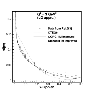
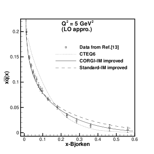
Figure 1: The results of Inverse Mellin (IM) technique for the standard and CORGI approaches in the LO approximation.

Figure 2: The results of Inverse Mellin (IM) technique for NLO approximation in both of Standard and CORGI approach.

Now we are in a position (by direct fitting of $F(x,Q^{2})$ from Eq. (23) over available experimental data mishra (13)) to obtain the unknown parameters of this function which include $\alpha$ and $\beta$ (valon parameters) and $Q_{0}$ and $\Lambda_{\overline{MS}}$. These last two parameters occur in the definition of the evolution parameter, $s$. Unfortunately, from this direct fitting, we were not able to get reliable results for the unknown parameters. To overcome this difficulty, we inserted the values of the valon parameters $\alpha$ and $\beta$, quoted from Hwa-02 (7), in the distribution function, so this function will just depend on the $Q_{0}$ and $\Lambda_{\overline{MS}}$ parameters, $f\equiv{f(x,Q_{0},\Lambda_{\overline{MS}})}$. To get the best fitting $\chi^{2}$ value, we multiplied this function by an auxiliary term, $A\,x^{B}\,(1-x)^{C}$ and fitted to obtain the unknown parameters $Q_{0}$, $\Lambda_{\overline{MS}}$, $A$, $B$ and $C$. We did the fitting for , $Q^{2}=3\ GeV^{2}$ and $Q^{2}=5\ GeV^{2}$ where we assumed a number of active quark flavours $N_{f}=3$ and took an average of the fitted parameters. The difference between the fitted parameters can be reported as an error of the calculations. The results are tabulated in Table I.

One way to check the validity of calculations is to extract the quark densities using the phenomenological form in Eq.(20). For this purpose, we went back to the $\beta$-fitting method and repeated those calculations, but this time with the extracted values of $Q_{0}$ and $\Lambda_{\overline{MS}}$ ($\alpha$ and $\beta$ taken from RefHwa-02 (7). As a consequence, new values for parameters contained in Eq.(20) will be obtained. In order to get the best fit, we again multiply Eq.(20) by the auxiliary term $A\,x^{B}\,(1-x)^{C}$, as we did in the inverse Mellin Technique. We refer to this result as the “improved Inverse Mellin (IM) technique”. These new results in two different standard and CORGI approaches and their comparison with experimental data are plotted in Fig.1 and Fig.2. As can be seen from Fig.2 the result in CORGI approach will show better behavior in small $x$ values.

Table 1: Numerical values of the unknown parameters, resulted from the parameterized solution of the inverse Mellein transform technique in the LO approximation.

Fitting parameters
A	$3.358\pm 0.124$
B	$0.134\pm 0.033$
C	$-3.345\pm 0.264$
$Q_{0}$	$0.422\pm 0.009$(Gev)
$\Lambda_{\over{MS}}$	$0.252\pm 0.004$(Gev)

V Conclusions

Constituent quark model or valon model as a good candidate to describe deep inelastic scattering and to extract sea quark densities inside the nucleon is used. The model bridges the gap between the bound state problem and the scattering problem for hadrons. It is possible to use this model in the LO and NLO approximations, using two different standard and CORGI approaches. The most important motivation for the CORGI approach is that by completely resumming all the UV logarithms, one correctly generates the physical dependence of the moments ${\cal{M}}(n,{Q}^{2})$ on the DIS energy scale $Q$.

In order to get the unknown parameters of the model from the fitting over the available experimental data, parameterized Inverse Mellin technique is used. The compared results will show that the CORGI approach indicates better consistency with available experimental data. An alternative “$\beta$-fitting” method which is based on using the defining parameters of the Valon model, was also used to confirm the calculations of the parameterized Inverse Mellin technique.

These calculations can be extended to the higher order of standard and CORGI approaches, using the recent analytical calculations for Wilson coefficients and anomalous dimensions.

References

- (1) R.C. Hwa and M.S. Zahir, Phys. Rev. D23(1981)2539.
- (2) R. C. Hwa, Phys. Rev. D22,(1980) 759.
- (3) R.C. Hwa, Phys. Rev. D22(1980)1593.
- (4) H. W. Kua, etal., Phys. Rev. D59,(1999); F. Arash, Phys. Rev. D69(2004)054024; Ali.N. Khorramian, A. Mirjalili, S. Atashbar Tehrani JHEP 0410 (2004) 062; S. Atashbar Tehrani, Ali.N. Khorramian and A. Mirjalili, Commu.Theor.Phys 43 (2005) 1087; A. Mirjalili, S. Atashbar Tehrani and Ali.N. Korramian, Int. J. Mod. Phys A21 (2006) 4599.
- (5) C.J.Maxwell, Nucl.Phys.Proc.Suppl .86,(2000)74.
- (6) C.J. Maxwell, A. Mirjalili, Nucl. Phys. B577(2000)209.
- (7) R.C. Hwa and C.B. Yang, Phys. Rev. C66 (2002).
- (8) M. Glück, E. Reya, A. Vogt: Z.Phys .C48(1990)471.
- (9) E.G. Floratos, C. Kounnas, R. Lacaze, Nucl. Phys. B192(1981)417.
- (10) A. Rétey, J.A.M. Vermaseren, Nucl. Phys. B604(2001)281.
- (11) S. Moch, J.A.M. Vermaseren, A. Vogt, Nucl. Phys. B688(2004)101.
- (12) S. Moch, J.A.M. Vermaseren, A. Vogt, Nucl. Phys. B691(2004)129.
- (13) S.R. Mishra et al., Phys. Rev. Lett. 68(1992)3499, Hanbbook of Petubative QCD, by George Sterman et al., page. 99.
- (14) P.M. Stevenson, Phys. Rev. D23 (1984) 2916.
- (15) V.Gupta, D.V. Shirkov, and O.V. Tarasov, Int. J. Mod. Phys . A6 (1991) 338.
- (16) D.T. Barclay, C.J. Maxwell and M.T. Reader, Phys. Rev. D49 (1994) 3480.
- (17) C.J. Maxwell, A. Mirjalili, Nucl. Phys. B645(2002)298.
- (18) J. Pumplin et al., JHEP 0207 (2002)012.