QCD critical point: a historical perspective

Abstract:

We review the history of the critical point in the QCD phase diagram, baryon density vs. temperature. In particular we discuss the different theoretical approaches to this problem.

1 Introduction

In order to understand the properties of ordinary matter (baryons and mesons) it is necessary to understand the properties of the ground state of QCD. The best way to test the physical properties of a system is to vary its defining conditions in order to test its reactions. To do that in QCD we have to consider a system different from the vacuum but sufficiently simple in order to be able to study it. Some possibilities are to study extremely dense matter or matter at very high temperature as at the beginning of our universe. A bonus in studying the ground state of these particular systems is that, due to the fundamental property of asymptotic freedom, QCD simplifies a lot. In the case of very high temperature one expects QCD to behave as a free theory describing a non interacting gas of quarks and gluons. A similar conclusion would be true also at high density except that having to do with fermions we have to keep into account the exclusion principle. As a consequence a very degenerate Fermi sphere is formed and, if an arbitrary attractive interaction is present, we expect that the phenomenon of color superconductivity takes place [1, 2]. This is what we expect in QCD, since at very high density the theory can be described in terms of a single gluon exchange and this provides an attraction in the antisymmetric diquark state. From this we get informations about two asymptotic regions of the phase diagram of QCD in the variables $(\mu,T)$, where $\mu$ is the baryon chemical potential. The two regions are respectively $(\mu\approx 0,T\to\infty)$ and $(\mu\to\infty,T\approx 0)$. However we would like also to know what happens in the intermediate region and in particular we would like to determine the order of the phase transitions from the hadronic phase to the quark-gluon plasma and to the color superconducting phase. In this context the possibility arises that going from the hadronic to the gluon-quark plasma phase, there is a cross-over for small chemical potentials and a first order for higher values of $\mu$. In this case, the end point of the first-order line is called the ”critical point” of QCD. The study of this intermediate region is quite complicated since perturbation theory cannot be applied to QCD and furthermore at finite chemical potential the usual lattice approach fails. In this talk I will discuss the historical path through which the idea of a critical point came about and some of the attempts of locating it. Therefore I will not discuss the physics associated to the critical point and how this point can be detected experimentally. Both these topics are treated by other speakers in this conference and many nice reviews about the subject exist in the literature, see for example [3, 4, 5, 6, 7].

2 Order parameters

The quark gluon plasma phase can be thought of as a deconfined phase and therefore one would like to define an order parameter to distinguish between this and the confined phase (the hadronic one). Such an order parameter can be easily defined for a theory without quarks (or, equivalently for $m_{q}\to\infty$). This is the Polyakov loop [8] defined as

$$L(\vec{x})={\rm tr}\,\Omega(\vec{x}),~{}~{}~{}\Omega(\vec{x})=P\exp\left(i\int_{0}^{\beta}dtA_{0}(\vec{x},t)\right)$$ (1)

with $\beta=1/{kT}$ and $A_{0}$ the time component of the gluon field. It turns out that the expectation value of the loop is asymptotically given by

$$\langle L\rangle\approx\lim_{r\to\infty}e^{-\beta V(r)}$$ (2)

with $V(r)$ the potential between a static quark-antiquark pair at a distance $r$. Therefore the confined and the deconfined phase are distinguished by the value of $\langle L\rangle$

$${\rm Confined~{}phase:} \langle L\rangle=0$$ (3)

$${\rm Deconfined~{}phase:} \langle L\rangle\not=0$$ (4)

From a symmetry point of view, $L$ characterizes the breaking of the center of the color group, $Z(N_{c})$, in the case of $N_{c}$ colors. From asymptotic freedom we expect that at some critical temperature $T_{c}$

$$\langle L\rangle=0,~{}~{}T<T_{c},~{}~{}~{}\langle L\rangle\not=0,~{}~{}T>T_{c}$$ (5)

For finite quark masses we expect $V(r)$ to remain finite for $r\to\infty$. In fact the string of the color flux between the two color charges is expected to break when the potential energy equals the mass of the lowest hadronic state, $M_{h}$. Therefore $\langle L\rangle$ does not vanish in the hadronic phase but rather goes exponentially to zero for $M_{h}\to\infty$

$$\langle L\rangle\approx e^{-\beta M_{h}}$$ (6)

Figure 1: The Polyakov looop and the chiral condensate susceptibilities in the case of two flavor QCD. This calculation has been made with a quark mass about four times bigger than the one needed for obtaining the physical pion mass [9].

When quarks are present one can define another order parameter, the chiral condensate, $\langle\bar{\psi}\psi\rangle$, characterizing the breaking of the flavor symmetry (for instance, for three massless flavors the chiral symmetry would be $SU(3)_{L}\otimes SU(3)_{R}\otimes U(1)_{V}$). In this case we expect

$$\langle\bar{\psi}\psi\rangle=0~{}~{}{\rm for}~{}~{}T\to\infty,~{}~{}~{}\langle\bar{\psi}\psi\rangle\not=0~{}~{}{\rm for}~{}~{}T\to 0$$ (7)

Of course, since $m_{q}\not=0$, this order parameter never vanishes but it will have a sharp variation, or a crossover, close to the transition. The susceptibilities of these two order parameters

$$\chi_{L}\approx\langle L^{2}\rangle-\langle L\rangle^{2},~{}~{}~{}\chi_{m}\approx\frac{\partial\langle\bar{\psi}\psi\rangle}{\partial m_{q}}$$ (8)

have been evaluated on the lattice [9] in the case of two flavors. The results are shown in Fig. 1. The figure shows very clearly that the deconfinement and the chiral transition coincide at zero baryon density.

Our final conclusion is that the phase structure is characterized by

$$T<T_{c}~{}~{}{\rm confined~{}phase:}~{}~{}~{}\langle L\rangle\approx 0,~{}~{}\langle\bar{\psi}\psi\rangle\not=0$$ (9)

$$T>T_{c}~{}~{}{\rm deconfined~{}phase:}~{}~{}~{}\langle L\rangle\not=0,~{}~{}\langle\bar{\psi}\psi\rangle\approx 0$$ (10)

Given this result, in the following we will concentrate on the chiral transition which is easier to deal with.

3 First attempts to evaluate the phase diagram of QCD

One of the first attempts to evaluate the $(\mu,T)$ phase diagram of QCD was done in ref. [10]. The authors evaluated the gap equation for the chiral condensate in the approximation of one gluon-exchange. However the paper did not contain a discussion about the nature of the chiral transition. Other attempts [11, 12] were done using the Coulomb gauge and neglecting the retardation effects in the gluon propagator. This approach is simple since it is very close to a non-relativistic treatment and it allows to vary the static potential according to the assumptions for the gluon exchange. For instance, the static potential has been chosen as a $\delta$-function, Coulomb type or confining. In all these cases these authors have found a second order transition in the plane $(\mu,T)$.

A completely different approach was developed in refs. [13, 14]. The authors derived effective lagrangians for different gauge groups and a single flavor. In particular they found that for $N_{c}=2$ the line of transition is second order, whereas for $N_{c}=3$ it is first order.

The paper in ref. [15] started the analysis of the problem by using a Nambu-Jona Lasinio (NJL) model. The case studied was $N_{f}=2$ and $N_{c}=3$. The idea is to simulate the gluon interaction through an effective four-fermi coupling. Although there is no reason to expect quantitative results close to real QCD, one hopes that universal effects can be recovered. In ref. [15] the interaction lagrangian used is

$${\cal L}_{I}={\cal L}_{sym}+{\cal L}_{det}$$ (11)

$${\cal L}_{sym}=\frac{1}{2}g_{1}\left[(\bar{\psi}\psi)^{2}+(\bar{\psi}i\gamma_{5}\vec{\tau}\psi)^{2}+(\bar{\psi}i\gamma_{5}\psi)^{2}+(\bar{\psi}\vec{\tau}\psi)^{2}\right]$$ (12)

$${\cal L}_{det}=\frac{1}{2}g_{2}\left[(\bar{\psi}\psi)^{2}+(\bar{\psi}i\gamma_{5}\vec{\tau}\psi)^{2}-(\bar{\psi}i\gamma_{5}\psi)^{2}-(\bar{\psi}\vec{\tau}\psi)^{2}\right]$$ (13)

where ${\cal L}_{det}$ is the t’Hooft determinant breaking the axial symmetry $U(1)_{A}$, written for $N_{f}=2$. In general

$${\cal L}_{det}=\frac{1}{2}g_{2}\left[{\rm det}\{\bar{\psi}(1+\gamma_{5})\psi\}+h.c.\right]$$ (14)

For simplicity the authors did the choice $g_{1}=g_{2}=g$. Therefore the model depends on 3 parameters, the mass of the quarks $m$, the coupling $g$ and the cutoff $\Lambda$ defining the model. These parameters can be determined at zero temperature and density by using the physical values of $m_{\pi}$, $f_{\pi}$ and a reasonable value for the condensate.

Figure 2: The continuous lines and the dashed lines correspond to first-order and to second-order or crossover transitions. The label I and II refer to different choices of the parameters, see the text.

The results, in the plane $(T,\mu)$, are shown in Fig. 2 for two different choices of the parameters: I: $m=5.5~{}MeV$, $g=5.074\times 10^{-6}~{}MeV^{-2}$, $\Lambda=631~{}MeV$; II: $m=5.0~{}MeV$, $g=2.337\times 10^{-6}~{}MeV^{-2}$, $\Lambda=925~{}MeV$. The corresponding values of the condensates are in the first case $\langle\bar{\psi}\psi\rangle=(-247)^{3}~{}MeV^{3}$ and in the second one $\langle\bar{\psi}\psi\rangle=(-359)^{3}~{}MeV^{3}$. In the figure we see the occurrence of a critical end point where the first order transition line ends.

Refs. [16, 17] developed an approximation scheme to QCD (today known as ladder QCD) by using the Cornwall, Jackiw and Tomboulis (CJT) effective action [18]. The calculation was done at two loops and it is equivalent to sum up the ladder diagrams with gluon exchanged. A further approximation was to use an ansatz for the self-energy of the type

$$\Sigma(p,T,\mu)=\chi(T,\mu)\frac{\Lambda}{\Lambda^{2}+p^{2}}$$ (15)

in order to provide an asymptotic behavior consistent with the operator product expansion. $\Lambda$ is a mass scale parameter and $\chi(T,\mu)$ is determined by minimization of the CJT effective potential. The fermionic condensate is related to $\chi(T,\mu)$ by the relation

$$\langle\bar{\psi}\psi\rangle_{T,\mu}=3\frac{\Lambda^{3}}{g^{2}(T,\mu)}\chi(T,\mu)$$ (16)

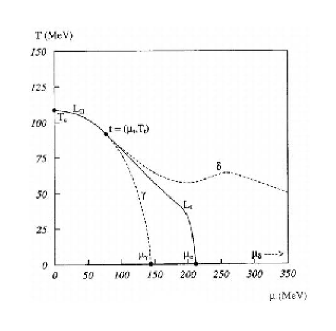
Figure 3: The continuous lines $L_{I}$ and $L_{II}$ correspond to the first and second order transitions respectively. The dot is the tricritical point, designed as $(\mu_{t},T_{t})$. The dashed lines $\gamma$ and $\delta$ (spinodal lines) are explained in the text.

At $T=\mu=0$, $g(T,\mu)$ is the QCD gauge coupling. The dependence of $g$ on $T$ and $\mu$ was chosen in a way consistent with asymptotic freedom [16]. At $T=\mu=0$ the parameters were chosen to be $\Lambda=282~{}MeV$, $\alpha_{s}=0.902$. In this way $\langle\bar{\psi}\psi\rangle$, renormalized at the scale $\Lambda$, turns out to be $(-197~{}MeV)^{3}$. The results of this analysis are shown in Fig. 3. The lines denoted by $L_{I}$ and $L_{II}$ correspond to first-order and second-order transitions (in these papers the massless quark case was considered). These two lines are separated by the critical end point (a tricritical point in this case). The dashed line $\gamma$ is the continuation of the points where the second derivative vanishes at the minimum, whereas the line $\delta$ is the location of the points where the minima of the potential go from three to one (see also Fig. 4). These two lines are called spinodal lines. The regions between $\gamma$ and $L_{I}$ and $L_{I}$ and $\delta$ correspond to metastable states. We see that the qualitative results are very similar to the ones obtained in [15] for a completely different model. Since the tricritical point is where second order and first order transitions meet together, one can perform a Ginzburg-Landau expansion of the effective potential. This was done in [19]. By performing the expansion up to $6^{th}$ order in the condensate $\chi$ one gets

$$V(\chi,T,\mu)=V(0,T,\mu)+a_{2}(T,\mu)\chi^{2}+a_{4}(T,\mu)\chi^{4}+a_{6}(T,\mu)\chi^{6}$$ (17)

The coefficients $a_{i}(\chi,T)$ have been evaluated in [19]. From this expression one easily derives the phase diagram in the plane $(a_{2}/a_{6},a_{4}/a_{6})$. In fact, it turns out that $a_{6}$ is a positive definite quantity in the region around the critical point. The resulting phase diagram is illustrated in Fig. 4 (see ref. [20]).

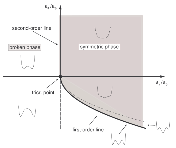
Figure 4: The phase diagram arising form the Ginzburg-Landau expansion of the effective potential. The two dashed lines correspond to the dashed lines $\gamma$ and $\delta$ of the previous figure. In particular, the line $a_{2}=0,~{}a_{4}\leq 0$ corresponds to the line $\gamma$. The shape of the effective potential in the various regions is shown in the figure.

The phase diagram of Fig. 3 is obtained from this one by mapping the plane $(a_{2}/a_{6},a_{4}/a_{6})$ into the plane $(\mu,T)$, at least in the neighborhood of the tricritical point. The second order line corresponds to $a_{2}=0$ and $a_{4}>0$, whereas the tricritical point is located at $a_{2}=a_{4}=0$. We see clearly from Fig. 4 the presence of the metastable regions. By using this approach it is possible to evaluate the critical exponents around the tricritical point. In fact, when close to it we can write

$$a_{i}(T,\mu)\approx a_{iT}\left|\frac{T-T_{c}}{T_{c}}\right|+a_{i\mu}\left|\frac{\mu-\mu_{c}}{\mu_{c}}\right|,~{}~{}~{}i=2,4$$ (18)

Let us introduce a quark mass term which, in this variables, is proportional to the field $\chi$, say

$$V_{m}=-h\chi$$ (19)

Then the minimum condition becomes

$$h=2a_{2}\chi+4a_{4}\chi^{3}+6a_{6}\chi^{5}$$ (20)

and denoting by $\theta$ either $\mu$ or $T$ one gets [19]

$$\langle\chi\rangle_{m_{q}=0,\,\theta\to\theta_{c}} \approx \left|1-\frac{\theta}{\theta_{c}}\right|^{1/4}\rightarrow\beta=\frac{1}{4}$$ (21)

$$\langle\chi\rangle_{m_{q}\to 0,\,\theta=\theta_{c}} \approx m_{q}^{1/5}\rightarrow\delta=\frac{1}{5}$$ (22)

$$\frac{\partial\langle\chi\rangle}{\partial m_{q}}_{m_{q}=0,\,\theta\to\theta_{c}} \approx \left|1-\frac{\theta}{\theta_{c}}\right|^{-1}\rightarrow\gamma=1$$ (23)

where $\alpha$, $\beta$ and $\gamma$ are the usual critical exponents. Using these relations and the scaling relations for a three-dimensional system (since the finite temperature cutoff the time-like modes):

$$\alpha=2-3\nu,~{}~{}\beta=\frac{\nu}{2}(1+\eta),~{}~{}~{}\gamma=(2-\eta)\nu,~{}~{}~{}\delta=\frac{5-\eta}{1+\eta}$$ (24)

one gets

$$\alpha=\frac{1}{2},~{}~{}~{}\nu=\frac{1}{2},~{}~{}~{}\eta=0$$ (25)

The coefficients $\alpha$, $\eta$ and $\nu$ define the behavior of the specific heat, $C(\theta)$, of the correlation length, $\xi(\theta)$, and of the correlation function at zero momentum, $G(k\to 0)$

$$C(\theta) \approx \left|1-\frac{\theta}{\theta_{c}}\right|^{-\alpha}=\left|1-\frac{\theta}{\theta_{c}}\right|^{-1/2}$$ (26)

$$\xi(\theta) \approx \left|1-\frac{\theta}{\theta_{c}}\right|^{-\nu}=\left|1-\frac{\theta}{\theta_{c}}\right|^{-1/2}$$ (27)

$$G_{\alpha\beta}(k\to 0)\approx k^{-2+\eta}=k^{-2}$$ (28)

In 1990 when we got these results we discovered a paper by Wolff [21] showing that the two-dimensional Gross-Neveu (GN) model has exactly the same phase structure found by us [16]. This was really interesting in view of the many similarities of the GN model with QCD. This convinced us that, at least qualitatively, the approximations done in our calculations did not destroy the main properties of QCD. Also the phase diagram with a tricritical point occurs in many physical systems. For instance, in the vapor-liquid transition. However, in this case the diagram usually plotted is in the variables (density, pressure) or (volume, pressure). What happens is that the degenerate minima of the first order line correspond to different densities and the line $L_{I}$ splits into two different lines. This is shown in the (density, pressure) plane in Fig. 5 (see, for instance, ref. [22]).

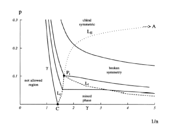
Figure 5: The phase diagram for ladder QCD (the same as for the vapor-liquid or for the GN model) in the plane $(1/n,p)$.

4 Order of the transition at zero density vs. the strange quark mass

In 1984 Pisarski and Wilczek [23] started to investigate the order of the transition at zero density. In particular they investigated the dependence of the order on the number of flavors. They used an effective theory of QCD based on the introduction of light fields transforming as the chiral condensate:

$$\Phi\approx\bar{\psi}_{L}\psi_{R}$$ (29)

When close to the transition, this is a light field since the condensate, and therefore the mass term for $\Phi$, vanishes at $T=T_{c}$. The transformation properties of $\Phi$ under the group $G=U(1)_{A}\otimes SU(N)_{L}\otimes SU(N)_{R}$ are

$$\Phi\to e^{i\alpha}U_{L}\Phi U_{R}\,,~{}~{}~{}U_{L}\in SU(N)_{L}\,,~{}U_{R}\in SU(N)_{R}$$ (30)

It is convenient to parameterize $\Phi$ in the form

$$\Phi=\phi U,~{}~{}~{}U\in SU(N)$$ (31)

In this way we separate the $N^{2}-1$ Goldstone fields from the condensate $\phi$. The effective G-invariant lagrangian is [23]

$${\cal L}=\frac{1}{2}{\rm tr}\,(\partial_{\mu}\Phi^{\dagger}\partial^{\mu}\Phi)-\frac{1}{2}m^{2}{\rm tr}\,(\Phi^{\dagger}\Phi)-g_{1}\left(tr\,(\Phi^{\dagger}\Phi)\right)^{2}-g_{2}{\rm tr}\,(\Phi^{\dagger}\Phi)^{2}$$ (32)

To this G-invariant part a piece breaking $U(1)_{A}\to Z_{A}(N)$ is added

$${\cal L}^{\prime}=c\left({\rm det}\,\Phi+{\rm det}\,\Phi^{\dagger}\right)$$ (33)

At zero temperature the symmetry breaking to $SU(N)_{L+R}$ is enforced through the non vanishing expectation value

$$\langle\Phi\rangle=\Phi_{0}\cdot 1$$ (34)

In [23] the $\beta$-function of this effective theory has been studied and it was found that for $N\geq 3$ the transition to the symmetric phase is first-order. The proof goes through the use of the $\epsilon$-expansion in $4-\epsilon$ dimensions and the analytic continuation to $\epsilon=1$. In this way one takes into account that, due to the thermal cutoff of the time-like modes, the theory is effectively three dimensional. About this point notice that at $d=3$ the dimensions of the scalar fields are $[\Phi]=1/2$. As a consequence the sixth order term $\phi^{6}$ is marginal and it should be included into the effective expansion when the coefficients of $\Phi^{2}$ and $\Phi^{4}$ are small, that is around the tricritical point. At zero density and close to the critical point $T_{c}$ the effective potential for the condensate $\phi$ can be taken of of the form (see eqs. 32 and 33)

$$\frac{M^{2}}{2}\phi^{2}+\frac{\lambda}{4}\phi^{4}$$ (35)

with the coefficients $M^{2}$ and $\lambda$ depending on the parameter of the effective lagrangian $m^{2}$, $g_{1}$, $g_{2}$, $c$ and $N$. The critical temperature can then determined as a function of the parameters by the equation

$$M(T_{c})=0$$ (36)

This result was also confirmed by lattice calculations, as shown in Table 1.

Date	Authors	$N=2$	$N=3$	$N=4$	$N=6$	Lattice size
1987	Gottlieb et al. [24]	crossover		$1^{st}$		$(8,10)^{3}\times 4$
1990	Gottlieb et al. [25]	crossover				$12^{3}\times 8$
1990	Fukugita et al. [26]	crossover		$1^{st}$		$12^{3}\times 4$
1990	Kogut et al. [27]	crossover	$1^{st}$?	$1^{st}$		$12^{3}\times 4$
1990	Brown et al. [28]	crossover	$1^{st}$			$16^{3}\times 4$
1992	Bernard et al. [29]	crossover				$12^{3}\times 6$
1994	Zhu [30]	crossover				$(16,32)^{3}\times 8$
1995	Iwasaki et al. [31]	crossover	$1^{st}$		$1^{st}$	$12^{3}(6,18),18^{2}\times 24\times(6,18)$

Table 1: A compilation of the results obtained in lattice calculations of the order of the chiral transition at $\mu=0$ and $T\not=0$.

Following ref. [28] we may draw the phase diagram in the space of the quark masses as in Fig. 6.

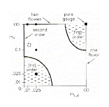
Figure 6: Solid circles is where the first order transition is seen, whereas crossover transitions correspond to the solid squares. The dashed circle indicates the physical point.

By looking at this diagram an interesting question arises: how do we go from a second order to a first order phase transition by varying the strange quark mass? An answer to this question was given in refs. [32, 33]. The argument is the following: adding a massive quark does not change the effective action since the light fields are unchanged. Therefore, when close to the critical point, the effective potential is still of the form given in eq. 35. However the massive quark renormalizes the couplings. The resulting effect is that a variation of $M^{2}$ will change the critical temperature. However $\lambda$ could change in such a way to go through zero and become negative. If this is the case we know that we have to add a $\phi^{6}$ term in the potential (remember that the effective theory is three dimensional and that such an operator is marginal). In this way we may go smoothly from a second order to a first order transition.

5 Universality at non zero density

Figure 7: Dashed lines represent second order phase transitions, whereas the solid line corresponds to a first order one. The solid circle indicates the tricritical point.

At the end of the 90’s there was a big revival of the studies of the phase diagram of QCD prompted by the analysis made at very large density and zero temperature [2], showing the formation of a diquark condensate $\langle\psi\psi\rangle$ and the corresponding breaking of the color symmetry. After that Berges and Rajagopal [34] studied the coexistence of the chiral and of the diquark condensates in a NJL model. The phase diagram found by these authors is shown in Fig. 7, and it shows the presence of the tricritical point. The authors justified the presence of the tricritical point by using an argument very close to the one used in refs. [32, 33] in the case of the strange quark that we have discussed in the previous section. The idea is that at zero quark mass the theory belongs to the O(4) universality class (Ising $Z_{2}$ for $m_{q}\not=0$) and this is not changed at finite density as shown in ref. [35]. However the renormalization of the coefficients in the effective action due to the presence of the chemical potential might change the coefficient of the quartic term forcing the introduction of a sixth order term in the potential. Again, the $6^{\,th}$ order term gives rise to a tricritical point in the phase diagram. Also, recalling that the $\phi^{6}$ operator is marginal, one expects, at most, logarithmic corrections to the critical exponents evaluated before.

After the previous paper many authors reconsidered the problem of QCD at finite density and temperature using many different approaches. We will give here a brief list of papers delaing with the problem. In 1998 Halasz et al. [36] considered a random matrix model, for the two-flavor case, in the space $(\mu,T,m)$ finding results consistent the universality arguments. Their results are shown in Fig. 8.

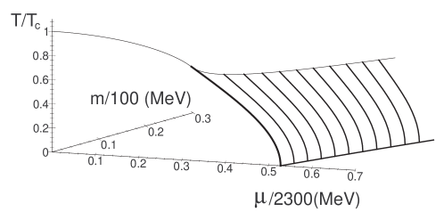
Figure 8: We show the first order lines as curves at constant quark mass, $m$. At $m=0$ the second order line is shown. For $m\not=0$ the first order line ends into a critical end point.

In ref. [37] the chiral phase transition has been examined both in a linear $\sigma$-model and in a NJL model. The two cases are illustrated in Fig. 9. Once again the results agree very well with the universality arguments.

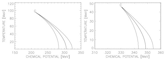
Figure 9: The two panels illustrate the phase diagram for the $\sigma$-model (left panel) and for the NJL model (right panel). The middle curves are the critical lines whereas the outer lines are the spinodal lines.

Another different approach was considered in ref. [38]. The calculation was done within the context of the statistical boostrap principle, and again it agrees with the universality hypothesis, see Fig. 10. It was also found that the critical chemical potential is non zero for a large range of values of the bag constant $B$ ($B^{1/4}<282~{}MeV$).

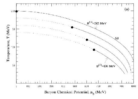
Figure 10: The $(\mu,T)$ phase diagram from the statistical boostrap model. $B$ is the value of the bag constant.

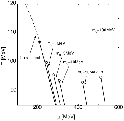
Figure 11: Quark masses are evaluated at the momentum scale 1 $GeV$. The solid and dotted lines correspond to first order and second order phase transitions respectively. The solid and open circles denotes the tricritical and the critical end points.

As a last example we report a recent calculation made by Hatta and Ikeda [39] using again ladder QCD with the help of the CJT potential as in refs. [16, 17]. This calculation takes also into account quark masses and it shows the dependence of the critical end point with this variable, as shown in Fig. 11.

A comparison of the locations of the critical end point evaluated in different models can be found in a recent review by Stephanov [5]. This comparison is particularly interesting since it shows that, although different models agree qualitatively well, from a quantitative point of view they are quite different. For instance, at the critical end point, the critical value of the chemical potential varies between roughly 300 $MeV$ up to about 1000 $MeV$, whereas the critical value of the temperature goes between 40 and 170 $MeV$. Clearly in order to have a quantitative improvement one would need a first principles calculation.

6 Lattice calculations

As noticed in the previous section one would really need to have the possibility of testing on the lattice the phase diagram of QCD. However the usual sampling method, based on a positive definite measure in the euclidean path integral, does not work in presence of a real chemical potential, since the fermionic determinant is then complex. In fact, let us define euclidean variables through the following substitutions:

$$x_{0}\to-ix_{E}^{4},~{}~{}x^{i}\to x^{i}_{E},~{}~{}\gamma_{0}\to\gamma_{E}^{4},~{}~{}\gamma^{i}\to-i\gamma_{E}^{i}$$ (37)

The euclidean Dirac operator in the presence of a chemical potential is

$$D(\mu)=\gamma^{\mu}_{E}D^{\mu}_{E}+\mu\gamma_{E}^{4},~{}~{}~{}D^{\mu}_{E}=\partial_{E}^{\mu}+iA_{E}^{\mu}$$ (38)

At $\mu=0$ the eigenvalues of $D(\mu)$ are pure imaginary and also, if $|\lambda\rangle$ is an eigenvector of $D(0)$, then $\gamma_{5}|\lambda\rangle$ belongs to the eigenvalue $-\lambda_{5}$, as it follows from

$$D(0)^{\dagger}=-D(0),~{}~{}~{}\gamma_{5}D(0)\gamma_{5}=-D(0)$$ (39)

Therefore

$${\rm det}[D(0)]=\prod_{\lambda}(\lambda)(-\lambda)>0$$ (40)

At $\mu\not=0$ this argument does not hold and we lack the positivity property. However, if one considers the chemical potential associated to the isospin, since this is related to the conserved current $\tau_{3}$, the positivity can be proved by using $\tau_{1}$ in conjunction with the hermitian conjugation.

Recently there have been numerous different attempts to improve the lattice calculations at $\mu\not=0$:

• Rewighting method (see, for instance [40, 41, 42]).

• Taylor expansion for small $\mu$ (see, for instance [43], [44], [45])

• Imaginary chemical potential (see, for example [46], [47] [48], [49], [50])

6.1 Reweighting

The reweighting technique (for a review see ref. [51])is based on the following identity for the partition function

$$\int D\,U{\rm det}\,[D(0)]\frac{{\rm det}\,[D(\mu)]}{{\rm det}\,[D(0)]}e^{-S_{g}(U)}=\left\langle\frac{{\rm det}\,[D(\mu)]}{{\rm det}\,[D(0)]}\right\rangle_{\mu=0}$$ (41)

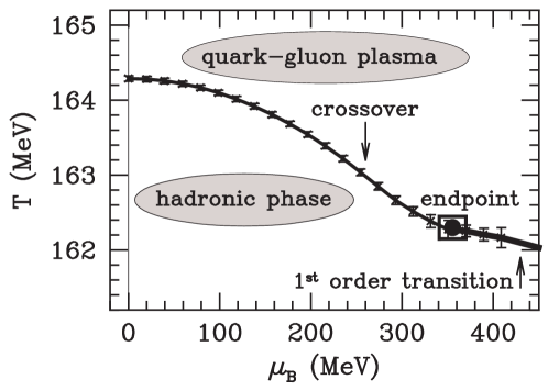
Figure 12: The most recent determination with the reweighting procedure is given in ref. [42]. The errors are due to the reweighting procedure and on the error of the scale determination at $T=0$. The values of the critical temperature and chemical potential are $T=162\pm 2~{}MeV$, $\mu=360\pm 40~{}MeV$.

Since the integration measure is taken at $\mu=0$ it is positive definite. However in the numerical calculation problems arise. The ratio of the two determinants oscillates and there are large cancellations. Also, since the reweighting corresponds to the ratio of two partition functions with different actions, it decays exponentially according to the difference of the free energies, $\Delta F$. This is proportional to the volume and therefore the statistics required for a given accuracy increases with the volume. An improvement of this technique is the so called ”multiparameter reweighting” which is a generalization of the previous method [40]. The idea is to reweight also in the lattice gauge coupling, writing

$$Z=\left\langle\frac{e^{-S_{g}(\beta)}{\rm det}\,[D(\mu)]}{e^{-S_{g}(\beta_{0})}{\rm det}\,[D(0)]}\right\rangle_{\mu=0,\beta_{0}}$$ (42)

The second reweighting parameter can be used to allow the statistical ensemble to fluctuate between the phases and to avoid that the ensemble goes away from criticality. One of the most recent calculations using this technique was done in ref. [42] and the result is shown in Fig. 12

6.2 Taylor expansion

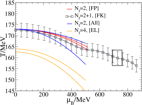
Figure 13: A comparison of the critical line in different simulations, FP [48], FK [41], All [43], EL [47]. The box is the position of the critical end point evaluated by Fodor and Katz in [41].

This method makes use of the multiparameter reweighting and at the same time of a Taylor expansion in the chemical potential. Although this method is not useful for determining the critical end point, it is of interest in the heavy ion physics where values of $\mu$ of a few ten $MeV$ are important. What one does is simply to expand in a Taylor series of $\mu/T$ the reweighting factor. In particular this method can be used to evaluate the behavior of the critical line at small $\mu/T$. This method has been used in ref. [43] for the two-flavor case. The results are shown in Fig. 13.

6.3 Imaginary chemical potential

If $\mu$ is pure imaginary the fermion determinant is positive and numerical simulations can be done easily as for the case $\mu=0$. Using the fact that the observables are analytic functions of $\mu$ except that on the critical line, one computes expectation values at imaginary $\mu$ and then one fits them by a truncated Taylor expansion [46, 47]. Some of these results are given in Fig. 13.

7 Isospin chemical potential

To end this review we will report also some result obtained in presence of an isospin chemical potential, $\mu_{I}$. The case of $\mu_{I}\not=0$ is, in principle, interesting for the heavy ion physics. It is also interesting since for $\mu=0$ and $\mu_{I}\not=0$ the fermionic determinant is positive [52, 53]. The problem ($\mu$ and $\mu_{I}\not=0$) has been studied using effective lagrangians [54, 55], random matrices [56], NJL model [57, 58] and ladder-QCD [59]. The most interesting effect in these studies appears to be the splitting of the critical line and of the critical end point. In fact, this effect could bring down the end critical point to a region more accessible to heavy ion experiments. We show in Fig. 14 the result in the NJL model [57]. The result is qualitatively compatible with an analogous calculation made in the ladder-QCD model [59]. However a too strong mixing of the up and down flavors could destroy this interesting result, as shown in ref. [60].

Figure 14: The phase diagram for the NJL model as studied in ref. [57]. The left panel shows the case $\mu_{I}=0$, whereas in the right panel $\mu_{I}=30~{}MeV$.

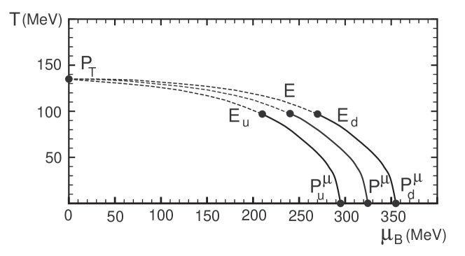
Figure 15: The phase diagram for the ladder-QCD model as studied in ref. [59].

8 Conclusions

As we have shown there has been a lot of activities and results in our understanding of the phase diagram of QCD. However most of the progress is still at a very qualitative level. We would like to be able to locate the critical point with a good accuracy, but for that, a breakthrough is real necessary. This could come by devising some clever technique in lattice calculations, or, may be, a new analytical method.

References

- [1] B. Barrois, Nuclear Physics B129, 390 (1977); S. Frautschi, Proceedings of workshop on hadronic matter at extreme density, Erice 1978; D. Bailin and A. Love, Physics Report 107 (1984) 325 .
- [2] M. Alford, K. Rajagopal, and F. Wilczek, Phys. Lett. B422(1998) 247 [hep-ph/9711395]; R. Rapp, T. Schafer, E. V. Shuryak and M. Velkovsky, Phys. Rev. Lett. 81, 53 (1998) [hep-ph/9711396].
- [3] K. Rajagopal, arXiv:hep-ph/9504310.
- [4] K. Rajagopal and F. Wilczek, arXiv:hep-ph/0011333.
- [5] M. A. Stephanov, Prog. Theor. Phys. Suppl. 153 (2004) 139 [Int. J. Mod. Phys. A 20 (2005) 4387] [arXiv:hep-ph/0402115].
- [6] H. Satz, Int. J. Mod. Phys. A 21 (2006) 672 [arXiv:hep-lat/0509192].
- [7] T. Schafer, arXiv:hep-ph/0509068.
- [8] L. D. McLerran and B. Svetitsky, Phys. Lett. B 98 (1981) 195; L. D. McLerran and B. Svetitsky, Phys. Rev. D 24 (1981) 450; J. Kuti, J. Polonyi and K. Szlachanyi, Phys. Lett. B 98, 199 (1981).
- [9] F. Karsch and E. Laermann, Phys. Rev. D 50 (1994) 6954 [arXiv:hep-lat/9406008].
- [10] D. Bailin, J. Cleymans and M. D. Scadron, Phys. Rev. D 31 (1985) 164.
- [11] A. Kocic, Phys. Rev. D 33 (1986) 1785.
- [12] V. F. Galina and K. S. Viswanathan, Phys. Rev. D 38 (1988) 2000.
- [13] P. H. Damgaard, D. Hochberg and N. Kawamoto, Phys. Lett. B 158 (1985) 239.
- [14] E. M. Ilgenfritz and J. Kripfganz, Z. Phys. C 29 (1985) 79.
- [15] M. Asakawa and K. Yazaki, Nucl. Phys. A 504 (1989) 668.
- [16] A. Barducci, R. Casalbuoni, S. De Curtis, R. Gatto and G. Pettini, Phys. Lett. B 231 (1989) 463.
- [17] A. Barducci, R. Casalbuoni, S. De Curtis, R. Gatto and G. Pettini, Phys. Rev. D 41 (1990) 1610.
- [18] J. M. Cornwall, R. Jackiw and E. Tomboulis, Phys. Rev. D 10, 2428 (1974).
- [19] A. Barducci, R. Casalbuoni, S. De Curtis, R. Gatto and G. Pettini, Phys. Rev. D 42 (1990) 1757.
- [20] A. Barducci, R. Casalbuoni, S. De Curtis, R. Gatto and G. Pettini, UGVA-DPT-1990-10-697, Proceedings of the Large hadron collider workshop, Aachen, Germany, Oct 4-9, 1990, edited by G. Jarlskog and D. Rein. Geneva, Switzerland, CERN, 1990. 3 volumes. (CERN-90-10)
- [21] U. Wolff, Phys. Lett. B 157 (1985) 303.
- [22] A. Barducci, R. Casalbuoni, M. Modugno, G. Pettini and R. Gatto, Phys. Rev. D 51 (1995) 3042 [arXiv:hep-th/9406117].
- [23] R. D. Pisarski and F. Wilczek, Phys. Rev. D 29 (1984) 338.
- [24] S. A. Gottlieb, W. Liu, D. Toussaint, R. L. Renken and R. L. Sugar, Nucl. Phys. Proc. Suppl. 4 (1988) 155.
- [25] S. A. Gottlieb, W. Liu, R. L. Renken, R. L. Sugar and D. Toussaint, Phys. Rev. D 41 (1990) 622.
- [26] M. Fukugita, H. Mino, M. Okawa and A. Ukawa, Phys. Rev. Lett. 65 (1990) 816.
- [27] J. B. Kogut and D. K. Sinclair, Nucl. Phys. B 344 (1990) 238.
- [28] F. R. Brown et al., Phys. Rev. Lett. 65 (1990) 2491.
- [29] C. W. Bernard et al., Phys. Rev. D 45 (1992) 3854.
- [30] D. c. Zhu, Numerical Study Of Two-Flavor QCD Phase Structures At N(T) = 8 On 16**3 And 32**3 Volumes, PhD thesis, UMI-95-16217
- [31] Y. Iwasaki, K. Kanaya, S. Sakai and T. Yoshie, Z. Phys. C 71 (1996) 337 [arXiv:hep-lat/9504019].
- [32] F. Wilczek, Int. J. Mod. Phys. A 7 (1992) 3911 [Erratum-ibid. A 7 (1992) 6951].
- [33] K. Rajagopal and F. Wilczek, Nucl. Phys. B 399 (1993) 395 [arXiv:hep-ph/9210253].
- [34] J. Berges and K. Rajagopal, Nucl. Phys. B 538 (1999) 215 [arXiv:hep-ph/9804233].
- [35] S. D. H. Hsu and M. Schwetz, Phys. Lett. B 432 (1998) 203 [arXiv:hep-ph/9803386].
- [36] M. A. Halasz, A. D. Jackson, R. E. Shrock, M. A. Stephanov and J. J. M. Verbaarschot, Phys. Rev. D 58 (1998) 096007 [arXiv:hep-ph/9804290].
- [37] O. Scavenius, A. Mocsy, I. N. Mishustin and D. H. Rischke, Phys. Rev. C 64 (2001) 045202 [arXiv:nucl-th/0007030].
- [38] N. G. Antoniou and A. S. Kapoyannis, Phys. Lett. B 563 (2003) 165 [arXiv:hep-ph/0211392].
- [39] Y. Hatta and T. Ikeda, Phys. Rev. D 67 (2003) 014028 [arXiv:hep-ph/0210284].
- [40] Z. Fodor and S. D. Katz, Phys. Lett. B 534 (2002) 87 [arXiv:hep-lat/0104001].
- [41] Z. Fodor and S. D. Katz, JHEP 0203 (2002) 014 [arXiv:hep-lat/0106002].
- [42] Z. Fodor and S. D. Katz, JHEP 0404 (2004) 050 [arXiv:hep-lat/0402006].
- [43] C. R. Allton et al., Phys. Rev. D 66 (2002) 074507 [arXiv:hep-lat/0204010].
- [44] C. R. Allton, S. Ejiri, S. J. Hands, O. Kaczmarek, F. Karsch, E. Laermann and C. Schmidt, Phys. Rev. D 68 (2003) 014507 [arXiv:hep-lat/0305007].
- [45] S. Ejiri, C. R. Allton, S. J. Hands, O. Kaczmarek, F. Karsch, E. Laermann and C. Schmidt, Prog. Theor. Phys. Suppl. 153 (2004) 118 [arXiv:hep-lat/0312006].
- [46] M. P. Lombardo, Nucl. Phys. Proc. Suppl. 83 (2000) 375 [arXiv:hep-lat/9908006].
- [47] M. D’Elia and M. P. Lombardo, Phys. Rev. D 67 (2003) 014505 [arXiv:hep-lat/0209146].
- [48] P. de Forcrand and O. Philipsen, Nucl. Phys. B 642 (2002) 290 [arXiv:hep-lat/0205016].
- [49] P. de Forcrand and O. Philipsen, Nucl. Phys. B 673 (2003) 170 [arXiv:hep-lat/0307020].
- [50] M. A. Stephanov, Phys. Rev. D 73 (2006) 094508 [arXiv:hep-lat/0603014].
- [51] I. M. Barbour, S. E. Morrison and J. B. Kogut [UKQCD Collaboration], Nucl. Phys. Proc. Suppl. 63 (1998) 436 [arXiv:hep-lat/9612012].
- [52] J. B. Kogut and D. K. Sinclair, Phys. Rev. D 66 (2002) 034505 [arXiv:hep-lat/0202028].
- [53] S. Gupta, arXiv:hep-lat/0202005.
- [54] D. T. Son and M. A. Stephanov, Phys. Rev. Lett. 86, 592 (2001) [arXiv:hep-ph/0005225].
- [55] M. Loewe and C. Villavicencio, Phys. Rev. D 67 (2003) 074034 [arXiv:hep-ph/0212275].
- [56] B. Klein, D. Toublan and J. J. M. Verbaarschot, Phys. Rev. D 68 (2003) 014009 [arXiv:hep-ph/0301143].
- [57] D. Toublan and J. B. Kogut, Phys. Lett. B 564 (2003) 212 [arXiv:hep-ph/0301183].
- [58] A. Barducci, R. Casalbuoni, G. Pettini and L. Ravagli, Phys. Rev. D 69 (2004) 096004 [arXiv:hep-ph/0402104].
- [59] A. Barducci, G. Pettini, L. Ravagli and R. Casalbuoni, Phys. Lett. B 564 (2003) 217 [arXiv:hep-ph/0304019].
- [60] M. Frank, M. Buballa and M. Oertel, Phys. Lett. B 562 (2003) 221 [arXiv:hep-ph/0303109].