hep-ph/*** DFPD-06/TH/12

RM3-TH/06-17

CERN-PH-TH/2006-205

Tri-bimaximal Neutrino Mixing from Orbifolding

Guido Altarelli 

Dipartimento di Fisica ‘E. Amaldi’, Università di Roma Tre

INFN, Sezione di Roma Tre, I-00146 Rome, Italy

and

CERN, Department of Physics, Theory Division

CH-1211 Geneva 23, Switzerland

Ferruccio Feruglio  and Yin Lin 

Dipartimento di Fisica ‘G. Galilei’, Università di Padova

INFN, Sezione di Padova, Via Marzolo 8, I-35131 Padua, Italy

We show that the $A_{4}$ discrete symmetry that naturally leads to tri-bimaximal neutrino mixing can be simply obtained as a result of an orbifolding starting from a model in 6 dimensions. This particular orbifolding has four fixed points where 4 dimensional branes are located and the tetrahedral symmetry of $A_{4}$ connects these branes. In this approach $A_{4}$ appears after the reduction from six to four dimensions as a remnant of the 6D space-time symmetry. A previously discussed supersymmetric version of $A_{4}$ is reinterpreted along these lines.

1 Introduction

It is an experimental fact [1] that within measurement errors the observed neutrino mixing matrix is compatible with the so called tri-bimaximal form, introduced by Harrison, Perkins and Scott (HPS) [2]. It is an interesting challenge to formulate dynamical principles that, in a completely natural way, can lead to this specific mixing pattern as a first approximation, with small corrections determined by higher order terms in a well defined expansion. In a series of papers [3, 4] it has been pointed out that a broken flavour symmetry based on the discrete group $A_{4}$ appears to be particularly fit for this purpose. Other solutions based on continuous flavour groups like SU(3) or SO(3) have also been recently presented [5, 6], but the $A_{4}$ models have a very economical and attractive structure (for example, in terms of field content). A crucial feature of all HPS models is the mechanism used to guarantee the necessary VEV alignment of the flavon field $\varphi_{T}$ which determines the charged lepton mass matrix with respect to the direction in flavour space chosen by the flavon $\varphi_{S}$ that gives the neutrino mass matrix. In recent papers [7, 8] we have constructed explicit versions of $A_{4}$ model where the alignment problem is solved. In ref. [7] we adopted an extra dimensional framework, with $\varphi_{T}$ and $\varphi_{S}$ on different branes so that the minimization of the respective potentials is kept to a large extent independent. In ref. [8], we presented an alternative, perhaps more conventional, formulation of the $A_{4}$ model in 4 dimensions with supersymmetry (SUSY) at the price of introducing a somewhat less economic set of fields. Versions either with see-saw or without see-saw can be constructed. The existence of different realizations shows that the connection of $A_{4}$ with the HPS matrix is robust and does not necessarily require extra dimensions.

Another important aspect of the problem is that of trying to understand the dynamical origin of $A_{4}$. As a first move in this direction, in ref. [8] we have reformulated $A_{4}$ as a subgroup of the modular group which often plays a role in the formalism of string theories, for example in the context of duality transformations [9]. In the present note we show that the $A_{4}$ symmetry can be simply obtained by orbifolding starting with a model in 6 dimensions (6D). In this approach $A_{4}$ appears as the remnant of the reduction from 6D to 4D space-time symmetry induced by the special orbifolding adopted. There are 4D branes at the four fixed points of the orbifolding and the tetrahedral symmetry of $A_{4}$ connects these branes. The standard model fields have components on the fixed point branes while the scalar fields necessary for the $A_{4}$ breaking are in the bulk.

In this paper, starting from a 6D field theory, we first introduce the specific orbifolding with four fixed points on which the 4D standard model fields live (while a number of additional gauge singlets are in the bulk) and specify how the $A_{4}$ transformations relate the field components on different branes or on the bulk. We then study the invariant interactions, local in 6D, constructed out of the fields in the theory which are invariant under $A_{4}$. Finally we rederive the SUSY model for tri-bimaximal neutrino mixing in this particular framework.

2 $A_{4}$ as the isometry of $T^{2}/Z_{2}$

We consider a quantum field theory in 6 dimensions, with two extra dimensions compactified on an orbifold $T^{2}/Z_{2}$. We denote by $z=x_{5}+ix_{6}$ the complex coordinate describing the extra space. The torus $T^{2}$ is defined by identifying in the complex plane the points related by

$$\begin{array}[]{l}z\to z+1\\ z\to z+\gamma~{}~{}~{}~{}~{}~{}~{}~{}~{}~{}~{}~{}~{}~{}~{}~{}~{}\gamma=e^{\displaystyle i\frac{\pi}{3}}~{}~{}~{},\end{array}$$ (1)

where our length unit, $2\pi R$, has been set to 1 for the time being. The parity $Z_{2}$ is defined by

$$z\to-z$$ (2)

and the orbifold $T^{2}/Z_{2}$ can be represented by the fundamental region given by the triangle with vertices $0,1,\gamma$, see Fig. 1. The orbifold has four fixed points, $(z_{1},z_{2},z_{3},z_{4})=(1/2,(1+\gamma)/2,\gamma/2,0)$. The fixed point $z_{4}$ is also represented by the vertices $1$ and $\gamma$. In the orbifold, the segments labelled by $a$ in Fig. 1, $(0,1/2)$ and $(1,1/2)$, are identified and similarly for those labelled by $b$, $(1,(1+\gamma)/2)$ and $(\gamma,(1+\gamma)/2)$, and those labelled by $c$, $(0,\gamma/2)$, $(\gamma,\gamma/2)$. Therefore the orbifold is a regular tetrahedron with vertices at the four fixed points.

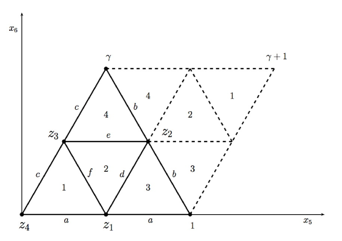
Figure 1: Orbifold $T_{2}/Z_{2}$. The regions with the same numbers are identified with each other. The four triangles bounded by solid lines form the fundamental region, where also the edges with the same letters are identified. The orbifold $T_{2}/Z_{2}$ is exactly a regular tetrahedron with 6 edges $a,b,c,d,e,f$ and four vertices $z_{1}$, $z_{2}$, $z_{3}$, $z_{4}$, corresponding to the four fixed points of the orbifold.

The symmetry of the uncompactified 6D space time is broken by compactification. Here we assume that, before compactification, the space-time symmetry coincides with the product of 6D translations and 6D proper Lorentz transformations. The compactification breaks part of this symmetry. However, due to the special geometry of our orbifold, a discrete subgroup of rotations and translations in the extra space is left unbroken. This group can be generated by two transformations:

$$\begin{array}[]{ll}{\cal S}:&z\to z+\frac{1}{2}\\ {\cal T}:&z\to\omega z~{}~{}~{}~{}~{}~{}~{}~{}~{}~{}~{}~{}~{}\omega\equiv\gamma^{2}~{}~{}~{}~{}.\end{array}$$ (3)

Indeed ${\cal S}$ and ${\cal T}$ induce even permutations of the four fixed points:

$$\begin{array}[]{cc}{\cal S}:&(z_{1},z_{2},z_{3},z_{4})\to(z_{4},z_{3},z_{2},z_{1})\\ {\cal T}:&(z_{1},z_{2},z_{3},z_{4})\to(z_{2},z_{3},z_{1},z_{4})\end{array}~{}~{}~{},$$ (4)

thus generating the group $A_{4}$. From the previous equations we immediately verify that ${\cal S}$ and ${\cal T}$ satisfy the characteristic relations obeyed by the generators of $A_{4}$:

$${\cal S}^{2}={\cal T}^{3}=({\cal ST})^{3}=1~{}~{}~{}.$$ (6)

These relations are actually satisfied not only at the fixed points, but on the whole orbifold, as can be easily checked from the general definitions of ${\cal S}$ and ${\cal T}$ in eq. (3), with the help of the orbifold defining rules in eqs. (1) and (2). In our model the discrete group $A_{4}$, together with 4D translations and 4D proper Lorentz transformations, can be seen as the subgroup of the space-time symmetry in six dimensions that survives compactification. In a similar context, the compactification of two extra dimensions on an orbifold $T^{2}/Z_{3}$ and its relation to the flavour symmetry $Z_{3}$ has been analyzed in ref. ([10]).

It is useful to represent the action of ${\cal S}$ and ${\cal T}$ on the fixed points by means of the four by four matrices $S$ and $T^{-1}$ respectively.

$$S=\left(\begin{array}[]{cccc}0&0&0&1\\ 0&0&1&0\\ 0&1&0&0\\ 1&0&0&0\end{array}\right)~{}~{}~{},~{}~{}~{}~{}~{}~{}~{}~{}~{}~{}T^{-1}=\left(\begin{array}[]{cccc}0&1&0&0\\ 0&0&1&0\\ 1&0&0&0\\ 0&0&0&1\end{array}\right)~{}~{}~{}.$$ (7)

The matrices $S$ and $T$ satisfy the relations (6), thus providing a representation of $A_{4}$. Since the only irreducible representations of $A_{4}$ are a triplet and three singlets, the 4D representation described by $S$ and $T$ is not irreducible. It decomposes into the sum of the invariant singlet plus the triplet representation. If we denote by $u=(u_{1},u_{2},u_{3},u_{4})^{t}$ (the suffix $t$ denotes transposition) a multiplet transforming as

$$u\to Su~{}~{}~{},~{}~{}~{}~{}~{}~{}~{}u\to Tu~{}~{}~{},$$ (8)

under $S$ and $T$ respectively, then singlet corresponds to

$$u_{1}=u_{2}=u_{3}=u_{4}~{}~{}~{},$$ (9)

while the triplet is obtained by imposing the constraint

$$\sum_{i=1}^{4}u_{i}=0~{}~{}~{}.$$ (10)

Both conditions (9) and (10) are invariant under $A_{4}$. To better visualize this decomposition, we consider the unitary matrix $U$ given by:

$$U=\frac{1}{2}\left(\begin{array}[]{cccc}+1&+1&+1&+1\\ &&&\\ -1&+1&+1&-1\\ &&&\\ +1&-1&+1&-1\\ &&&\\ +1&+1&-1&-1\end{array}\right)~{}~{}~{}.$$ (11)

This matrix maps $S$ and $T$ into matrices that are block-diagonal:

$$USU^{\dagger}=\left(\begin{array}[]{c|ccc}1&&0&\\ \hline\cr&&&\\ 0&&S_{3}&\\ &&&\end{array}\right)~{}~{}~{},~{}~{}~{}~{}~{}~{}~{}~{}~{}~{}UTU^{\dagger}=\left(\begin{array}[]{c|ccc}1&&0&\\ \hline\cr&&&\\ 0&&T_{3}&\\ &&&\end{array}\right)~{}~{}~{},$$ (12)

where $S_{3}$ and $T_{3}$ are the generators of the three-dimensional representation:

$$S_{3}=\left(\begin{array}[]{ccc}1&0&0\\ 0&-1&0\\ 0&0&-1\end{array}\right)~{}~{}~{},~{}~{}~{}~{}~{}~{}~{}~{}~{}~{}T_{3}=\left(\begin{array}[]{ccc}0&0&1\\ 1&0&0\\ 0&1&0\end{array}\right)~{}~{}~{}.$$ (13)

If $u=(u_{1},u_{2},u_{3},u_{4})^{t}$ transforms as specified in eq. (8), then $v\equiv(v_{0},v_{1},v_{2},v_{3})^{t}=Uu$ transforms as

$$v\to(USU^{\dagger})v~{}~{}~{},~{}~{}~{}~{}~{}~{}~{}v\to(UTU^{\dagger})v~{}~{}~{},$$ (14)

respectively. Therefore, if we parametrize $u$ as

$$\left(\begin{array}[]{c}u_{1}\\ u_{2}\\ u_{3}\\ u_{4}\end{array}\right)=\displaystyle\frac{1}{2}\left(\begin{array}[]{c}v_{0}\\ v_{0}\\ v_{0}\\ v_{0}\end{array}\right)+\displaystyle\frac{1}{2}\left(\begin{array}[]{c}-v_{1}+v_{2}+v_{3}\\ +v_{1}-v_{2}+v_{3}\\ +v_{1}+v_{2}-v_{3}\\ -v_{1}-v_{2}-v_{3}\end{array}\right)~{}~{}~{},$$ (15)

the components $(v_{1},v_{2},v_{3})^{t}$ transform with $S_{3}$ and $T_{3}$, whereas the component $v_{0}$ is left invariant by $A_{4}$. It is useful to observe that $v_{0}$ is given by $v_{0}=(u_{1}+u_{2}+u_{3}+u_{4})/2$ while the sum of all components of the last multiplet in eq. (15) vanishes, in agreement with the conditions (9) and (10). Finally, if we restrict to the case of a pure triplet by taking $v_{0}=0$, then $v_{1}$, $v_{2}$ and $v_{3}$ are given by:

$$\left(\begin{array}[]{c}0\\ v_{1}\\ v_{2}\\ v_{3}\end{array}\right)=U\left(\begin{array}[]{c}u_{1}\\ u_{2}\\ u_{3}\\ -u_{1}-u_{2}-u_{3}\end{array}\right)=\left(\begin{array}[]{c}0\\ u_{2}+u_{3}\\ u_{1}+u_{3}\\ u_{1}+u_{2}\end{array}\right)~{}~{}~{}.$$ (16)

3 Local interactions invariant under $A_{4}$

In this section we collect the rules to construct an $A_{4}$ invariant field theory in the 6D space-time ${\cal M}\times T^{2}/Z_{2}$. The fields of this theory can be either 4D fields living at the fixed points, in short ‘brane’ fields, or ‘bulk’ fields depending on both the uncompactified coordinates $x$ and the complex coordinate $z$. The new essential feature with respect to a 4D formalism is that in general all particles have components over all four fixed points. Locality in 6D implies that at each fixed point only products of components on that brane are allowed in the interaction terms. This constraint reduces the number of invariant interactions that can be constructed out of brane fields. We now discuss the structure of the invariants in this context.

3.1 Brane fields

We first consider the case of brane fields and we denote by

$$a=(a_{1}(x),a_{2}(x),a_{3}(x),a_{4}(x))$$ (17)

a set of fields localized at the fixed points $(z_{1},z_{2},z_{3},z_{4})$, respectively. For the time being we do not specify if $a$ is a scalar, a spinor or a vector under the 4D Lorentz group. We denote by $\delta_{i}=\delta(z-z_{i})$ the 2D Dirac deltas needed to construct an interaction term local in 6D, starting from brane fields. We observe that, if $z$ undergoes the transformations (3), then the delta functions $\delta=(\delta_{1},\delta_{2},\delta_{3},\delta_{4})^{t}$ are mapped into

$$\begin{array}[]{cc}{\cal S}:&\delta\to S\delta\\ {\cal T}:&\delta\to T\delta\end{array}~{}~{}~{},$$ (18)

where $S$ and $T$ are given in eq. (7). The $A_{4}$ transformations of $a$ are naturally given by:

$$\begin{array}[]{cl}{\cal S}:&a\to Sa\\ {\cal T}:&a\to Ta\end{array}~{}~{}~{},$$ (19)

According to our discussion in the previous section, the quadruplet $a$ decomposes into a triplet plus the invariant singlet 1. If we introduce two such sets of brane fields, called $a$ and $b$, transforming as specified in eq. (19), then it is easy to see that the only invariant under $A_{4}$, bilinear in $a$ and $b$ and local in 6D is given by:

$$J^{(2)}=\sum_{i=1}^{4}a_{i}b_{i}\delta_{i}~{}~{}~{}.$$ (20)

In particular, if $a=(a_{c}/2,a_{c}/2,a_{c}/2,a_{c}/2)$ and $b=(b_{c}/2,b_{c}/2,b_{c}/2,b_{c}/2)$ are two invariant singlets, then, after integrating over the $z$ coordinate, the invariant $J^{(2)}$ is given by $\int d^{2}zJ^{(2)}=a_{c}b_{c}$. If $a$ is a singlet and $b$ is a triplet, $J^{(2)}$ vanishes after integration over $z$, because of eq. (10). If $a$ and $b$ are two triplets transforming as in eq. (19), they can be parametrized as shown in eq. (15):

$$a=\frac{1}{2}\left(\begin{array}[]{c}-v_{1}+v_{2}+v_{3}\\ +v_{1}-v_{2}+v_{3}\\ +v_{1}+v_{2}-v_{3}\\ -v_{1}-v_{2}-v_{3}\end{array}\right)~{}~{}~{},~{}~{}~{}~{}~{}~{}~{}b=\frac{1}{2}\left(\begin{array}[]{c}-w_{1}+w_{2}+w_{3}\\ +w_{1}-w_{2}+w_{3}\\ +w_{1}+w_{2}-w_{3}\\ -w_{1}-w_{2}-w_{3}\end{array}\right)~{}~{}~{}.$$ (21)

In this case, after integration over $z$, the bilinear $J^{(2)}$ reads:

$$\int d^{2}zJ^{(2)}=v_{1}w_{1}+v_{2}w_{2}+v_{3}w_{3}~{}~{}~{},$$ (22)

which is the familiar expression of the invariant under $A_{4}$ contained in the product of two triplet representations [7].

Locality in 6D provides some limitations in the construction of interaction terms. For instance, it will be important for the following discussion to note that if $a$ and $b$ are two triplets transforming as in (19), then it is not possible to construct a term bilinear in $a$ and $b$, local in 6D and transforming as a $1^{\prime}$ or a $1^{\prime\prime}$. This is easily seen by starting from the local bilinear

$$J^{\prime}=\sum_{i=1}^{4}y_{i}a_{i}b_{i}\delta_{i}~{}~{}~{},$$ (23)

where $y_{i}$ are constants to be determined by imposing that $J^{\prime}$ transforms as a $1^{\prime}$. In fact it is trivial to see that only the trivial solution $y_{i}=0$ is allowed. This is because ${\cal S}$ imposes $y_{4}=y_{1}$ and $y_{3}=y_{2}$; while ${\cal T}$ requires $y_{4}=\omega y_{4}$, hence $y_{4}=y_{1}=0$, and $y_{1}=\omega y_{2}=\omega^{2}y_{2}$, so that also $y_{2}=y_{3}=0$. The same argument also shows that it is equally impossible to obtain $1^{\prime\prime}$.

To obtain a non-invariant singlet from two triplets one has two possibilities. The first one is to exploit bulk fields, as we shall see in detail in the next subsection. The second one is to make use of a freedom associated to the $A_{4}$ algebra, by generalizing the transformation properties of the brane fields in the following way:

$$\begin{array}[]{cl}{\cal S}:&a\to Sa\\ {\cal T}:&a\to\omega^{r_{a}}Ta\end{array}~{}~{}~{},$$ (24)

where $\omega$ is a cubic root of unity, eq. (3), and $r_{a}=(0,\pm 1)$.

Clearly these new transformations satisfy the $A_{4}$ algebra, eq. (6). The only difference with respect to the transformations in eq. (19) is in the phase factor $\omega^{r_{a}}$. It is possible to show that, once the delta function transformations are specified as in eq. (18), then eq. (24) provides the only allowed generalization of eq. (19). If we call ${\cal R}_{0,-1,+1}$ these representations, we see that they are all reducible: ${\cal R}_{0}$ decomposes into a triplet plus the invariant singlet 1, ${\cal R}_{+1}$ decomposes into a triplet plus the singlet $1^{\prime}$ and ${\cal R}_{-1}$ decomposes into a triplet plus the singlet $1^{\prime\prime}$. It is immediate to see that $J^{(2)}$ is left invariant by $A_{4}$ only if $(a,b)$ transform as ${\cal R}_{a},{\cal R}_{b}$ with $a+b=0$. To build a non-invariant singlet one has to assign $(a,b)$ to $({\cal R}_{0},{\cal R}_{\pm 1})$. For example, consider the case ${\cal R}=+1$ for $b$. Then the triplet $(w_{1},w_{2},w_{3})$ can be embedded in $b$ in the following way:

$$b=\frac{1}{2}\left(\begin{array}[]{c}-w_{1}+\omega w_{2}+\omega^{2}w_{3}\\ +w_{1}-\omega w_{2}+\omega^{2}w_{3}\\ +w_{1}+\omega w_{2}-\omega^{2}w_{3}\\ -w_{1}-\omega w_{2}-\omega^{2}w_{3}\end{array}\right)~{}~{}~{}.$$ (25)

Now the bilinear

$$\sum_{i=1}^{4}a_{i}b_{i}\delta_{i}~{}~{}~{},$$ (26)

is invariant under ${\cal S}$ and picks up a phase $\omega$ under ${\cal T}$, that is it transforms as a singlet $1^{\prime}$. After integrating over the coordinate $z$, we find

$$\int d^{2}z\sum_{i=1}^{4}a_{i}b_{i}\delta_{i}=v_{1}w_{1}+\omega v_{2}w_{2}+\omega^{2}v_{3}w_{3}~{}~{}~{}.$$ (27)

This example shows that, although from the point of view of the group $A_{4}$ the triplet representations contained in ${\cal R}_{0}$, ${\cal R}_{+1}$, ${\cal R}_{-1}$ are all equivalent (they can be seen as the result of the multiplication of a triplet by the singlets $1$, $1^{\prime}$, $1^{\prime\prime}$, respectively), in this 6D framework their difference is not irrelevant when building up local interactions covariant under $A_{4}$ .

Generalizing what done above, a local invariant $J^{(N)}$ of degree $N$, built out of $M$ brane multiplets $a^{(I)}$ $(I=1,...,M)$ transforming as ${\cal R}_{r_{I}}$ is given by:

$$J^{(N)}=\sum_{i=1}^{4}(a^{(1)}_{i})^{n_{1}}\cdot\cdot\cdot(a^{(M)}_{i})^{n_{M}}\delta_{i}~{}~{}~{},$$ (28)

where $\sum_{I=1}^{M}n_{I}=N$ and $\sum_{I=1}^{M}r_{I}=0$ (mod 3).

3.2 Bulk and brane fields

Here we consider the coupling between a bulk multiplet ${\bf B}(z)=({\bf B}_{1}(z),{\bf B}_{2}(z),{\bf B}_{3}(z))$, transforming as a triplet of $A_{4}$, and a brane multiplet $a=(a_{1},a_{2},a_{3},a_{4})$, transforming as ${\cal R}_{0}$ under $A_{4}$. The dependence on the 4D space-time coordinates $x$ is not made explicit in our notation. For the time being, we assume that the three components ${\bf B}_{I}(z)$ $(I=1,2,3)$ are scalars in 6D. The transformations of ${\bf B}$ under $A_{4}$ are specified by:

$$\begin{array}[]{cll}{\cal S}:&{\bf B}^{\prime}(z_{S})=S_{3}{\bf B}(z)&z_{S}=z+\frac{1}{2}\\ {\cal T}:&{\bf B}^{\prime}(z_{T})=T_{3}{\bf B}(z)&z_{T}=\omega z\end{array}~{}~{}~{}.$$ (29)

We write the most general local term bilinear in $a$ and ${\bf B}$ as:

$$J=\sum_{iK}\alpha_{iK}a_{i}{\bf B}_{K}(z)\delta_{i}~{}~{}~{},$$ (30)

where $\alpha_{iK}$ is a four by three matrix of constant coefficients. It is not difficult to see that, in order to have $J$ invariant under $A_{4}$, we should choose

$$\alpha_{iK}=\frac{1}{2}\left(\begin{array}[]{ccc}-1&+1&+1\\ +1&-1&+1\\ +1&+1&-1\\ -1&-1&-1\end{array}\right)~{}~{}~{},$$ (31)

up to an overall constant. If the brane multiplet $a$ is a ${\cal R}_{0}$ triplet under $A_{4}$, parametrized as in eq. (21), by choosing $\alpha_{iK}$ as in (31), after integration over $z$ we get:

$$J = \frac{1}{4}(-v_{1}+v_{2}+v_{3})(-{\bf B}_{1}(z_{1})+{\bf B}_{2}(z_{1})+{\bf B}_{3}(z_{1}))+$$

$$+ \frac{1}{4}(+v_{1}-v_{2}+v_{3})(+{\bf B}_{1}(z_{2})-{\bf B}_{2}(z_{2})+{\bf B}_{3}(z_{2}))$$

$$+ \frac{1}{4}(+v_{1}+v_{2}-v_{3})(+{\bf B}_{1}(z_{3})+{\bf B}_{2}(z_{3})-{\bf B}_{3}(z_{3}))$$

$$+ \frac{1}{4}(+v_{1}+v_{2}+v_{3})(+{\bf B}_{1}(z_{4})+{\bf B}_{2}(z_{4})+{\bf B}_{3}(z_{4}))$$

If the triplet ${\bf B}(z)$ acquires a constant VEV $\langle{\bf B}(z)\rangle=({\bf B}_{1},{\bf B}_{2},{\bf B}_{3})$, essentially the only case that will be relevant for the discussion in the next session, then the invariant $J$ becomes

$$J=v_{1}{\bf B}_{1}+v_{2}{\bf B}_{2}+v_{3}{\bf B}_{3}~{}~{}~{}.$$ (33)

Similarly, by requiring that $J^{\prime}$ given by

$$J^{\prime}=\sum_{iK}\alpha^{\prime}_{iK}a_{i}{\bf B}_{K}(z)\delta_{i}~{}~{}~{},$$ (34)

transforms as a $1^{\prime}$, we find that the matrix $\alpha^{\prime}_{iK}$ should be given by

$$\alpha^{\prime}_{iK}=\frac{1}{2}\left(\begin{array}[]{ccc}-1&+\omega&+\omega^{2}\\ +1&-\omega&+\omega^{2}\\ +1&+\omega&-\omega^{2}\\ -1&-\omega&-\omega^{2}\\ \end{array}\right)~{}~{}~{}.$$ (35)

In this case, after integration over $z$ and after substitution of the triplet ${\bf B}(z)$ with its constant VEV, the quantity $J$ of eq. (30) becomes

$$J=v_{1}{\bf B}_{1}+\omega v_{2}{\bf B}_{2}+\omega^{2}v_{3}{\bf B}_{3}~{}~{}~{}.$$ (36)

Finally, the singlet $1^{\prime\prime}$ is obtained from $J^{\prime}$, by substituting $\alpha^{\prime}_{iK}$ with its complex conjugate $\alpha^{\prime\prime}_{iK}$.

4 Orbifold realization of the $A_{4}$ model

Let’s start by recalling the basic formulae for the baseline $A_{4}$ model for lepton masses and mixings in 4D with supersymmetry [8]. The full superpotential of the model is

$$w=w_{l}+w_{d}$$ (37)

where $w_{l}$ is the term responsible for the Yukawa interactions in the lepton sector and $w_{d}$ is the term responsible for the vacuum alignment. We now detail the structure of both in succession. The term $w_{l}$ is given by

$$w_{l}=y_{e}e^{c}(\varphi_{T}l)+y_{\mu}\mu^{c}(\varphi_{T}l)^{\prime\prime}+y_{\tau}\tau^{c}(\varphi_{T}l)^{\prime}+(x_{a}\xi+\tilde{x}_{a}\tilde{\xi})(ll)+x_{b}(\varphi_{S}ll)+h.c.+...$$ (38)

To keep our formulae compact, we omit to write the Higgs fields $h_{u,d}$ and the cut-off scale $\Lambda$. For instance $y_{e}e^{c}(\varphi_{T}l)$ stands for $y_{e}e^{c}(\varphi_{T}l)h_{d}/\Lambda$, $x_{a}\xi(ll)$ stands for $x_{a}\xi(lh_{u}lh_{u})/\Lambda^{2}$ and so on. The superpotential $w_{l}$ contains the lowest order operators in an expansion in powers of $1/\Lambda$. Dots stand for higher dimensional operators. The “driving” term $w_{d}$ reads:

$$w_{d} = M(\varphi_{0}^{T}\varphi_{T})+g(\varphi_{0}^{T}\varphi_{T}\varphi_{T})$$ (39)

$$+ g_{1}(\varphi_{0}^{S}\varphi_{S}\varphi_{S})+g_{2}\tilde{\xi}(\varphi_{0}^{S}\varphi_{S})+g_{3}\xi_{0}(\varphi_{S}\varphi_{S})+g_{4}\xi_{0}\xi^{2}+g_{5}\xi_{0}\xi\tilde{\xi}+g_{6}\xi_{0}\tilde{\xi}^{2}~{}~{}~{},$$

where $\varphi_{0}^{T}$, $\varphi_{0}^{S}$ and $\xi_{0}$ are driving fields that allow to build a non-trivial scalar potential in the symmetry breaking sector. The superpotential $w$ is invariant not only with respect to the gauge symmetry SU(2)$\times$ U(1) and the flavour symmetry $A_{4}$, but also under a discrete $Z_{3}$ symmetry and a continuous U(1)_R symmetry under which the fields transform as shown in the following table.

Field	l	$e^{c}$	$\mu^{c}$	$\tau^{c}$	$h_{u,d}$	$\varphi_{T}$	$\varphi_{S}$	$\xi$	$\tilde{\xi}$	$\varphi_{0}^{T}$	$\varphi_{0}^{S}$	$\xi_{0}$
$A_{4}$	$3$	$1$	$1^{\prime}$	$1^{\prime\prime}$	$1$	$3$	$3$	$1$	$1$	$3$	$3$	$1$
$Z_{3}$	$\omega$	$\omega^{2}$	$\omega^{2}$	$\omega^{2}$	$1$	$1$	$\omega$	$\omega$	$\omega$	$1$	$\omega$	$\omega$
$U(1)_{R}$	$1$	$1$	$1$	$1$	$0$	$0$	$0$	$0$	$0$	$2$	$2$	$2$

Table 1: Fields and their transformation properties under $A_{4}$, $Z_{3}$ and $U(1)_{R}$.

We now show how this model can be derived from the 6D field theory with orbifolding. We start from an $N=1$ chiral supersymmetric 6D field theory, corresponding to $N=2$ SUSY in the 4D language. Such an extended SUSY is broken down to $N=1$ SUSY by the $Z_{2}$ parity in the usual way. The lagrangian of the theory is the sum of a bulk term, depending on bulk fields and invariant under $N=2$ SUSY, plus boundary terms localized at the four fixed points and invariant under the less restrictive $N=1$ SUSY. Moreover at the fixed points we are allowed to localize brane $N=1$ multiplets. In particular we choose as brane fields the gauge bosons of the SM gauge group, the SM fermions and two Higgs doublets $h_{u}$ and $h_{d}$, together with their $N=1$ superpartners. The remaining fields, namely the flavons and the driving fields are introduced as bulk hypermultiplets. In this way we avoid 6D gauge anomalies. Due to the orbifolding, out of the two $N=1$ chiral supermultiplets contained in the generic bulk hypermultiplet only one possesses a zero mode. Here we are interested in the brane interactions of this particular multiplet, and we will use for it the $N=1$ notation.

The dictionary between the 4D realization, specified by the superpotential $w_{l}$ and the present 6D version, is given in table 2. We have denoted by $l_{i}$ the lepton doublet supermultiplets, which are $A_{4}$-triplet brane fields parametrized as in eq. (21):

4D	6D
$\xi(ll)$	$\sum_{i=1}^{4}l_{i}l_{i}\mbox{\boldmath$\xi$}(z)\delta_{i}$
$(\varphi_{S}ll)$	$\sum_{i=1}^{4}l_{i}l_{i}\alpha_{iK}{\mbox{\boldmath$\varphi$}_{S}}_{K}(z)\delta_{i}$
$e^{c}(\varphi_{T}l)$	$\sum_{i=1}^{4}e^{c}l_{i}\alpha_{iK}{\mbox{\boldmath$\varphi$}_{T}}_{K}(z)\delta_{i}$
$\mu^{c}(\varphi_{T}l)^{\prime\prime}$	$\sum_{i=1}^{4}\mu^{c}l_{i}\alpha^{\prime\prime}_{iK}{\mbox{\boldmath$\varphi$}_{T}}_{K}(z)\delta_{i}$
$\tau^{c}(\varphi_{T}l)^{\prime}$	$\sum_{i=1}^{4}\tau^{c}l_{i}\alpha^{\prime}_{iK}{\mbox{\boldmath$\varphi$}_{T}}_{K}(z)\delta_{i}$

Table 2: Realization of 4D superpotential terms for $w_{l}$ in terms of local 6D $A_{4}$ invariants. The 4D terms are obtained from the 6D ones by integrating over the complex coordinate $z$ and by assuming a constant background value for the bulk multiplets $\langle\mbox{\boldmath$\varphi$}_{S,T}(z)\rangle=\langle\varphi_{S,T}\rangle/\sqrt{V}$, $\langle\mbox{\boldmath$\xi$}(z)\rangle=\langle\xi\rangle/\sqrt{V}$.

$$l=\frac{1}{2}\left(\begin{array}[]{c}-l_{e}+l_{\mu}+l_{\tau}\\ +l_{e}-l_{\mu}+l_{\tau}\\ +l_{e}+l_{\mu}-l_{\tau}\\ -l_{e}-l_{\mu}-l_{\tau}\end{array}\right)~{}~{}~{}.$$ (40)

The charged leptons $e^{c}$, $\mu^{c}$ and $\tau^{c}$ are brane fields, having the same value at each fixed point. As anticipated, the flavon fields $\varphi$${}_{S}(z)$, $\varphi$${}_{T}(z)$ and $\xi$$(z)$ are bulk fields, depending on the extra coordinate $z$. In particular $\varphi$${}_{S}(z)$ and $\varphi$${}_{T}(z)$ are $A_{4}$ triplets, transforming as in eq. (29), while $\xi$$(z)$ is an $A_{4}$ invariant: $\xi$${}^{\prime}(z+1/2)={\bf\xi}(z)$ and $\xi$${}^{\prime}(\omega z)={\bf\xi}(z)$. Each 4D superpotential term is reproduced, up to an overall constant, from the corresponding 6D term of the dictionary by integrating over the complex coordinate $z$ and by assuming a constant, that is $z$-independent, background value for the bulk supermultiplets $\varphi$${}_{S}(z)$, $\varphi$${}_{T}(z)$ and $\xi$$(z)$. This last requirement is justified by the fact that we only need to discuss the expansion of $w$ around the VEVs of the flavon fields. Barring a peculiar behaviour of such VEVs, we will look for minima of the scalar potential that do not depend on $z$ and in our final expressions the bulk fields will be replaced by their constant VEVs. In this way the superpotential $w_{l}$ is completely reproduced.

To correctly establish the relation between the 6D superpotential and the 4D one we should also pay attention to the overall normalization of $w_{l}$. The 6D superpotential $w_{l}$ is linear in the bulk fields having mass dimension two and therefore carries an extra factor $1/\Lambda$ with respect to the 4D superpotential. Moreover, the VEV of the generic bulk field ${\bf B}$ can be parametrized as $\langle B\rangle/\sqrt{V}$ where $\langle B\rangle$ is the VEV of the zero mode, of mass dimension one, and $V$ is the volume of the extra compact space. Therefore, after spontaneous breaking of the $A_{4}$ symmetry, each bulk field ${\bf B}$ enters the superpotential in the dimensionless combination $\langle B\rangle/(\Lambda^{2}\sqrt{V})$. Higher dimensional operators are suppressed by extra powers of this combination. To avoid large corrections to the HPS mixing scheme, such a combination is required to be at most of order $\lambda^{2}$, $\lambda\approx 0.22$ being the Cabibbo angle. This is of no concern for the lepton sector of the theory, but it can be a potential problem for the extension of the $A_{4}$ model, both in its 4D and 6D realizations, to the quark sector. Indeed we expect that the mass of the top quark arises from an unsuppressed renormalizable operator, whereas a naive extension of the $A_{4}$ assignment to the quark sector of our 6D model would lead to a top mass depleted by an overall factor $\langle\varphi_{T}\rangle/(\Lambda^{2}\sqrt{V})$ (with respect, say, to the $W$ mass), which as we have seen is expected to be of order $\lambda^{2}$.

Finally we need a similar dictionary for the driving part of the superpotential. It is easy to see that each 4D term in $w_{d}$ can be reproduced starting from a corresponding 6D term, by assuming constant field configurations and by integrating over the coordinate $z$. The new feature when analyzing $w_{d}$ is that in general there is no one-to-one correspondence between 4D and 6D terms as was the case for $w_{l}$ because the number of local 6D invariants we can build from bulk fields is larger than the number of 4D invariants we have in $w_{d}$. This is not an obstacle in deriving the 4D theory. Since we are interested in constant field configurations of the flavon and driving fields, after integration over $z$ our 6D driving superpotential will indeed give rise to the most general set of $A_{4}$ invariants in 4D. The result is nothing but the superpotential $w_{d}$ given in eq. (39). At this point the discussion of the vacuum alignment proceeds exactly as in the 4D case, detailed in ref. [8].

The scalar potential is minimum at:

$$\begin{array}[]{cclr}\langle\mbox{\boldmath$\varphi$}_{T}\rangle&=&\displaystyle\frac{1}{\sqrt{V}}(v_{T},v_{T},v_{T})&\displaystyle\frac{v_{T}}{\Lambda\sqrt{V}}=-\displaystyle\frac{M}{g}\\ \langle\mbox{\boldmath$\varphi$}_{S}\rangle&=&\displaystyle\frac{1}{\sqrt{V}}(v_{S},0,0)&v_{S}^{2}=-\displaystyle\frac{g_{4}}{g_{3}}u^{2}\\ \langle\mbox{\boldmath$\xi$}\rangle&=&\displaystyle\frac{1}{\sqrt{V}}u&u~{}~{}{\tt undetermined}\\ \langle\mbox{\boldmath$\tilde{\xi}$}\rangle&=&0&~{}~{}~{}.\end{array}$$ (41)

At the leading order of the $1/\Lambda$ expansion, the mass matrix $m_{l}$ for charged leptons is given by:

$$m_{l}=v_{d}\frac{v_{T}}{\Lambda^{2}\sqrt{V}}\left(\begin{array}[]{ccc}y_{e}&y_{e}&y_{e}\\ y_{\mu}&y_{\mu}\omega&y_{\mu}\omega^{2}\\ y_{\tau}&y_{\tau}\omega^{2}&y_{\tau}\omega\end{array}\right)~{}~{}~{},$$ (42)

and charged fermion masses are given by:

$$m_{e}=\sqrt{3}y_{e}v_{d}\frac{v_{T}}{\Lambda^{2}\sqrt{V}}~{}~{}~{},~{}~{}~{}~{}~{}~{}~{}m_{\mu}=\sqrt{3}y_{\mu}v_{d}\frac{v_{T}}{\Lambda^{2}\sqrt{V}}~{}~{}~{},~{}~{}~{}~{}~{}~{}~{}m_{\tau}=\sqrt{3}y_{\tau}v_{d}\frac{v_{T}}{\Lambda^{2}\sqrt{V}}~{}~{}~{}.$$ (43)

We can easily obtain a natural hierarchy among $m_{e}$, $m_{\mu}$ and $m_{\tau}$ by introducing an additional U(1)_F flavour symmetry under which only the right-handed lepton sector is charged. In the flavour basis the neutrino mass matrix reads :

$$m_{\nu}=\frac{v_{u}^{2}}{\Lambda}\left(\begin{array}[]{ccc}a+2d/3&-d/3&-d/3\\ -d/3&2d/3&a-d/3\\ -d/3&a-d/3&2d/3\end{array}\right)~{}~{}~{},$$ (44)

where

$$a\equiv x_{a}\frac{u}{\Lambda^{2}\sqrt{V}}~{}~{}~{},~{}~{}~{}~{}~{}~{}~{}d\equiv x_{d}\frac{v_{S}}{\Lambda^{2}\sqrt{V}}~{}~{}~{},$$ (45)

and is diagonalized by the transformation:

$$U^{T}m_{\nu}U=\frac{v_{u}^{2}}{\Lambda}{\tt diag}(a+d,a,-a+d)~{}~{}~{},$$ (46)

with

$$U=\left(\begin{array}[]{ccc}\sqrt{2/3}&1/\sqrt{3}&0\\ -1/\sqrt{6}&1/\sqrt{3}&-1/\sqrt{2}\\ -1/\sqrt{6}&1/\sqrt{3}&+1/\sqrt{2}\end{array}\right)~{}~{}~{}.$$ (47)

For the neutrino masses we obtain:

$$|m_{1}|^{2} = \left[-r+\frac{1}{8\cos^{2}\Delta(1-2r)}\right]\Delta m^{2}_{atm}$$

$$|m_{2}|^{2} = \frac{1}{8\cos^{2}\Delta(1-2r)}\Delta m^{2}_{atm}$$

$$|m_{3}|^{2} = \left[1-r+\frac{1}{8\cos^{2}\Delta(1-2r)}\right]\Delta m^{2}_{atm}~{}~{}~{},$$ (48)

where $r\equiv\Delta m^{2}_{sol}/\Delta m^{2}_{atm}\equiv(|m_{2}|^{2}-|m_{1}|^{2})/|m_{3}|^{2}-|m_{1}|^{2})$, $\Delta m^{2}_{atm}\equiv|m_{3}|^{2}-|m_{1}|^{2}$ and $\Delta$ is the phase difference between the complex numbers $a$ and $d$. For $\cos\Delta=-1$, we have a neutrino spectrum close to hierarchical:

$$|m_{3}|\approx 0.053~{}~{}{\rm eV}~{}~{}~{},~{}~{}~{}~{}~{}~{}~{}|m_{1}|\approx|m_{2}|\approx 0.017~{}~{}{\rm eV}~{}~{}~{}.$$ (49)

Figure 2: On the left panel, sum of neutrino masses versus $\cos\Delta$, the phase difference between $a$ and $b$. On the right panel, the lightest neutrino mass, $m_{1}$ and the mass combination $m_{ee}$ versus $\cos\Delta$. To evaluate the masses, the parameters $|a|$ and $|b|$ have been expressed in terms of $r\equiv\Delta m^{2}_{sol}/\Delta m^{2}_{atm}\equiv(|m_{2}|^{2}-|m_{1}|^{2})/|m_{3}|^{2}-|m_{1}|^{2})$ and $\Delta m^{2}_{atm}\equiv|m_{3}|^{2}-|m_{1}|^{2}$. The bands have been obtained by varying $\Delta m^{2}_{atm}$ in its 3$\sigma$ experimental range, 0.0020 eV $\div$ 0.0032 eV. There is a negligible sensitivity to the variations of $r$ within its current 3 $\sigma$ experimental range, and we have realized the plots by choosing $r=0.03$.

In this case the sum of neutrino masses is about $0.087$ eV. If $\cos\Delta$ is accidentally small, the neutrino spectrum becomes degenerate. The value of $|m_{ee}|$, the parameter characterizing the violation of total lepton number in neutrinoless double beta decay, is given by:

$$|m_{ee}|^{2}=\left[-\frac{1+4r}{9}+\frac{1}{8\cos^{2}\Delta(1-2r)}\right]\Delta m^{2}_{atm}~{}~{}~{}.$$ (50)

For $\cos\Delta=-1$ we get $|m_{ee}|\approx 0.005$ eV, at the upper edge of the range allowed for normal hierarchy, but unfortunately too small to be detected in a near future. Independently from the value of the unknown phase $\Delta$ we get the relation:

$$|m_{3}|^{2}=|m_{ee}|^{2}+\frac{10}{9}\Delta m^{2}_{atm}\left(1-\frac{r}{2}\right)~{}~{}~{},$$ (51)

which is a prediction of our model. In Fig. 2 we have plotted the neutrino masses predicted by the model.

In summary, we have obtained the baseline 4D $A_{4}$ model starting from a 6D realization, where all SM supermultiplets live at the fixed points of a $T^{2}/Z_{2}$ orbifold and the flavon and driving fields live in the bulk.

5 Conclusion

We have shown that extra dimensional theories with orbifolding provide a natural framework to interpret flavour symmetries as discrete permutational symmetries among fixed point branes. In particular, starting from a 6D theory, we have discussed an orbifolding with 4 fixed points leading to the $A_{4}$ flavour symmetry. In this picture $A_{4}$ together with 4D translations and 4D proper Lorentz transformations represents the subgroup of 6D space-time symmetry which is left unbroken in the theory after orbifolding and after locating the SM particles on the fixed point branes. Note that $A_{4}$ and not the full permutation group $S_{4}$ is the residual symmetry group because only even permutations can be seen as the result of a rigid space rotation. Each brane field, either a triplet or a singlet, has components on all of the four fixed points (in particular all components are equal for a singlet) but the interactions are local, i.e. all vertices involve products of field components at the same space-time point. This approach suggests a deep relation between flavour symmetry in 4D and space-time symmetry in extra dimensions. We have also demonstrated that a SUSY model of neutrino tri-bimaximal mixing based on $A_{4}$, which we have formulated in a recent work [8], can be directly reinterpreted in the orbifolding approach.

References

• [1] T. Schwetz, Phys. Scripta T127 (2006) 1 [arXiv:hep-ph/0606060]; M. Maltoni, T. Schwetz, M. A. Tortola and J. W. F. Valle, New J. Phys.  6 (2004) 122, see arXiv:hep-ph/0405172 v5; A. Strumia and F. Vissani, Nucl. Phys. B 726, 294 (2005) [arXiv:hep-ph/0503246]; G. L. Fogli et al., arXiv:hep-ph/0608060.
• [2] P. F. Harrison, D. H. Perkins and W. G. Scott, Phys. Lett. B 530 (2002) 167 [arXiv:hep-ph/0202074]; P. F. Harrison and W. G. Scott, Phys. Lett. B 535 (2002) 163 [arXiv:hep-ph/0203209]; Z. z. Xing, Phys. Lett. B 533 (2002) 85 [arXiv:hep-ph/0204049]; P. F. Harrison and W. G. Scott, Phys. Lett. B 547 (2002) 219 [arXiv:hep-ph/0210197]; P. F. Harrison and W. G. Scott, Phys. Lett. B 557 (2003) 76 [arXiv:hep-ph/0302025]; P. F. Harrison and W. G. Scott, arXiv:hep-ph/0402006; P. F. Harrison and W. G. Scott, arXiv:hep-ph/0403278.
• [3] E. Ma and G. Rajasekaran, Phys. Rev. D 64 (2001) 113012 [arXiv:hep-ph/0106291].
• [4] E. Ma, Mod. Phys. Lett. A 17 (2002) 627 [arXiv:hep-ph/0203238]; K. S. Babu, E. Ma and J. W. F. Valle, Phys. Lett. B 552 (2003) 207 [arXiv:hep-ph/0206292]; M. Hirsch, J. C. Romao, S. Skadhauge, J. W. F. Valle and A. Villanova del Moral [arXiv:hep-ph/0312244]; [arXiv:hep-ph/0312265]; E. Ma, Phys. Rev. D 70 (2004) 031901 [arXiv:hep-ph/0404199]; E. Ma arXiv:hep-ph/0409075; E. Ma, New J. Phys.  6 (2004) 104; S. L. Chen, M. Frigerio and E. Ma, Nucl. Phys. B 724 (2005) 423 [arXiv:hep-ph/0504181]; E. Ma, Phys. Rev. D 72 (2005) 037301 [arXiv:hep-ph/0505209]; K. S. Babu and X. G. He, arXiv:hep-ph/0507217; A. Zee, Phys. Lett. B 630 (2005) 58 [arXiv:hep-ph/0508278]; E. Ma, Mod. Phys. Lett. A 20 (2005) 2601 [arXiv:hep-ph/0508099]; E. Ma, arXiv:hep-ph/0511133; S. K. Kang, Z. z. Xing and S. Zhou, Phys. Rev. D 73, 013001 (2006) [arXiv:hep-ph/0511157]; X. G. He, Y. Y. Keum and R. R. Volkas, JHEP 0604 (2006) 039 [arXiv:hep-ph/0601001]; B. Adhikary, B. Brahmachari, A. Ghosal, E. Ma and M. K. Parida, Phys. Lett. B 638 (2006) 345 [arXiv:hep-ph/0603059]; E. Ma, arXiv:hep-ph/0607190; L. Lavoura and H. Kuhbock, arXiv:hep-ph/0610050.
• [5] S. F. King, JHEP 0508 (2005) 105 [arXiv:hep-ph/0506297]; I. de Medeiros Varzielas and G. G. Ross, Nucl. Phys. B 733 (2006) 31 [arXiv:hep-ph/0507176]; S. F. King and M. Malinsky, arXiv:hep-ph/0608021.
• [6] For others approaches to the tri-bimaximal mixing see: J. Matias and C. P. Burgess, JHEP 0509 (2005) 052 [arXiv:hep-ph/0508156]; S. Luo and Z. z. Xing, arXiv:hep-ph/0509065; W. Grimus and L. Lavoura, arXiv:hep-ph/0509239; F. Caravaglios and S. Morisi, arXiv:hep-ph/0510321; I . de Medeiros Varzielas, S. F. King and G. G. Ross, [arXiv:hep-ph/0512313]; I. de Medeiros Varzielas, S. F. King and G. G. Ross, [arXiv:hep-ph/0607045]; C. Hagedorn, M. Lindner and R. N. Mohapatra, JHEP 0606 (2006) 042 [arXiv:hep-ph/0602244]; P. Kovtun and A. Zee, Phys. Lett. B 640 (2006) 37 [arXiv:hep-ph/0604169]; R. N. Mohapatra, S. Nasri and H. B. Yu, Phys. Lett. B 639 (2006) 318 [arXiv:hep-ph/0605020]; Z. z. Xing, H. Zhang and S. Zhou, Phys. Lett. B 641 (2006) 189 [arXiv:hep-ph/0607091].
• [7] G. Altarelli and F. Feruglio, Nucl. Phys. B 720 (2005) 64 [arXiv:hep-ph/0504165].
• [8] G. Altarelli and F. Feruglio, Nucl. Phys. B 741 (2006) 215 [arXiv:hep-ph/0512103].
• [9] See for instance A. Giveon, M. Porrati and E. Rabinovici, Phys. Rept.  244, 77 (1994) [arXiv:hep-th/9401139]; For more specific examples see: W. Lerche, D. Lust and N. P. Warner, Phys. Lett. B 231, 417 (1989); E. J. Chun, J. Mas, J. Lauer and H. P. Nilles, Phys. Lett. B 233, 141 (1989); S. Ferrara, D. Lust and S. Theisen, Phys. Lett. B 233, 147 (1989).
• [10] T. Watari and T. Yanagida, Phys. Lett. B 532, 252 (2002) [arXiv:hep-ph/0201086] and Phys. Lett. B 544, 167 (2002) [arXiv:hep-ph/0205090].