Process $\eta\to\pi^{0}\gamma\gamma$ in the Nambu–Jona-Lasinio model

Abstract

The decay width of the process $\eta\to\pi^{0}\gamma\gamma$ is calculated in the framework of the Nambu–Jona-Lasinio model. The momentum dependence of quark loops is taken into account. Three types of diagrams are considered: quark box, scalar($a_{0}$) and vector($\rho,\omega$) pole diagrams. The obtained estimations are in satisfactory agreement with recent experimental data.

The investigations of the process $\eta\to\pi^{0}\gamma\gamma$ have a long history. The experimental studies of this process began in 1966 Giugno et al. (1966). The first experimental results led to a large value of the branching ratio of the process. The theoretical estimates obtained in the vector dominance model (VDM) Oppo and Oneda (1967), nonlinear chiral theory Ebert and Volkov (1979) and lately in the chiral quark model Ivanov and Troitskaya (1982); Kreopalov and Volkov (1983); Volkov (1986) predicted noticeably lower value.

A real breakthrough in the investigation of this process happened in the experiment GAMS in 1981 at Protvino Binon et al. (1981) where the large energies of the produced $\eta$-mesons dramatically suppressed the background. During a subsequent reanalysis, the value $\Gamma_{\eta\to\pi\gamma\gamma}=0.84\pm 0.18$ eV was obtainedAlde et al. (1984). Lately, the SND collaboration in the experiment VEPP-2M confirmed this value to be an upper limit 1 eV for the width of the process Achasov et al. (2001). In 2005, the results obtained by the Crystal Ball collaboration at BNL AGS were published; these results $\Gamma_{\eta\to\pi\gamma\gamma}=0.45\pm 0.12$ Prakhov et al. (2005) were noticeably smaller than those reported by the GAMS collaboration.

From a theoretical point of view this process was investigated in many theoretical models: VDM model Oppo and Oneda (1967), nonlinear chiral theory Ebert and Volkov (1979), different quark models Ivanov and Troitskaya (1982); Kreopalov and Volkov (1983); Volkov (1986); Ng and Peters (1993); Nemoto et al. (1996), resonance exchange models Ng and Peters (1992); Ko (1993), the chiral perturbation theory (ChPT) Ametller et al. (1992); Ko (1995); Bellucci and Bruno (1995); Bel’kov et al. (1996); Bijnens et al. (1996), and chiral unitary approach Oset et al. (2003). In ChPT, the main contribution comes from the terms of the order O($p^{6}$) of low energy expansion because the tree terms of the order O($p^{2}$) and O($p^{4}$) are absent and one-loop contributions of the order O($p^{4}$) are very small. The counterterms of the order O($p^{6}$) are not determined from the theory itself and should be fixed using experimental information, from the assumption of meson saturation (vector meson exchange giving the dominant contribution) or calculated from the model (NJL for example). In Ametller et al. (1992), the meson saturation approach was adopted, which gave $\Gamma_{\eta\to\pi\gamma\gamma}=0.18$ eV; too small, compared to the experimental value. But, keeping the momentum dependence in the vector meson propagators gives an “all-order” estimate of about 0.31 eV Ametller et al. (1992), in agreement with the old VDM prediction Oppo and Oneda (1967). Taking into account the scalar and tensor meson contributions (the signs of which cannot be unambiguously determined within this approach) and the one-loop contribution at O($p^{8}$), the final estimate of Ametller et al. (1992) is $\Gamma_{\eta\to\pi\gamma\gamma}=0.42\pm 0.20$ eV, in a satisfactory agreement with the recent Crystal Ball result. This result is confirmed in Bellucci and Bruno (1995), where the O($p^{6}$) counterterms are calculated in the framework of the NJL model with the result $0.58\pm 0.3$ eV. However, the same counterterms obtained from the NJL model by different methods lead to $0.1$ eV Bel’kov et al. (1996) and $0.27^{+0.18}_{-0.07}$ eV Bijnens et al. (1996).

The “all-order” estimations in Ametller et al. (1992) are a signal that the preservation of full momentum dependence is highly desirable. Note that in Kreopalov and Volkov (1983); Volkov (1986) the simple NJL model is used without taking into account the momentum dependence of quark loops. Then, in a quark models Ng and Peters (1993); Nemoto et al. (1996), the full momentum dependence of the quark box diagram is considered whereas the diagram with the intermediate scalar $a_{0}$(980) is ignored. The vector sector of the model has not been taken into account as well.

In the present work, the process $\eta\to\pi\gamma\gamma$ is calculated in the framework of the NJL model with scalar–pseudoscalar and vector–axial-vector sectors. The contribution of the quark box loop is considered together with the contributions of the diagrams with scalar and vector intermediate mesons (as in Kreopalov and Volkov (1983); Volkov (1986)). The momentum dependence of the quark loops and pseudoscalar–axial-vector transitions are taken into account, following Bernard et al. (1992, 1996); Bajc et al. (1996).

I The $U(3)\times U(3)$ NJL model

The $U(3)\times U(3)$ NJL model with scalar-pseudoscalar and vector-axial-vector sectors is used in the present work. To solve the $U_{A}(1)$ problem, the six-quark t‘Hooft interaction is added to the Lagrangian of the model Klimt et al. (1990); Klevansky (1992)

$$\mathcal{L} = {\bar{q}}(i{\hat{\partial}}-m^{0})q+\frac{G}{2}\sum_{i=0}^{8}[({\bar{q}}{\lambda}_{i}q)^{2}+({\bar{q}}i{\gamma}_{5}{\lambda}_{i}q)^{2}]+\frac{G_{V}}{2}\sum_{i=0}^{8}[({\bar{q}}{\gamma}_{\mu}{\lambda}_{i}q)^{2}+({\bar{q}}{\gamma}_{5}{\gamma}_{\mu}{\lambda}_{i}q)^{2}]$$ (1)

$$-K\left({\det}[{\bar{q}}(1+\gamma_{5})q]+{\det}[{\bar{q}}(1-\gamma_{5})q]\right),$$

where $\lambda_{i}$ (i=1,…,8) are the Gell-Mann matrices and $\lambda^{0}={\sqrt{\frac{2}{3}}}$1, with 1 being the unit matrix; $m^{0}$ is the current quark mass matrix with diagonal elements $m^{0}_{u}$, $m^{0}_{d}$, $m^{0}_{s}$ $(m^{0}_{u}\approx m^{0}_{d})$, $G$ and $G_{V}$ are the scalar–pseudoscalar and vector–axial-vector four-quark coupling constants; $K$ is the six-quark coupling constants. The six-quark interaction can be reduced to an effective four-fermion vertex after the contraction of one of the quark pairs. The details are given in appendix A.

Light current quarks transform to massive constituent quarks as a result of spontaneous chiral symmetry breaking. Constituent quark masses can be found from the Dyson-Schwinger equation for the quark propagators (gap equations)

$$m_{u} = m_{u}^{0}+8m_{u}GI_{1}(m_{u})+32m_{u}m_{s}KI_{1}(m_{u})I_{1}(m_{s})$$

$$m_{s} = m_{s}^{0}+8m_{s}GI_{1}(m_{s})+32K\left(m_{u}I_{1}(m_{u})\right)^{2},$$ (2)

where $I_{1}(m)$ is the quadratically divergent integral. The modified Pauli-Villars (PV) regularization with two substractions with same $\Lambda$ is used for the regularization of divergent integrals (see Bernard et al. (1992, 1996); Bajc et al. (1996); Schuren et al. (1992)). In this case the quadratically and logarithmically divergent integrals $I_{1}(m)$ and $I_{2}(m)$ have the same form as in the four-momentum cut-off scheme

$$I_{1}(m) = \frac{N_{c}}{4\pi^{2}}\left[\Lambda^{2}-m^{2}\ln\left(\frac{\Lambda^{2}}{m^{2}}+1\right)\right],\quad I_{2}(m)=\frac{N_{c}}{4\pi^{2}}\left[\ln\left(\frac{\Lambda^{2}}{m^{2}}+1\right)-\left(1+\frac{m^{2}}{\Lambda^{2}}\right)^{-1}\right].$$

Moreover, the Pauli-Villars regularization is suitable for the description of the vector sector because it preserves gauge invariance.

Masses and vertex functions of the mesons can be found from the Bethe-Salpeter equation. The expression for the quark-antiquark scattering matrix is

$$\hat{T}=\mathbf{G}+\mathbf{G}\mathbf{\Pi}(p^{2})\hat{T}=\frac{1}{\mathbf{G}^{-1}-\mathbf{\Pi}(p^{2})},$$ (3)

where $\mathbf{G}$ and $\mathbf{\Pi}(p^{2})$ are the corresponding matrices of the four-quark coupling constant and polarization loops. The particle mass can be found from the equation $\mathrm{det}(\mathbf{G}^{-1}-\mathbf{\Pi}(M^{2}))=0$ and near the poles the corresponding part of the $\hat{T}$ matrix can be expressed in the form

$$\hat{T}=\frac{\bar{V}\otimes V}{p^{2}-M^{2}},$$ (4)

where $V$ and $M$ are the vertex function and mass of the meson, and $\bar{V}=\gamma^{0}V^{\dagger}\gamma^{0}$. Details of calculations for different channels are presented in appendices B, C. Here we discuss only general properties.

The most simple situation takes place for the vector and the isovector scalar meson with equal quark masses (say $\rho$ and $a_{0}$). In this case, the coupling constant and polarization operator are just numbers (not matrices). For pseudoscalar mesons, additional axial-vector components appear in the vertex function due to the pseudoscalar–axial-vector mixing (in the scalar case this transition loop is proportional to the difference of quark masses). An additional complication takes place for $\eta$ and $\eta^{\prime}$ due to the singlet-octet mixing (or mixing of strange and non-strange quarks due to the t‘Hooft interaction). Therefore, the vertex function of this meson has four components: strange and non-strange pseudoscalar and axial-vector.

II Fixing model parameters

The model has six parameters: the coupling constants $G$, $G_{V}$, $K$, PV cut-off $\Lambda$, and constituent quark masses $m_{u}$ and $m_{s}$. We use two parametrization schemes. In the first one, the model parameters are defined using masses of the pion, kaon, $\rho$ and $\eta$ mesons and the weak pion decay constant $f_{\pi}$. Note that the number of input parameters is greater than the number of physical observables by one. This allows us, following Bernard et al. (1996), to take the mass of the $u$ quark slightly larger than the half of the $\rho$-meson mass. As a result, we have the following set (set I) of model parameters

$$m_{u}=390\,\mathrm{MeV},\,m_{s}=496\,\mathrm{GeV},\,G=6.62\,\mathrm{GeV}^{-2},\,G_{V}=-11.29\,\mathrm{GeV}^{-2},\,K=123\,\mathrm{GeV}^{-5},\,\Lambda=1\,\mathrm{GeV}.$$ (5)

The values of the current quark masses $m^{0}_{u},m^{0}_{s}$ are defined from the gap equations (2) $m^{0}_{u}=3.9$ MeV and $m^{0}_{s}=70$ ($m^{0}_{u}/m^{0}_{s}=18$).

For this set of model parameters, the two-photon decay width of the $\eta$ meson $\Gamma_{\eta\to\gamma\gamma}=0.37$ KeV, is smaller than the experimental one: $\Gamma^{\mathrm{exp}}_{\eta\to\gamma\gamma}=0.510\pm 0.026$ Yao et al. (2006).

In the set II the model parameters are fixed in order to reproduce the two-photon decay width of the $\eta$ meson instead of its mass (the $\eta$ meson mass in this case $M_{\eta}=530$ MeV)

$$m_{u}=390\,\mathrm{MeV},\,m_{s}=506\,\mathrm{GeV},\,G=8.04\,\mathrm{GeV}^{-2},\,G_{V}=-11.29\,\mathrm{GeV}^{-2},\,K=77\,\mathrm{GeV}^{-5},\,\Lambda=1\,\mathrm{GeV}.$$ (6)

The current quark masses are $m^{0}_{u}=3.9$ MeV and $m^{0}_{s}=78$ MeV ($m^{0}_{u}/m^{0}_{s}=20$).

III Decay $\eta\to\pi^{0}\gamma\gamma$

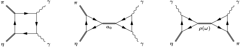
Figure 1: Diagrams contributing to the amplitude of the process $\eta\to\pi^{0}\gamma\gamma$.

The general form of the $\eta\to\pi^{0}\gamma\gamma$ decay amplitude contains two independent tensor structures Ecker et al. (1988)

$$T=T^{\mu\nu}\epsilon^{1}_{\mu}\epsilon^{2}_{\nu},\quad T^{\mu\nu}=A(x_{1},x_{2})(q_{1}^{\nu}q_{2}^{\mu}-q_{1}\cdot q_{2}g^{\mu\nu})+B(x_{1},x_{2})\left[-M_{\eta}^{2}x_{1}x_{2}g^{\mu\nu}-\frac{q_{1}\cdot q_{2}}{M_{\eta}^{2}}p^{\mu}p^{\nu}+x_{1}q_{2}^{\mu}p^{\nu}+x_{2}p^{\mu}q_{1}^{\nu}\right],$$ (7)

where $p$, $q_{1}$, $q_{2}$ are the momentum of the $\eta$ meson and photons, $\epsilon^{1}_{\mu}$ and $\epsilon^{2}_{\nu}$ are the polarization vectors of the photons, and $x_{i}=p\cdot q_{i}/M_{\eta}^{2}$.

The $\eta\to\pi^{0}\gamma\gamma$ decay width has the form

$$\Gamma = \frac{M_{\eta}^{5}}{256\pi^{2}}\int\limits_{0}^{(1-y)/2}dx_{1}\int\limits_{x_{2}^{\mathrm{min}}}^{x_{2}^{\mathrm{max}}}dx_{2}\left\{\left|A(x_{1},x_{2})+\frac{1}{2}B(x_{1},x_{2})\right|^{2}\left[2(x_{1}+x_{2})+y-1\right]^{2}\right.$$

$$+ \left.\frac{1}{4}\left|B(x_{1},x_{2})\right|^{2}\left[4x_{1}x_{2}-\left[2(x_{1}+x_{2})+y-1\right]\right]^{2}\right\},$$

$$x_{2}^{\mathrm{min}}={(1-2x_{1}-y)/2},\quad x_{2}^{\mathrm{max}}={(1-2x_{1}-y)/2(1-2x_{1})},\quad y=M_{\pi}^{2}/M_{\eta}^{2}.$$

In the NJL model the amplitude for the $\eta\to\pi^{0}\gamma\gamma$ decay process is described by three types of diagrams (see Fig. 1): the quark box and exchange of scalar($a_{0}$) and vector ($\rho,\omega$) resonances. Let us consider theses contributions in detail.

The scalar meson exchange has the simplest form. It gives a contribution only to $A(x_{1},x_{2})$. This contribution consists of three parts and can be written in the form (see appendices B and C for the definition of polarization loops and vertex functions):

$$A(x_{1},x_{2}) = \frac{g_{a_{0}\eta\pi}(2q_{1}\cdot q_{2})g_{a_{0}\gamma\gamma}(2q_{1}\cdot q_{2})}{G_{a_{0}}^{-1}-\Pi_{SS}^{uu}(2q_{1}\cdot q_{2})},\quad q_{1}\cdot q_{2}=M_{\eta}^{2}\left(x_{1}+x_{2}-\frac{1}{2}\right)+\frac{M_{\pi}^{2}}{2}$$

$$g_{a_{0}\gamma\gamma}(p^{2}) = \frac{1}{2\pi^{2}}\int\limits_{0}^{1}dx_{1}\int\limits_{0}^{1-x_{1}}dx_{2}\frac{m_{u}(1-4x_{1}x_{2})}{(p^{2}x_{1}x_{2}-m_{u}^{2}-\Lambda^{2})^{2}(p^{2}x_{1}x_{2}-m_{u}^{2})}$$ (9)

$$g_{a_{0}\eta\pi}(p^{2}) = -i2N_{c}N_{f}\int\frac{d^{4}_{\Lambda}k}{(2\pi)^{4}}\mathrm{Tr}_{D}\left\{V_{a_{0}}S_{u}(k+q_{1})V_{\pi}S_{u}(k)V_{\eta}S_{u}(k-q_{2})\right\}.$$

here $\mathrm{Tr}_{D}$ is the trace over Dirac indices, index $\Lambda$ in the measure of integration means PV regularization of the integral and $S_{j}(p)=(\hat{p}-m_{j})^{-1}$.

The amplitude with the vector meson ($\rho,\omega$) exchanges consists of two quark triangles of anomalous type (see appendix D) and the vector meson propagator. It gives the following contributions

$$B(x_{1},x_{2}) = \sum\limits_{j=\rho,\omega}\,\sum\limits_{i=1,2}\frac{g_{\eta j\gamma}(M_{\eta}^{2},M_{\eta}^{2}(1-2x_{i}),0)g_{\pi j\gamma}(M_{\pi}^{2},M_{\eta}^{2}(1-2x_{i}),0)}{G_{2}^{-1}-\Pi_{VV}^{uu}(M_{\eta}^{2}(1-2x_{i}))},$$ (10)

$$A(x_{1},x_{2}) = \sum\limits_{j=\rho,\omega}\,\sum\limits_{i=1,2}\frac{g_{\eta j\gamma}(M_{\eta}^{2},M_{\eta}^{2}(1-2x_{i}),0)g_{\pi j\gamma}(M_{\pi}^{2},M_{\eta}^{2}(1-2x_{i}),0)M_{\eta}^{2}(1-x_{i})}{G_{2}^{-1}-\Pi_{VV}^{uu}(M_{\eta}^{2}(1-2x_{i}))}.$$

The box diagram is of a more complicated structure. It consists of three types of boxes (plus three crossed) and contains the diagrams with pseudoscalar and axial-vector components of the $\pi$ and $\eta$ mesons

$$T_{\mu\nu}=-ie^{2}\int\frac{d^{4}_{\Lambda}k}{(2\pi)^{4}}\mathrm{Tr}_{D}\biggl{(}\biggr{.} V_{\pi}S(k)V_{\eta}S(k+p-q_{1}-q_{2})\gamma_{\nu}S(k+p-q_{1})\gamma_{\mu}S(k+p)+$$

$$+V_{\pi}S(k)V_{\eta}S(k+q_{2})\gamma_{\nu}S(k+p-q_{1})\gamma_{\mu}S(k+p)$$

$$+V_{\pi}S(k)\gamma_{\nu}S(k+q_{2})\gamma_{\mu}S(k+q_{1}+q_{2})V_{\eta}S(k+p)+\left\{q_{1}\leftrightarrow q_{2},\mu\leftrightarrow\nu\right\}\biggl{.}\biggr{)}$$

We calculate these diagrams numerically. In order to check the integration procedure, we calculate all coefficients of different tensor structures and verify if they have gauge invariant form (7).

The obtained results for the decay width are given in the Table 1 for two sets of model parameters. The main contribution comes from the box diagram. The contribution from vector mesons has a constructive interference while the scalar $a_{0}$ contribution has a destructive one. The results are in satisfactory agreement with Crystal Ball data $0.45\pm 0.12$ Prakhov et al. (2005) and the present value $0.57\pm 0.21$ given in PDGYao et al. (2006).

Table 1: $\eta\to\pi^{0}\gamma\gamma$ decay width.

Contribution	model 1	model 2
vector mesons	0.17	0.20
scalar meson	0.03	0.12
vector+scalar mesons	0.10	0.12
box	0.28	0.35
box+vector	0.78	0.95
total	0.53	0.45

It is also very instructive to consider the invariant mass distribution. In Figures 2 and 3 the invariant mass distribution of the two-photons is shown for the scalar meson contribution, vector mesons contribution, scalar + vector mesons and total. In Figure 4, the results of our calculations of the invariant mass distribution are compared with the calculation in the chiral unitary approach Oset et al. (2003).

Figure 2: Invariant mass distribution of the two-photons of the scalar meson contribution(dots), vector meson contributions(short dash), scalar + vector mesons(dash-dot), quark box(long dash) and total(continuous line) for the set I.

Figure 3: Invariant mass distribution of the two-photons of the scalar meson contribution(dots), vector meson contributions(short dash), scalar + vector mesons(dash-dot) , quark box(long dash) and total(continuous line) for the set II.

Figure 4: Invariant mass distribution of the two-photons of the total contributions for the set I(dashes), set II(dots) together with the results of the chiral unitary approach Oset et al. (2003).

IV Conclusions

Earlier calculations of the process $\eta\to\pi^{0}\gamma\gamma$ in the NJL model do not include the momentum dependence of quark loops and pseudoscalar–axial-vector transitions and are in satisfactory agreement with the GAMS experiment.

Recently, the new experimental data on this decay have been obtained and the value of the decay width is almost two times smaller. A number of theoretical estimates is also obtained, and it seems that the momentum dependence of amplitudes is important for a correct description of this process ( “all-order” estimate in ChPT).

In the present work, the contributions from quark box, scalar and vector pole diagrams are considered with the full momentum dependence. The pseudoscalar–axial-vector transitions are also taken into account.

The obtained result is consistent with recent experiments, theoretical estimates of ChPT Ametller et al. (1992); Bellucci and Bruno (1995) and the chiral unitary approachOset et al. (2003).

In future, we plan to consider the polarizability of pions and also decays of vector mesons $\rho(\omega)\to\eta(\pi)\pi\gamma$.

Appendixes

IV.1 Lagrangian

Lagrangian (1) can be rewritten in the form (see Klimt et al. (1990); Klevansky (1992))

$$\mathcal{L}={\bar{q}}(i{\hat{\partial}}-m^{0})q+{\frac{1}{2}}\sum_{i=1}^{9}[G_{i}^{(-)}({\bar{q}}{\lambda^{\prime}}_{i}q)^{2}+G_{i}^{(+)}({\bar{q}}i{\gamma}_{5}{\lambda^{\prime}}_{i}q)^{2}]+$$

$$\qquad+G^{(-)}_{us}({\bar{q}}{\lambda}_{u}q)({\bar{q}}{\lambda}_{s}q)+G^{(+)}_{us}({\bar{q}}i{\gamma}_{5}{\lambda}_{u}q)({\bar{q}}i{\gamma}_{5}{\lambda}_{s}q)+\frac{G_{V}}{2}\sum_{i=0}^{8}[({\bar{q}}{\gamma}_{\mu}{\lambda}_{i}q)^{2}+({\bar{q}}{\gamma}_{5}{\gamma}_{\mu}{\lambda}_{i}q)^{2}],$$ (12)

where

$${\lambda^{\prime}}_{i}={\lambda}_{i}~{}~{}~{}(i=1,...,7),~{}~{}~{}\lambda^{\prime}_{8}=\lambda_{u}=({\sqrt{2}}\lambda_{0}+\lambda_{8})/{\sqrt{3}},$$

$$\lambda^{\prime}_{9}=\lambda_{s}=(-\lambda_{0}+{\sqrt{2}}\lambda_{8})/{\sqrt{3}},$$ (13)

$$G_{1}^{(\pm)}=G_{2}^{(\pm)}=G_{3}^{(\pm)}=G\pm 4Km_{s}I_{1}(m_{s}),$$

$$G_{4}^{(\pm)}=G_{5}^{(\pm)}=G_{6}^{(\pm)}=G_{7}^{(\pm)}=G\pm 4Km_{u}I_{1}(m_{u}),$$

$$G_{u}^{(\pm)}=G\mp 4Km_{s}I_{1}(m_{s}),~{}~{}~{}G_{s}^{(\pm)}=G,~{}~{}~{}G_{us}^{(\pm)}=\pm 4{\sqrt{2}}Km_{u}I_{1}(m_{u}).$$

IV.2 Polarization loops

Polarization loops in different channels after the PV regularization

$$e^{-izm_{i}m_{j}}\to R_{ij}(z)=e^{-izm_{i}m_{j}}\left[1-(1+iz\Lambda^{2})e^{-iz\Lambda^{2}}\right]$$ (14)

take the form (see Bernard et al. (1996) for the expressions for the polarization loops with equal indices)

$$\Pi_{PP}^{ij}(p^{2}) = \frac{N_{c}}{4\pi^{2}}\int_{-1}^{1}dy\int_{0}^{\infty}\frac{dz}{z}R_{ij}(z)e^{izA}\left[-\frac{i}{z}+\frac{1}{2}p^{2}(1-y^{2})-\frac{1}{2}\left[(m_{i}-m_{j})^{2}-y(m_{i}^{2}-m_{j}^{2})\right]\right],$$

$$\Pi_{SS}^{ij}(p^{2}) = \Pi_{PP}^{ij}(p^{2})-2m_{i}m_{j}\frac{N_{c}}{4\pi^{2}}\int_{-1}^{1}dy\int_{0}^{\infty}\frac{dz}{z}R_{ij}(z)e^{izA},$$

$$\Pi_{VV}^{ij,{\mu\nu}}(p^{2}) = \left(g^{\mu\nu}-\frac{p^{\mu}p^{\nu}}{p^{2}}\right)\Pi_{VV}^{ij}(p^{2})+\frac{p^{\mu}p^{\nu}}{p^{2}}\Pi_{VV}^{ij,L}(p^{2}),$$

$$\Pi_{VV}^{ij,L}(p^{2}) = \frac{N_{c}}{8\pi^{2}}\int_{-1}^{1}dy\int_{0}^{\infty}\frac{dz}{z}R_{ij}(z)e^{izA}\left[(m_{i}-m_{j})^{2}-y(m_{i}^{2}-m_{j}^{2})\right],$$

$$\Pi_{VV}^{ij}(p^{2}) = \Pi_{VV}^{ij,L}(p^{2})-p^{2}\frac{N_{c}}{8\pi^{2}}\int_{-1}^{1}dy(1-y^{2})\int_{0}^{\infty}\frac{dz}{z}R_{ij}(z)e^{izA},$$

$$\Pi_{AA}^{ij,{\mu\nu}}(p^{2}) = \left(g^{\mu\nu}-\frac{p^{\mu}p^{\nu}}{p^{2}}\right)\Pi_{AA}^{ij,T}(p^{2})+\frac{p^{\mu}p^{\nu}}{p^{2}}\Pi_{AA}^{ij}(p^{2}),$$

$$\Pi_{AA}^{ij,T}(p^{2}) = \Pi_{VV}^{ij}(p^{2})+2m_{i}m_{j}\frac{N_{c}}{4\pi^{2}}\int_{-1}^{1}dy\int_{0}^{\infty}\frac{dz}{z}R_{ij}(z)e^{izA},$$ (15)

$$\Pi_{AA}^{ij}(p^{2}) = \Pi_{VV}^{ij,L}(p^{2})+2m_{i}m_{j}\frac{N_{c}}{4\pi^{2}}\int_{-1}^{1}dy\int_{0}^{\infty}\frac{dz}{z}R_{ij}(z)e^{izA},$$

$$\Pi_{PA}^{ij,\mu}(p^{2}) = \frac{p^{\mu}}{\sqrt{p^{2}}}\Pi_{PA}^{ij}(p^{2})=p^{\mu}i(m_{i}+m_{j})\frac{N_{c}}{8\pi^{2}}\int_{-1}^{1}dy\int_{0}^{\infty}\frac{dz}{z}R_{ij}(z)e^{izA},$$

$$\Pi_{AP}^{ij,\mu}(p^{2}) = \frac{p^{\mu}}{\sqrt{p^{2}}}\Pi_{AP}^{ij}(p^{2})=-p^{\mu}i(m_{i}+m_{j})\frac{N_{c}}{8\pi^{2}}\int_{-1}^{1}dy\int_{0}^{\infty}\frac{dz}{z}R_{ij}(z)e^{izA},$$

$$A=\frac{p^{2}}{4}(1-y^{2})-\frac{1}{2}\left[(m_{i}-m_{j})^{2}-y(m_{i}^{2}-m_{j}^{2})\right].$$

IV.3 Vertex functions

The most simple form have the vertex functions for the vector $\rho$ and the isovector scalar meson $a_{0}$, namely :

$$V_{a_{0}}=g_{a_{0}}\mathbf{I}a_{0},\quad V_{\rho}=g_{\rho}\gamma_{\mu}\rho^{\mu}.$$ (16)

The matrices $\mathbf{G}$ and $\mathbf{\Pi}$ for $a_{0}$ and $\rho$ mesons have the form

$$\mathbf{G}_{a_{0}} = G_{1}^{(-)},\,\mathbf{\Pi}_{a_{0}}(p^{2})=\Pi_{SS}^{uu}(p^{2}),$$ (17)

$$\mathbf{G}_{\rho} = G_{2}\quad,\mathbf{\Pi}_{\rho}(p^{2})=\Pi_{VV}^{uu}(p^{2})$$

For the pion and kaon, additional axial-vector components appear in the vertex function due to pseudoscalar–axial-vector mixing

$$V_{\pi}=g_{\pi}i\gamma_{5}(1+\Delta_{\pi}\hat{p})\pi,\,\quad V_{K}=g_{K}i\gamma_{5}(1+\Delta_{K}\hat{p})K$$ (18)

Here $\mathbf{G}$ and $\mathbf{\Pi}$ are

$$\mathbf{G}_{\pi}=\begin{pmatrix}G_{1}^{(+)}&0\\ 0&G_{2}\end{pmatrix},\mathbf{\Pi}_{\pi}(p^{2})=\begin{pmatrix}\Pi^{uu}_{PP}(p^{2})&\Pi^{uu}_{PA}(p^{2})\\ \Pi^{uu}_{AP}(p^{2})&\Pi^{uu}_{AA}(p^{2})\end{pmatrix},$$ (19)

$$\mathbf{G}_{K}=\begin{pmatrix}G_{4}^{(+)}&0\\ 0&G_{2}\end{pmatrix},\mathbf{\Pi}_{K}(p^{2})=\begin{pmatrix}\Pi^{us}_{PP}(p^{2})&\Pi^{us}_{PA}(p^{2})\\ \Pi^{us}_{AP}(p^{2})&\Pi^{us}_{AA}(p^{2})\end{pmatrix}.$$

Therefore, the vertex function of the $\eta$ meson have four components: strange and non-strange pseudoscalar and axial-vector

$$V_{\eta} = g_{\eta_{u}}i\gamma_{5}(1+\Delta_{\eta_{u}}\hat{p})\eta_{u}+g_{\eta_{s}}i\gamma_{5}(1+\Delta_{\eta_{s}}\hat{p})\eta_{s}=$$

$$= g_{\eta}i\gamma_{5}(\cos\Theta_{\eta}\eta_{u}-\sin\Theta_{\eta}\eta_{s}+\Delta_{\eta}\hat{p}(\cos\widetilde{\Theta}_{\eta}\eta_{u}-\sin\widetilde{\Theta}_{\eta}\eta_{s})),$$

where $\Theta_{\eta}$ and $\widetilde{\Theta}_{\eta}$ are the mixing angles for pseudoscalar and axial-vector components. The matrices $\mathbf{G}$ and $\mathbf{\Pi}(p^{2})$ are four-by-four matrices

$$\mathbf{G}=\begin{pmatrix}\mathbf{G}^{(+)}&0\\ 0&\mathbf{G_{2}}\end{pmatrix},\mathbf{G}^{(+)}=\begin{pmatrix}G_{u}^{(+)}&G_{us}^{(+)}\\ G_{us}^{(+)}&G_{s}^{(+)}\end{pmatrix},\mathbf{G_{2}}=\mathrm{diag}\{G_{2},G_{2}\}$$ (21)

$$\mathbf{\Pi}(p^{2})=\begin{pmatrix}\mathbf{\Pi}_{PP}(p^{2})&\mathbf{\Pi}_{PA}(p^{2})\\ \mathbf{\Pi}_{AP}(p^{2})&\mathbf{\Pi}_{AA}(p^{2})\end{pmatrix},\mathbf{\Pi}_{ij}(p^{2})=\mathrm{diag}\{\Pi^{uu}_{ij(p^{2})},\Pi^{ss}_{ij}(p^{2})\},i,j=P,A$$

IV.4 Amplitudes $\eta\to\gamma\gamma$, $\rho\to\eta(\pi)\gamma$

The amplitude for the two-photon decay width of the pseudoscalar meson has the form

$$A(P\to\gamma\gamma)\ =\ e^{2}\;g_{P\gamma\gamma}(M_{P}^{2},q_{1}^{2},q_{2}^{2})\ \epsilon_{\mu\nu\alpha\beta}\ \epsilon_{1}^{\mu}\epsilon_{2}^{\nu}\;q_{1}^{\alpha}q_{2}^{\beta}\ ,$$ (22)

where $q_{1}$, $q_{2}$ are the momentum of photons and $\epsilon^{1}_{\mu}$, $\epsilon^{2}_{\nu}$ are the polarization vectors of the photons,

$$g_{\pi\gamma\gamma}(M_{\pi}^{2},q_{1}^{2},q_{2}^{2}) = I_{u}(M_{\pi}^{2},q_{1}^{2},q_{2}^{2})g_{\pi},$$ (23)

$$g_{\eta\gamma\gamma}(M_{\eta}^{2},q_{1}^{2},q_{2}^{2}) = \frac{5}{3}I_{u}(M_{\eta}^{2},q_{1}^{2},q_{2}^{2})g_{\eta_{u}}-\frac{\sqrt{2}}{3}I_{s}(M_{\eta}^{2},q_{1}^{2},q_{2}^{2})g_{\eta_{s}}.$$

The loop integrals $I_{j}(M_{P}^{2})$ are given by

$$I_{j}(M_{P}^{2},q_{1}^{2},q_{2}^{2}) = \frac{1}{2\pi^{2}}\int\limits_{0}^{1}dx_{1}\int\limits_{0}^{1-x_{1}}dx_{2}\frac{m_{j}}{m_{j}^{2}-x_{1}(1-x_{1}-x_{2})q_{1}^{2}-x_{2}(1-x_{1}-x_{2})q_{2}^{2}-x_{1}x_{2}M_{P}^{2}}.$$ (24)

The amplitudes for the processes $\rho(\omega)\to\eta(\pi)\gamma$ have the form

$$A(PV\gamma)\ =\ g_{\rho}e\;g_{P\rho\gamma}(M_{P}^{2},q_{1}^{2},q_{2}^{2})\ \epsilon_{\mu\nu\alpha\beta}\ \epsilon_{1}^{\mu}\epsilon_{2}^{\nu}\;q_{1}^{\alpha}q_{2}^{\beta}\ ,$$ (25)

here $q_{1}$ and $\epsilon^{1}_{\mu}$ are the momentum and the polarization vector of $\rho(\omega)$ meson.

$$g_{\pi\rho\gamma}(M_{\pi}^{2},q_{1}^{2},q_{2}^{2}) = I_{u}(M_{\pi}^{2},q_{1}^{2},q_{2}^{2})g_{\pi},\quad g_{\eta\rho\gamma}(M_{\eta}^{2},q_{1}^{2},q_{2}^{2})=3I_{u}(M_{\eta}^{2},q_{1}^{2},q_{2}^{2})g_{\eta_{u}},$$

$$g_{\pi\omega\gamma}(M_{\pi}^{2},q_{1}^{2},q_{2}^{2}) = 3I_{u}(M_{\pi}^{2},q_{1}^{2},q_{2}^{2})g_{\pi},\quad g_{\eta\omega\gamma}(M_{\eta}^{2},q_{1}^{2},q_{2}^{2})=I_{u}(M_{\eta}^{2},q_{1}^{2},q_{2}^{2})g_{\eta_{u}}.$$ (26)

References

Achasov et al. (2001)
M. N. Achasov
et al., Nucl. Phys.
B600, 3 (2001),
eprint hep-ex/0101043.
Giugno et al. (1966)
G. D. Giugno
et al.,Phys. Rev. Lett. 16,
767 (1966).
Oppo and Oneda (1967)
G. Oppo and
S. Oneda,
Phys. Rev. 160,
1397 (1967).
Ebert and Volkov (1979)
D. Ebert and
M. K. Volkov,
Sov. J. Nucl. Phys. 30,
736 (1979).
Ivanov and Troitskaya (1982)
A. N. Ivanov and
N. I. Troitskaya,
Yad. Fiz. 36,
494 (1982).
Kreopalov and Volkov (1983)
D. V. Kreopalov
and M. K.
Volkov, Sov. J. Nucl. Phys.
37, 770 (1983).
Volkov (1986)
M. K. Volkov,
Sov. J. Part. and Nuclei
17, 186 (1986).
Binon et al. (1981)
F. Binon et al.
(Serpukhov-Brussels-Annecy(LAPP)),
Nuovo Cim. Lett. 32,
45 (1981).
Alde et al. (1984)
D. Alde et al.
(Serpukhov-Brussels-Annecy(LAPP)),
Z. Phys. C25,
225 (1984).
Prakhov et al. (2005)
S. Prakhov et al.,
Phys. Rev. C72,
025201 (2005).
Ng and Peters (1993)
J. N. Ng and
D. J. Peters,
Phys. Rev. D47,
4939 (1993).
Nemoto et al. (1996)
Y. Nemoto,
M. Oka, and
M. Takizawa,
Phys. Rev. D54,
6777 (1996), eprint hep-ph/9602253.
Ko (1993)
P. Ko, Phys.
Rev. D47, 3933
(1993).
Ng and Peters (1992)
J. N. Ng and
D. J. Peters,
Phys. Rev. D46,
5034 (1992).
Ametller et al. (1992)
L. Ametller,
J. Bijnens,
A. Bramon, and
F. Cornet,
Phys. Lett. B276,
185 (1992).
Bellucci and Bruno (1995)
S. Bellucci and
C. Bruno,
Nucl. Phys. B452,
626 (1995), eprint hep-ph/9502243.
Ko (1995)
P. Ko, Phys.
Lett. B349, 555
(1995), eprint hep-ph/9503253.
Bel’kov et al. (1996)
A. A. Bel’kov,
A. V. Lanyov,
and S. Scherer,
J. Phys. G22,
1383 (1996), eprint hep-ph/9506406.
Bijnens et al. (1996)
J. Bijnens,
A. Fayyazuddin,
and J. Prades,
Phys. Lett. B379,
209 (1996), eprint hep-ph/9512374.
Oset et al. (2003)
E. Oset,
J. R. Pelaez,
and L. Roca,
Phys. Rev. D67,
073013 (2003), eprint hep-ph/0210282.
Bernard et al. (1992)
V. Bernard,
A. A. Osipov,
and U. G.
Meissner, Phys. Lett.
B285, 119 (1992).
Bernard et al. (1996)
V. Bernard et al.,
Annals Phys. 249,
499 (1996), eprint hep-ph/9506309.
Bajc et al. (1996)
B. Bajc et al.,
Nucl. Phys. A604,
406 (1996), eprint hep-ph/9602394.
Klevansky (1992)
S. P. Klevansky,
Rev. Mod. Phys. 64,
649 (1992).
Klimt et al. (1990)
S. Klimt,
M. Lutz,
U. Vogl, and
W. Weise,
Nucl. Phys. A516,
429 (1990).
Schuren et al. (1992)
C. Schuren,
E. Ruiz Arriola,
and K. Goeke,
Nucl. Phys. A547,
612 (1992).
Yao et al. (2006)
W.-M. Yao,
et al., Journal of Physics G
33, 1 (2006),
URL http://pdg.lbl.gov.
Ecker et al. (1988)
G. Ecker,
A. Pich, and
E. de Rafael,
Nucl. Phys. B303,
665 (1988).