Small-$x$ Dipole Evolution Beyond the Large-$N_{c}$ Limit

Abstract:

We present a method to include colour-suppressed effects in the Mueller dipole picture. The model consistently includes saturation effects both in the evolution of dipoles and in the interactions of dipoles with a target in a frame-independent way.

When implemented in a Monte Carlo simulation together with our previous model of energy–momentum conservation and a simple dipole description of initial state protons and virtual photons, the model is able to reproduce to a satisfactory degree both the $\gamma^{*}p$ cross sections as measured at HERA as well as the total $pp$ cross section all the way from ISR energies to the Tevatron and beyond.

1 Introduction

Parton evolution at small $x$ is a difficult problem. It is interesting because of the strong nonlinear effects and the interplay between perturbative and non-perturbative physics, and it is an important problem, as it is necessary to have a good understanding of the dominant effects from the strong interaction in the analyses of results from LHC and the interpretation of possible signals for new physics.

Although it cannot be possible to include all quantum interference effects in a classical branching process, such a stochastic evolution has been extremely successful to describe parton cascades in $e^{+}e^{-}$-annihilation. This is also the case in the DGLAP regime of DIS (high $Q^{2}$ and large $x$). In these cases the virtuality or transverse momentum acts as a well-defined evolution parameter, and the perturbative cascade can be well separated from the non-perturbative effects in the hadronization or the input distributions in the DGLAP evolution. We note, however, that important for the good agreement with LEP data is both a description of the hardest gluons by fixed order matrix elements, and implementation of energy–momentum conservation in the event simulation procedure.

DIS at small $x$ is more difficult. To LL or NLL accuracy the cross section is determined by the BFKL equation, which describes an evolution in $x$ instead of the $k_{\perp}$-ordering in the DGLAP evolution. A big problem is here that the NLL corrections are so large, that it in practice only can give a qualitative description of experimental data.

Part of the NLL corrections originate from the running coupling $\alpha_{s}$. Including a running coupling in the evolution implies that the parton chain spreads into the non-perturbative region, and a soft cutoff is needed for small $k_{\perp}$. This problem is avoided in studies of collisions between highly virtual photons or massive onium states. Another possibility is to study events with two high $p_{\perp}$ jets separated by a large rapidity interval. Also here it is demonstrated that the energy–momentum conservation constraint has a very large effect on the theoretical calculations [1]. In $ep$ and $pp$ scattering the influence of non-perturbative effects cannot be avoided, however, and has to be included in the analysis.

A most essential feature of the $e^{+}e^{-}$-cascades is the so-called ”soft colour interference” or angular ordering [2, 3, 4, 5]. A colour charge in one parton has always a corresponding anti-charge in an accompanying parton, and it is important to account for the interference in the radiation from these emitters. An efficient way to treat this effect is offered by the dipole cascade model described in refs. [6, 7], in which the QCD state is described as a chain of colour dipoles formed by a charge–anti-charge pair, rather than a chain of gluons. In the large $N_{c}$ limit the dipoles radiate independently, and analyses of experimental data from LEP [8, 9, 10, 11] indicate that the interference between different dipoles is very weak. (In contrast to the other three LEP experiments, DELPHI [11] does indeed favour some weak effects from interaction.)

In DIS a formulation with coherent colour dipoles was presented by Golec-Biernat–Wüsthoff[12, 13], and a space-like dipole cascade model was formulated by Mueller [14, 15, 16]. While the time-like dipole cascade model in ref. [7] is formulated in momentum space, the dipoles in these models are specified in transverse coordinate (or impact parameter) space. As the transverse coordinate is little affected in a high energy interaction, this makes it possible to account for multiple parton sub-collisions in a natural way.

Mueller’s dipole cascade model is valid in the large $N_{c}$ limit, and is demonstrated to satisfy the BFKL equation to LL accuracy. In this picture one starts with a $q\bar{q}$ colour singlet state (a quarkonium or simply onium state), and when the system is boosted to higher energy more and more soft gluons are emitted, forming a chain of colour dipoles. As mentioned this approach leads to the BFKL equation, but it also goes beyond the BFKL formalism. When two cascades collide it is possible to take into account multiple scattering to all orders, and it is thus possible to obtain a unitarised expression for the $S$-matrix. The probabilistic nature of the cascades implies that the evolution can be simulated in a Monte Carlo program, and the effects of unitarisation be studied numerically [17, 18] (see also [19]).

The dipole model contains a vertex in which a dipole splits into two new dipoles, originating when a soft gluon is emitted from the original colour dipole. The evolution can then be formulated as a typical birth–death process, where a dipole can decay into two new dipoles with a specified differential probability, proportional to $dY$, with $Y=\log 1/x$ which here acts as a time variable for the evolution process.

There are some problems with the dipole evolution as formulated in [14, 15, 16]. One problem comes from the fact that the cascade cannot correspond to real gluon emissions. The splitting vertex diverges as the size of one of the new dipoles goes to zero. The many small dipoles interact, however, very weakly with a target, a phenomenon referred to as colour transparency. Thus, even if the number of small dipoles diverges, the total cross section remains finite. Although we thus get a finite cross section, the divergence causes problems: i) Dipoles which do not interact should be regarded as virtual. Therefore the dipole model in this formulation can be used to study fully inclusive quantities like the total cross section, but not the properties of exclusive final states. ii) In numerical calculations the divergence has to be regulated by a cutoff for small dipoles. Although the cutoff does not show up in the cross section, it makes it extremely time consuming to run a simulation program with a cutoff, which is small enough to simulate the physics with good accuracy.

As mentioned above, the constraint from energy–momentum conservation is very important in order to achieve agreement between theory and experiment in $e^{+}e^{-}$-annihilation, and in [1] it is demonstrated that it also has a large effect in space-like cascades. This constraint goes beyond the LL approximation, and is not included in the formalism in [14, 15]. This is related to the problem with small dipoles discussed above. A very small dipole corresponds to well localized partons, which thus must have large transverse momenta, which in turn implies also non-negligible longitudinal momentum and energy. Only real final state partons have to obey conservation of energy and momentum, and to fully solve this problem one must also solve the problem with specifying the final states.

Another problem is due to the fact that in this formalism dipoles in the same onium do not interact. Saturation effects are included in the collisions between two cascades, but not in the evolution of each cascade separately. This problem is related to the large $N_{c}$ approximation in the evolution. Multiple collisions are formally colour suppressed, and in the Lorentz frame where the collision is studied they lead to the formation of pomeron loops. As the evolution is only leading in colour, such loops cannot be formed during the evolution itself. If one e.g. studies the collision in a very asymmetric frame, where one of the onia carries almost all the available energy and the other is almost at rest, then the possibility to have multiple collisions is strongly reduced. Only those pomeron loops are included, which are cut in the specific Lorentz frame used for the calculations, which obviously only forms a limited set of all possible pomeron loops. It implies that the dipole model is not frame independent, and the preferred Lorentz frame is the one where the two colliding systems have approximately the same density of dipoles . This feature clearly limits the rapidity range of validity. It is apparent that a frame independent formulation must include colour suppressed interactions between the dipoles during the evolution of the cascades, but so far it has not been possible to formulate a model, which includes saturation effects and is explicitely frame independent.

There is also another related problem with the finite number of colour charges. The dipole degrees of freedom are natural only in the $N_{c}\rightarrow\infty$ limit. Consider for example a system of $r\bar{r}r\bar{r}$ charges. Using the dipole basis this system the colours can be combined in two different ways. Obviously, to go beyond large $N_{c}$ one would need to take into account quadrupoles, as in the example above, and even higher multipoles. This makes the colour structure of the gluon cascade really non-trivial, and one loses the picture of a system of dipoles evolving through dipole splittings in a stochastic process. As the dipole approximation is so successful in $e^{+}e^{-}$-annihilation, it may still be possible to find a working approximation using only dipoles. In the example above it may be possible to describe the quadrupole field as two dipoles formed by the closest charge–anti-charge pairs. Such an approximate scheme can be realized by introducing a $2\rightarrow 2$ transition vertex in the dipole evolution.

In this paper we want to discuss ways to improve the dipole description of high energy interaction in DIS and hadronic collisions. Some effects of energy–momentum conservation were presented in ref. [20]. This constraint gives a dynamic cutoff for small dipoles, which strongly reduces some of the problems discussed above. The dipole multiplicity is reduced, which makes the Monte Carlo simulation much more efficient. The reduced dipole multiplicity also reduces the effect of saturation, which becomes rather small for DIS within the HERA kinematical region. Here we will further extend the model presented in [20], including colour suppressed effects related to pomeron loops by introducing a $2\rightarrow 2$ transition vertex in the dipole evolution. Although not explicitely frame independent, the dependence on the Lorentz frame used is here much reduced.

The coupling of a virtual photon to a $q\bar{q}$ dipole is well known, but the proton is a much more complicated system. It was early suggested that semi-hard parton sub-collisions and minijets are important ingredients in high energy $pp$ collisions, and responsible for the rising cross section [21, 22, 23, 24]. This picture is supported by the successful description of Tevatron data [25] using the Pythia MC, which is based on perturbative parton–parton collisions [26]. These results encourages us to describe high energy $\gamma^{*}p$ and $pp$ collisions in terms of perturbative dipole–dipole collisions, and we will in this paper also present a simple model for the initial dipole system in a proton. The ideas are implemented in a computer simulation program, and the results are compared with DIS data from HERA and with data from hadron–hadron colliders.

The paper is organized as follows. In the next section we describe the dipole picture of high energy collisions in QCD and its relation to the string picture. In section 3 we briefly summarize the alternative approach to high energy QCD, the color glass condensate, and recent results related to the formation of pomeron loops in the corresponding evolution equations. In section 4 we describe the improvements we have made in the dipole model as was briefly described in this introduction, followed in section 5 by a brief discussion of the model of the proton used to obtain quantitative results. In section 6 we present some details about our Monte Carlo program and how we implement the improvements we have made. Then, in section 7, we present the applications of these improvements and compare our results to experimental data for DIS and $pp$ scattering. Finally, in section 8, we arrive at our conclusions.

2 Dipole Picture of QCD

Higher order QCD diagrams are very difficult, and naturally it is not possible to formulate a quantum mechanical parton cascade as a classical branching process, including all interference effects. The great success for parton cascades in $e^{+}e^{-}$-annihilation is therefore quite surprising. DIS is, however, significantly more complicated than $e^{+}e^{-}$-annihilation.

2.1 Cascades in $e^{+}e^{-}$-annihilation

In $e^{+}e^{-}$ the main problem is to calculate the properties of the final states, while the total cross section is well determined by low order perturbative QCD calculations. Although the 1st order matrix element for gluon emission diverges for soft gluons, the total cross section is still finite and given by $\sigma_{tot}\approx\sigma_{0}\,(1+\alpha_{s}/\pi)$, where $\sigma_{0}$ is the cross section to 0th order in $\alpha_{s}$. The divergence for soft gluon emission is compensated by virtual corrections, which can easily be taken into account by Sudakov form factors. This implies that the cascade has a probabilistic nature; the emission of one more gluon in the ordered cascade does not change the total reaction cross section.

The process $e^{+}e^{-}\rightarrow q\bar{q}gg$ does factorize in the limit when one gluon is much softer than the other. In the large $N_{c}$ limit also the amplitude for a multi-gluon final state factorizes in the strongly ordered regime, where one gluon is much softer than the previous one. $N_{c}$ is, however, not a big number (even if the non-factorizing correction terms are of order $1/N_{c}^{2}$ and not $1/N_{c}$). Also the value of $\alpha_{s}$ is so large that cascades which are not strongly ordered (and therefore do not factorize), are very important in analyses of experimental data.

The result depends quite strongly on the treatment of not well ordered cascades, where the description depends equally much on physical intuition as on analytic calculations. A very essential feature is what is called soft colour interference, which was mentioned in the introduction. A parton with e.g. a red colour has always a partner carrying anti-red colour charge. The interference between these two charges implies a suppression for emission of gluons with wavelengths larger than the separation between the emitters. Thus the colour charge and its anti-charge partner do not radiate independently, but must be treated as one unit.

In a fixed Lorentz frame this interference effect can be approximated by an angular ordering [2, 3, 4, 5]. This means that emissions from the red and anti-red partons is restricted to angular cones with opening angles equal to the angle between the emitters. This angular constraint is not Lorentz invariant but frame dependent. It also overestimates the emission in some directions and underestimates it in other, but in such a way that it averages out to the correct value.

A different approach to this effect is given by the dipole cascade model described in [6, 7]. In this model the QCD state is described as a chain of colour dipoles (with given momentum, energy, and orientation) rather than a chain of gluons (with momentum, energy, and polarization). This is similar to the relation between a lattice and its dual lattice. It is interesting to note that at the end of the cascade this dipole chain gives a smooth transition to the string in the Lund fragmentation model [27]. In the large $N_{c}$ limit the dipoles radiate independently apart from recoils (which may be important when the emissions are not strongly ordered). The radiation from the dipole formed by the red and anti-red charges discussed above is studied in the rest frame of the two partons forming that dipole. Boosting to e.g. the overall rest frame this reproduces the angular ordering, but without the (unrealistic) sharp angular cutoff. A comparison between the dipole approximation and the exact 2nd order matrix element is given in [28].

The angular ordering constraint is implemented in the event generators Herwig [29] and Pythia [30], and the dipole cascade in the Ariadne event generator [31]. They all give very good descriptions of experimental data from LEP and other $e^{+}e^{-}$ colliders, with the dipole model giving just a slightly better overall $\chi^{2}$. (The overall structure of the final state depends strongly on the first hard emissions, and in all approaches the best agreement is obtained if these are described by fixed order matrix elements.)

2.2 Cascades in DIS

DIS is a more complicated process than $e^{+}e^{-}$-annihilation. First, there are in DIS two different energy scales, $W^{2}$ and $Q^{2}$. Secondly, in DIS both the cross section and the final state properties are highly nontrivial problems. Only in the pure DGLAP region, with high $Q^{2}$ and large $x$, has the probabilistic description in terms of $k_{\perp}$-ordered cascades been really successful, in this case both for cross sections and final state properties. In the DGLAP region the real emissions are compensated by virtual corrections in a way similar to the time-like cascades in $e^{+}e^{-}$-annihilation. Thus the virtual corrections can also here be treated by Sudakov form factors, and the cascade contains only the real emissions appearing in the final state. Thus the DGLAP evolution describes the probability for a given parton state with a fixed resolution determined by $Q^{2}$. The total cross section is determined by the reaction probability between the virtual photon and the quarks in the cascade. The final state is obtained by adding final state radiation to the partons in the initial cascade (within angular ordered regions).

For lower $x$ and $Q^{2}$ separate approaches have been used to describe the total cross section and the final state properties. To LL or NLL accuracy the cross section is determined by the BFKL equation. The BFKL evolution can be formulated in different ways. In its implementation in the Mueller dipole cascade it is not suited to describe the final state, as the evolution contains a very large number of virtual dipoles, which do not appear as final state particles. As mentioned, the BFKL equation has also the problem that the NLL corrections are so very large.

The presently best description of the final state properties at HERA is given by the soft radiation model (frequently called the Color Dipole Model, CDM, and implemented in the Ariadne event generator). In this model the gluon radiation from the separating colour charges in the kicked out quark and the proton remnant is described in a way analogous to emission in $e^{+}e^{-}$-annihilation. The CDM model does not predict the cross section, but only the properties of the final state. It has also the drawback that it is not solidly founded in perturbative QCD.

The CCFM model [32, 33] represents an interpolation between the DGLAP and BFKL evolutions. In the DGLAP region the cascade contains, besides the real emissions in the DGLAP equation, also softer emissions which are treated as final state radiation in the DGLAP approach. This makes the regions where final state radiation should be added more complicated, and a description of final state properties more difficult. The CCFM model is reformulated and generalized in the Linked Dipole Chain (LDC) model [34], which is based on a different separation between initial and final state radiation. Both these models are implemented in MC event generators, Cascade[35, 36] and LDCMC[37, 38] respectively. The models have the ambition to describe both the cross section and the final state properties. They both work well with respect to the cross sections, but none is as successful as the abovementioned CDM model, when it comes to the properties of the final states.

2.3 Mueller’s Dipole Formulation

The Mueller dipole model [14, 15, 16] is formulated in transverse coordinate space. Such a formulation has the advantage that the transverse coordinates of the partons are not changed during the evolution. This makes it easier to take into account saturation effects due to multiple scatterings. On the other hand, it is easier to take into account energy–momentum conservation in a model formulated in transverse momentum space.

In Mueller’s model we start with a $q\bar{q}$ pair, heavy enough for perturbative calculations to be applicable, and calculate the probability to emit a soft gluon from this pair. Here the quark and the antiquark are assumed to follow light-cone trajectories and the emission of the gluon is calculated in the eikonal approximation in which the emitters do not suffer any recoil. Adding the contributions to the emission from the quark and the antiquark, including the interference, one obtains the result (for notations, see figure 1)

$$\frac{d\mathcal{P}}{dY}=\frac{\bar{\alpha}}{2\pi}d^{2}\boldsymbol{z}\frac{(\boldsymbol{x}-\boldsymbol{y})^{2}}{(\boldsymbol{x}-\boldsymbol{z})^{2}(\boldsymbol{z}-\boldsymbol{y})^{2}}\equiv\frac{\bar{\alpha}}{2\pi}d^{2}\boldsymbol{z}\mathcal{M}(\boldsymbol{x},\boldsymbol{y},\boldsymbol{z}).$$ (1)

Here $\boldsymbol{x}$, $\boldsymbol{y}$, and $\boldsymbol{z}$ are two-dimensional vectors in transverse coordinate space and $Y$ denotes the rapidity, which acts as the time variable in the evolution process.

Figure 1: The evolution of the dipole cascade. At each step, a dipole can split into two new dipoles with decay probability given by (1).

This formula can be interpreted as the emission probability from a dipole located at $(\boldsymbol{x},\boldsymbol{y})$. In the large $N_{c}$ limit the gluon can be seen as a quark–antiquark pair and the formula above can then be interpreted as the decay of the original dipole $(\boldsymbol{x},\boldsymbol{y})$ into two new dipoles, $(\boldsymbol{x},\boldsymbol{z})$ and $(\boldsymbol{z},\boldsymbol{y})$. In the same limit further emissions factorize, so that at each step one has a chain of dipoles where each dipole can decay into two new dipoles with the decay probability given by (1). In this way one obtains a cascade of dipoles which evolve through dipole splittings, and the number of dipoles grows exponentially with $Y$.

We note that the expression above has non-integrable singularities at $\boldsymbol{z}=\boldsymbol{x}$ and $\boldsymbol{z}=\boldsymbol{y}$. In numerical calculations it is therefore necessary to introduce a cutoff, $\rho$, such that $(\boldsymbol{x}-\boldsymbol{z})^{2},(\boldsymbol{z}-\boldsymbol{y})^{2}\geq\rho^{2}$. To obtain a meaningful probabilistic interpretation of (1) (note that $d\mathcal{P}/dY$ can become very large for small $\rho$) we also need to take into account virtual corrections to the real emissions. The effect of these corrections is described by a Sudakov form factor, $S=$exp$(-\int dYd^{2}\boldsymbol{z}\cdot d\mathcal{P}/dY)$, which should multiply the splitting probability in (1).

2.4 Scattering of Dipoles

In Mueller’s model each dipole interacts independently with some target via two-gluon exchange. In case of onium–onium scattering each onium evolves into a cascade of dipoles. We let $f_{ij}$ denote the imaginary part of the elastic scattering amplitude for a dipole $i$, with coordinates $(\boldsymbol{x}_{i},\boldsymbol{y}_{i})$, in one of the onia and a dipole $j$, with coordinates $(\boldsymbol{x}_{j},\boldsymbol{y}_{j})$, in the other onium. The basic dipole–dipole scattering amplitude from gluon exchange is given by

$$f_{ij}=\frac{\alpha_{s}^{2}}{8}\biggl{[}\log\biggl{(}\frac{(\boldsymbol{x}_{i}-\boldsymbol{y}_{j})^{2}(\boldsymbol{y}_{i}-\boldsymbol{x}_{j})^{2}}{(\boldsymbol{x}_{i}-\boldsymbol{x}_{j})^{2}(\boldsymbol{y}_{i}-\boldsymbol{y}_{j})^{2}}\biggr{)}\biggr{]}^{2}.$$ (2)

In the single pomeron approximation the onium–onium amplitude is then simply given by the sum of the basic dipole–dipole amplitudes, $\sum_{ij}f_{ij}$.

In the dipole model it is also possible to have multiple scatterings, i.e the simultaneous scatterings of several dipoles. Assuming that the individual dipole interactions are uncorrelated, summing multiple scatterings to all orders exponentiates, and the total amplitude for a single event is given by $1-$exp$(-\sum_{ij}f_{ij})$. Thus, the expansion of the exponential in a power series corresponds directly to the contributions from the multiple scattering series, where the single pomeron cross section corresponding to the first term in this series is given by $2\int\langle\sum_{ij}f_{ij}\rangle$.

Consider the scattering of an elementary dipole $(\boldsymbol{x},\boldsymbol{y})$ off some arbitrary target. We denote the scattering matrix by $\mathcal{S}(\boldsymbol{x},\boldsymbol{y})$. After one step of evolution in rapidity the dipole $(\boldsymbol{x},\boldsymbol{y})$ has a chance to split into two new dipoles, $(\boldsymbol{x},\boldsymbol{z})$ and $(\boldsymbol{z},\boldsymbol{y})$, through the splitting kernel $\mathcal{M}_{\boldsymbol{x}\boldsymbol{y}\boldsymbol{z}}\equiv\mathcal{M}(\boldsymbol{x},\boldsymbol{y},\boldsymbol{z})$. The evolution of the $S$-matrix is then given by

$$\partial_{Y}\mathcal{S}(\boldsymbol{x},\boldsymbol{y})=\frac{\bar{\alpha}}{2\pi}\int d^{2}\boldsymbol{z}\mathcal{M}_{\boldsymbol{x}\boldsymbol{y}\boldsymbol{z}}\{-\mathcal{S}(\boldsymbol{x},\boldsymbol{y})+\mathcal{S}^{(2)}(\boldsymbol{x},\boldsymbol{z};\boldsymbol{z},\boldsymbol{y})\}.$$ (3)

The right hand side in this expression simply states that the dipole can remain as it is, with a reduced probability, $1-\bar{\alpha}/2\pi\int\mathcal{M}$, or that it can split into two new dipoles, $(\boldsymbol{x},\boldsymbol{z})$ and $(\boldsymbol{z},\boldsymbol{y})$, with a probability density given by (1). If we assume that $\mathcal{S}^{(2)}(\boldsymbol{x},\boldsymbol{z};\boldsymbol{z},\boldsymbol{y})=\mathcal{S}(\boldsymbol{x},\boldsymbol{z})\mathcal{S}(\boldsymbol{z},\boldsymbol{y})$ and rewrite the equation in the scattering amplitude $T\equiv 1-\mathcal{S}$, we get

$$\partial_{Y}T(\boldsymbol{x},\boldsymbol{y})=\frac{\bar{\alpha}}{2\pi}\int d^{2}\boldsymbol{z}\mathcal{M}_{\boldsymbol{x}\boldsymbol{y}\boldsymbol{z}}\{-T(\boldsymbol{x},\boldsymbol{y})+T(\boldsymbol{x},\boldsymbol{z})+T(\boldsymbol{z},\boldsymbol{y})-T(\boldsymbol{x},\boldsymbol{z})T(\boldsymbol{z},\boldsymbol{y})\}.$$ (4)

This is the so called Balitsky–Kovchegov (BK) equation [39, 40]. The assumption that $\mathcal{S}^{(2)}=\mathcal{S}\mathcal{S}$, corresponds to a mean field approximation, which can be justified for a large target nucleus. As demonstrated in [14] the linear part of (4) reproduces the BFKL equation, while the inhomogeneous term describes the simultaneous scattering of the two new dipoles.

The $S$-matrix for a specific scattering event can be written as exp$(-\sum_{ij}f_{ij})$. To obtain the physical cross section one has to perform an average over onium configurations, so that $\mathcal{S}=\langle$exp$(-\sum_{ij}f_{ij})\rangle$. The total cross section is given by $2\int(1-\mathcal{S}(b))$, where $b$ denotes the impact parameter, and for onium-onium scattering we therefore get

$$\sigma_{tot}=2\int d^{2}\boldsymbol{b}\langle 1-\mathrm{exp}(-\sum_{ij}f_{ij})\rangle.$$ (5)

For $\gamma^{*}\gamma^{*}$ scattering one also needs to convolute the averaged amplitude with the virtual photon wave functions. The expression in (5) is also what we will use for $\gamma^{*}p$ and $pp$ collisions, where we model the proton as a collection of colour dipoles. These points are explained in greater detail below.

2.5 Energy–Momentum Conservation

As we saw above, the probability to produce small dipoles diverges as the size of the dipoles goes to zero. To regulate this divergence a cutoff, $\rho$, was introduced. Even though this cutoff does not show up in the cross section (the divergence is canceled by virtual corrections, and $\sigma_{\mathrm{tot}}$ approaches a constant when $\rho\rightarrow 0$) it must still be kept in a Monte Carlo program. A small value of $\rho$, which is needed in order to simulate the physics with a good accuracy, will imply that we get very many small dipoles in the cascade. A small dipole means that we have two well localized gluons in the transverse plane, and these gluons must then have a correspondingly large transverse momentum of the order of the inverse dipole size, $p_{\perp}\sim 1/r$. Thus if these small dipoles are interpreted as corresponding to real emissions with $p_{\perp}\sim 1/r$, then the diverging number of such dipoles would imply the violation of energy–momentum conservation. This suggest that these dipoles should be interpreted as virtual fluctuations, which means that the dipole cascade will not correspond to the production of exclusive final states.

Similarities between Mueller’s model and the Linked Dipole Chain (LDC) model [34] were used in ref. [20] to implement energy conservation in Mueller’s model. This removes a dominant fraction of the virtual emissions. (It does, however, not remove all virtual emissions. That emissions must satisfy energy–momentum conservation if they are to be present in real final states is obviously a necessary condition, but as was discussed in [20], it is by itself not a sufficient condition.) The modified cascade is ordered in both light-cone variables, $p_{+}$ and $p_{-}$, and it was seen that this modification has a rather large effect on the cascade. One sees for example that the total number of dipoles, while still increasing exponentially, is greatly reduced, which implies that the onset of saturation is delayed. In fact it is found that in DIS the unitarity effects become quite small within the HERA energy regime, at least for $Q^{2}\gtrsim 1$ GeV². Naturally saturation is more important for dipole–nucleus or $pp$ scattering. In particular we will in the following see that saturation effects have a large influence on $pp$ collisions at the Tevatron.

3 The JIMWLK Approach

3.1 The Color Glass Condensate

A different approach to high energy QCD is called the Color Glass Condensate (CGC) (for review papers see [41, 42, 43]). This is an effective theory for QCD valid at high gluon densities. Here, the strong gluon fields present in the high energy particle (which might be a proton, a large nucleus etc.) emerge due to a classical random color source, $\rho^{a}$, and the classical fields satisfy the corresponding Yang–Mills equations of motion. These random sources are distributed according to a weight functional $W[\rho]$. As the particle evolves one proceeds by integrating out layers of quantum fields which are added to the classical source. This is a renormalization group procedure and the weight functional then satisfies a renormalization group equation which is known as the JIMWLK equation [44, 45, 46, 47]. The JIMWLK evolution leads to the saturation of the gluon density when the field strength is of order $1/\alpha_{s}$. The scale at which the hadron seems to saturate is called the saturation momentum, denoted by $Q_{s}(Y)$. The CGC formalism predicts that $Q_{s}(Y)$ grows exponentially with rapidity, defined by $Y=\log(1/x)$ in this case.

3.2 The Balitsky-JIMWLK Equations

When considering a scattering process within the CGC formalism, one usually thinks of the target as a highly evolved dense particle which can be described by the weight functional $W[\rho]$, satisfying the JIMWLK equation. The projectile, on the other hand, is usually a simple particle which is not so dense, such as an elementary dipole impinging on the target. The JIMWLK equation can be written as a Schrödinger equation for the weight functional, $\partial_{Y}W=H_{JIMWLK}W$, where $H_{JIMWLK}$ denotes the “JIMWLK Hamiltonian”. Operators corresponding to observables are averaged over with the weight $W[\rho]$, and one may then bring the action of $H_{JIMWLK}$ on the operator, instead of on $W[\rho]$ itself. This is reminiscent of switching from the Schrödinger picture (evolution of the “wave function” $W[\rho]$) to the Heisenberg picture (evolution of an operator $\mathcal{O}$) in quantum mechanics. In particular, if one applies $H_{JIMWLK}$ on $S(\boldsymbol{x},\boldsymbol{y})$, the $S$-matrix for the projectile dipole, an infinite hierarchy of equations emerge. This hierarchy of equations is now commonly referred to as the Balitsky–JIMWLK (B–JIMWLK) equations, since the same set of equations were some years earlier derived by Balitsky [40] within a different formalism. Taking the large $N_{c}$ limit the more complicated colour structures disappear, and the equations can be interpreted in terms of dipoles evolving according to the discussion in section 2. Written in terms of the scattering amplitude $T(\boldsymbol{x},\boldsymbol{y})=1-S(\boldsymbol{x},\boldsymbol{y})$, the equations in this hierarchy can formally be written as

$$\partial_{Y}\langle T\rangle = \mathcal{K}\otimes(\langle T\rangle-\langle TT\rangle)$$

$$\partial_{Y}\langle TT\rangle = \mathcal{K}\otimes(\langle TT\rangle-\langle TTT\rangle)$$ (6)

$$\vdots$$

where $\mathcal{K}$ is the evolution kernel. We see here that the equation for $\langle T\rangle$ contains a contribution from $\langle TT\rangle$. In turn, the equation for $\langle TT\rangle$ contains a term $\langle TTT\rangle$ and so on.

These equations simplify considerably when disregarding target correlations, i.e. making a mean field approximation where $\langle TT\rangle=\langle T\rangle\langle T\rangle$. As can be seen from (6) the hierarchy then boils down to a single, closed, nonlinear equation for $\langle T\rangle$, which turns out to be none other than the BK equation introduced in section 2.

3.3 Inclusion of Pomeron Loops

As we saw above the B–JIMWLK hierarchy couples the scattering amplitude $\langle T^{k}\rangle$ to all $\langle T^{n}\rangle$, with $n\geq k$. There are however no contributions from amplitudes $\langle T^{n}\rangle$ with $n<k$. The nonlinear term in the BK equation corresponds to pomeron splittings in the projectile; the projectile dipole splits into two dipoles and each of these two couples to the target through a single pomeron giving in total two pomerons coupling to the target. However, one can also assume that the target is given the rapidity increment, and in this case the two pomerons in the target must merge into one pomeron, which couples to the single dipole. Thus this term also corresponds to the merging of two pomerons inside the target (see figure 2).

Figure 2: Diagrams for pomeron splittings and mergings. On the left picture the projectile dipole is evolved, indicated by the down-going arrow, and one pomeron is split into two pomerons. The frame in which the collision is viewed is indicated by the horizontal dashed line. On the picture to the right, the target, the gray blob at the bottom, is evolved and two pomerons merge into one pomeron which couple to the projectile.

We therefore see that the B–JIMWLK equations describe either pomeron mergings, when the target is evolved, or pomeron splittings, in case the projectile is evolved, but not both. Thus, even though the CGC formalism correctly describes saturation effects, it nevertheless misses some essential physics as it cannot account for pomeron splittings. What is actually absent is gluon number fluctuations. Indeed, in the CGC approach the small-$x$ gluons are radiated from the classical colour source $\rho$, but are themselves not allowed to split. They rather get absorbed into $W[\rho]$, and act as sources for gluons with even smaller $x$, as the evolution proceeds. The effects of fluctuations were demonstrated in numerical studies by Salam [48], and it is known that they are important for the approach towards the unitarity limit [49, 50]. We note that these fluctuations are correctly taken into account in the dipole model, and in a Monte Carlo program based on it, as demonstrated by Salam.

Ever since it was realized that the B–JIMWLK equations are not complete, there has been a lot of effort to construct a model which contains both pomeron mergings and splittings, and, through iterations, pomeron loops. This has been formulated in the large $N_{c}$ limit [51, 52, 54] where the dipole model has been used to add pomeron splittings to the B–JIMWLK equations in the dilute region. The extension to the dense region is then obtained by simply adding the remaining terms arising from the large $N_{c}$ version of the B–JIMWLK hierarchy. The main principle is that the two kinds of pomeron interactions (splittings and mergings) are important in different, well separated, kinematical regions. The equations obtained in this way give the correct expressions in the two limits (dense and dilute systems), but it is not very clear how well they work in an intermediate region. The new equation for $\langle TT\rangle$ receives a contribution also from $\langle T\rangle$ and it can be written as

$$\partial_{Y}\langle TT\rangle=\mathcal{K}\otimes(\langle TT\rangle-\langle TTT\rangle)+\mathscr{F}\cdot\langle T\rangle,$$ (7)

where $\mathscr{F}$ is a quite complicated expression describing the fluctuations in the target (or saturation effects in the projectile).

4 Finite $N_{c}$ Effects in Dipole Evolution

In this section we want to discuss what improvements can be made in order to obtain a more complete picture of high energy evolution using the dipole degrees of freedom. In a formalism where both the projectile and the target are considered within the dipole picture, the missing piece is saturation effects rather than fluctuations, which are fully accounted for in the dipole model.

In many approaches the dipoles in a cascade are treated as independent and without a specified direction. An important feature in our formalism is that our cascade consists of a chain of dipoles which are all connected to each other through the gluons. This chain has also a specified direction, with each dipole oriented from colour charge to anti-charge. Such a chain can only end in a quark or an antiquark. In this picture one therefore cannot simply take two arbitrary dipoles and merge them into one dipole, leaving loose ends behind. It is also necessary to specify how these ends afterwards get reconnected to other dipoles in the systems. We therefore begin this section by a discussion of colour structures, and a motivation why it is important, before engaging into the problems due to the finite number of colours. We end the section with a comparison between our formalism and other approaches to include colour suppressed effects in the dipole cascade formalism.

4.1 Colour Structures

In onium–onium scattering it is assumed that the probability for a dipole–dipole sub-collision is independent of the remaining dipoles in the cascades. The exchange of a gluon implies that the intermediate state corresponds to a recoupling of the colour flow, as is shown in fig. 3. This interaction actually corresponds to the coherent sum of four different Feynman diagrams, illustrated in fig. 4. Note in particular that in the dipole formalism a dipole is a colour singlet, i.e. a coherent sum of $r\bar{r}$, $b\bar{b}$, and $g\bar{g}$. Therefore the diagrams in figs. 4c and 4d have the same weight as those in figs. 4a and 4b. Summing and averaging over colours they are all of order $\alpha_{s}$, and thus formally colour suppressed compared to the dipole splitting vertex in (1), which is proportional to $\bar{\alpha}=N_{c}\,\alpha_{s}/\pi$.

Figure 3: Symbolic picture showing the interaction of two onia via a single sub-collision. The interaction between the dipoles $(\boldsymbol{x}_{i},\boldsymbol{y}_{i})$ and $(\boldsymbol{x}_{j},\boldsymbol{y}_{j})$ leads to a recoupling of the colour flow, with strength $f_{ij}$ given by (2).

Figure 4: Diagrams for dipole–dipole scattering. Each interaction implies a recoupling of the colour flow and the square of the sum of the four diagrams give $f_{ij}$ in (2).

We see that the result of the interactions in figs. 3 and 4 is two new, directed and uniquely specified, dipole chains. The colour end from one initial dipole chain is connected to the anti-colour end from the other initial chain. There are actually two good reasons to keep track of the dipole orientations. First we note that given the orientation of the colliding dipoles the final dipoles are uniquely determined. There is only one possible way to connect the four involved gluons and only one possible orientation for the new dipoles. Thus keeping track of the orientation actually simplifies the formalism, as knowing which end of the dipole is the colour and which is the anti-colour reduces the number of contributing Feynman diagrams. Secondly we have the ambition to include analyses of exclusive final states in future work, and it is clearly necessary to keep track of the orientation of the dipole chains when we want to add final state radiation and hadronization.

Multiple dipole–dipole sub-collisions give more complicated final states, as illustrated in figs. 5a and 5b. When dipole 1 scatters against dipole 3 and dipole 2 against dipole 4, as shown in fig. 5a, the result includes an isolated dipole loop in the center. If instead dipole 1 scatters against dipole 4 and dipole 2 against dipole 3, as in fig. 5b, the result is two dipole chains, each connecting the two ends from one of the initial incoming chains. The lower figures give schematic pictures of the resulting dipole chains. Here the projectile and target remnants move to the right and left respectively. The dipole chains are stretched between these remnants and the gluons which have participated in the hard sub-collisions.

(a) (b)

Figure 5: The colour structure arising from two sub-collisions between the right- and left-moving onia. (a) The final configuration involves an isolated dipole loop together with two chains, each connecting the initial quark (antiquark) in the right moving onia with the initial antiquark (quark) in the left moving onia. (b) The final configuration obtained when dipole 1 collides with 4 and 2 with 3. The result is two “entangled” chains. The lower part of the pictures give a schematic view of the resulting dipole chains, with the projectile and target remnants moving to the right and left respectively. Gluons participating in the hard sub-collisions are also indicated by arrows.

Figure 6: A high energy collision showing the partonic sub-collisions inside the resolved photons. This figure shows the case of two sub-collisions and in the left figure there is a loop of dipoles at the center. To the right is the corresponding elastic diagram which shows the exchange of two pomerons.

4.2 Effects of Finite $N_{c}$

Figure 7: Collision of two dipole cascades in $\boldsymbol{r}$-rapidity space. The dashed vertical line symbolizes the Lorentz frame in which the collision is viewed. The dipole splitting vertex can result in the formation of different dipole branches, and loops are formed due to multiple sub-collisions. The loop denoted by $A$ can be formed via a dipole swing, which is further illustrated in fig 9.

As discussed in the introduction there are two different effects related to the finite number of colours. The first problem is due to the fact that the amplitude for a dipole–dipole collision is proportional to $\alpha_{s}$, and therefore formally colour suppressed compared to the dipole splitting process proportional to $\bar{\alpha}=N_{c}\alpha_{s}/\pi$. Thus, while one takes into account colour-suppressed effects and saturation due to multiple dipole–dipole sub-collisions, the evolution itself does not contain such effects. The multiple collision events can lead to the formation of colour loops, as illustrated in fig. 5a, or to pomeron loops in the elastic amplitude as shown in fig. 6. Fig. 7 shows an example with a more complicated event, where three dipole–dipole sub-collisions result in the formation of two loops. There is also one loop formed totally within one of the cascades, indicated by the letter $A$. Such a loop cannot be formed within Mueller’s initial formalism, in which only dipole splitting is included within the cascade. It could, however, have been included if the reaction had been studied in a different Lorentz frame. We see that in order to achieve a boost invariant formalism we must allow dipoles to combine in the cascade. We note that the new terms that were included in the B–JIMWLK equations, discussed above, are also formally colour suppressed and are essential in order to obtain a frame independent formalism.

We should however point out that there is also another frame dependent effect, which is more kinematic in origin. For evolution with a finite cutoff, $\rho\neq 0$, frame independence is only approximative, even in the one pomeron approximation (only one branch coupling to the target). In our case we have a dynamical cutoff, $\rho(\Delta y)$ (see section 6), and in our scheme every new branch takes away energy. This means that in a cascade with many branches the energy in each individual branch is reduced. We note that a branch can only be realized if it interacts with the target and branches which do not interact have to be regarded as virtual (such examples are shown in fig. 7 where the branches marked B and C do not couple to the target). These branches should consequently be removed from the cascade and in the corresponding final state they should be replaced by their earlier ancestors. However, as our constraint from energy-momentum conservation also includes the fractions needed to evolve the non-interacting branches the effect is somewhat overestimated. Therefore we do not expect to find complete frame independence, but we will see in the following that the frame dependence is indeed very small.

The second problem is due to the possibility that two dipoles can have the same colour. The two charges and their corresponding anti-charges then form a colour quadrupole, which cannot be described as two independent dipoles.

4.2.1 Gluon Exchange

The two dipole sub-collisions in fig. 5a, which both are due to single gluon exchange, lead to a recoupling of the dipole chains and a closed dipole loop. Visualized in a different Lorentz frame this process must be interpreted as the result of gluon exchange between two dipoles in the cascade. It then corresponds to the replacement of two dipoles with two new dipoles within the evolution of the cascade. This process has been called a “dipole swing” and is illustrated in fig. 8. As it represents the dipole–dipole scattering cross section in (2) it ought to be proportional to $\alpha_{s}^{2}/8$, and therefore effectively suppressed. We ought to point out that fig. 8 is only a schematic picture showing how the dipoles are connected to each other, and does not represent the transverse size of the dipoles. In fact, the swing process is more likely to replace two dipoles with two smaller dipoles, as discussed below.

Figure 8: Schematic picture of a dipole swing. The two dipoles $(\boldsymbol{x}_{1},\boldsymbol{y}_{1})$ and $(\boldsymbol{x}_{2},\boldsymbol{y}_{2})$ are transformed into two new dipoles $(\boldsymbol{x}_{1},\boldsymbol{y}_{2})$ and $(\boldsymbol{x}_{2},\boldsymbol{y}_{1})$ after a recoupling of the colour flow. The initial chain of dipoles is replaced by a new chain stretching between the original $q\bar{q}$ pair and a loop of dipoles.

Including the dipole swing it is in fact possible to generate any kind of colour loop. Thus all loops formed when the expanding “tentacles” in fig. 7 join can be generated by the original dipole splitting process together with the dipole swing. This is illustrated in fig. 9, which shows how a dipole splitting process in the evolution towards the left can also be visualized as a pomeron fusion process generated by the dipole swing, when the process is evolved in the opposite direction.

Figure 9: Evolution of dipoles in $\boldsymbol{r}$-rapidity space. Going to the left we have evolution through dipole splittings and one dipole chain splits into two, corresponding to a $1\longrightarrow 2$ pomeron splitting. If instead we evolve to the right then the two chains can be combined by a swing and only one of the chains continue evolving, corresponding to a $2\longrightarrow 1$ pomeron merging.

4.2.2 Colour Multipoles

As mentioned above a second effect of finite $N_{c}$ is the formation of colour quadrupoles and higher multipoles. In fact, it can be seen in the complete version of the B–JIMWLK equations that more complicated colour structures appear at each step of the evolution. Obviously these complicated colour structures imply that one loses the simple picture of a system of dipoles, which evolve through simple splittings. Nevertheless, in view of the success of the time-like dipole cascades in $e^{+}e^{-}$-annihilation it may be possible to find a working approximation within the dipole framework also in this case. We may then try to approximate a quadrupole as two dipoles where those formed by the closest colour–anti-colour pairs should dominate. This means that we allow for a colour recoupling, in which two dipoles with coordinates $(\boldsymbol{x}_{1},\boldsymbol{y}_{1})$ and $(\boldsymbol{x}_{2},\boldsymbol{y}_{2})$, can be transformed into two new dipoles with coordinates $(\boldsymbol{x}_{1},\boldsymbol{y}_{2})$ and $(\boldsymbol{x}_{2},\boldsymbol{y}_{1})$.

We note that the result of this process also corresponds exactly to the dipole swing in fig. 8, and consequently it has exactly the same effect as the gluon exchange process discussed above. The only difference we may expect is that the effect due to multipoles would be instantaneous, while the gluon exchange process ought to be proportional to the rapidity interval, $\Delta y$, in the evolution.

We have not (yet) found a weight for the dipole swing which makes the scattering process explicitely frame independent. We note, however, that the dipole splitting vertex in (1) gives a total weight for a specific dipole chain given by the product of factors $1/\mathbf{r}_{i}^{2}$ for all dipoles still present in the cascade. For dipoles which have already decayed (those denoted by dashed lines in figs. 7 and 9) the factor $\mathbf{r}_{i}^{-2}$ is exactly compensated by the factor $\mathbf{r}_{i}^{2}$ in the numerator of the splitting vertex factor. It may therefore seem natural that the swing $(\boldsymbol{x}_{1},\boldsymbol{y}_{1})+(\boldsymbol{x}_{2},\boldsymbol{y}_{2})\rightarrow(\boldsymbol{x}_{1},\boldsymbol{y}_{2})+(\boldsymbol{x}_{2},\boldsymbol{y}_{1})$ has a weight proportional to $(\boldsymbol{x}_{1}-\boldsymbol{y}_{1})^{2}(\boldsymbol{x}_{2}-\boldsymbol{y}_{2})^{2}/(\boldsymbol{x}_{1}-\boldsymbol{y}_{2})^{2}(\boldsymbol{x}_{2}-\boldsymbol{y}_{1})^{2}$. Such a weight would preserve the feature that any dipole system has a weight proportional to $\prod\mathbf{r}_{i}^{-2}$. At the same time it also favours dipoles formed by close charge–anti-charge pairs in colour quadrupoles, in accordance with the discussion above.

4.2.3 Implementation of the Dipole Swing

When we include the dipole swing in the MC implementation we will therefore use a weight proportional to $(\boldsymbol{x}_{1}-\boldsymbol{y}_{1})^{2}(\boldsymbol{x}_{2}-\boldsymbol{y}_{2})^{2}/(\boldsymbol{x}_{1}-\boldsymbol{y}_{2})^{2}(\boldsymbol{x}_{2}-\boldsymbol{y}_{1})^{2}$, and the normalization should be adjusted so that the final result is approximately frame independent. This would show that there is the same probability to have a colour loop within the cascade evolution as formed by multiple sub-collisions. Even if this is achieved it is, however, not possible to tell whether the dominant mechanism behind the swing is due to gluon exchange or to colour multipoles.

In the MC the probability for a swing $(\boldsymbol{x}_{1},\boldsymbol{y}_{1})+(\boldsymbol{x}_{2},\boldsymbol{y}_{2})\rightarrow(\boldsymbol{x}_{1},\boldsymbol{y}_{2})+(\boldsymbol{x}_{2},\boldsymbol{y}_{1})$ is formulated as if the main mechanism is colour multipoles. There is a probability $1/(N_{c}^{2}-1)$ that two dipoles have the same colour. Therefore we assume that two dipoles are allowed to swing with this probability. If they are allowed to swing, they do so during an evolution step $\Delta y$ with a probability given by

$$\Delta P=\lambda\frac{(\boldsymbol{x}_{1}-\boldsymbol{y}_{1})^{2}(\boldsymbol{x}_{2}-\boldsymbol{y}_{2})^{2}}{(\boldsymbol{x}_{1}-\boldsymbol{y}_{2})^{2}(\boldsymbol{x}_{2}-\boldsymbol{y}_{1})^{2}}\Delta y$$ (8)

If the normalization factor $\lambda$ is large, the dipoles with the same colour will swing rapidly and adjust themselves to weights $\propto\prod\mathbf{r}_{i}^{-2}$ before the next dipole splitting. The applications presented in section 7 are obtained using such a large $\lambda$-value, which implies that the swing can be regarded as instantaneous, as expected if colour multipoles is the dominant mechanism. This also means that the effective normalization is given by the number of different dipole colours $N_{c}^{2}-1=8$ and not by $\lambda$. We will see that this recipe does indeed give an almost frame independent result. This does, however, not imply that we also can conclude that colour multipoles is the dominant mechanism. It is actually possible to get approximately the same result allowing swings between more dipoles but with a smaller $\lambda$-value. In this case the swing does not occur instantaneously, but with a probability proportional to the step $\Delta y$ in rapidity, as expected if the dominant mechanism is gluon exchange. It is therefore not possible to tell which mechanism is most important.

A more detailed description of how the swing is implemented in the simulation program is given in section 6.

4.3 Comparison With Other Formalisms

There has been quite some effort to interpret pomeron mergings as dipole mergings, i.e. interpreting (7) in terms of a system of dipoles which can either split (a $1\rightarrow 2$ dipole vertex) or merge (a $2\rightarrow 1$ vertex). While it is obvious that dipole mergings generate pomeron mergings, the opposite of this statement is not necessarily true. In fact there are also other dipole processes which generate pomeron mergings. In a formalism where the cascade is treated as a set of uncorrelated dipoles a $2\rightarrow n$ dipole vertex, with $n\geq 2$, also leads to pomeron mergings. This follows because there is always the possibility that only one of the new dipoles interacts with the target, while the rest are spectators. Of course such a transition leads to all possible $2\rightarrow m$ ($m=1,\dots,n$) pomeron transitions.

This argument can be illustrated by the following evolution equations. We denote the dipoles by the letters $a,b$ and so on, and the $S$-matrix by $\mathcal{S}(a)$, for one dipole $a$, $\mathcal{S}(ab)$ for two dipoles $a$ and $b$. The scattering amplitude is given by $T=1-\mathcal{S}$ and with $T(ab)$ we mean $\langle T(a)T(b)\rangle$. Assume now that there exist different vertices for different dipole transitions; $\beta(ab|c)$ for the merging of $a$ and $b$ into $c$, $\Gamma(ab|cd)$ for the transition $a+b\rightarrow c+d$ and so on. We then have the following evolution equations

$$\partial_{Y}\mathcal{S}(ab)_{\beta} = \int_{c}\beta(ab|c)\{-\mathcal{S}(ab)+\mathcal{S}(c)\}$$

$$\partial_{Y}\mathcal{S}(ab)_{\Gamma} = \int_{cd}\Gamma(ab|cd)\{-\mathcal{S}(ab)+\mathcal{S}(cd)\}.$$ (9)

The negative contribution on the right hand side comes from the fact that the system can remain as it is, with a survival probability given by $(1-\int\beta)$ or $(1-\int\Gamma)$. Alternatively the system can evolve, with a probability density given by $\beta$ or $\Gamma$, which corresponds to the positive contribution on the right hand side. Thus the evolution of the $S$-matrix has a clear probabilistic interpretation. One can now rewrite these equations for $T$, using the relation $T=1-\mathcal{S}$. We thus get

$$\partial_{Y}T(ab)_{\beta} = \int_{c}\beta(ab|c)\{-T(c)+T(a)+T(b)-T(ab)\}$$

$$\partial_{Y}T(ab)_{\Gamma} = \int_{cd}\Gamma(ab|cd)\{-T(c)-T(d)+T(a)+T(b)-T(ab)+T(cd)\}.$$ (10)

Here we can see that both equations contain both pomeron mergings and also $2\rightarrow 2$ pomeron transitions. It is straightforward to write the equations also for more general vertices. Indeed, for the general $2\rightarrow n$ transition, with the vertex $\Gamma(ab|c_{1}c_{2}\dots c_{n})$, we get the following evolution equations

$$\partial_{Y}\mathcal{S}(ab)_{\Gamma} = \int_{c_{i}}\Gamma(ab|c_{1}c_{2}\dots c_{n})\{-\mathcal{S}(ab)+\mathcal{S}(c_{1}c_{2}\dots c_{n})\}$$

$$\partial_{Y}T(ab)_{\Gamma} = \int_{c_{i}}\Gamma(ab|c_{1}c_{2}\dots c_{n})\{T(a)+T(b)-T(ab)+$$ (11)

$$+ \sum_{k=1}^{n}(-1)^{k}\sum_{i_{k}>i_{k-1}>\dots>i_{1}}^{n}T(c_{i_{1}}c_{i_{2}}\dots c_{i_{k}})\}.$$

The interpretation of the equations for the amplitude $T$ in terms of pomeron transitions can however be misleading, especially if a single dipole is allowed to couple to several pomerons. To find the equation for $T$, it is always safer to start with the corresponding equation for $\mathcal{S}$ and then use the relation $T=1-\mathcal{S}$ to deduce the equation for $T$, just as we have done above. The equation for $\mathcal{S}$ is determined by the structure of the corresponding dipole vertex and has a simple interpretation as described above.

Note that so far we have not asked whether equation (7) can be rewritten in a similar way. As mentioned above, this has been attempted by trying to write it with a contribution of the form $\partial_{Y}T(ab)_{\beta}$ in (10). However, it was shown in [53] that this approach has problems. Formally it is possible, but the problem is that the would-be dipole merging vertex (in this case the $\beta$-vertex above) has no fixed sign as is required in a proper probabilistic formalism.

We now want to demonstrate that the dipole swing discussed in the previous subsection can reproduce not only pomeron merging and loop formation, but also the more complicated transitions described in (11). Since the dipole model is just an effective picture it is likely that a more complete treatment will involve more general vertices, generating transitions involving an arbitrary number of pomerons. As discussed in section 4.2.3, the weight for this process involves a phenomenological normalization parameter $\lambda$ which determines the strength of the process, i.e. how fast this process happens in rapidity. In the applications presented in section 7 the value of $\lambda$ is such that the recouplings saturate in the sense that the recouplings lead to an equilibrium given by the weights proportional to $\prod\mathbf{r}_{i}^{-2}$. This means that effectively these recouplings happen instantaneously. After each gluon emission the cascade will evolve through recouplings back and forth until it settles in a preferred configuration (the weight in (8) here favours configurations where the dipoles are as small as possible) after which there is a new gluon emission (dipole splitting).

Assume that, at some rapidity, we have $N$ partons, located at positions $(\boldsymbol{x}_{0},\boldsymbol{x}_{1},\dots,\boldsymbol{x}_{N-1})$ where $\boldsymbol{x}_{0}$ and $\boldsymbol{x}_{N-1}$ are the positions of the initial quark and antiquark respectively. Assume now that a gluon $\boldsymbol{z}$ is emitted from some dipole $(\boldsymbol{x}_{i},\boldsymbol{x}_{j})$ which means that this dipole is replaced by $(\boldsymbol{x}_{i},\boldsymbol{z})$ and $(\boldsymbol{z},\boldsymbol{x}_{j})$. After this there will be a series of recouplings which transform the cascade into some new configuration involving $N$ dipoles. From our discussion above, it follows that these recouplings will most likely involve the new dipoles which were produced after the emission of $\boldsymbol{z}$. This is so because the cascade, prior to the emission of $\boldsymbol{z}$, already has settled in a preferred configuration and, apart from the replacement of $(\boldsymbol{x}_{i},\boldsymbol{x}_{j})$ with $(\boldsymbol{x}_{i},\boldsymbol{z})$ and $(\boldsymbol{z},\boldsymbol{x}_{j})$, it keeps the same configuration after $\boldsymbol{z}$ is emitted. Therefore it is not so likely to have further recouplings among the other dipoles (if not, these would most likely have happened before the emission of $\boldsymbol{z}$). There will thus be a series of recouplings involving newly produced dipoles until the cascade once again settles in some preferred configuration, after which there will be a new emission.

The discussion above suggest that we may view the evolution as effectively being driven by vertices involving $k\rightarrow k+1$ dipole transitions, where $k$ is determined by how many swings we have between the emissions. For a cascade evolving through such a general vertex we can write the evolution equations for $\mathcal{S}$ and $T$ just as we did in above. Once again we denote the dipoles with letters $a_{i}$ and the corresponding $S$-matrices with $\mathcal{S}(a_{i})$ for a single dipole, $\mathcal{S}(a_{i}a_{j})$ for two dipoles and so on. For a vertex $\Gamma_{k}(a_{1}\dots a_{k}|b_{1}\dots b_{k+1})$, giving rise to the transition $a_{1}+\dots+a_{k}\rightarrow b_{1}+\dots+b_{k+1}$ we then get the following evolution equations

$$\partial_{Y}\mathcal{S}(a_{1}\dots a_{k})_{\Gamma_{k}} = \int_{b_{i}}\Gamma_{k}(a_{1}\dots a_{k}|b_{1}\dots b_{k+1})\{-\mathcal{S}(a_{1}\dots a_{k})+\mathcal{S}(b_{1}\dots b_{k+1})\}$$

$$\partial_{Y}T(a_{1}\dots a_{k})_{\Gamma_{k}} = \int_{b_{i}}\Gamma_{k}(a_{1}\dots a_{k}|b_{1}\dots b_{k+1})\{\sum_{m=1}^{k}(-1)^{k+m-1}\sum_{i_{m}>\dots>i_{1}}^{k}T(a_{i_{1}}\dots a_{i_{m}})+$$ (12)

$$+\sum_{m=1}^{k+1}(-1)^{k+m}\sum_{i_{m}>\dots>i_{1}}^{k+1}T(b_{i_{1}}\dots b_{i_{m}})\}.$$

Here one sees that $T^{k}$ is coupled to $T^{m}$ with $m=1,\dots,k+1$ which means that there are pomeron mergings of the type $k\rightarrow i$, $i=1,\dots,k-1$. We also note that similar type of equations involving some more general vertices have recently been presented in [55, 57] although the structure of the vertices are different. If we consider the process in zero transverse dimensions, which defines the toy model first presented in [16] (see also [56]), then for all dipoles $a_{i}$ one replaces $T(a_{i})$ by some $t$ (and $T(a_{1}\dots a_{k})$ by $t^{k}$) which is the amplitude in the toy model. One can then see that the equations for $t^{k}$ presented in [57] (equations (2.19) to (2.21)) can be understood in terms of the general transitions in (12).

5 The Initial States in the Cascade Evolutions

In the introduction we argued that results from the Tevatron supports a picture where high energy $pp$ interactions are dominated by perturbative parton–parton sub-collisions. This encourages us to interpret $\gamma^{*}p$ and $pp$ collisions as a result of perturbative dipole interactions. We then also need an initial dipole state for a virtual photon and for a proton.

5.1 The Virtual Photon

The coupling of a virtual photon to a quark–antiquark pair is well known. In leading order and for the case of massless quarks the longitudinal and transverse wave functions, denoted $\psi_{L}$ and $\psi_{T}$ respectively, are given by

$$|\psi_{L}(z,r)|^{2} = \frac{6\alpha_{em}}{\pi^{2}}\sum_{q}e_{q}^{2}Q^{2}z^{2}(1-z)^{2}K_{0}^{2}(\sqrt{z(1-z)}Qr)$$

$$|\psi_{T}(z,r)|^{2} = \frac{3\alpha_{em}}{2\pi^{2}}\sum_{q}e_{q}^{2}[z^{2}+(1-z)^{2}]z(1-z)Q^{2}K_{1}^{2}(\sqrt{z(1-z)}Qr).$$ (13)

Here $z$ ($1-z$) is the longitudinal momentum fraction of the quark (antiquark) and $\boldsymbol{r}$ is the transverse separation between them. $Q^{2}$ denotes the virtuality of the virtual photon and $K_{0}$ and $K_{1}$ are modified Bessel functions. The sum in (13) runs over all active quark flavours, and in our case we consider 3 massless flavours.

5.2 The Initial Proton

The initial state for the proton can naturally not be determined by pertubation theory, but has to be described by some model assumption, which can obviously never fully describe all features of the proton. We have tried a couple of different approaches based on the assumption that a proton at rest mainly consists of its three valence quarks. It is natural to think of these three quarks as the endpoints of dipoles and, assuming that the quarks all have different colours, this would give three different dipoles. One would not expect these dipoles to be completely independent, and indeed it was argued in [58] that they would be non-trivially correlated. We have tried two different approaches with varying degree of correlation: completely uncorrelated dipoles or a “triangle” configuration. In the latter case each quark is connected by two dipoles to the other two quarks, ie. assuming that eg. a red quark behaves essentially as an anti-blue–anti-green colour compound to form dipoles with the other two (blue and green) quarks.

One could argue that a more natural choice would be to use a “Mercedes” star configuration, where all three dipoles are joined in a junction. However, a picture where the junction does not carry energy and momentum is then difficult to reconcile with the dipole formalism, and we have in the following settled for the triangle configuration with the dipole sizes distributed as Gaussians with an average size $\sim 3.1$ GeV^-1, which is determined by a fit to $pp$ data.

6 Monte Carlo Simulation

Our calculations are performed with a simple simulation program written in C++, where there are gluons connected by dipoles and vice versa. A dipole state is described by a set of partons, each of which has a specified position in the transverse plane and a rapidity, $y$ (which is the true rapidity and not $\log(1/x)$). In addition, each gluon is assigned a transverse momentum when it is emitted, corresponding to the inverse of the transverse size of the smallest dipole to which it is connected. Thus, if we have a splitting as in (1) we assign

$$p_{\perp}=\frac{2}{\min(|\boldsymbol{x}-\boldsymbol{z}|,|\boldsymbol{z}-\boldsymbol{y}|)}.$$ (14)

In this way we can implement ordering in $p_{\pm}=p_{\perp}e^{\pm y}$ separately. The transverse momentum of each of the emitting partons will be set to 2 times the inverse transverse distance to the emitted gluon if this is larger than the previously assigned $p_{\perp}$. In addition the rapidities of the emitting partons are changed so that the total positive light-cone momentum component is conserved in each emission. These recoils are distributed so that the emitting parton at $\boldsymbol{x}$ contributes a fraction $|\boldsymbol{z}-\boldsymbol{y}|/(|\boldsymbol{x}-\boldsymbol{z}|+|\boldsymbol{z}-\boldsymbol{y}|)$ to the $p_{+}$ of the emitted gluon. The assignment of the $p_{\perp}$ for the gluons as given above, and the conservation of the $p_{+}$ component, automatically gives a cutoff for small dipoles. Therefore we do not need to explicitely introduce a cutoff $\rho$, as described in section 2.3, but we rather obtain a dynamical cutoff, $\rho(\Delta y)$, which is large for small steps in rapidity, $\Delta y$, but gets smaller for larger $\Delta y$.

In each step an emission is generated for each of the dipoles in a state according to (1) and the corresponding Sudakov form factor, allowing $\alpha_{s}$ to run according to the one-loop expression with the scale set to the $p_{\perp}$ of the emitted gluon. The dipole which has generated the smallest step in rapidity is then allowed to radiate and is replaced by two new dipoles, and the procedure is reiterated until no dipole has generated a rapidity above (or below, depending of the direction of evolution) a minimum (or maximum) rapidity. Finally a cross section can be calculated by letting the dipoles from the target and the projectile, both properly evolved, collide at a random impact parameter according to (2) and (5).

In the dipole model it is possible to create arbitrarily large dipoles. Even if the $p_{-}$ ordering in our formalism sets a limit for how large a dipole can be, just as the $p_{+}$ ordering sets a limit for how small a dipole can be, there is no mechanism suppressing the formation of large dipoles. On the contrary they are enhanced by the running of $\alpha_{s}$. Obviously confinement must suppress the formation of larger dipoles and we therefore choose a parameter $r_{max}$ such that each emission is suppressed with a Gaussian of average size $\sim r_{max}$. This means that each emission, giving a new dipole of size $r$, is allowed with a probability exp$(-r^{2}/r_{max}^{2})$. We choose $r_{max}$ to have the same value as the average size of the initial dipoles in the proton, i.e. $r_{max}=3.1$GeV^-1, as this corresponds to the nonperturbative input for the proton.

When implementing the dipole swing mechanism we followed the strategy introduced in the Ariadne program [59, 31] where each dipole is randomly assigned a colour index in the range $[1,N_{c}^{2}-1]$ in such a way that no neighboring dipoles have the same index. In each step any pair of dipoles with the same index is allowed to generate a fictitious rapidity for a recoupling according to (8) modified with an appropriate Sudakov form factor. These generated recouplings are then allowed to compete with the generated emissions, so that in each step the process giving the smallest step in rapidity is performed. Because of the way colour indices are assigned we can ensure that no unphysical dipole chains (eg. with colour-singlet gluons) can occur.

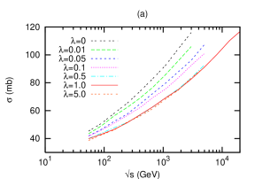
Figure 10: The $pp$ cross section for different values of the coefficient $\lambda$. It is seen in (a) that $\sigma$ does not change for $\lambda\gtrsim 0.5$. This can also be seen from (b) which shows the difference in the cross section, $\Delta\sigma(\lambda)\equiv\sigma(\lambda=0)-\sigma(\lambda)$,as a function of $\lambda$, and for different $s$.

Clearly if $\lambda$ in (8) is very large, the evolution is swamped by recouplings back and forth, making the simulation very inefficient. In this way we also see that the effect of the recouplings must saturate at large enough $\lambda$. By chance it turns out that a value of $\lambda=1$ is just large enough for saturation, see figure 10.

It can be shown that two dipoles recoupling back and forth in this saturated way and colliding with a single dipole according to (2) corresponds exactly to a quadrupole–dipole scattering. Also higher multipole–multipole scatterings are in this way well approximated.

As discussed above these recouplings in some sense also give rise to pomeron mergings, as configurations where one dipole is very small is favored and this dipole has a smaller probability to interact with the target. In our program it is also possible to include explicit mergings of neighboring dipoles, a process which is necessary for the study of exclusive final states and will be studied in a future publication. It should be noted that the combined process of first splitting a dipole into two, then recoupling with a third dipole and finally merging one of them again, corresponds to the recoupling of two dipoles with different colour indices by the exchange of a gluon.

7 Results

In this section we compare results obtained from our model with experimental data from DIS at HERA and $pp$ collisions at the Tevatron. As we yet have not a full control over the virtual dipoles we only study the total cross sections.

7.1 DIS

In [20] we obtained a reasonable qualitative agreement with HERA data for the $F_{2}$ structure function and the effective slope $\lambda_{\mathrm{eff}}(Q^{2})=d(\log F_{2})/d(\log 1/x)$. Having now improved our model further, we will see that we also obtain a good quantitative agreement with the data.

The $\gamma^{*}p$ total cross section is given by the sum of the two wave functions in (13), convoluted with the dipole–proton cross section, $\sigma(z,\boldsymbol{r})$,

$$\sigma_{\gamma^{*}p}^{tot}=\int d^{2}\boldsymbol{r}\int_{0}^{1}dz\{|\psi_{L}(z,r)|^{2}+|\psi_{T}(z,r)|^{2}\}\sigma(z,\boldsymbol{r}).$$ (15)

Here the dipole–proton cross section $\sigma(z,\boldsymbol{r})$ is obtained from equations (5) and by (2), when the initial proton state in section 5 is evolved as described in section 6.

Figure 11: (a) The $\gamma^{*}p$ total cross section shown for different $Q^{2}$. The solid lines include the dipole swing mechanism while the dashed lines do not. $W$ denotes the cms energy. (b) The effective slope measured at different $Q^{2}$. The lines are the same as in (a). Filled circles are data from ZEUS[60] while filled[61] and open[62] squares are data from H1.

In figure 11a we show the results for the $\gamma^{*}p$ total cross section. As we can see the results are in quite good agreement with data except for the fact that the normalization is around 10–15% too high for $Q^{2}\lesssim$ 15 GeV² while it is around 5–10% too high for $Q^{2}\gtrsim$ 45 GeV². Data points are taken from [61, 60] and we also see that the effects of dipole swings are quite small, mainly visible for $Q^{2}\lesssim$ 15 GeV².

As seen from figure 11a, our results seems to have the correct $W$ dependence. This can be seen more clearly from figure 11b, where we show the results for the logarithmic slope $\lambda_{\mathrm{eff}}=d(\log\sigma)/d(\log 1/x)$. We see that there is a good agreement with data for all points lying in the interval 1GeV${}^{2}\lesssim Q^{2}\lesssim$100 GeV². Here the slope is determined within the same energy interval from which the experimental points, taken from [60, 61, 62], are determined.

7.2 Proton–Proton Collisions

Figure 12: The total cross section for $pp$ scattering as a function of the cms energy $\sqrt{s}$. Here results are shown for evolution with and without the dipole swing mechanism. The results for the one pomeron contribution are also shown. Also shown are the results obtained in the “lab” frame where one of the protons is almost at rest.

Figure 13: The $pp$ impact parameter profile, $(1/2)d\sigma_{tot}/d^{2}b$. The points are results obtained from our Monte Carlo while the line is a two parameter Gaussian fit from ref. [63].

The results obtained for the $pp$ total cross section are presented in fig. 12. Here we see that the dipole swing have a rather large effect, as expected. In the figure we also show the results for the one pomeron cross sections, and one can see the large effects of unitarisation. Our main results are calculated in the center of mass frame, where the colliding protons share the energy equally, but in the figure we also show results obtained in the “lab” frame, where one of the protons carries almost all avaliable energy, while the other one is essentially at rest. Due to the fact that the Monte Carlo simulation becomes very inefficient in such a frame (since the energetic proton has to be boosted to quite high rapidities) we have evaluated $\sigma_{tot}$ only up to $\sqrt{s}\sim 1$ TeV. Although the result is not exactly frame independent we see that the frame dependence is reduced, and now very small.

The final result of this paper concerns the impact parameter dependence of the $pp$ total cross section. The result is shown in figure 13. Here we have plotted $(1/2)d\sigma_{tot}/d^{2}b$ as a function of $b$ and for $\sqrt{s}=1.8$TeV. The result is compared to a two parameter Gaussian fit from ref. [63]. There is a quite good agreement between the results. Our profile is more flat and has a somewhat longer tail, but a Gaussian fit to our result would be very similar to the fit in ref. [63].

8 Conclusions

The QCD description of high-energy scattering is clearly a complicated subject. Although a qualitative description of inclusive cross sections for $\gamma^{*}p$ and $pp$ scatterings can be obtained in eg. the B–JIMWLK formalism, it is difficult to give quantitative predictions, and even more difficult to describe exclusive properties of the final states.

In this paper we have described a model of interacting colour dipoles based on a limited set of fairly simple ingredients:

• The description of the initial-state virtual photon and proton as a (set of) dipole(s).

• Simple dipole splittings by gluon emissions according to the Mueller formalism.

• Energy–momentum conservation in each splitting, which gives a dynamic cutoff for small dipole sizes and introduces non-trivial correlations between neighboring dipoles.

• A mechanism for dipole reconnections (or “swing”) corresponding to the introduction of pomeron loops in the evolution.

• A simple dipole–dipole scattering cross section, exponentiated to include multiple scattering and saturation effects.

Although each ingredient is fairly simple, it is prohibitively difficult to include them all in analytic calculations. However, implementing them in a Monte Carlo simulation program we are able to reproduce to a satisfactory degree both the $\gamma^{*}p$ cross sections as measured at HERA as well as the total $pp$ cross section all the way from ISR energies to the Tevatron and beyond. It should be pointed out that this is achieved with effectively only two tuneable parameters, the basic QCD scale $\Lambda_{\mbox{\scriptsize QCD}}$ and $r_{\max}$ giving the non-perturbative cutoff for large dipoles. There are two additional parameters involved in the dipole swing. One is $\lambda$ and we have shown that as long as it is large enough to saturate the recouplings, the results are completely insensitive to this parameter. The other parameter is the number of colour indices, $N_{c}^{2}-1$, which we have fixed to 8, but could in principle be considered a free parameter to simulate the effect of recouplings between differently coloured dipoles by gluon exchange.

The resulting description is quite insensitive to the Lorentz frame chosen to perform the simulations, which shows that we have a consistent treatment of pomeron loops in the evolution and in the scattering of evolved dipole states.

Recently there has been a lot of activity in the subject of high energy evolution in QCD. Different, and very interesting, models have been proposed which are often based on analytical calculations in some toy limit or at asymptotically high energies. We here want to emphasize the importance of a working Monte Carlo simulation in order to confront QCD with real data at realistic energies.

We have also seen that the way the dipole swing is implemented in our model makes it possible to view the evolution as effectively being driven by more general vertices which give rise to more general pomeron transitions during the evolution. Some ideas with such vertices have recently been presented in [55, 57]. There is still more work to do with regard to explicit frame independence in the dipole model, and it is our intention to further study this problem in future investigations.

Another advantage of our model is that it should be possible to also simulate exclusive properties of the final states. Confronting these with experimental observables will allow us to gain further insight into the QCD evolution at high energies. We will return to this problem in a future publication.

References

- [1] J. R. Andersen Phys. Lett. B639 (2006) 290–293, hep-ph/0602182.
- [2] A. H. Mueller Phys. Lett. B104 (1981) 161–164.
- [3] B. I. Ermolaev and V. S. Fadin JETP Lett. 33 (1981) 269–272.
- [4] A. Bassetto, M. Ciafaloni, G. Marchesini, and A. H. Mueller Nucl. Phys. B207 (1982) 189.
- [5] G. Marchesini and B. R. Webber Nucl. Phys. B238 (1984) 1.
- [6] G. Gustafson Phys. Lett. B175 (1986) 453.
- [7] G. Gustafson and U. Pettersson Nucl. Phys. B306 (1988) 746.
- [8] OPAL Collaboration, G. Abbiendi et al. Eur. Phys. J. C35 (2004) 293–312, hep-ex/0306021.
- [9] L3 Collaboration, P. Achard et al. Phys. Lett. B581 (2004) 19–30, hep-ex/0312026.
- [10] ALEPH Collaboration, S. Schael et al. hep-ex/0604042.
- [11] M. Siebel hep-ex/0505080.
- [12] K. Golec-Biernat and M. Wusthoff Phys. Rev. D59 (1999) 014017, hep-ph/9807513.
- [13] K. Golec-Biernat and M. Wusthoff Phys. Rev. D60 (1999) 114023, hep-ph/9903358.
- [14] A. H. Mueller Nucl. Phys. B415 (1994) 373–385.
- [15] A. H. Mueller and B. Patel Nucl. Phys. B425 (1994) 471–488, hep-ph/9403256.
- [16] A. H. Mueller Nucl. Phys. B437 (1995) 107–126, hep-ph/9408245.
- [17] G. P. Salam Comput. Phys. Commun. 105 (1997) 62–76, hep-ph/9601220.
- [18] G. P. Salam Nucl. Phys. B461 (1996) 512–538, hep-ph/9509353.
- [19] E. Avsar hep-ph/0406150.
- [20] E. Avsar, G. Gustafson, and L. Lönnblad JHEP 07 (2005) 062, hep-ph/0503181.
- [21] G. Cohen-Tannoudji, A. Mantrach, H. Navelet, and R. Peschanski Phys. Rev. D28 (1983) 1628.
- [22] A. H. Mueller and H. Navelet Nucl. Phys. B282 (1987) 727.
- [23] L. V. Gribov, E. M. Levin, and M. G. Ryskin Phys. Rept. 100 (1983) 1–150.
- [24] A. Capella, U. Sukhatme, C.-I. Tan, and J. Tran Thanh Van Phys. Rept. 236 (1994) 225–329.
- [25] CDF Collaboration, R. Field Acta Phys. Polon. B36 (2005) 167–178.
- [26] T. Sjostrand and M. van Zijl Phys. Rev. D36 (1987) 2019.
- [27] B. Andersson, G. Gustafson, G. Ingelman, and T. Sjostrand Phys. Rept. 97 (1983) 31.
- [28] B. Andersson, G. Gustafson, and C. Sjogren Nucl. Phys. B380 (1992) 391–407.
- [29] G. Corcella et al. JHEP 01 (2001) 010, hep-ph/0011363.
- [30] T. Sjostrand, S. Mrenna, and P. Skands JHEP 05 (2006) 026, hep-ph/0603175.
- [31] L. Lönnblad Comput. Phys. Commun. 71 (1992) 15–31.
- [32] S. Catani, F. Fiorani, and G. Marchesini Phys. Lett. B234 (1990) 339.
- [33] M. Ciafaloni Nucl. Phys. B296 (1988) 49.
- [34] B. Andersson, G. Gustafson, and J. Samuelsson Nucl. Phys. B467 (1996) 443–478.
- [35] H. Jung and G. P. Salam Eur. Phys. J. C19 (2001) 351–360, hep-ph/0012143.
- [36] H. Jung Comput. Phys. Commun. 143 (2002) 100–111, hep-ph/0109102.
- [37] H. Kharraziha and L. Lönnblad JHEP 03 (1998) 006, hep-ph/9709424.
- [38] H. Kharraziha and L. Lönnblad Comput. Phys. Commun. 123 (1999) 153.
- [39] Y. V. Kovchegov Phys. Rev. D60 (1999) 034008, hep-ph/9901281.
- [40] I. Balitsky Nucl. Phys. B463 (1996) 99–160, hep-ph/9509348.
- [41] E. Iancu, A. Leonidov, and L. McLerran hep-ph/0202270.
- [42] E. Iancu and R. Venugopalan hep-ph/0303204.
- [43] H. Weigert Prog. Part. Nucl. Phys. 55 (2005) 461–565, hep-ph/0501087.
- [44] J. Jalilian-Marian, A. Kovner, A. Leonidov, and H. Weigert Nucl. Phys. B504 (1997) 415–431, hep-ph/9701284.
- [45] J. Jalilian-Marian, A. Kovner, A. Leonidov, and H. Weigert Phys. Rev. D59 (1999) 014014, hep-ph/9706377.
- [46] E. Iancu, A. Leonidov, and L. D. McLerran Phys. Lett. B510 (2001) 133–144, hep-ph/0102009.
- [47] H. Weigert Nucl. Phys. A703 (2002) 823–860, hep-ph/0004044.
- [48] A. H. Mueller and G. P. Salam Nucl. Phys. B475 (1996) 293–320, hep-ph/9605302.
- [49] E. Iancu, A. H. Mueller, and S. Munier Phys. Lett. B606 (2005) 342–350, hep-ph/0410018.
- [50] E. Iancu and A. H. Mueller Nucl. Phys. A730 (2004) 494–513, hep-ph/0309276.
- [51] E. Iancu and D. N. Triantafyllopoulos Nucl. Phys. A756 (2005) 419–467, hep-ph/0411405.
- [52] A. H. Mueller, A. I. Shoshi, and S. M. H. Wong Nucl. Phys. B715 (2005) 440–460, hep-ph/0501088.
- [53] E. Iancu, G. Soyez, and D. N. Triantafyllopoulos Nucl. Phys. A768 (2006) 194–221, hep-ph/0510094.
- [54] E. Levin and M. Lublinsky Nucl. Phys. A763 (2005) 172–196, hep-ph/0501173.
- [55] M. Kozlov, E. Levin, and A. Prygarin hep-ph/0606260.
- [56] A. Kovner and M. Lublinsky Nucl. Phys. A767 (2006) 171–188, hep-ph/0510047.
- [57] J. P. Blaizot, E. Iancu, and D. N. Triantafyllopoulos hep-ph/0606253.
- [58] M. Praszalowicz and A. Rostworowski Acta Phys. Polon. B29 (1998) 745–753, hep-ph/9712313.
- [59] L. Lönnblad Z. Phys. C65 (1995) 285–292.
- [60] ZEUS Collaboration, J. Breitweg et al. Phys. Lett. B487 (2000) 53–73, hep-ex/0005018.
- [61] H1 Collaboration, C. Adloff et al. Eur. Phys. J. C21 (2001) 33–61, hep-ex/0012053.
- [62] A. Petrukhin, “New Measurement of the Structure Function at low with Initial State Radiation Data.” Proceedings of DIS04, Štrbské Pleso, Slovakia, 2004.
- [63] S. Sapeta and K. Golec-Biernat Phys. Lett. B613 (2005) 154–161, hep-ph/0502229.