Mixed Dark Matter in Universal Extra Dimension Models with TeV Scale $W_{\mbox{\tiny R}}$ and $Z^{\prime}$

Abstract:

We show that in a class of universal extra dimension (UED) models that solves both the neutrino mass and proton decay problems using low scale left-right symmetry, the dark matter of the Universe consists of an admixture of KK photon and KK right-handed neutrinos. We present a full calculation of the dark matter density in these models taking into account the co-annihilation effects due to near by states such as the scalar partner of the KK photon as well as fermion states near the right-handed KK neutrino. Using the value of the relic CDM density, we obtain upper limits on $R^{-1}$ of about $400-650$ GeV and $M_{Z^{\prime}}\leq 1.5$ TeV, both being accessible to LHC. For a region in this parameter space where the KK right-handed neutrino contributes significantly to the total relic density of dark matter, we obtain a lower bound on the dark matter-nucleon scattering cross section of $10^{-44}$ cm², which can be probed by the next round of dark matter search experiments.

1 Introduction

Understanding the dark constituent of the Universe is one of the major problems of physics beyond the Standard Model (SM). While in the supersymmetric extensions of the Standard Model, the lightest supersymmetric partner (LSP) of the standard model fields is one of the most well motivated candidates for the cold dark matter (CDM), it is by no means unique and other viable CDM candidates have been proposed in the literature [1, 2, 3]. It is hoped that the Large Hadron Collider (LHC) will provide evidence for supersymmetry making the case for this particle stronger. Nonetheless, at this point, different candidates must be studied in order to isolate their possibly different signatures in other experiments in order to make a proper identification of the true candidate. With this goal in mind, in this paper, we continue our study [4] of a class of dark matter candidates [1, 5], which arises in models with extra dimensions[6, 7, 8], the so-called universal extra dimensional (UED) models [9].

The UED models lead to a very different kind of TeV scale physics and will also be explored at LHC. These models have hidden extra spatial dimensions with sizes of order of an inverse TeV with all SM fields residing in all the dimensions. There could be one or two such extra dimensions and they are compactified with radius $R^{-1}\leq$ TeV [9]. It has recently been pointed out [1] that the lightest Kaluza-Klein (KK) particles of these models being stable can serve as viable dark matter candidates. This result is nontrivial due to the fact that the dark matter relic abundance is determined by the interactions in the theory which are predetermined by the Standard Model. It turns out that in the minimal, 5D extra dimension UED models based on the standard model gauge group, the first KK mode of the hypercharge boson is the dark matter candidate provided the inverse size of the extra dimension is less than a TeV [1].

A generic phenomenological problem with 5D UED models based on the Standard Model gauge group is that they can lead to rapid proton decay as well as unsuppressed neutrino masses. One way to cure the rapid proton decay problem is to consider six dimensions [10] where the two extra spatial dimensions lead to a new $U(1)$ global symmetry that suppresses the strength of all baryon number nonconserving operators. On the other hand both the neutrino mass and the proton decay problem can be solved simultaneously if we extend the gauge group of the six dimensional model to $SU(2)_{L}\times SU(2)_{\mbox{\tiny R}}\times U(1)_{B-L}$ [11]. This avoids having to invoke a seventh warped extra dimension solely for the purpose of solving the neutrino mass problem [12]. With appropriate orbifolding, a neutrino mass comes out to be of the desired order due to a combination two factors: the existence of $B-L$ gauge symmetry and the orbifolding that keeps the left-handed singlet neutrino as a zero-mode which forbids the lower dimensional operators that could give unsuppressed neutrino mass. Another advantage of the 6D models over the 5D ones is that cancellation of gravitational anomaly automatically leads to the existence of the right-handed neutrinos [13] needed for generating neutrino masses.

In a recent paper [4], we pointed out that the 6D UED models with an extended gauge group [11] provide a two-component picture of dark matter consisting of a KK right-handed neutrino and a KK hypercharge boson. We presented a detailed calculation of the relic abundance of both the $\nu^{\mbox{\tiny KK}}_{\mbox{\scriptsize R}}$ and the $B_{Y}^{\mbox{\tiny KK}}$ as well as the cross section for scattering of the dark matter in the cryogenic detectors in these models. The two main results of this calculation[4] are that: (i) present experimental limits on the value of the relic density [14] imply very stringent limits on the the two fundamental parameters of the theory i.e. $R^{-1}$ and the second $Z^{\prime}$-boson associated with the extended gauge group i.e. $R^{-1}\leq 550$ GeV and $M_{Z^{\prime}}\leq 1.2$ TeV and (ii) for one particular region in this parameter range where the relic density of the KK right-handed neutrino contributes significantly to the total relic density of the dark matter, the DM-nucleon cross-section is greater than $10^{-44}$ cm², and is accessible to the next round of dark matter searches. Thus combined with LHC results for an extra $Z^{\prime}$ search, the direct dark matter search experiments could rule out this model. This result is to be contrasted with that of minimal 5-D UED models, where the above experiments will only rule out a part of the parameter space. Discovery of two components to dark matter should also have implications for cosmology of structure formation.

In this paper, we extend the work of ref. [4] in several ways: (i) we update our calculations taking into account the co-annihilation effect of nearby states; (ii) a feature unique to six and higher dimensional models is the presence of physical scalar KK states of gauge bosons degenerate at the tree level with $\gamma_{\mbox{\tiny KK}}$ state and will therefore impact the discussion of KK dark matter. Its couplings to matter have different Lorentz structure and therefore contribute in different ways to the relic density. We discuss the relative significance of the scalar state and its effect on the relic density calculation of the previous paper [4] for both the cases when it is lighter and heavier than the $\gamma_{\mbox{\tiny KK}}$ state. (iii) We also comment on the extra $W$ and $Z^{\prime}$ boson phenomenology in the model.

This paper is organized as follows: in Section 2, we review the basic set up of the model [11]. In Section 3, we present the spectrum of states at tree level. In Sections 4 and 5, we discuss the relic density of $\nu_{KK}$ states and the hypercharge vector and pseudoscalar, respectively. In Section 6, we give the overall picture of dark matter in these models in terms of relic abundance and rates of direct detection. Section 7 discusses the signals such two-component dark matter would give in direct detection experiments. In Section 8, we give the phenomenology of the model for colliders, especially the $Z^{\prime}$ and $W_{\mbox{\tiny R}}$ production and decays. Finally, in Section 9 we present our conclusions.

2 Set up of the Model

We choose the gauge group of the model to be $SU(3)_{c}\times SU(2)_{L}\times SU(2)_{\mbox{\tiny R}}\times U(1)_{\mbox{\tiny B-L}}$ with matter content per generation as follows:

$${\cal Q}_{1,-},{\cal Q}^{\prime}_{1,-}=(3,2,1,\tfrac{1}{3}); {\cal Q}_{2,+},{\cal Q}^{\prime}_{2,+}=(3,1,2,\tfrac{1}{3});$$

$${\cal\psi}_{1,-},{\cal\psi}^{\prime}_{1,-}=(1,2,1,-1); {\cal\psi}_{2,+},{\cal\psi}^{\prime}_{2,+}=(1,1,2,-1);$$ (1)

where, within parenthesis, we have written the quantum numbers that correspond to each group factor, respectively and the subscript gives the six dimensional chirality to cancel gravitational anomaly in six dimensions. We denote the gauge bosons as $G_{M}$, $W^{\pm}_{1,M}$, $W^{\pm}_{2,M}$, and $B_{M}$, for $SU(3)_{c}$, $SU(2)_{L}$, $SU(2)_{\mbox{\tiny R}}$ and $U(1)_{\mbox{\tiny B-L}}$ respectively, where $M=0,1,2,3,4,5$ denotes the six space-time indices. We will also use the following short hand notations: Greek letters $\mu,\nu,\dots=0,1,2,3$ to denote usual four dimensions indices, as usual, and lower case Latin letters $a,b,\dots=4,5$ for those of the extra space dimensions. We will also use $\vec{y}$ to denote the ($x_{4},x_{5}$) coordinates of a point in the extra space.

First, we compactify the extra $x_{4}$, $x_{5}$ dimensions into a torus, $T^{2}$, with equal radii, $R$, by imposing periodicity conditions, $\varphi(x_{4},x_{5})=\varphi(x_{4}+2\pi R,x_{5})=\varphi(x_{4},x_{5}+2\pi R)$ for any field $\varphi$. This has the effect of breaking the original $SO(1,5)$ Lorentz symmetry group of the six dimensional space into the subgroup $SO(1,3)\times Z_{4}$, where the last factor corresponds to the group of discrete rotations in the $x_{4}$-$x_{5}$ plane, by angles of $k\pi/2$ for $k=0,1,2,3$. This is a subgroup of the continuous $U(1)_{45}$ rotational symmetry contained in $SO(1,5)$. The remaining $SO(1,3)$ symmetry gives the usual 4D Lorentz invariance. The presence of the surviving $Z_{4}$ symmetry leads to suppression of proton decay [10] as well as neutrino mass [11].
Employing the further orbifolding conditions :

$$Z_{2} : {\bf{y}}\rightarrow-{\bf{y}}$$ (2)

$$Z^{\prime}_{2} : \left\{\begin{array}[]{ll}(x_{4},x_{5})~{}^{\prime}\rightarrow-(x_{4},x_{5})~{}^{\prime}\\ {\bf{y}}~{}^{\prime}={\bf{y}}-(\pi R/2,\pi R/2)&\end{array}\right.$$ (5)

We can project out the zero modes and obtain the KK modes by assigning appropriate $Z_{2}\times Z^{\prime}_{2}$ quantum numbers to the fields.

In the effective 4D theory the mass of each mode has the form: $m_{N}^{2}=m_{0}^{2}+\frac{N}{R^{2}}$; with $N=\vec{n}^{2}=n_{1}^{2}+n_{2}^{2}$ and $m_{0}$ is the Higgs vacuum expectation value (vev) contribution to mass, and the physical mass of the zero mode.

We assign the following $Z_{2}\times Z^{\prime}_{2}$ charges to the various fields:

$$G_{\mu}(+,+);\ B_{\mu}(+,+);\ W_{1,\mu}^{3,\pm}(+,+);\ W^{3}_{2,\mu}(+,+);\ W^{\pm}_{2,\mu}(+,-);$$

$$G_{a}(-,-);\ B_{a}(-,-);\ W_{1,a}^{3,\pm}(-,-);\ W^{3}_{2,a}(-,-);\ W^{\pm}_{2,a}(-,+).$$ (6)

For quarks we choose,

$$Q_{\mbox{\tiny 1L}}\!\equiv\!\left(\begin{array}[]{c}u_{\mbox{\tiny 1L}}(+,+)\\ d_{\mbox{\tiny 1L}}(+,+)\end{array}\right);\ Q^{\prime}_{\mbox{\tiny 1L}}\!\equiv\!\left(\begin{array}[]{c}u^{\prime}_{\mbox{\tiny 1L}}(+,-)\\ d^{\prime}_{\mbox{\tiny 1L}}(+,-)\end{array}\right);\ Q_{\mbox{\tiny 1R}}\!\equiv\!\left(\begin{array}[]{c}u_{\mbox{\tiny 1R}}(-,-)\\ d_{\mbox{\tiny 1R}}(-,-)\end{array}\right);\ Q^{\prime}_{\mbox{\tiny 1R}}\!\equiv\!\left(\begin{array}[]{c}u^{\prime}_{\mbox{\tiny 1R}}(-,+)\\ d^{\prime}_{\mbox{\tiny 1R}}(-,+)\end{array}\right);$$ (15)

$$Q_{\mbox{\tiny 2L}}\!\equiv\!\left(\begin{array}[]{c}u_{\mbox{\tiny 2L}}(-,-)\\ d_{\mbox{\tiny 2L}}(-,+)\end{array}\right);\ Q^{\prime}_{\mbox{\tiny 2L}}\!\equiv\!\left(\begin{array}[]{c}u^{\prime}_{\mbox{\tiny 2L}}(-,+)\\ d^{\prime}_{\mbox{\tiny 2L}}(-,-)\end{array}\right);\ Q_{\mbox{\tiny 2R}}\!\equiv\!\left(\begin{array}[]{c}u_{\mbox{\tiny 2R}}(+,+)\\ d_{\mbox{\tiny 2R}}(+,-)\end{array}\right);\ Q^{\prime}_{\mbox{\tiny 2R}}\!\equiv\!\left(\begin{array}[]{c}u^{\prime}_{\mbox{\tiny 2R}}(+,-)\\ d^{\prime}_{\mbox{\tiny 2R}}(+,+)\end{array}\right);$$ (24)

and for leptons:

$$\psi_{\mbox{\tiny 1L}} \!\equiv\!\left(\begin{array}[]{c}\nu_{\mbox{\tiny 1L}}(+,+)\\ e_{\mbox{\tiny 1L}}(+,+)\end{array}\right);\ \ \psi^{\prime}_{\mbox{\tiny 1L}}\!\equiv\!\left(\begin{array}[]{c}\nu^{\prime}_{\mbox{\tiny 1L}}(-,+)\\ e^{\prime}_{\mbox{\tiny 1L}}(-,+)\end{array}\right);\ \ \psi_{\mbox{\tiny 1R}}\!\equiv\!\left(\begin{array}[]{c}\nu_{\mbox{\tiny 1R}}(-,-)\\ e_{\mbox{\tiny 1R}}(-,-)\end{array}\right);\ \ \psi^{\prime}_{\mbox{\tiny 1R}}\!\equiv\!\left(\begin{array}[]{c}\nu^{\prime}_{\mbox{\tiny 1R}}(+,-)\\ e^{\prime}_{\mbox{\tiny 1R}}(+,-)\end{array}\right);$$ (33)

$$\psi_{\mbox{\tiny 2L}} \!\equiv\!\left(\begin{array}[]{c}\nu_{\mbox{\tiny 2L}}(-,+)\\ e_{\mbox{\tiny 2L}}(-,-)\end{array}\right);\ \ \psi^{\prime}_{\mbox{\tiny 2L}}\!\equiv\!\left(\begin{array}[]{c}\nu^{\prime}_{\mbox{\tiny 2L}}(+,+)\\ e^{\prime}_{\mbox{\tiny 2L}}(+,-)\end{array}\right);\ \ \psi_{\mbox{\tiny 2R}}\!\equiv\!\left(\begin{array}[]{c}\nu_{\mbox{\tiny 2R}}(+,-)\\ e_{\mbox{\tiny 2R}}(+,+)\end{array}\right);\ \ \psi^{\prime}_{\mbox{\tiny 2R}}\!\equiv\!\left(\begin{array}[]{c}\nu^{\prime}_{\mbox{\tiny 2R}}(-,-)\\ e^{\prime}_{\mbox{\tiny 2R}}(-,+)\end{array}\right).$$ (42)

The zero modes i.e. (+,+) fields corresponds to the standard model fields along with an extra singlet neutrino which is left-handed. They will have zero mass prior to gauge symmetry breaking. The singlet neutrino state being a left-handed (instead of right-handed as in the usual case) has important implications for neutrino mass. For example, the conventional Dirac mass term $\bar{L}H\nu_{\mbox{\tiny R}}$ is not present due to the selection rules of the model and Lorentz invariance. Similarly, $L\tilde{H}\nu_{2L}$ is forbidden by gauge invariance as is the operator $(LH)^{2}$. Thus neutrino mass comes only from much higher dimensional terms.

For the Higgs bosons, we choose a bidoublet, which will be needed to give masses to fermions and break the standard model symmetry and and a pair of doublets $\chi_{L,R}$ with the following $Z_{2}\times Z^{\prime}_{2}$ quantum numbers:

$$\phi\equiv\left(\begin{array}[]{cc}\phi^{0}_{u}(+,+)&\phi^{+}_{d}(+,-)\\ \phi^{-}_{u}(+,+)&\phi^{0}_{d}(+,-)\end{array}\right);\quad\chi_{L}\equiv\left(\begin{array}[]{c}\chi^{0}_{L}(-,+)\\ \chi^{-}_{L}(-,+)\end{array}\right);\quad\chi_{\mbox{\tiny R}}\equiv\left(\begin{array}[]{c}\chi^{0}_{\mbox{\tiny R}}(+,+)\\ \chi^{-}_{\mbox{\tiny R}}(+,-)\end{array}\right),$$ (49)

and the following charge assignment under the gauge group,

$$\phi = (1,2,2,0),$$

$$\chi_{L} = (1,2,1,-1),\quad\chi_{\mbox{\tiny R}}=(1,1,2,-1).$$ (50)

At the zero mode level, only the SM doublet $(\phi^{0}_{u},\phi^{-}_{u})$ and a singlet $\chi^{0}_{\mbox{\tiny R}}$ appear. The vacuum expectation values (vev) of these fields, namely $\langle\phi^{0}_{u}\rangle=v_{wk}$ and $\langle\chi^{0}_{\mbox{\tiny R}}\rangle=v_{\mbox{\tiny R}}$, break the SM symmetry and the extra $U(1)_{Y}^{\prime}$ gauge group, respectively. A diagram that illustrates the lowest KK modes of all the particles and their masses is shown in Fig. 1 with the following identification of modes in Table 1.

($Z_{2},Z_{2}^{\prime}$)	Particle Content
(++)	$\begin{array}[]{l}Q_{\mbox{\tiny 1L}};~{}u_{\mbox{\tiny 2R}};~{}d^{\prime}_{\mbox{\tiny 2R}};~{}\psi_{\mbox{\tiny 1L}};~{}e_{\mbox{\tiny 2R}};~{}\nu^{\prime}_{\mbox{\tiny 2L}};\vspace{0.05in}\\ G_{\mu};~{}B_{\mu};~{}W_{1,\mu}^{3,\pm};~{}W_{2,\mu}^{3};\vspace{0.05in}\\ \phi_{u}^{0};~{}\phi_{u}^{-};~{}\chi_{\mbox{\tiny R}}^{\mbox{\tiny 0}}\vspace{0.05in}\end{array}$
($+-$)	$\begin{array}[]{l}Q^{\prime}_{\mbox{\tiny 1L}};~{}u^{\prime}_{\mbox{\tiny 2R}};~{}d_{\mbox{\tiny 2R}};~{}\psi^{\prime}_{\mbox{\tiny 1R}};~{}\nu_{\mbox{\tiny 2R}};~{}e^{\prime}_{\mbox{\tiny 2R}};\vspace{0.05in}\\ W_{2,\mu}^{\pm};\vspace{0.05in}\\ \phi_{d}^{+};~{}\phi_{d}^{\mbox{\tiny 0}};~{}\chi_{\mbox{\tiny R}}^{\mbox{\tiny-}}\vspace{0.05in}\end{array}$
($-+$)	$\begin{array}[]{l}Q^{\prime}_{\mbox{\tiny 1R}};~{}u^{\prime}_{\mbox{\tiny 2L}};~{}d_{\mbox{\tiny 2L}};~{}\psi^{\prime}_{\mbox{\tiny 1L}};~{}\nu_{\mbox{\tiny 2L}};~{}e^{\prime}_{\mbox{\tiny 2R}};\vspace{0.05in}\\ W_{2,a}^{\pm};\vspace{0.05in}\\ \chi_{\mbox{\tiny L}}^{\mbox{\tiny 0}};~{}\chi_{\mbox{\tiny L}}^{\mbox{\tiny-}}\vspace{0.05in}\end{array}$
($--$)	$\begin{array}[]{l}Q_{\mbox{\tiny 1R}};~{}u_{\mbox{\tiny 2L}};~{}d^{\prime}_{\mbox{\tiny 2L}};~{}\psi_{\mbox{\tiny 1R}};~{}\nu_{\mbox{\tiny 1R}};~{}e_{\mbox{\tiny 2L}};\vspace{0.05in}\\ G_{a};~{}B_{a};~{}W_{1,a}^{3,\pm};~{}W_{2,a}^{3}\vspace{0.05in}\end{array}$

Table 1: Particle content of 6D model separated by $Z_{2}\times Z_{2}^{\prime}$ parities.

Figure 1: The masses of lowest KK-modes of 6D model.

The most general Yukawa couplings in the model are

$$h_{u}\bar{Q}_{1}\phi Q_{2}+h_{d}\bar{Q}_{1}\tilde{\phi}Q^{\prime}_{2}+h_{e}\bar{\psi}_{1}\tilde{\phi}\psi_{2}+h^{\prime}_{u}\bar{Q}^{\prime}_{1}\phi Q^{\prime}_{2}+h^{\prime}_{d}\bar{Q}^{\prime}_{1}\tilde{\phi}Q_{2}+h^{\prime}_{e}\bar{\psi}^{\prime}_{1}\tilde{\phi}\psi^{\prime}_{2}+h.c.;$$ (51)

where $\tilde{\phi}\equiv\tau_{2}\phi^{*}\tau_{2}$ is the charge conjugate field of $\phi$. A six dimensional realization of the left-right symmetry, which interchanges the subscripts: $1\leftrightarrow 2$, is obtained provided the $3\times 3$ Yukawa coupling matrices satisfy the constraints: $h_{u}~{}=~{}h^{\dagger}_{u}$; $h^{\prime}_{u}~{}=~{}h^{{}^{\prime}\dagger}_{u}$; $h_{e}~{}=~{}h^{\dagger}_{e};$ $h^{\prime}_{e}~{}=~{}h^{{}^{\prime}\dagger}_{e};$ $h_{d}~{}=~{}h^{{}^{\prime}\dagger}_{d}$. At the zero mode level one obtains the SM Yukawa couplings

$${\cal L}~{}=~{}h_{u}\bar{Q}\phi_{u}u_{R}+h_{d}\bar{Q}\tilde{\phi}_{u}d_{R}+h_{e}\bar{L}\tilde{\phi}_{u}e_{R}+h.c.$$ (52)

It is important to notice that in the above equation $h_{u,e}$ are hermitian matrices, while $h_{d}$ is not. The vev of $\phi_{u}$ gives mass to the charged fermions of the model. As far as the neutrino mass is concerned, the lowest dimensional gauge invariant operator in six-D that gives rise to neutrino mass after compactificaion has the form $\psi^{T}_{1,L}{\phi}\psi_{2,L}\chi^{2}_{R}$ and leads to neutrino mass $m_{\nu}\simeq\lambda\frac{v_{wk}v^{2}_{R}}{M^{2}_{*}(M^{2}_{*}R)^{3}}$. For $M_{*}R\sim 100$ and $M_{*}\sim$ 10 TeV, $v_{R}\sim 2$ TeV and $\lambda\sim 10^{-3}$, we get neutrino masses of order $\sim$ eV without fine tuning. Furthermore, it predicts that the neutrino mass is Dirac (predominantly) rather than Majorana type.

As there are a large number of KK modes, one may worry whether or not electroweak precision constraints in terms of S and T parameters are satisfied. It has been shown that in the minimal universal extra dimension (MUED) the KK contributions to the T parameter almost cancel for heavier standard model Higgs [9, 15]. However, it was found that in the MUED for Higgs mass heavier than 300 GeV the lightest Kaluza-Klein particle is the charged KK Higgs [16]. The abundance of such charged massive particles are inconsistent with big bang nucleosynthesis as well as other cosmological observations for masses less than a TeV [17]. This lead to the conclusion that the compactification scale $1/R>$ 400 GeV for $m_{H}>$ 300 GeV. To our knowledge, there has been no such analysis for the $6-$D models similar to ours, and it is outside the scope of the current paper to perform a complete analysis regarding the electroweak constraints. Therefore, we leave the investigation of this open issue for future work.

3 Spectrum of Particles

Once the extra dimensions are compactified, the KK modes are labelled by the quanta of momenta in the extra dimensions. As we have two such extra spatial dimensions, the KK modes are labelled by two integers, and we will denote a KK mode as $\phi^{(mn)}$, where $m$ ($n$) is the momentum in the quantized unit of $R^{-1}$ along the fifth (sixth) dimension. A detailed expansion of a field in the 6D theory into KK mode is presented in the Appendix. Generally, $\phi^{(mn)}$ would receive a (mass)² of the order $(m^{2}+n^{2})R^{-2}$.

3.1 Gauge and Higgs Particles at the Zeroth KK Level

In the gauge basis, we have the zero-mode gauge bosons: $B^{\mbox{\scriptsize(00)}}_{\mbox{\tiny(B-L)}\mu},W^{\pm,3\mbox{\scriptsize(00)}}_{L,\mu}$, and $W^{3\mbox{\scriptsize(00)}}_{R,\mu}$. After symmetry-breaking, we will have the usual SM gauge bosons: one exactly massless gauge boson, $A_{\mu}^{\mbox{\scriptsize(00)}}$, one pair of massive, charged vector boson $W_{L,\mu}^{\pm,\mbox{\scriptsize(00)}}$, and one massive neutral guage boson $Z_{\mu}^{\mbox{\scriptsize(00)}}$. In addition, we will have another neutral gauge boson $Z_{\mu}^{\prime\mbox{\scriptsize(00)}}$, as well as mixing between $Z_{\mu}^{\mbox{\scriptsize(00)}}$ and $Z_{\mu}^{\prime\mbox{\scriptsize(00)}}$.

In this subsection we calculate the zeroth-mode gauge boson masses and mixings from Higgs mechanism (and drop the $(00)$ superscript throughout this subsection). The relevant terms are

$$\mathcal{L}_{h}=\mbox{Tr}[(D_{\mu}\phi)^{{\dagger}}D_{\mu}\phi]+(D^{\mu}\chi_{\mbox{\tiny R}})^{\ast}D_{\mu}\chi_{\mbox{\tiny R}}+(D^{\mu}\chi_{L})^{\ast}D_{\mu}\chi_{L}$$ (53)

where

$$D_{\mu}\phi =\partial_{\mu}\phi-ig_{\mbox{\tiny{L}}}(\overrightarrow{\tau}\cdot\overrightarrow{W_{L}}_{\mu})\phi+ig_{\mbox{\tiny{R}}}\phi(\overrightarrow{\tau}\cdot\overrightarrow{W_{\mbox{\tiny R}}}_{\mu}),$$

$$\phi =\begin{pmatrix}\phi_{u}^{0}&\phi_{d}^{+}\\ \phi_{u}^{-}&\phi_{d}^{0}\end{pmatrix},$$

$$D_{\mu}\chi_{L} =\left(\partial_{\mu}-ig_{\mbox{\tiny{L}}}(\overrightarrow{\tau}\cdot\overrightarrow{W_{L},}_{\mu})+i(\frac{1}{2})g_{\mbox{\tiny{BL}}}B_{\mbox{\tiny(B-L)},\mu}\right)\begin{pmatrix}\chi_{L}^{0}\\ \chi_{L}^{-}\end{pmatrix},$$

$$D_{\mu}\chi_{\mbox{\tiny R}} =\left(\partial_{\mu}-ig_{\mbox{\tiny{R}}}(\overrightarrow{\tau}\cdot\overrightarrow{W_{\mbox{\tiny R}},}_{\mu})+i(\frac{1}{2})g_{\mbox{\tiny{BL}}}B_{\mbox{\tiny(B-L)},\mu}\right)\begin{pmatrix}\chi_{\mbox{\tiny R}}^{0}\\ \chi_{\mbox{\tiny R}}^{-}\end{pmatrix},$$

$$\overrightarrow{\tau}\cdot\overrightarrow{W_{\mu}} =\frac{1}{2}\begin{pmatrix}W^{3}_{\mu}&\sqrt{2}W_{\mu}^{+}\\ \sqrt{2}W_{\mu}^{-}&-W^{3}_{\mu}\end{pmatrix}.$$ (54)

With vev of the fields $\langle\phi_{u}^{0}\rangle=v_{w}$ and $\langle\chi_{\mbox{\tiny R}}^{0}\rangle=v_{\mbox{\tiny R}}$, we obtain the following mass terms for the gauge bosons:

$$\mathcal{L} =\frac{1}{2}v^{2}_{w}(W^{+}_{L,\mu}W^{-}_{L,\mu})+\frac{1}{2}(v^{2}_{w}+v^{2}_{\mbox{\tiny R}})(W^{+}_{R,\mu}W^{-}_{R,\mu})$$

$$+\frac{1}{2}\begin{pmatrix}W^{3}_{L,{\mu}}&W^{3}_{R,{\mu}}&B_{\mbox{\tiny(B-L)}\mu}\end{pmatrix}\begin{pmatrix}\frac{1}{2}g_{\mbox{\tiny{L}}}^{2}v_{w}^{2}&-\frac{1}{2}g_{\mbox{\tiny{L}}}g_{\mbox{\tiny{R}}}v_{w}^{2}&0\\ -\frac{1}{2}g_{\mbox{\tiny{L}}}g_{\mbox{\tiny{R}}}v_{w}^{2}&\frac{1}{2}g_{\mbox{\tiny{R}}}^{2}(v_{w}^{2}+v_{\mbox{\tiny R}}^{2})&-\frac{1}{2}(g_{\mbox{\tiny{R}}}g_{\mbox{\tiny{BL}}})v_{\mbox{\tiny R}}^{2}\\ 0&-\frac{1}{2}(g_{\mbox{\tiny{R}}}g_{\mbox{\tiny{BL}}})v_{\mbox{\tiny R}}^{2}&\frac{1}{2}g_{\mbox{\tiny{BL}}}^{2}v_{\mbox{\tiny R}}^{2}\end{pmatrix}\begin{pmatrix}W^{3,\mu}_{L}\\ W^{3,\mu}_{R}\\ B_{\mbox{\tiny(B-L)}}^{\mu}\end{pmatrix}.$$ (55)

The exact expressions of the mass eigenvalues and the compositions of the eigenstates $(A_{\mu},Z_{\mu},Z^{\prime}_{\mu})$ in terms of $(B_{\mbox{\tiny(B-L)}\mu},W^{3}_{L,\mu},W^{3}_{R,\mu})$ are rather complicated, and we make the approximation of $v_{\mbox{\tiny R}}\gg v_{w}$. In this approximation, we find the relations,

$$\begin{pmatrix}A_{\mu}\\ Z_{\mu}\\ Z^{\prime}_{\mu}\end{pmatrix}=U^{{\dagger}}_{G}\begin{pmatrix}W^{0}_{1,\mu}\\ W^{0}_{2,\mu}\\ B_{\mu}\end{pmatrix},$$ (56)

where

$$U^{{\dagger}}_{G}=\begin{pmatrix}\sin\theta_{w}&\cos\theta_{w}&0\\ \cos\theta_{w}&-\sin\theta_{w}&0\\ 0&0&1\end{pmatrix}\begin{pmatrix}1&0&0\\ 0&\sin\theta_{\mbox{\tiny R}}&\cos\theta_{\mbox{\tiny R}}\\ 0&\cos\theta_{\mbox{\tiny R}}&-\sin\theta_{\mbox{\tiny R}}\end{pmatrix},$$ (57)

and

$$\tan\theta_{\mbox{\tiny R}}\equiv\frac{g_{\mbox{\tiny{BL}}}}{g_{\mbox{\tiny{R}}}},\quad g_{\mbox{\tiny{Y}}}^{2}\equiv\frac{g_{\mbox{\tiny{BL}}}^{2}g_{\mbox{\tiny{R}}}^{2}}{g_{\mbox{\tiny{BL}}}^{2}+g_{\mbox{\tiny{R}}}^{2}},\quad\mbox{and}\quad\tan\theta_{w}\equiv\frac{g_{\mbox{\tiny{Y}}}}{g_{\mbox{\tiny{L}}}}.$$ (58)

It is easy to understand $U_{G}$ intuitively. In the limit $v_{w}\ll v_{\mbox{\tiny R}}$, the symmetry-breaking occurs in two stages, corresponding to the two matrices in $U_{G}$. First, we have $SU(2)_{L}\times SU(2)_{\mbox{\tiny R}}\times U(1)_{\mbox{\tiny B-L}}\rightarrow SU(2)_{L}\times U(1)_{Y}$, where a linear combination of $B_{\mbox{\tiny(B-L)},\mu}$ and $W^{3}_{R,\mu}$ acquire a mass to become $Z_{\mu}^{\prime}$, while the orthogonal combination, $B_{Y,\mu}$, remains massless and serves as the gauge boson of the residual group $U(1)_{Y}$. Then we have the standard electroweak breaking of $SU(2)_{L}\times U(1)_{Y}\rightarrow U(1)_{\mbox{\scriptsize em}}$, giving us massive $Z_{\mu}$ and the massless photon $A_{\mu}$. Using $U_{G}$, we can simplify the mass matrix enormously

$$U^{{\dagger}}_{G}\mathcal{M}^{2}U_{G} =\begin{pmatrix}0&0&0\\ 0&M_{Z}^{2}&-\frac{g_{\mbox{\tiny{R}}}^{2}}{\sqrt{(g_{\mbox{\tiny{L}}}^{2}+g_{\mbox{\tiny{Y}}}^{2})(g_{\mbox{\tiny{R}}}^{2}+g_{\mbox{\tiny{BL}}}^{2})}}M_{Z}^{2}\\ 0&-\frac{g_{\mbox{\tiny{R}}}^{2}}{\sqrt{(g_{\mbox{\tiny{L}}}^{2}+g_{\mbox{\tiny{Y}}}^{2})(g_{\mbox{\tiny{R}}}^{2}+g_{\mbox{\tiny{BL}}}^{2})}}M_{Z}^{2}&M_{Z^{\prime}}^{2}\end{pmatrix},$$ (59)

where we have defined the mass eigenvalues (up to $\mathcal{O}(v_{w}/v_{\mbox{\tiny R}})^{2}$)

$$M_{Z}^{2} =\left(g_{\mbox{\tiny{L}}}^{2}+g_{\mbox{\tiny{Y}}}^{2}\right)\frac{v^{2}_{w}}{2}$$

$$M_{Z^{\prime}}^{2} =(g_{\mbox{\tiny{BL}}}^{2}+g_{\mbox{\tiny{R}}}^{2})\frac{v^{2}_{\mbox{\tiny R}}}{2}+\frac{g_{\mbox{\tiny{R}}}^{4}}{(g_{\mbox{\tiny{BL}}}^{2}+g_{\mbox{\tiny{R}}}^{2})}\frac{v_{w}^{2}}{2}.$$ (60)

Here we see that we have explicitly decoupled $A_{\mu}$, and it remains massless exactly. Although we have defined $M_{Z}$ to be same as the tree-level mass of $Z$-boson of the Standard Model, here $Z_{\mu}$ is strictly speaking not an eigenstate because of the $Z-Z^{\prime}$ mixing. Such mixing would be important, as we will see, for the calculation of relic density and the direct detection rates of the dark matter of the model. However, in the limit $v^{2}_{\mbox{\tiny R}}\gg v^{2}_{w}$ that we will be working with, we can treat the defined masses and states in Eq. 60 as eigenvalues and eigenstates, and treat the mixing terms perturbatively in powers of $(v_{w}^{2}/v_{\mbox{\tiny R}}^{2})$.

The only zero-mode Higgs bosons in the model are $\phi_{u}^{0\mbox{\scriptsize(00)}},\phi_{u}^{-\mbox{\scriptsize(00)}},$ and $\chi_{\mbox{\tiny R}}^{0,\mbox{\scriptsize(00)}}$. Four of the six degrees of freedoms are eaten and the remaining physical Higgs particles are the real parts of $\phi_{u}^{0\mbox{\scriptsize(00)}}$ and $\chi_{\mbox{\tiny R}}^{0,\mbox{\scriptsize(00)}}$. The masses are these particles are determined from the potential, and are free parameters, whose values, however, do not affect the calculations of the relic density and direct detection rates of the dark matter.

3.2 Gauge and Higgs Particles at the First KK Level

We first consider the question of whether KK modes of Higgs bosons acquire vevs. The zero modes Higgs bosons acquire vevs due to negative mass-squared terms in the potential. The higher KK modes of the Higgs bosons $\phi^{\mbox{\scriptsize(mn)}}$, however, have an additional mass-squared contribution of the form $(m^{2}+n^{2})R^{-2}$. Therefore, if the negative mass-squared term in the potential is smaller in magnitude than $R^{-2}$, then none of the higher Higgs KK modes would acquire vevs. We will assume this is the case in our calculations, and the only fields that acquire vevs are $\phi_{u}^{0\mbox{\scriptsize(00)}}$ and $\chi_{\mbox{\tiny R}}^{0,\mbox{\scriptsize(00)}}$, the zero-modes of neutral Higgs fields.

Here we will only consider the details of those gauge bosons in the $(11)$ KK modes, and in this subsection it is understood that we have the superscript $(11)$. That is, we do not consider the $(01)$ and $(10)$ modes of $W^{\pm}_{R,\mu,5,6}$. For a compact notation that will be convenient later on, for the scalar partners ($G_{5}$ and $G_{6}$) of a generic vector gauge boson ($G_{\mu}$), we form the combinations

$$G_{(\pm)}\equiv\frac{1}{\sqrt{2}}(G_{5}\pm G_{6}).$$ (61)

In the absence of Higgs mechanism, $G_{(+)}$ will be eaten by $G_{\mu}$ at the corresponding KK-level, while $G_{(-)}$ will be left as a physical degree of freedom. Qualitatively, $W^{\pm}_{R,\mu}$ eats a linear combination of $W^{\pm}_{R,(+)}$, $W^{\pm}_{R,(-)}$, and $\chi_{\mbox{\tiny R}}^{-}$ (all fields with the superscript $(01)$ and $(10)$), while the two remaining orthogonal directions are left as physical degrees of freedom.

At the $(11)$-level, before symmetry breaking, we have the modes

Neutral Gauge Bosons: $$\quad W^{3}_{L,\mu},W^{3}_{R,\mu},B_{\mu}$$

Neutral Scalars: $$\quad W^{3}_{L,(+)},W^{3}_{L,(-)},W^{3}_{R,(+)},W^{3}_{R,(-)},B_{(+)},B_{(-)},\phi_{u}^{0},\chi_{\mbox{\tiny R}}^{0}$$

Charged Gauge Bosons: $$\quad W^{\pm}_{L\mu}$$

Charged Scalars: $$\quad W^{\pm}_{L,(+)},W^{\pm}_{L,(-)},\phi_{u}^{-}.$$ (62)

Three (two) linear combinations of the neutral (charged) scalars would be eaten, leaving seven (four) degrees of freedom (note that the Higgs fields are complex). Since only the zero-mode Higgs acquire vevs, the Higgs mechanism contribution to the mass matrix of the neutral gauge bosons is same as that in Eq. 55, and we have an additional contribution of $2R^{-2}\mathbf{1}_{3\times 3}$. We can diagonalize the (mass)² matrix up to $\mathcal{O}(v_{w}^{2}/v_{\mbox{\tiny R}}^{2})$ using the same unitary matrix $U_{G}$ and obtain the eigenvalues to be those in Eq. 60 with the additional $2R^{-2}$.

Of the neutral scalars, we have several sets of particles that do not mix with members of other sets at tree level:

Set 1: $$\quad\tfrac{1}{\sqrt{2}}\mbox{Re}[\phi_{u}^{0}],\tfrac{1}{\sqrt{2}}\mbox{Re}[\chi_{\mbox{\tiny R}}^{0}]$$

Set 2: $$\quad W^{3}_{L,(-)},W^{3}_{R,(-)},B_{(-)}$$

Set 3: $$\quad W^{3}_{L,(+)},W^{3}_{R,(+)},B_{(+)},\tfrac{1}{\sqrt{2}}\mbox{Im}[\phi_{u}^{0}],\tfrac{1}{\sqrt{2}}\mbox{Im}[\chi_{\mbox{\tiny R}}^{0}].$$ (63)

The squared-mass of particles in Set 1 are simply $2R^{-2}$ in addition to the squared-masses of corresponding particles at $(00)$-modes. The mass matrix of particles in Set 2 are exactly that of the neutral gauge bosons, with a lightest mode of $A_{(-)}$ with mass $m_{A_{(-)}}=m_{A_{\mu}}=\sqrt{2}R^{-1}$. Three linear combinations of particles in Set 3 are eaten, and the two remaining particles have masses that will depend on the Higgs potential. As is the case with the zeroth-modes, as long as these Higgs are heavier than the lightest gauge bosons, the values of their masses will not affect our results about the dark matter of the model.

3.3 Spectrum of Matter Fields

Because there is no yukawa coupling between the Higgs doublet $\chi_{\mbox{\tiny R}}$ and matter, at tree level all mass terms arise from the momentum in the extra dimensions and $v_{w}$. The structure of the yukawa couplings, with the $Z_{2}\times Z_{2}^{\prime}$ orbifolding ensures that the zero-mode matter fields have the SM spectrum. As for the higher modes, the mass terms arising from the extra dimension connect the left- and right-handed components of a 6D chiral fermion $\Psi_{\pm}$, where $\pm$ denotes 6D chirality. The mass terms arising from electroweak symmetry-breaking, however, connects left- and right-handed components of two different 6D chiral fields. Taking the electron as an example, the mass matrix of the electron KK modes in the basis $\{e_{1L}\ e_{1R}\ e_{2L}\ e_{2R}\}$ (with $e_{1L}$ and $e_{2R}$ having zero modes) is

$$\mathcal{M}_{e^{(1)}} =\begin{pmatrix}\overline{e}_{1L}&\overline{e}_{1R}&\overline{e}_{2L}&\overline{e}_{2R}\end{pmatrix}\begin{pmatrix}0&R^{-1}&0&y_{e}\tfrac{v_{2}}{\sqrt{2}}\\ R^{-1}&0&y_{e}\tfrac{v_{2}}{\sqrt{2}}&0\\ 0&y_{e}\tfrac{v_{2}}{\sqrt{2}}&0&-R^{-1}\\ y_{e}\tfrac{v_{2}}{\sqrt{2}}&0&-R^{-1}&0\end{pmatrix}\begin{pmatrix}e_{1L}\\ e_{1R}\\ e_{2L}\\ e_{2R}\end{pmatrix}$$

$$=\begin{pmatrix}\overline{e}_{1}&\overline{e}_{2}\end{pmatrix}\begin{pmatrix}R^{-1}&y_{e}\tfrac{v_{2}}{\sqrt{2}}\\ y_{e}\tfrac{v_{2}}{\sqrt{2}}&-R^{-1}\end{pmatrix}\begin{pmatrix}e_{1}\\ e_{2}\end{pmatrix}.$$ (64)

Generalizing this, we see that the $(mn)$ modes have masses

$$m_{f^{(mn)}}=\left(\frac{N^{2}}{R^{2}}\pm m^{2}_{f^{(00)}}\right)^{1/2},$$ (65)

where $N^{2}=m^{2}+n^{2}$ and $m^{2}_{f^{(00)}}=y_{f}^{2}\frac{v_{w}^{2}}{2}$ is the zero-mode mass of the fermion.

3.3.1 Possible Dark Matter Candidates

In order to see the dark matter candidates in our model, we look at the spectrum of the KK modes (see Fig. 1). There are two classes of KK modes of interest whose stability is guaranteed by KK parity: the ones with $(-,-)$ and $(\pm,\mp)$ $Z_{2}\times Z^{\prime}_{2}$ quantum numbers. The former have mass $\sqrt{2}R^{-1}$ and the latter $R^{-1}$. We see from Fig. 1 that the first class of particles are the first KK mode of the hypercharge gauge boson $B_{Y}$ and the second are the right handed neutrinos $\nu_{\mbox{\tiny 2L, 2R}}$. The presence of the RH neutrino dark matter makes the model predictive and testable as we will see quantitatively in what follows. The basic idea is that $\nu_{\mbox{\tiny R}}$ annihilation proceeds primarily via the exchange of the $Z^{\prime}$ boson. So as the $Z^{\prime}$ boson mass gets larger, the annihilation rate goes down very fast (like $M^{-4}_{Z^{\prime}}$) and the $\nu_{\mbox{\tiny 2}}$’s overclose the Universe. Also since there are lower limits on the $Z^{\prime}$ mass from collider searches [25], the $\nu_{\mbox{\tiny 2}}$’s contribute a minimum amount to the $\Omega_{\mbox{\tiny DM}}$. This leads to a two-component picture of dark matter and also adds to direct scattering cross section making the dark matter detectable. Below we make these comments more quantitative and present our detailed results.

4 Dark Matter Candidate I: $\nu_{\mbox{\tiny 2L,2R}}$

4.1 Annihilation Channels of $\nu_{\mbox{\tiny 2L,2R}}$

Since the yukawa couplings are small, except for the top-quark coupling, we only consider annihilations through gauge-mediated processes. For completeness, we first list the couplings between matter fields and the neutral vector gauge bosons. For matter fields charged under $SU(2)_{1}$, we have

$$\mathcal{L}^{SU(2)_{1}}_{\overline{f}fB} =(\overline{q}\gamma^{\mu}P_{L}q)\left[\left(T^{3}_{L}+\frac{Y_{BL}}{2}\right)\left(\frac{g_{\mbox{\tiny{L}}}g_{\mbox{\tiny{R}}}g_{\mbox{\tiny{BL}}}}{\sqrt{g_{\mbox{\tiny{L}}}^{2}g_{\mbox{\tiny{R}}}^{2}+g_{\mbox{\tiny{BL}}}^{2}g_{\mbox{\tiny{L}}}^{2}+g_{\mbox{\tiny{BL}}}^{2}g_{\mbox{\tiny{R}}}^{2}}}\right)A_{\mu}\right.$$

$$\quad\qquad\qquad+\left(\frac{T^{3}_{L}g_{\mbox{\tiny{L}}}^{2}(g_{\mbox{\tiny{R}}}^{2}+g_{\mbox{\tiny{BL}}}^{2})-\tfrac{Y_{BL}}{2}g_{\mbox{\tiny{R}}}^{2}g_{\mbox{\tiny{BL}}}^{2}}{\sqrt{g_{\mbox{\tiny{L}}}^{2}g_{\mbox{\tiny{R}}}^{2}+g_{\mbox{\tiny{BL}}}^{2}g_{\mbox{\tiny{L}}}^{2}+g_{\mbox{\tiny{BL}}}^{2}g_{\mbox{\tiny{R}}}^{2}}\sqrt{g_{\mbox{\tiny{BL}}}^{2}+g_{\mbox{\tiny{R}}}^{2}}}\right)Z_{\mu}$$

$$\left.\quad\quad\qquad+\left(\frac{Y_{BL}}{2}\frac{g_{\mbox{\tiny{BL}}}^{2}}{\sqrt{g_{\mbox{\tiny{BL}}}^{2}+g_{\mbox{\tiny{R}}}^{2}}}\right)Z^{\prime}_{\mu}\right].$$ (66)

And for matter fields charged under $SU(2)_{2}$,

$$\mathcal{L}^{SU(2)_{2}}_{\overline{f}fB} =(\overline{q}\gamma^{\mu}P_{\mbox{\tiny R}}q)\left[\left(T^{3}_{R}+\frac{Y_{BL}}{2}\right)\left(\frac{g_{\mbox{\tiny{L}}}g_{\mbox{\tiny{R}}}g_{\mbox{\tiny{BL}}}}{\sqrt{g_{\mbox{\tiny{L}}}^{2}g_{\mbox{\tiny{R}}}^{2}+g_{\mbox{\tiny{BL}}}^{2}g_{\mbox{\tiny{L}}}^{2}+g_{\mbox{\tiny{BL}}}^{2}g_{\mbox{\tiny{R}}}^{2}}}\right)A_{\mu}\right.$$

$$\quad\qquad\qquad+\left(-T^{3}_{R}-\frac{Y_{BL}}{2}\right)\left(\frac{g_{\mbox{\tiny{R}}}^{2}g_{\mbox{\tiny{BL}}}^{2}}{\sqrt{g_{\mbox{\tiny{L}}}^{2}g_{\mbox{\tiny{R}}}^{2}+g_{\mbox{\tiny{BL}}}^{2}g_{\mbox{\tiny{L}}}^{2}+g_{\mbox{\tiny{BL}}}^{2}g_{\mbox{\tiny{R}}}^{2}}\sqrt{g_{\mbox{\tiny{BL}}}^{2}+g_{\mbox{\tiny{R}}}^{2}}}\right)Z_{\mu}$$

$$\left.\quad\qquad\qquad+\left(\frac{-T^{3}_{R}g_{\mbox{\tiny{R}}}^{2}+\tfrac{Y_{BL}}{2}g_{\mbox{\tiny{BL}}}^{2}}{\sqrt{g_{\mbox{\tiny{BL}}}^{2}+g_{\mbox{\tiny{R}}}^{2}}}\right)Z^{\prime}_{\mu}\right],$$ (67)

where $T^{3}_{\mbox{\tiny L}}=\pm\tfrac{1}{2}$ and $T^{3}_{\mbox{\tiny R}}=\pm\tfrac{1}{2}$ are the quantum number for the $SU(2)_{1}$ and $SU(2)_{2}$ groups respectively. We choose this notation because $SU(2)_{1}$ is to be identified with $SU(2)_{L}$ of the Standard Model, even though there are right-handed particles that are charged under the $SU(2)_{1}$ group. Also, $Y_{\mbox{\scriptsize BL}}=+1/3$ for quarks and $Y_{\mbox{\scriptsize BL}}=-1$ for leptons.

Using these formulas, the gauge interaction of the dark matter candidates $\nu_{2L,2R}$ is given by the six-dimensional Lagrangian

$$\mathcal{L}_{\nu} =-\frac{1}{2}(\overline{\nu}\gamma^{\mu}\nu)\frac{g_{\mbox{\tiny{R}}}^{2}+g_{\mbox{\tiny{BL}}}^{2}}{\sqrt{g_{\mbox{\tiny{BL}}}^{2}+g_{\mbox{\tiny{R}}}^{2}}}Z^{\prime}_{\mu}.$$ (68)

We first notice that $\nu_{\mbox{\tiny 2L,2R}}$ couple as a Lorentz vector. Second, we see that $\nu_{\mbox{\tiny 2L,2R}}$ do not couple to $A_{\mu}$ nor $Z_{\mu}$ as expected because $\nu_{\mbox{\tiny 2L,2R}}$ are singlets under the SM gauge group. There is a small coupling between $\nu_{\mbox{\tiny 2L,2R}}$ and $Z_{\mu}$ due to $Z^{\prime}_{\mu}-Z_{\mu}$ mixing. For the purpose of evaluating annihilation cross sections, we can safely ignore this mixing, as we will show. However, this mixing will be important when we consider the direct detection of $\nu_{\mbox{\tiny 2L,2R}}$. In addition, we have the charged-current interaction, similar to the SM case

$$\mathcal{L}_{\mbox{\scriptsize CC}}=\frac{g_{\mbox{\tiny{R}}}}{\sqrt{2}}\left(\overline{\nu}_{2}\gamma^{\mu}W_{2,\mu}^{+}P_{\mbox{\tiny R}}e_{2}+\overline{e}_{2}\gamma^{\mu}W_{2,\mu}^{-}P_{\mbox{\tiny R}}\nu_{2}\right).$$ (69)

Even though $e_{2}$ is a Dirac spinor, its left-handed component has $Z_{2}\times Z_{2}^{\prime}$ charge of $e_{2L}(--)$, and the annihilation is kinematically forbidden.

Figure 2: Diagrams of annihilation channels of $\nu_{\mbox{\tiny 2L,2R}}^{\mbox{\tiny KK}}$ to SM fermion-antifermion pairs.

Although we have two independent Dirac fermions for dark matter, $\nu_{2}^{(10)}$ and $\nu_{2}^{(01)}$, they couple the same way to $Z^{\prime}_{\mu}$ and have the same annihilation channels. The only difference is that, for charged current processes, $\nu^{(01)}$ ($\nu^{(10)}$) couples to $W_{2,\mu}^{\pm,(01)}$ ($W_{2,\mu}^{\pm,(10))}$). The dominant contribution to the total annihilation cross section of $\nu_{2L,R}$ is $s$-channel process mediated by $Z^{\prime}_{\mu}$, as shown in Fig. 2. The thermal-averaged cross section for $\langle\sigma(\overline{\nu}_{2}\nu_{2}\rightarrow\overline{f}f)v_{\mbox{\scriptsize rel}}\rangle$, where $f$ is any chiral SM fermion except the right-handed electron $e_{\mbox{\tiny R}}$, is

$$\sigma(\overline{\nu}_{2}\nu_{2}\rightarrow\overline{f}f)v_{\mbox{\scriptsize rel}}=\frac{g^{2}_{(\overline{\nu}{\nu}Z^{\prime}_{\mu})}g^{2}_{(\overline{f}{f}Z^{\prime}_{\mu})}}{12\pi}\frac{s+2M_{\nu}^{2}}{(s-M^{2}_{Z^{\prime}})^{2}},$$ (70)

and with $s=4M_{\nu}^{2}+M_{\nu}^{2}v^{2}_{\mbox{\scriptsize rel}}$, we expand in $v^{2}_{\mbox{\scriptsize rel}}$,

$$\sigma(\overline{\nu}_{2}\nu_{2}\rightarrow\overline{f}f)v_{\mbox{\scriptsize rel}}=\frac{g^{2}_{(\overline{\nu}{\nu}Z^{\prime}_{\mu})}g^{2}_{(\overline{f}{f}Z^{\prime}_{\mu})}}{2\pi}\frac{M_{\nu}^{2}}{(4M_{\nu}^{2}-M^{2}_{Z^{\prime}})^{2}}\left[1+v_{\mbox{\scriptsize rel}}^{2}\left(\frac{1}{6}-\frac{2M_{\nu}^{2}}{4M_{\nu}^{2}-M^{2}_{Z^{\prime}}}\right)\right].$$ (71)

For the final state $\overline{e}_{\mbox{\tiny R}}{e}_{\mbox{\tiny R}}$, we have a $t$-channel process through charged-current in addition to the $s$-channel neutral-current process (see Fig. 2). The cross-section therefore involves three pieces: two due to the $s$ and $t$ channels and another from the interference, denoted by $\sigma_{ss}$, $\sigma_{tt}$ and $\sigma_{st}$ respectively. Of these, $\sigma_{ss}$ has the same form as Eq. 71, and we have

$$\sigma(\overline{\nu}_{2}\nu_{2}\rightarrow\overline{e}_{\mbox{\tiny R}}e_{r})_{tt}v_{\mbox{\scriptsize rel}}=\frac{g_{\mbox{\tiny{R}}}^{4}}{32\pi}\frac{M^{2}}{(M^{2}+M^{2}_{W_{\mbox{\tiny R}}})^{2}}\left[1+v_{\mbox{\scriptsize rel}}^{2}\left(\frac{3M^{4}+M^{2}M^{2}_{W_{\mbox{\tiny R}}}+M^{4}_{W_{\mbox{\tiny R}}}}{3(M^{2}+M^{2}_{W_{\mbox{\tiny R}}})^{2}}\right)\right],$$

$$\sigma_{st}v_{\mbox{\scriptsize rel}}=\frac{g_{(\overline{\nu}{\nu}Z^{\prime}_{\mu})}g_{(\overline{e}_{\mbox{\tiny R}}{e}_{\mbox{\tiny R}}Z^{\prime}_{\mu})}g_{\mbox{\tiny{R}}}^{2}}{4\pi(4M^{2}-M^{2}_{Z^{\prime}})(M^{2}+M^{2}_{W_{\mbox{\tiny R}}})}\left[M^{2}-v^{2}_{\mbox{\scriptsize rel}}\frac{M^{2}(40M^{4}+M^{2}_{W_{\mbox{\tiny R}}}M^{2}_{Z^{\prime}}+8M^{2}M^{2}_{W_{\mbox{\tiny R}}}-7M^{2}M^{2}_{Z^{\prime}})}{12(4M^{2}-M^{2}_{Z^{\prime}})(M^{2}+M^{2}_{W_{\mbox{\tiny R}}})}\right]$$ (72)

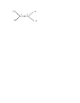
Figure 3: Diagrams of annihilation channels of $\nu_{\mbox{\tiny 2L,2R}}^{\mbox{\tiny KK}}$ to SM particles through $Z-Z^{\prime}$ mixing.

Due to $Z-Z^{\prime}$, there can also be annihilation of KK neutrino into SM Higgs, charged bosons, as well as fermion-antifermion pairs. The diagrams for these processes are shown in Fig. 3. In the limit that $v_{w}\ll v_{\mbox{\tiny R}}$, we can work to the leading-order in the expansion of $\mathcal{O}(v^{2}_{w}/v^{2}_{\mbox{\tiny R}})$, where we can estimate these processes by treating the $Z-Z^{\prime}$ mixing as a mass-insertion. In terms of Feynman diagrams, these annihilation channels are $s$-channel processes, where a pair KK neutrino annihilates into a $Z^{\prime}$-boson, which propagates to the mixing vertex, converting $Z^{\prime}$ to $Z$, which then decays into $h^{\ast}h$ (both neutral and charged), massless $W^{+}W^{-}$ or $\overline{f}{f}$. Compared to the amplitude of annihilation of KK neutrino into SM fermions without $Z-Z^{\prime}$ mixing, the annihilation through mixing have effectively a replaced propagator

$$\frac{1}{(s-M^{2}_{Z^{\prime}})}\rightarrow\frac{1}{(s-M^{2}_{Z^{\prime}})}\delta\!M^{2}\frac{1}{(s-M_{Z}^{2})}$$ (73)

where

$$\delta\!M^{2}\equiv\frac{g_{\mbox{\tiny{R}}}^{2}}{\sqrt{(g_{\mbox{\tiny{L}}}^{2}+g_{\mbox{\tiny{Y}}}^{2})(g_{\mbox{\tiny{R}}}^{2}+g_{\mbox{\tiny{BL}}}^{2})}}M_{Z}^{2},$$ (74)

is the off-diagonal element in the $Z-Z^{\prime}$ (mass)² matrix. Since $s\sim 4M^{2}_{\nu}=4R^{-2}$, the annihilation cross section into transverse gauge bosons and the Higgs bosons are suppressed by a factor of $M_{Z}^{4}/s^{2}\sim(100GeV)^{4}/16(500GeV)^{4}\sim 10^{-4}$, and can therefore be neglected. The same is true for the annihilation to fermion-antifermion pairs of the SM; we can ignore the effects of $Z-Z^{\prime}$ mixing in these channels. As for the longitudinal modes, the ratio of annihilation cross-sections of the longitudinal modes of the gauge bosons to the one single mode of SM fermion-antifermion pair is roughly

$$\frac{\sigma(\nu^{\mbox{\tiny KK}}\nu^{\mbox{\tiny KK}}\rightarrow W^{+}W^{-})}{\sigma(\nu^{\mbox{\tiny KK}}\nu^{\mbox{\tiny KK}}\rightarrow\overline{f}{f})}\sim\left(\frac{\delta M^{2}}{m_{W}^{2}}\right)^{2}.$$ (75)

This ratio is about $\tfrac{1}{2}$ for $g_{\mbox{\tiny{R}}}=0.7g_{\mbox{\tiny{L}}}$. As there is only one annihilation mode into the longitudinal modes of the charged gauge bosons, whereas there are many annihilation channels to the SM fermion-antifermion pairs, the total annihilation cross section is dominated by the SM fermion-antifermion contributions.

4.2 Co-annihilation Contributions to the Relic Density of $\nu_{\mbox{\tiny 2L,2R}}$

In the MUED model, the KK mode of the left-handed electron, $e_{\mbox{\scriptsize L}}^{\mbox{\tiny KK}}$, is expected to be nearly degenerate with the KK mode of the left-handed neutrino. The self- and co-annihilation contribution of $e_{\mbox{\scriptsize L}}^{\mbox{\tiny KK}}$ has been studied in the literature [1] [5], where it is shown that including such effects do not significantly alter the qualitative results, and that $\nu_{\mbox{\scriptsize L}}^{\mbox{\tiny KK}}$ with a slightly different mass can still account for the observed relic density. (However, $\nu_{\mbox{\scriptsize L}}^{\mbox{\tiny KK}}$ is ruled out by the direct detection experiments. This will be discussed in detail in Section 7.)

For our current model, the story is different. As can be seen in Eq. 42, $e_{\mbox{\tiny 2L,2R}}$, the partners of $\nu_{\mbox{\tiny 2L,2R}}$ under $SU(2)_{2}$, carry different quantum numbers under the $Z_{2}\times Z_{2}^{\prime}$ orbifold, and thus do not have $(10)$ nor $(01)$ modes. There are states that are nearly degenerate with $\nu_{\mbox{\tiny 2L,2R}}$, such as the $e^{\prime}$ states. However, these states interact with $\nu_{\mbox{\tiny 2L,2R}}$ only through Yukawa interactions, which can be ignored. Therefore, we expect effects of self- and co-annihilation with $\nu_{\mbox{\tiny 2L,2R}}$ nearby states to be even smaller than the MUED case, and ignore all such effects in our analysis.

4.3 Important Differences in Comparison to Standard Analysis

We note here that our our analysis of the annihilation channels for $\nu^{\mbox{\tiny KK}}_{\mbox{\tiny 2L,2R}}$ differ from those of [1] and [20] for $\nu^{\mbox{\tiny KK}}_{\mbox{\scriptsize L}}$ in two important ways. First, in their analysis, the $s$-channel process is mediated by $Z$-boson of the SM, whose mass can be ignored, whereas we have $s$-channel processes mediated by $Z^{\prime}$, whose mass is significantly larger than the mass of our dark matter candidate in the region of interest. Second, to a good approximation we can discard $t$,$u$-channel processes mediated by charged gauge bosons $W_{2}^{\pm}$, because $m^{2}_{W_{2}^{\pm}}$ has contributions both from $R^{-1}$ and $v_{\mbox{\tiny R}}$. To see this, let us make the approximation $m^{2}_{W^{\pm}}=m^{2}_{Z^{\prime}}+R^{-2}$, then we compare the cross section involving the product of a $t$ or $u$ diagram with a $s$-channel diagram $\sigma_{st}$ with that coming from the square of an $s$-channel diagram $\sigma_{ss}$,

$$\frac{\sigma_{ss}}{\sigma_{st}}\approx\frac{m^{2}_{\nu}+m^{2}_{W^{\pm}}}{4m^{2}_{\nu}-m^{2}_{Z^{\prime}}}=\frac{{2(R^{-1})^{2}+m^{2}_{Z^{\prime}}}}{4(R^{-1})^{2}-m^{2}_{Z^{\prime}}}.$$ (76)

Then $\sigma_{ss}\gg\sigma_{st}$ would require that

$$\frac{{2(R^{-1})^{2}+m^{2}_{Z^{\prime}}}}{4(R^{-1})^{2}-m^{2}_{Z^{\prime}}}\gg 1\quad\rightarrow\quad m^{2}_{Z^{\prime}}\gg 2(R^{-1})^{2},$$ (77)

which is satisfied in the region of interest in the parameter space. Similarly, the cross section involving two $t-$ or $u$-channel diagrams, $\sigma_{tt},\sigma_{uu}$ or $\sigma_{tu}$ is small compared to $\sigma_{ss}$.

5 Dark Matter Candidate II: $B^{\mbox{\tiny(11)}}_{\mbox{\tiny(-)}}$ or $B^{\mbox{\tiny(11)}}_{\mu}$

The lightest (11) mode is either $B^{\mbox{\tiny(11)}}_{\mbox{\tiny(-)}}$ or $B^{\mbox{\tiny(11)}}_{\mu}$, depending on radiative corrections. Although in Reference [24] found that $B^{\mbox{\tiny(11)}}_{\mu}$ is heavier than $B^{\mbox{\tiny(11)}}_{\mbox{\tiny(-)}}$, this result is specific the choice of orbifold in that particular case, and may not apply to $Z_{2}\times Z_{2}^{\prime}$ orbifold that we have here. Instead of performing the radiative corrections to determine which of the two particles is lighter, we will do a phenomenological study exploring both of these cases. To simplify the notation, we will often discard the $(11)$ superscript in the fields.

5.1 (Co)-Annihilation Channels of $B^{\mbox{\tiny(11)}}_{\mu}$

When $v_{w}\ll R^{-1}$, $B^{\mbox{\tiny(11)}}_{\mu}$ is same as $A^{\mbox{\tiny(11)}}_{Y,\mu}$, the KK mode of the photon up to small mixing effects. The annihilation channels and cross sections of $B^{\mbox{\tiny(11)}}_{\mu}$ have been studied in detail in [1] and [5], and in this subsection we summarize their results.

Figure 4: Annihilation channels of a pair of $B^{\mbox{\tiny(11)}}_{\mu}$ into SM fermion-antifermion pair.

$B^{\mbox{\tiny(11)}}_{\mu}$ can annihilate itself into a fermion-antifermion pair through $t$- and $u$-channel processes mediated by the (11) mode of the fermion (Fig. 4). It is important to note that the left- and right-handed fermions of SM have separate massive KK modes with vector-like couplings to the zero-mode fermion and $B^{\mbox{\tiny(11)}}_{\mu}$. The annihilation cross section can be written as

$$\sigma(B^{\mbox{\tiny(11)}}_{\mu}B^{\mbox{\tiny(11)}}_{\mu}\rightarrow\overline{f}f)=g_{1}^{4}(Y_{L}^{2}+Y_{\mbox{\tiny R}}^{4})N_{c}\frac{10(2M_{f}^{2}+s)\mbox{ArcTanh}(\beta)-7s\beta}{72\pi s^{2}\beta^{2}},$$ (78)

where $M_{f}=\sqrt{2}R^{-1}$ is the mass of the KK-fermion exchanged, $N_{c}$ is the color factor in the final state (3 for quarks and 1 for leptons), and $Y_{L,R}$ is the hypercharge of the left- and right-handed fermion. Summing over all SM fermions gives

$$\sum_{f\in\mbox{\tiny SM}}N_{c}(Y_{L}^{4}+Y_{\mbox{\tiny R}}^{4})=3(Y^{4}_{e_{L}}+Y^{4}_{e_{\mbox{\tiny R}}}+Y^{4}_{\nu_{L}}+3(Y^{4}_{u_{L}}+Y^{4}_{u_{\mbox{\tiny R}}}+Y^{4}_{d_{L}}+Y^{4}_{d_{\mbox{\tiny R}}}))=\frac{95}{18}.$$ (79)

There are also annihilation channels to Higgs through $t$- and $u$-channel processes mediated by a (11) mode of the Higgs boson as well as a quartic interaction. The annihilation cross section is given by

$$\sigma(B^{\mbox{\tiny(11)}}_{\mu}B^{\mbox{\tiny(11)}}_{\mu}\rightarrow h^{\ast}h)=\frac{g_{1}^{4}Y^{4}_{\phi}}{6\pi\beta s},$$ (80)

where $Y_{\phi}=1/2$ is the hypercharge of the Higgs doublet. By summing over two complex Higgs doublets, we have taken into account the annihilation into the longitudinal zero modes of the $W$ and $Z$ gauge bosons.

In the MUED, the KK mode with mass closest to $B^{\mbox{\tiny(1)}}_{\mu}$ is the KK mode of the right-handed electron $e^{(1)}_{\mbox{\tiny R}}$ when radiative corrections are included [22]. However, compared to the case without co-annihilation, the qualitative results of the relic density due to $B^{\mbox{\tiny(1)}}_{\mu}$ remains the same when one includes the co-annihilation $e^{(1)}_{\mbox{\tiny R}}B^{\mbox{\tiny(1)}}_{\mu}\rightarrow e_{R}A_{\mu}$ [1]. As pointed out by [1], this is because there are only two channel of such co-annihilation, leading to a small co-annihilation cross section, and thus small change in the relic density for a fixed $R^{-1}$.

In our case, we expect $B^{\mbox{\tiny(11)}}_{\mbox{\tiny(-)}}$ (which has no MUED analog) to be close in mass to $B^{\mbox{\tiny(11)}}_{\mu}$ in addition to $e^{(11)}_{1R}$ (the analog of $e^{(1)}_{\mbox{\tiny R}}$ in MUED). Furthermore, the co-annihilation $B^{\mbox{\tiny(11)}}_{\mu}B^{\mbox{\tiny(11)}}_{\mbox{\tiny(-)}}\rightarrow XX$ is significant as $B^{\mbox{\tiny(11)}}_{\mu}B^{\mbox{\tiny(11)}}_{\mbox{\tiny(-)}}$ can annihilate to all SM fermions through $t$- and $u$-channel processes mediated by a KK fermion. The co-annihilation cross section to fermion-antifermion pair is

$$\sum_{f\in\mbox{\tiny SM}}\sigma(B^{\mbox{\tiny(11)}}_{\mu}B^{\mbox{\tiny(11)}}_{\mbox{\tiny(-)}}\rightarrow\overline{f}f)=g_{1}^{4}\frac{95}{18}\frac{\mbox{ArcTan}(\beta)}{12\pi s\beta^{2}}.$$ (81)

Although the co-annihilation effect was overlooked in [4], the most important conclusions of our previous work remain the same, as we will show later.

5.2 (Co)-Annihilation Channels of $B^{\mbox{\tiny(11)}}_{\mbox{\tiny(-)}}$

The coupling of $B^{\mbox{\tiny(11)}}_{\mbox{\tiny(-)}}$ to matter fields in the full 6D-Lagrangian is given by (in four-component notation)

$$\mathcal{L}^{\mbox{\tiny 6D}} =\frac{g_{1}Y}{\sqrt{2}}B_{\mbox{\tiny Y,-}}\left[\overline{\Psi}_{-}(i\gamma_{5}-\mathbf{1})\Psi_{-}+\overline{\Psi}_{+}(i\gamma_{5}+\mathbf{1})\Psi_{+}\right]$$

$$=\frac{g_{1}Y}{\sqrt{2}}B_{Y,-}\left[(-i-1)\overline{\Psi}_{\mbox{\tiny-L}}\Psi_{\mbox{\tiny-R}}+(i-1)\overline{\Psi}_{\mbox{\tiny-R}}\Psi_{\mbox{\tiny-L}}+(-i+1)\overline{\Psi}_{\mbox{\tiny+L}}\Psi_{\mbox{\tiny+R}}+(i+1)\overline{\Psi}_{\mbox{\tiny+R}}\Psi_{\mbox{\tiny+L}}\right].$$ (82)

In terms of KK-modes, $B^{\mbox{\tiny(11)}}_{\mbox{\tiny(-)}}$ will couple to fermion fields in (00-fermion)(11-fermion) pairs, and its annihilation channels to fermions will proceed through $t-$ and $u-$processes mediated by a KK-fermion. The annihilation cross section is

$$\sum_{f\in\mbox{\scriptsize SM}}\sigma(B^{\mbox{\tiny(11)}}_{\mbox{\tiny(-)}}B^{\mbox{\tiny(11)}}_{\mbox{\tiny(-)}}\rightarrow\overline{f}f)=g_{1}^{4}\frac{95}{18}\frac{2(2M_{f}^{2}+s)\mbox{ArcTan}(\beta)-3s\beta}{2\pi s\beta^{2}}.$$ (83)

In the non-relativistic limit, this cross-section is $p$-wave suppressed. There is also annihilation to a pair of Higgs bosons through the quartic coupling

$$\mathcal{L}^{\mbox{\tiny 4D}} =g_{1}^{2}Y_{H}^{2}B^{\mbox{\tiny(11)}}_{\mbox{\tiny(-)}}B^{\mbox{\tiny(11)}}_{\mbox{\tiny(-)}}H^{{\dagger}\mbox{\tiny(00)}}H^{\mbox{\tiny(00)}},$$ (84)

and this gives a cross section of

$$\langle\sigma v_{\mbox{\tiny rel}}\rangle=\frac{g_{1}^{4}Y_{H}^{4}}{2\pi s}.$$ (85)

Because the annihilation of $B^{\mbox{\tiny(11)}}_{\mbox{\tiny(-)}}$ to fermion modes is $p$-wave suppressed, the relic density resulting $B^{\mbox{\tiny(11)}}_{\mbox{\tiny(-)}}$ self-annihilation channels would in general be too high. Therefore, we must rely on co-annihilation channels such as $B^{\mbox{\tiny(11)}}_{\mu}B^{\mbox{\tiny(11)}}_{\mbox{\tiny(-)}}\rightarrow XX$ to obtain observed relic density, as we will see in the next section.

6 Numerical Results of Relic Density

The main free parameters of our theory are $R^{-1}$ and $M_{Z^{\prime}}$, and the mass-splitting $\Delta\equiv(M_{B^{\mbox{\tiny(11)}}_{\mu}}-M_{B^{\mbox{\tiny(11)}}_{\mbox{\tiny(-)}}})/M_{B^{\mbox{\tiny(11)}}_{\mbox{\tiny(-)}}}$. In addition, we have $g_{\mbox{\tiny{R}}}$ or $g_{\mbox{\tiny{BL}}}$ as a free parameter as long as we can satisfy the constraint

$$g_{1}^{2}=\frac{g_{\mbox{\tiny{BL}}}^{2}g_{\mbox{\tiny{R}}}^{2}}{g_{\mbox{\tiny{BL}}}^{2}+g_{\mbox{\tiny{R}}}^{2}}.$$

6.1 $B^{\mbox{\tiny(11)}}_{\mu}$-$\nu^{\mbox{\tiny(01)}}_{\mbox{\tiny 2L,2R}}$ Dark Matter

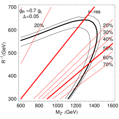
Figure 5: The plot on the left shows the contour in the $R^{-1}-M_{Z^{\prime}}$ plane that corresponds to $\Omega_{\nu_{L,R}}h^{2}+\Omega_{B_{Y}}h^{2}$ being the observed dark matter. The intersection of the red lines with the contour indicate the the fraction of KK neutrinos in the dark matter. The plot on the right shows $\Omega_{B_{Y}}h^{2}$ as a function of $\Delta$ for various values of $R^{-1}$.

For $\Delta=0.05$, we present the allowed region in $R^{-1}-M_{Z^{\prime}}$ space that gives the observed dark matter relic density in the first plot of Fig. 5. Since both $B^{\mbox{\tiny(11)}}_{\mu}$ and $\nu^{\mbox{\tiny(01)}}_{\mbox{\tiny 2L,2R}}$ can independently give the correct relic density without co-annihilation from other modes with almost degenerate mass, varying $\Delta$ does not affect the qualitative results of what we present below. The independence of $\Omega_{B^{\mbox{\tiny(11)}}_{\mu}}h^{2}$ on $\Delta$ as can be seen in the second plot of Fig. 5. For small values of $M_{Z^{\prime}}$, the annihilation of $\nu^{\mbox{\tiny(01)}}_{\mbox{\tiny 2L,2R}}$ is efficient and most of the dark matter is $B^{\mbox{\tiny(11)}}_{\mu}$ having a mass of roughly $\sqrt{2}R^{-1}\sim 700$ GeV. In fact, along the line $2M_{\nu^{(01)}}=2R^{-1}=M_{Z^{\prime}}$, the annihilation of $\nu^{\mbox{\tiny(01)}}_{\mbox{\tiny 2L,2R}}$ has an $s$-channel resonance, and its contribution to dark matter relic density is minimal. Away from the line of $s$-channel resonance, the contribution of $\nu^{\mbox{\tiny(01)}}_{\mbox{\tiny 2L,2R}}$ to the relic density increases, and $R^{-1}$ decreases so as to decrease the relic density due to $B^{\mbox{\tiny(11)}}_{\mu}$, keeping the total relic density within the allowed range.

The current experimental bound on the massive, neutral, vector boson is $M_{Z^{\prime}}>800$ GeV. If we further impose the bound that $R^{-1}>400$ GeV, the allowed region in the parameter space is very limited.

6.2 $B^{\mbox{\tiny(11)}}_{\mbox{\tiny(-)}}$-$\nu^{\mbox{\tiny(01)}}_{\mbox{\tiny 2L,2R}}$ Dark Matter

Figure 6: The plot on the left shows the allowed region in the parameter space that gives rise to the observed dark matter relic density for $g_{\mbox{\tiny{R}}}=0.7g_{\mbox{\tiny{L}}}$ and different values of $\Delta$. On the right, we plot the relic density due to $B^{\mbox{\tiny(11)}}_{\mbox{\tiny(-)}}$ as a function of the mass-splitting $\Delta$ for various values of $R^{-1}$.

As stated earlier, $B^{\mbox{\tiny(11)}}_{\mbox{\tiny(-)}}$ by itself can not annihilate efficiently enough to account for the observed relic abundance. However, there is significant co-annihilation process $B^{\mbox{\tiny(11)}}_{\mbox{\tiny(-)}}B^{\mbox{\tiny(11)}}_{\mu}\rightarrow\overline{f}f$. In Fig. 6, we show contours that give the observed relic density for various values of $\Delta$. We see that when $B^{\mbox{\tiny(11)}}_{\mbox{\tiny(-)}}$ and $B^{\mbox{\tiny(11)}}_{\mu}$ are nearly degenerate to less than 5%, then the distribution of dark matter among $\nu^{\mbox{\tiny(01)}}_{\mbox{\tiny 2L,2R}}$ and $B^{\mbox{\tiny(11)}}_{\mbox{\tiny(-)}}$ is similar to the previous case. When the mass splitting between $B^{\mbox{\tiny(11)}}_{\mbox{\tiny(-)}}$ and $B^{\mbox{\tiny(11)}}_{\mu}$ is larger than 5%, however, the model is ruled out as we can not obtain the observed relic density without violating $R>400$ GeV bound. When $B^{\mbox{\tiny(11)}}_{\mbox{\tiny(-)}}$ and $B^{\mbox{\tiny(11)}}_{\mu}$ are nearly degenerate, $\nu^{\mbox{\tiny(KK)}}_{\mbox{\tiny 2L,2R}}$ can still contribute significantly to the observed relic density when $M_{Z^{\prime}}$ is about $1.2$ TeV and $R^{-1}\sim 400$ GeV.

7 Direct Detection of Two-Component Dark Matter

As we have a two-component dark matter, the total dark matter-nucleon cross section is given by

$$\sigma_{n}=\kappa_{\nu_{\mbox{\tiny R}}}\sigma_{\nu_{\mbox{\tiny R}}}+\kappa_{B}\sigma_{B},$$ (86)

where $\sigma_{\nu_{\mbox{\tiny R}}(B)}$ is the spin-independent KK neutrino (hypercharge vector or pseudoscalar)- nucleon scattering cross section, and

$$\kappa_{\nu_{\mbox{\tiny R}}}\equiv\frac{\Omega_{\nu_{\mbox{\tiny R}}}h^{2}}{\Omega_{\nu_{\mbox{\tiny R}}}h^{2}+\Omega_{B}h^{2}},$$ (87)

is the fractional contribution of the KK neutrino relic density to the total relic density of the dark matter. $\kappa_{B}$ is similarly defined. As pointed out in Ref. [1], $\sigma_{B}$ is of the order $\sigma_{B}\sim 10^{-10}$ pb, and we will find that $\sigma_{\nu_{\mbox{\tiny R}}}\gg\sigma_{B}$. Therefore, it is a good approximation to take $\sigma_{n}$ as

$$\sigma_{n}\approx\kappa_{\nu_{\mbox{\tiny R}}}\sigma_{\nu_{\mbox{\tiny R}}}.$$ (88)

The elastic cross section between $\nu_{\mbox{\tiny 2L,2R}}$ and a nucleon inside a nucleus $N(A,Z)$ is given by

$$\sigma_{0} =\frac{b_{N}^{2}m^{2}_{n}}{\pi A^{2}},$$ (89)

where $b_{N}=Zb_{p}+(A-Z)b_{n}$ and $b_{p,n}$ is the effective four-fermion coupling between $\nu_{\mbox{\tiny 2L,2R}}$ and nucleon. They are given by $b_{p}=2b_{u}+b_{d}$ and $b_{n}=b_{u}+2b_{d}$. In our case, although $\nu_{\mbox{\tiny 2L,2R}}$ only couples to $Z^{\prime}_{\mu}$ at leading order, we have to taken into account the $Z-Z^{\prime}$ mixing. We can including the effects of mixing up to order of $\mathcal{O}(M^{2}_{Z}/M^{2}_{Z^{\prime}})$ by treating the mixing as perturbations and include one vertex mixing. In this case, we have

$$b_{q} =\frac{1}{2M^{2}_{Z^{\prime}}}g_{(\overline{\nu_{2}}{\nu_{2}}Z^{\prime})}\left[(g_{(\overline{q}_{L}{q}_{L}Z^{\prime})}+g_{(\overline{q}_{\mbox{\tiny R}}{q}_{\mbox{\tiny R}}Z^{\prime})})-(g_{(\overline{q}_{L}{q}_{L}Z)}+g_{(\overline{q}_{\mbox{\tiny R}}{q}_{\mbox{\tiny R}}Z)})\frac{\delta\!M^{2}}{M^{2}_{Z}}+\mathcal{O}\left(\frac{M^{2}_{Z}}{M^{2}_{Z^{\prime}}}\right)\right],$$ (90)

where

$$\delta\!M^{2}\equiv\frac{g_{\mbox{\tiny{R}}}^{2}}{\sqrt{(g_{\mbox{\tiny{L}}}^{2}+g_{\mbox{\tiny{Y}}}^{2})(g_{\mbox{\tiny{R}}}^{2}+g_{\mbox{\tiny{BL}}}^{2})}}M_{Z}^{2}$$ (91)

is the mixing between $Z$ and $Z^{\prime}$ (see Eq. 59).

The prospects of direct detection of $B^{\mbox{\tiny(11)}}_{\mu}$ has been studied extensively, and the calculated detection rates are beyond the reach of current experiments. As for $B^{\mbox{\tiny(11)}}_{\mbox{\tiny(-)}}$, because there is no $s$-wave for elastic scattering $B^{\mbox{\tiny(11)}}_{\mbox{\tiny(-)}}N\rightarrow B^{\mbox{\tiny(11)}}_{\mbox{\tiny(-)}}N$, the cross-section is suppressed by a factor of $v_{\mbox{\tiny rel}}^{2}\sim 10^{-5}$. Therefore, we expect that the direct detection rates of $\nu^{(10)}_{\mbox{\tiny 2L,2R}}$ will dominate that of both $B^{\mbox{\tiny(11)}}_{\mu}$ and $B^{\mbox{\tiny(11)}}_{\mbox{\tiny(-)}}$. This is one of the main points of our work: the lightest KK-mode of sterile neutrino as dark matter candidate could be detected directly in the current and the next rounds of direct-detection experiments if its relic density is significant compared to the observed total relic density, in contrast to other dark matter candidates in the literature, such as the neutralino of MSSM or the lightest KK-mode of the photon.

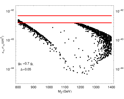
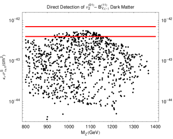
Figure 7: The plot on the left (right) shows the dark matter-nucleon cross-section as a function of $M_{Z^{\prime}}$ for the case where $B^{\mbox{\tiny(11)}}_{\mu}$ ($B^{\mbox{\tiny(11)}}_{\mbox{\tiny(-)}}$) is lightest (11) mode. The plots scan over different values of $R^{-1}$ and $-0.05<\Delta<0$ that gives the observed relic density. The horizontal lines correspond to the upper bounds on $\sigma_{n}$ from CDMS II for dark matter candidates with masses 300 and 500 GeV

In Fig. 7, we show the direct detection cross section as a function of $M_{Z^{\prime}}$ for both cases where $B^{\mbox{\tiny(11)}}_{\mu}$ and $B^{\mbox{\tiny(11)}}_{\mbox{\tiny(-)}}$ is the lighter of the two. The horizontal lines correspond to the upper bounds on $\sigma_{n}$ from CDMS II for dark matter candidates with masses 300 and 500 GeV, which are about 4$\times 10^{-43}\mbox{cm}^{2}$ and 7$\times 10^{-43}\mbox{cm}^{2}$, respectively.

A particularly interesting region in the parameter space is $R\sim 400$ GeV and $M_{Z^{\prime}}\sim 1200$ GeV. Here, the KK-sterile neutrino contributes to roughly half of the relic density. This admixture of dark matter is just below the current experimental bound from direct detection, as shown in Fig. 5, when we use the CDMS II bound that dark matter-nucleon spin-independent cross-section must not exceed $4\times 10^{-43}\mbox{cm}^{2}$ for a 400 GeV dark matter.

8 Some Phenomenological Implications

In this section, we give a qualitative comparision of the phenomenological implications of this model with those of the conventional left-right symmetric models [26]. It has long been recognized that two important characteristic predictions of the left-right models are the presence of TeV scale $W_{R}$ and $Z^{\prime}$ gauge bosons which can be detectable in high energy colliders [28]. In addition to the collider signatures of generic UED models [27], two predictions characteristic of the model discussed here which differ from those of the earlier models are : (i) The mass of $Z^{\prime}$ has an upper bound of about $1.5$ TeV and a more spectacular one where (ii) the $W_{R}$ in this model, being a KK excitation, does not couple to a pair of the known standard model fermions which are zero modes. This property of the $W_{R}$ has a major phenomenological impact and will require a completely new analysis of constraints on this e.g. the well known $K_{L}-K_{S}$ mass difference constraint on $M_{W_{R}}$ [29] does not apply here since the mixed $W_{L}-W_{R}$ exchange box graph responsible for the new contribution to $K_{L}-K_{S}$ mass difference does not exist. The box graph where both exchange particles are $W_{R}$’s exists but its contribution to the $\Delta S=2$ Hamiltonian is suppressed compared to the left-handed one by a factor $\left(\frac{M_{W_{L}}}{M_{W_{R}}}\right)^{4}$ and gives only a very weak bound on $M_{W_{R}}$.

Also, the bounds from muon and beta decay [30] are nonexistent for the same reason because there is no tree level $W_{R}$ contribution to these processes. Furthermore, in this model, there is no $W_{L}-W_{R}$ mixing unlike the conventional left-right models.

Because of this property, the decay modes and production mechanism of the $W_{R}$ are also very different from the case of the conventional left-right model, while the decay modes and production mechanism of the $Z^{\prime}$ remain the same. We do not discuss the $Z^{\prime}$ case which has been very widely discussed in literature.

The $W_{R}$ will have a mass given by As far as the $W_{R}$ is concerned, it is given by the formula $M^{2}_{W_{R}}\sim\frac{cos^{2}\theta_{W}}{cos2\theta_{W}}M^{2}_{Z^{\prime}}$. Furthermore, it can only be pair produced and will decay to $u^{\prime}_{\mbox{\tiny 2L}}\bar{d^{\prime}}_{\mbox{\tiny 2L}},\ u_{\mbox{\tiny 2R}}\bar{d}_{\mbox{\tiny 2R}},\ u^{\prime}_{\mbox{\tiny 2R}}\bar{d^{\prime}}_{\mbox{\tiny 2R}},\ u_{\mbox{\tiny 2L}}\bar{d}_{\mbox{\tiny 2L}},\ \bar{e}_{\mbox{\tiny 2L,R}}\nu_{\mbox{\tiny 2L,R}},$ and $\bar{e^{\prime}}_{\mbox{\tiny 2L,R}}\nu^{\prime}_{\mbox{\tiny 2L,R}}$. For sub-TeV $W_{R}$, only the decay modes $\bar{e^{\prime}}_{\mbox{\tiny 2L}}\nu^{\prime}_{\mbox{\tiny 2L}}$ and $u_{\mbox{\tiny 2R}}\bar{d}_{\mbox{\tiny 2R}}$ will dominate depending on the precise value of $W_{R}$ mass and the $R^{-1}$. The leptonic decay mode will look very similar to the supersymmetric case where pair-produced sleptons will decay to a lepton and the neutralino. The hadronic channel will however look different from the squark case. The further details of the collider signature of our model is currently under investigation and will be presented separately.

9 Conclusions

In summary, we have studied the profile of cold dark matter candidates in a Universal Extra Dimension model with a low-scale extra $W_{\mbox{\tiny R}}$ and $Z^{\prime}$. There are two possible candidates: $\nu^{\mbox{\tiny KK}}_{\mbox{\tiny R}}$ and either the $B^{\mbox{\tiny(11)}}_{\mbox{\tiny(-)}}$ or $B^{\mbox{\tiny(11)}}_{\mu}$ depending on which one receives less radiative corrections. We have done detailed calculation of the relic density of these particles as a function of the parameters of the model which are $g_{\mbox{\tiny R}}$, $R^{-1}$ and $M_{Z^{\prime}}$. We find upper limits on these parameters where the above KK modes can be cold dark matter of the universe. In discussing the relic abundance, we have considered the co-annihilation effect of nearby states. We also calculate the direct detection cross-section in current underground detectors for the entire allowed parameter range in the model and we find that, for the case where KK neutrino contributes significantly to the total relic density, the lowest possible value of the cross-section predicted by our model is accessible to the current and/or planned direct search experiments. Therefore, the most interesting region of our model can not only be tested in the colliders but also these dark matter experiments. Combined with LHC search for the $Z^{\prime}$ of left-right model, dark matter experiments could rule out this model.

10 Acknowledgement

The work of K.H and R.N.M is supported by the National Science Foundation grant no. Phy-0354401. S.N is supported by the DOE grant no. Phy. DE-FG02-97ER41029.

Appendix A Fields on $T^{2}/{Z_{2}\times Z^{\prime}_{2}}$

For convenience of type-setting, we define the functions

$$c(i,j)\equiv\cos\frac{ix^{5}+jx^{6}}{R},\quad\quad s(i,j)\equiv\sin\frac{ix^{5}+jx^{6}}{R},$$

$$c^{\prime}(i,j)\equiv\cos\frac{ix^{\prime 5}+jx^{\prime 6}}{R},\quad\quad s^{\prime}(i,j)\equiv\sin\frac{ix^{\prime 5}+jx^{\prime 6}}{R},$$ (92)

And for reference we will make use of this integral

$$\int_{0}^{2\pi R}\!\!\!\!\!\!\!\!dx^{5}\int_{0}^{2\pi R}\!\!\!\!\!\!\!\!dx^{6}c(i,j)c(m,n)=\int_{0}^{2\pi R}\!\!\!\!\!\!\!\!dx^{5}\int_{0}^{2\pi R}\!\!\!\!\!\!\!\!dx^{6}s(i,j)s(m,n)=2\pi^{2}R^{2}\delta_{im}\delta{jn}$$ (93)

for positive integers $i,j,m$ and $n$, extensively. We have the compactified space $2\pi R\times 2\pi R$ by imposing the periodic boundary conditions on the fields

$$\phi(x^{\mu},x^{4},x^{5})=\phi(x^{\mu},x^{4}+2\pi R,x^{5})=\phi(x^{\mu},x^{4},x^{5}+2\pi R).$$ (94)

The periodic boundary conditions mean that we can write the fields in the form of

$$\phi(x^{\mu},x^{4},x^{5})=\sum_{n,m}\left(c(n,m)\varphi^{(nm)}(x^{\mu})+s(n,m)\tilde{\varphi}^{(nm)}(x^{\mu})\right).$$ (95)

On top of the periodic boundary conditions, we impose two orbifolding symmetries on our theory

$$Z_{2}:{\bf{y}}\rightarrow-{\bf{y}},\quad Z_{2}^{\prime}:{\bf{y^{\prime}}}\rightarrow-{\bf{y^{\prime}}}.$$ (96)

with ${\bf y^{\prime}}={\bf y}-(\pi R/2,\pi R/2)$. Demanding that the Lagrangian be invariant under the orbifolding symmetries, we can assign parities to the fields under the discrete transformations and remove roughly half of the KK modes in Eq. 95. The choices of signs are motivated by the desired phenomenology. In our case, we have two orbifolding symmetries, so we can assign two signs to a given field. There are four possibilities: $(+,\pm)$ and $(-,\pm)$, and we examine each case separately.

For $(+,\pm)$ case, we have the general expansion

$$\phi^{(+,\pm)}(x^{\mu},x^{4},x^{5}) =\frac{1}{2\pi R}\sum_{n,m=0}^{\infty}\left(c(n,m)\varphi^{(nm)}\right)$$

$$=\frac{1}{2\pi R}\sum_{n,m=0}^{\infty}\left[\left(c^{\prime}(n,m)\cos\frac{(m+n)\pi}{2}-s^{\prime}(n,m)\sin\frac{(m+n)\pi}{2}\right)\varphi^{(nm)}\right].$$ (97)

So we see that for $(+,+)$ fields, we need $n+m$ and $n-m$ to be even.

For $(+,-)$ fields, we need $n+m$ and $n-m$ to be odd. For $(-,\pm)$ case, we have the general expansion

$$\phi^{(-,\pm)}(x^{\mu},x^{4},x^{5}) =\frac{1}{2\pi R}\sum_{n+m\geq 1}^{\infty}\left(s(n,m)\varphi^{(nm)}\right)$$

$$=\frac{1}{2\pi R}\sum_{n+m\geq 1}^{\infty}\left[\left(s^{\prime}(n,m)\cos\frac{(m+n)\pi}{2}+c^{\prime}(n,m)\sin\frac{(m+n)\pi}{2}\right)\varphi^{(nm)}\right].$$ (98)

So we see that for $(-,+)$ fields, we need $n+m$ and $n-m$ to be odd. For $(-,-)$ fields, we need $n+m$ and $n-m$ to be even. Of course, for the $(-,\pm)$ cases, we can not have $(m,n)=(0,0)$ mode.

Appendix B Normalization of Fields and Couplings

B.1 Matter Fields

The dark matter candidates of the theory are the first KK modes of the neutrinos charged under $SU(2)_{2}$. They have the $Z_{2}\times Z_{2}^{\prime}$ charges: $\nu_{\mbox{\tiny 2L}}(-,+),\nu_{\mbox{\tiny 2R}}(+,-)$. If we let $\overrightarrow{n}=(n,m)$, we see each of $\nu_{\mbox{\tiny 2L,2R}}$ has two independent modes: $\overrightarrow{n}=(1,0)$ and $\overrightarrow{n}=(0,1)$. These are two independent Dirac particles in the sense that there is no mixing at tree level in the effective 4D theory.

We expand the kinetic energy term

$$\mathcal{L}_{\mbox{\tiny 6D-KE}} =i\overline{\Psi}\Gamma^{M}\partial_{M}\Psi$$

$$=i\begin{pmatrix}\overline{\Psi}_{-}&\overline{\Psi}_{+}\end{pmatrix}\begin{pmatrix}0&\gamma^{\mu}\partial_{\mu}+i\gamma_{5}\partial_{5}+\partial_{6}\\ \gamma^{\mu}\partial_{\mu}+i\gamma_{5}\partial_{5}-\partial_{6}&0\end{pmatrix}\begin{pmatrix}\Psi_{+}\\ \Psi_{-}\end{pmatrix}$$

$$=i\overline{\Psi}_{-}(\gamma^{\mu}\partial_{\mu}+i\gamma_{5}\partial_{5}+\partial_{6})\Psi_{-}+i\overline{\Psi}_{+}(\gamma^{\mu}\partial_{\mu}+i\gamma_{5}\partial_{5}-\partial_{6})\Psi_{+}.$$ (99)

Note that $\Psi$ is an eight-component object, while $\Psi_{\pm}$ are four-component, six-dimensional chiral spinors. We denote six-dimensional chirality by $\pm$ and four-dimensional chirality by $L,R$. Each six-dimensional chiral spinor is vector-like in the four-dimensional sense, and each is a Dirac spinor. Since our dark matter candidate is of (-1) 6D-chirality, we only deal with the first part of the kinetic energy term, and drop the subscript.

Since we are after the coefficients, we expand in detail the first KK mode of the dark matter candidate.

$$\mathcal{L}_{\mbox{\tiny 6D-KE}} \supset i\overline{\Psi}_{-}(\gamma^{\mu}\partial_{\mu}+i\gamma_{5}\partial_{5}+\partial_{6})\Psi_{-}$$

$$=i\begin{pmatrix}\Psi^{{\dagger}}_{L}&\Psi^{{\dagger}}_{\mbox{\tiny R}}\end{pmatrix}\begin{pmatrix}i\partial_{5}+\partial_{6}&\sigma^{\mu}\partial_{\mu}\\ \overline{\sigma}^{\mu}\partial_{\mu}&-i\partial_{5}+\partial_{6}\end{pmatrix}\begin{pmatrix}\Psi_{\mbox{\tiny R}}\\ \Psi_{L}\end{pmatrix}$$

$$=i(\Psi^{{\dagger}}_{L}\sigma^{\mu}\partial_{\mu}\Psi_{L}+\Psi^{{\dagger}}_{\mbox{\tiny R}}\overline{\sigma}^{\mu}\partial_{\mu}\Psi_{\mbox{\tiny R}}+\Psi^{{\dagger}}_{L}(i\partial_{5}+\partial_{6})\Psi_{\mbox{\tiny R}}+\Psi_{\mbox{\tiny R}}(-i\partial_{5}+\partial_{6})\Psi_{L})$$ (100)

At this point, we use the KK-expansions. Noting the charge assignments $\nu_{2L}(-,+),\nu_{2R}(+,-)$, we expand the fields as

$$\nu_{\mbox{\tiny 2R}}=\frac{1}{\sqrt{2}\pi R}\left(c(1,0)\nu^{\mbox{\tiny(10)}}_{\mbox{\tiny 2R}}(x^{\mu})+c(0,1)\nu^{\mbox{\tiny(01)}}_{\mbox{\tiny 2R}}(x^{\mu})\right),$$

$$\nu_{\mbox{\tiny 2L}}=\frac{1}{\sqrt{2}\pi R}\left(s(1,0)\nu^{{\mbox{\tiny(10)}}}_{\mbox{\tiny 2L}}(x^{\mu})+is(0,1)\nu^{\mbox{\tiny(01)}}_{\mbox{\tiny 2L}}(x^{\mu})\right).$$ (101)

The four-dimensional effective Lagrangian is obtained by inserting the expansion of Eq. 101 into Eq. 100, and integrate $x^{5}$ and $x^{6}$ from $0$ to $2\pi R$. Following this procedure, we obtain

$$\mathcal{L}_{\mbox{\tiny 4D-eff}}=\int_{0}^{2\pi R}\!\!\!\!\!\!\!\!dx^{5}\int_{0}^{2\pi R}\!\!\!\!\!\!\!\!dx^{6}\mathcal{L}_{\mbox{\tiny 6D-KE}} =i\left(\nu_{\mbox{\tiny 2L}}^{{\dagger}\mbox{\tiny(10)}}\sigma^{\mu}\partial_{\mu}\nu_{\mbox{\tiny 2L}}^{\mbox{\tiny(10)}}+\nu_{\mbox{\tiny 2L}}^{{\dagger}\mbox{\tiny(01)}}\sigma^{\mu}\partial_{\mu}\nu_{\mbox{\tiny 2L}}^{\mbox{\tiny(01)}}+\nu_{\mbox{\tiny 2R}}^{{\dagger}\mbox{\tiny(10)}}\overline{\sigma}^{\mu}\partial_{\mu}\nu_{\mbox{\tiny 2R}}^{\mbox{\tiny(10)}}+\nu_{\mbox{\tiny 2R}}^{{\dagger}\mbox{\tiny(01)}}\overline{\sigma}^{\mu}\partial_{\mu}\nu_{\mbox{\tiny 2R}}^{\mbox{\tiny(01)}}\right)$$

$$\ \ -\frac{1}{R}\left((\nu_{\mbox{\tiny 2L}}^{{\dagger}\mbox{\tiny(10)}}\nu_{\mbox{\tiny 2R}}^{\mbox{\tiny(10)}}-\nu_{\mbox{\tiny 2R}}^{{\dagger}\mbox{\tiny(10)}}\nu_{\mbox{\tiny 2L}}^{\mbox{\tiny(10)}})-(\nu_{\mbox{\tiny 2L}}^{{\dagger}\mbox{\tiny(01)}}\nu_{\mbox{\tiny 2R}}^{\mbox{\tiny(01)}}-\nu_{\mbox{\tiny 2R}}^{{\dagger}\mbox{\tiny(01)}}\nu_{\mbox{\tiny 2L}}^{\mbox{\tiny(01)}})\right).$$ (102)

¿From this calculation, we see that we have two independent Dirac neutrinos that do not mix with each other: $\nu^{\mbox{\tiny(01)}}$ and $\nu^{\mbox{\tiny(10)}}$.

Following the same procedure, we can find the normalization of scalars.

$$\Phi(+,+) =\frac{1}{2\pi R}\phi^{(00)}+\frac{1}{\sqrt{2}\pi R}\sum_{m,n}\cos\frac{mx^{5}+nx^{6}}{R}\phi^{(mn)},$$

$$\Phi(+,-) =\frac{1}{\sqrt{2}\pi R}\sum_{m,n}\cos\frac{mx^{5}+nx^{6}}{R}\phi^{(mn)},$$

$$\Phi(-,+) =\frac{1}{\sqrt{2}\pi R}\sum_{m,n}\sin\frac{mx^{5}+nx^{6}}{R}\phi^{(mn)},$$

$$\Phi(-,-) =\frac{1}{\sqrt{2}\pi R}\sum_{m,n}\cos\frac{mx^{5}+nx^{6}}{R}\phi^{(mn)}.$$ (103)

Again, the rules of $m,n$ in the previous section for fermions apply to the scalars.

B.2 Gauge Bosons

As we are only interested in the normalization of the gauge fields, we consider a generic gauge boson, $\mathcal{A}_{M}$, associated with an $U(1)$ symmetry. We then have the expansion

$$\mathcal{L}_{gauge} =-\frac{1}{4}F^{MN}F_{MN}$$

$$=-\frac{1}{4}F_{\mu\nu}F^{\mu\nu}-\frac{1}{2}F_{5\mu}F^{5\mu}-\frac{1}{2}F_{6\mu}F^{6\mu}-\frac{1}{2}F_{56}F^{56}$$

$$=-\frac{1}{4}F_{\mu\nu}F^{\mu\nu}$$

$$\quad+\frac{1}{2}(\partial_{\mu}\mathcal{A}_{5}\partial^{\mu}\mathcal{A}_{5}+\partial_{5}\mathcal{A}_{\mu}\partial_{5}\mathcal{A}^{\mu}-\partial_{5}\mathcal{A}_{\mu}\partial^{\mu}\mathcal{A}_{5}-\partial_{\mu}\mathcal{A}_{5}\partial_{5}\mathcal{A}^{\mu})$$

$$\quad+\frac{1}{2}(\partial_{\mu}\mathcal{A}_{6}\partial^{\mu}\mathcal{A}_{6}+\partial_{6}\mathcal{A}_{\mu}\partial_{6}\mathcal{A}^{\mu}-\partial_{6}\mathcal{A}_{\mu}\partial^{\mu}\mathcal{A}_{6}-\partial_{\mu}\mathcal{A}_{6}\partial_{6}\mathcal{A}^{\mu})$$

$$\quad-\frac{1}{2}(\partial_{5}\mathcal{A}_{6}\partial_{5}\mathcal{A}_{6}+\partial_{6}\mathcal{A}_{5}\partial_{6}\mathcal{A}_{5}-2\partial_{5}\mathcal{A}_{6}\partial_{6}\mathcal{A}_{5})$$ (104)

Notice that we have made the changes $\mathcal{A}^{5,6}=-\mathcal{A}_{5,6},\partial^{5,6}=-\partial_{5,6}$, so that $\mathcal{A}_{5,6}$ should be treated as real, scalar fields. We will work with this equation for the various gauge particles.

As with the case of the neutral gauge bosons in our theory, we assign the $Z_{2}\times Z_{2}^{\prime}$ parities to be $\mathcal{A}_{\mu}(++)$ and $\mathcal{A}_{5,6}(--)$, and obtain the following lowest KK modes:

$$A^{\mbox{\tiny(00)}}_{\mu},\ A^{\mbox{\tiny(11)}}_{\mu},\ A^{\mbox{\tiny(20)}}_{\mu},\ A^{\mbox{\tiny(02)}}_{\mu},$$

$$A^{\mbox{\tiny(11)}}_{5},\ A^{\mbox{\tiny(20)}}_{5},\ A^{\mbox{\tiny(02)}}_{5},$$

$$A^{\mbox{\tiny(11)}}_{6},\ A^{\mbox{\tiny(20)}}_{6},\ A^{\mbox{\tiny(02)}}_{6},$$ (105)

and the KK-mode expansions for these states

$$\mathcal{A}_{\mu} =\frac{1}{2\pi R}A^{\mbox{\tiny(00)}}_{\mu}+\frac{1}{\sqrt{2}\pi R}\left(\cos\frac{2x^{5}}{R}A^{\mbox{\tiny(20)}}_{\mu}+\cos\frac{2x^{6}}{R}A^{\mbox{\tiny(02)}}_{\mu}+\cos\frac{x^{5}+x^{6}}{R}A^{\mbox{\tiny(11)}}_{\mu}\right),$$

$$\mathcal{A}_{5,6} =\frac{1}{\sqrt{2}\pi R}\left(\sin\frac{2x^{5}}{R}A^{\mbox{\tiny(20)}}_{5,6}+\sin\frac{2x^{6}}{R}A^{\mbox{\tiny(02)}}_{5,6}+\sin\frac{x^{5}+x^{6}}{R}A^{\mbox{\tiny(11)}}_{5,6}\right).$$ (106)

One may check that the normalization gives canonical fields for the scalars $A^{\mbox{\tiny KK}}_{5,6}$.

For the four-dimensional Lagrangian we insert the expansion of Eq. 106 into Eq. 104 and integrate over $x^{5}$ and $x^{6}$. In additional to canonical kinetic energy terms, we obtain the masses of these modes.

$$\mathcal{L} =\frac{1}{2}\left[\frac{4}{R^{2}}A_{\mu}^{\mbox{\tiny(20)}}A^{\mu,\mbox{\tiny(20)}}+\frac{4}{R^{2}}A_{\mu}^{\mbox{\tiny(02)}}A^{\mu,\mbox{\tiny(02)}}+\frac{2}{R^{2}}A_{\mu}^{\mbox{\tiny(11)}}A^{\mu,\mbox{\tiny(11)}}\right]$$

$$\!\!-\frac{1}{2}\left[\frac{4}{R^{2}}(A^{\mbox{\tiny(20)}}_{5})^{2}+\frac{4}{R^{2}}(A^{\mbox{\tiny(02)}}_{6})^{2}+\frac{1}{R^{2}}(A^{\mbox{\tiny(11)}}_{5})^{2}+\frac{1}{R^{2}}(A^{\mbox{\tiny(11)}}_{6})^{2}-2\frac{1}{R^{2}}A^{\mbox{\tiny(11)}}_{5}A^{\mbox{\tiny(11)}}_{6}\right]$$ (107)

We note first that we have some massless modes in $A_{6}^{\mbox{\tiny(02)}}$ and $A_{5}^{\mbox{\tiny(20)}}$. This can be traced to the fact that we do not have terms $\partial_{5}A_{5}$ and $\partial_{6}A_{6}$ in $F_{\mbox{\tiny MN}}F^{\mbox{\tiny MN}}$. As in the case of 5D UED models, these modes are eaten by the corresponding KK modes of $A_{\mu}^{\mbox{\tiny(mn)}}$ so they can become massive. Here we note that the linear combination of $\tfrac{1}{\sqrt{2}}(A^{\mbox{\tiny(11)}}_{5}+A^{\mbox{\tiny(11)}}_{6})$ is also massless, and is eaten by $B_{\mu(11)}$. Generally, at each KK level, one linear combination of $A_{5}^{\mbox{\tiny KK}}$ and $A_{6}^{\mbox{\tiny KK}}$ (and any corresponding KK modes of Higgs particle, if there is Higgs mechanism) is eaten by $A_{\mu}^{\mbox{\tiny KK}}$, while the orthogonal KK combination remains a physical mode, and is a potential DM candidate if it is indeed the lightest KK mode.

B.3 Normalization of Couplings

In six-dimensional Lagrangian, both the yukawa and gauge couplings are dimensionful. We find the correct normalization by equating the 4D couplings to the effective 4D coupling resulting from integrating over $x^{5}$ and $x^{6}$. For example, consider a generic yukawa interaction in the 6D theory

$$\mathcal{L}_{\mbox{\tiny 6D-Yukawa}}=y^{\mbox{\tiny 6D}}\overline{\Psi}_{1}\Phi\Psi_{2}$$

where $y^{\mbox{\tiny 6D}}$ has dimension $[M]^{-1}$. The coupling involving the zero-modes in the effective theory is then

$$\mathcal{L}_{\mbox{\tiny 4D-Yukawa}}=\int_{0}^{2\pi R}\!\!\!\!\!\!\!\!dx^{5}\int_{0}^{2\pi R}\!\!\!\!\!\!\!\!dx^{6}\frac{y^{\mbox{\tiny 6D}}}{(2\pi R)^{3}}\overline{\psi}^{\mbox{\tiny(00)}}_{1}\phi^{\mbox{\tiny(00)}}\psi_{2}^{\mbox{\tiny(00)}}=\frac{y^{\mbox{\tiny 6D}}}{2\pi R}\overline{\psi}^{\mbox{\tiny(00)}}_{1}\phi^{\mbox{\tiny(00)}}\psi_{2}^{\mbox{\tiny(00)}}.$$ (108)

So effectively we have $y^{\mbox{\tiny 4D}}=y^{\mbox{\tiny 6D}}(2\pi R)^{-1}$. Note that this is general: for the SM couplings in the 4D effective theory, all fields are $(00)$ and have a normalization $(2\pi R)^{-1}$, so the effective 4D couplings obtained after integrating over $x^{5}$ and $x^{6}$ are simply the 6D couplings multiplied by $(2\pi R)$. By the same reasoning, we also have $\lambda^{\mbox{\tiny 6D}}=(2\pi R)^{2}\lambda^{\mbox{\tiny 4D}}$ for the quartic coupling in the potential.

In general, the coupling between higher modes will come with extra factors resulting from integrating over $x^{5}$ and $x^{6}$. However, the most important case for our purpose of calculating annihilation diagrams involve couplings between two fermions and a boson where exactly one of field is a $(00)$ mode, and the two other fields are both $(mn)$ mode with $m,n$ nonzero. Suppose we have a coupling in the 6D Lagrangian of the form $\mathcal{L}^{\mbox{\tiny 6D}}=g^{\mbox{\tiny 6D}}\overline{\Psi}\Phi\Psi$, where $g^{\mbox{\tiny 6D}}$ has dimension of $[M]^{-1}$, and we impose that $g^{\mbox{\tiny 6D}}=g^{\mbox{\tiny 4D}}(2\pi R)$. In the 4D effective theory we have $\mathcal{L}^{\mbox{\tiny 4D}}=g^{\mbox{\tiny 4D}}\overline{\psi}^{\mbox{\tiny(00)}}\phi^{(mn)}\psi^{(mn)}$, where the lower-case fields are the KK-modes of the corresponding 6D fields in capital letters. The effective coupling between the KK modes $g^{\mbox{\tiny 4D}}\overline{\psi}^{\mbox{\tiny(00)}}\phi^{(mn)}\psi^{(mn)}$ in the effective 4D theory is then

$$\mathcal{L}_{\mbox{\tiny 4D-eff}}=\int_{0}^{2\pi R}\!\!\!\!\!\!\!\!dx^{5}\int_{0}^{2\pi R}\!\!\!\!\!\!\!\!dx^{6}\frac{g^{\mbox{\tiny 4D}}(2\pi R)}{(2\pi R)(\sqrt{2}\pi R)^{2}}c^{2}(m,n)\overline{\psi}^{\mbox{\tiny(00)}}_{1}\phi^{(mn)}\psi^{(mn)}= g^{\mbox{\tiny 4D}}\overline{\psi}^{\mbox{\tiny(00)}}_{1}\phi^{(mn)}\psi^{(mn)}.$$ (109)

So we see that there is no additional factors compared to the case with all (00)-modes.

References

- [1] G. Servant and T. M. P. Tait, Nucl. Phys. B 650, 391 (2003); H. C. Cheng, J. L. Feng and K. T. Matchev, Phys. Rev. Lett. 89, 211301 (2002);
- [2] K. Agashe and G. Servant, Phys. Rev. Lett. 93, 231805 (2004).
- [3] R. N. Mohapatra and V. L. Teplitz, Phys. Rev. D 62, 063506 (2000); R. Foot, Int. J. Mod. Phys. D 13, 2161 (2004); Z. Berezhiani, P. Ciarcelluti, D. Comelli and F. L. Villante, Int. J. Mod. Phys. D 14, 107 (2005); A. Y. Ignatiev and R. R. Volkas, Phys. Rev. D 68, 023518 (2003).
- [4] K. Hsieh, R. N. Mohapatra and S. Nasri, arXiv:hep-ph/0604154; Phys.Rev. D74, 066004 (2006).
- [5] K. Kong and K. T. Matchev, JHEP 0601, 038 (2006).
- [6] I. Antoniadis, Phys. Lett. B 246, 377 (1990).
- [7] I. Antoniadis, N. Arkani-Hamed, S. Dimopoulos and G. R. Dvali, Phys. Lett. B 436, 257 (1998) [arXiv:hep-ph/9804398].
- [8] N. Arkani-Hamed, S. Dimopoulos and G. R. Dvali, Phys. Lett. B 429, 263 (1998) [arXiv:hep-ph/9803315].
- [9] T. Appelquist, H. C. Cheng and B. A. Dobrescu, Phys. Rev. D 64, 035002 (2001).
- [10] T. Appelquist, B. A. Dobrescu, E. Ponton and H. U. Yee, Phys. Rev. Lett. 87, 181802 (2001).
- [11] R. N. Mohapatra and A. Perez-Lorenzana, Phys. Rev. D 67, 075015 (2003).
- [12] T. Appelquist, B. A. Dobrescu, E. Ponton and H. U. Yee, Phys. Rev. D 65, 105019 (2002).
- [13] B. A. Dobrescu and E. Poppitz, Phys. Rev. Lett. 87, 031801 (2001).
- [14] D. N. Spergel et al., arXiv:astro-ph/0603449.
- [15] I. Gogoladze and C. Macesanu, arXiv:hep-ph/0605207.
- [16] M. Kakizaki, S. Matsumoto and M. Senami, Phys. Rev. D 74, 023504 (2006).
- [17] A. Gould, B. T. Draine, R. W. Romani and S. Nussinov, Phys. Lett. B 238, 337 (1990); S. Dimopoulos, D. Eichler, R. Esmailzadeh and G. D. Starkman, Phys. Rev. D 41, 2388 (1990); A. Kudo and M. Yamaguchi, Phys. Lett. B 516, 151 (2001).
- [18] D. S. Akerib et al. [CDMS Collaboration], Phys. Rev. Lett. 96, 011302 (2006)
- [19] T. Appelquist and H. U. Yee, Phys. Rev. D 67, 055002 (2003).
- [20] H. C. Cheng, J. L. Feng and K. T. Matchev,[1].
- [21] F. Burnell and G. D. Kribs, Phys. Rev. D 73, 015001 (2006).
- [22] H. C. Cheng, K. T. Matchev and M. Schmaltz, Phys. Rev. D 66, 036005 (2002).
- [23] Particle Data Group, Phys. Lett. 592 B, 1 (2004).
- [24] E. Ponton and L. Wang, arXiv:hep-ph/0512304.
- [25] For a review, see J. Erler and P. langacker, Particle Data Group, Zeit. fur Phys. C 15, 1 (2000).
- [26] J. C. Pati and A. Salam, Phys. Rev. D 10, 275 (1974); R. N. Mohapatra and J. C. Pati, Phys. Rev. D 11, 566, 2558 (1975); G. Senjanović and R. N. Mohapatra, Phys. Rev. D 12, 1502 (1975).
- [27] C. Macesanu, C. D. McMullen and S. Nandi, Phys. Lett. B 546, 253 (2002) [arXiv:hep-ph/0207269].
- [28] For discussion of and properties of the left-right models, see B. kayser and J. Gunion, Proceedings of the Snowmass workshop, 1984, ed. R. Donaldson et al.; M. Cvetic and P. Langacker, Phys. Rev. D 46, 4943 (1992); [Erratum-ibid. D 48, 4484 (1993)]; T. G. Rizzo, arXiv:hep-ph/0610104.
- [29] G. Beall, M. Bander and A. Soni, Phys. Rev. Lett. 48, 848 (1982).
- [30] M. A. B. Beg, R. V. Budny, R. N. Mohapatra and A. Sirlin, Phys. Rev. Lett. 38, 1252 (1977) [Erratum-ibid. 39, 54 (1977)].