Analyzing dynamical gluon mass generation

Abstract

We study the necessary conditions for obtaining infrared finite solutions from the Schwinger-Dyson equation governing the dynamics of the gluon propagator. The equation in question is set up in the Feynman gauge of the background field method, thus capturing a number of desirable features. Most notably, and in contradistinction to the standard formulation, the gluon self-energy is transverse order-by-order in the dressed loop expansion, and separately for gluonic and ghost contributions. Various subtle field-theoretic issues, such as renormalization group invariance and regularization of quadratic divergences, are briefly addressed. The infrared and ultraviolet properties of the obtained solutions are examined in detail, and the allowed range for the effective gluon mass is presented.

Keywords: Schwinger-Dyson equations, pinch technique, background field method, gluon propagator, running coupling

The most widely used approach for studying in the continuum QCD effects that lie beyond the realm of perturbation theory are the Schwinger-Dyson (SD) equations. This infinite system of coupled non-linear integral equations for all Green’s functions of the theory is inherently non-perturbative and can accommodate phenomena such as chiral symmetry breaking and dynamical mass generation. In practice one is of course severely limited in their use, and various approximations have been implemented throughout the years. Devising a self-consistent truncation scheme for the SD series is far from trivial. The main problem in this context is that the SD equations are built out of unphysical Green’s functions; thus, the extraction of reliable physical information depends crucially on delicate all-order cancellations, which may be inadvertently distorted in the process of the truncation. In order to partially compensate for this type of shortcomings, one usually attempts to supplement as much independent information as possible, by “solving” the complicated Slavnov-Taylor identities (STI), or by combining with results from lattice simulations.

The truncation scheme based on the pinch technique (PT)  Cornwall:1982zr ; Cornwall:1989gv implements a drastic modification already at the level of the building blocks of the SD series, namely the off-shell Green’s functions themselves. The PT is a well-defined algorithm that exploits systematically the symmetries built into physical observables, such as $S$-matrix elements, in order to construct new, effective Green’s functions endowed with very special properties. Most importantly, they are independent of the gauge-fixing parameter, and satisfy naive (ghost-free, QED-like) Ward identities (WI) instead of the usual STI. The upshot of this program is to first trade the conventional SD series for another, written in terms of these new Green’s functions, and subsequently truncate it, keeping only a few terms in a “dressed-loop” expansion, maintaining at the same time exact gauge-invariance.

Of central importance in this context is the connection between the PT and the Background Field Method (BFM). The latter is a special gauge-fixing procedure that preserves the symmetry of the action under ordinary gauge transformations with respect to the background (classical) gauge field $\widehat{A}^{a}_{\mu}$, while the quantum gauge fields $A^{a}_{\mu}$ appearing in the loops transform homogeneously under the gauge group Abbott:1980hw . As a result, the background $n$-point functions satisfy QED-like all-order WIs. The connection between PT and BFM, known to persist to all orders, affirms that the (gauge-independent) PT effective $n$-point functions coincide with the (gauge-dependent) BFM $n$-point functions provided that the latter are computed in the Feynman gauge Binosi:2002ft .

In this talk we consider the all-order diagrammatic structure of the effective gluon self-energy, $\widehat{\Pi}_{\mu\nu}(q)$, obtained within the PT-BFM framework. We explain that, as a consequence of all-order WI satisfied by the full vertices appearing in the corresponding diagrams, the transversality of $\widehat{\Pi}_{\mu\nu}(q)$ is realized in a very special way: the contributions of gluonic and ghost loops are separately transverse. In particular, we study a truncated version of this new series, keeping only the terms of the gluonic one-loop dressed expansion, while still maintain exact gauge invariance. Our attention will focus on a detailed scrutiny of the necessary conditions for obtaining infrared finite solutions from the SD equation.

Let us first define some basic quantities. First of all, it should be clear from the beginning that there are two different gluon propagators appearing in this problem, $\widehat{\Delta}_{\mu\nu}(q)$, denoting the background gluon propagator, and ${\Delta}_{\mu\nu}(q)$, denoting the quantum gluon propagator appearing inside the loops. In the Feynman gauge, $\widehat{\Delta}_{\mu\nu}(q)$ is given by

$$\widehat{\Delta}_{\mu\nu}(q)={-\displaystyle i}\left[{\rm P}_{\mu\nu}(q)\widehat{\Delta}(q^{2})+\frac{q_{\mu}q_{\nu}}{q^{4}}\right],$$ (1)

where the transversal projector,

$${\rm P}_{\mu\nu}(q)=\ g_{\mu\nu}-\frac{\displaystyle q_{\mu}q_{\nu}}{\displaystyle q^{2}}.$$ (2)

The scalar function $\widehat{\Delta}(q^{2})$ is related to the all-order gluon self-energy $\widehat{\Pi}_{\mu\nu}(q)$ by

$$\widehat{\Pi}_{\mu\nu}(q)={\rm P}_{\mu\nu}(q)\,\widehat{\Pi}(q^{2})\,;\quad\widehat{\Delta}(q^{2})=\frac{1}{q^{2}+i\widehat{\Pi}(q^{2})}\,.$$ (3)

Exactly analogous definitions relate ${\Delta}_{\mu\nu}(q)$ with $\Pi_{\mu\nu}(q)$.

The diagrammatic representation of $\widehat{\Delta}_{\mu\nu}^{\,-1}(q)$ is shown in Fig.(1). Notice that diagrams $(b_{2})$, $(d_{1})$, $(d_{2})$, $(d_{3})$ and $(d_{4})$, are characteristic to the BFM; within the PT they are generated dynamically, from the STIs triggered by the pinching momenta.

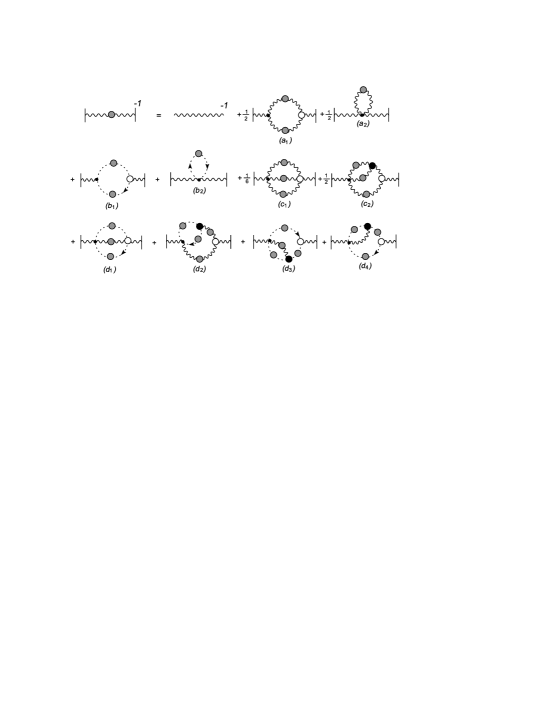
Figure 1: The SD equation for the gluon propagator. Wavy lines with grey blobs represent full-quantum gluon propagators, while the dashed lines with grey blobs denote full-ghost propagators. All external wavy lines (ending with a vertical line) are background gluons. The black dots are the tree-level vertices in the BFM, while black blob represents the full conventional vertices. The white blobs denote three or four-gluon vertices with one external background leg.

As is widely known, in the conventional formalism the inclusion of ghosts is instrumental for the transversality of $\Pi^{ab}_{\mu\nu}(q)$, already at the level of the one-loop calculation. On the other hand, in the PT-BFM formalism, due to new Feynman rules for the vertices, the one-loop gluon and ghost contribution are individually transverse Abbott:1980hw .

As has been shown in Aguilar:2006gr , this crucial feature persists at the non-perturbative level, as a consequence of the simple WIs satisfied by the full vertices appearing in the diagrams of Fig.(1). Specifically, the gluonic and ghost sector are separately transverse, within each individual order in the dressed-loop expansion

We will show this property for the one-loop dressed terms. We start by writing down the fundamental all-order WI for the full three-gluon vertex with one background gluon, ${\widetilde{{\rm I}\Gamma}}_{\mu\alpha\beta}^{abc}$, and for the full background gluon-ghost vertex ${\widetilde{{\rm I}\Gamma}}_{\mu}^{acb}$,

$$q_{1}^{\mu}{\widetilde{{\rm I}\Gamma}}_{\mu\alpha\beta}^{abc}(q_{1},q_{2},q_{3}) = gf^{abc}\left[\Delta^{-1}_{\alpha\beta}(q_{2})-\Delta^{-1}_{\alpha\beta}(q_{3})\right]\,,$$

$$q_{1}^{\mu}{\widetilde{{\rm I}\Gamma}}_{\mu}^{acb}(q_{2},q_{1},q_{3}) = gf^{abc}\left[D^{-1}(q_{2})-D^{-1}(q_{3})\right]\,,$$ (4)

where on the RHS we have differences of inverse of the quantum gluon, $\Delta_{\mu\nu}(q)$, and ghost, $D(q)$, propagators.

The closed expressions corresponding to the gluonic sector, at one-loop dressed expansion, (see Fig.(1)) are given by

$$\widehat{\Pi}^{ab}_{\mu\nu}(q)\big{|}_{{\bf a_{1}}} = \frac{1}{2}\,\int\!\![dk]\,\widetilde{\Gamma}_{\mu\alpha\beta}^{aex}\Delta^{\alpha\rho}_{ee^{\prime}}(k){\widetilde{{\rm I}\Gamma}}_{\nu\rho\sigma}^{be^{\prime}x^{\prime}}\Delta^{\beta\sigma}_{xx^{\prime}}(k+q)\,,$$

$$\widehat{\Pi}^{ab}_{\mu\nu}(q)\big{|}_{{\bf a_{2}}} = \frac{1}{2}\,\int\!\![dk]\,\widetilde{\Gamma}_{\mu\nu\alpha\beta}^{abex}\Delta^{\alpha\beta}_{ex}(k)\,,$$ (5)

with $\widetilde{\Gamma}_{\mu\alpha\beta}^{aex}$ and $\widetilde{\Gamma}_{\mu\nu\alpha\beta}^{abex}$ being the three and four bare gluon vertices in the Feynman gauge of the BFM Abbott:1980hw .

For the ghost sector, we have

$$\widehat{\Pi}^{ab}_{\mu\nu}(q)\big{|}_{{\bf b_{1}}} = -\,\int\!\![dk]\,\widetilde{\Gamma}_{\mu}^{aex}D_{ee^{\prime}}(k){\widetilde{{\rm I}\Gamma}}_{\nu}^{be^{\prime}x^{\prime}}D_{xx^{\prime}}(k+q)\,,$$

$$\widehat{\Pi}^{ab}_{\mu\nu}(q)\big{|}_{{\bf b_{2}}} = -\int\!\![dk]\,\,\widetilde{\Gamma}_{\mu\nu}^{abex}D_{ex}(k)\,.$$ (6)

where $\widetilde{\Gamma}_{\mu}^{aex}$ and $\widetilde{\Gamma}_{\mu\nu}^{abex}$ represent the tree-level ghost-gluon vertices with one (two) background gluon(s) respectively Abbott:1980hw ; the measure $[dk]=d^{d}k/(2\pi)^{d}$   with $d=4-\epsilon$ the dimension of space-time. Observe that in our notation all the three and four-point functions with a tilde are vertices with at least one external (background) gluon leg.

With the above WI we can prove that the groups (a) and (b) are independently transverse. We start with group (a)

$$q^{\nu}\widehat{\Pi}^{ab}_{\mu\nu}(q)\big{|}_{{\bf a_{1}}} = C_{A}\,g^{2}\delta^{ab}\,q_{\mu}\,\int\!\![dk]\,\Delta^{\rho}_{\rho}(k)\,,$$

$$q^{\nu}\widehat{\Pi}^{ab}_{\mu\nu}(q)\big{|}_{{\bf a_{2}}} = -C_{A}\,g^{2}\delta^{ab}\,q_{\mu}\,\int\!\![dk]\,\Delta^{\rho}_{\rho}(k)\,,$$ (7)

and thus

$$q^{\nu}\left(\widehat{\Pi}^{ab}_{\mu\nu}(q)\big{|}_{{\bf a_{1}}}+\widehat{\Pi}^{ab}_{\mu\nu}(q)\big{|}_{{\bf a_{2}}}\right)=0\,.$$ (8)

Similarly, the one-loop-dressed ghost contributions give upon contraction

$$q^{\nu}\widehat{\Pi}^{ab}_{\mu\nu}(q)\big{|}_{{\bf b_{1}}} = 2\,C_{A}\,g^{2}\delta^{ab}\,q_{\nu}\,\int\!\![dk]\,D(k)\,,$$

$$q^{\nu}\widehat{\Pi}^{ab}_{\mu\nu}(q)\big{|}_{{\bf b_{2}}} = -2\,C_{A}\,g^{2}\delta^{ab}\,q_{\nu}\,\int\!\![dk]\,D(k)\,,$$ (9)

and so

$$q^{\nu}\left(\widehat{\Pi}^{ab}_{\mu\nu}(q)\big{|}_{{\bf b_{1}}}+\widehat{\Pi}^{ab}_{\mu\nu}(q)\big{|}_{{\bf b_{2}}}\right)=0\,.$$ (10)

The proof of the individual transversality of the groups (c) and (d), constituting the two-loop dressed expansion of $\widehat{\Pi}_{\mu\nu}(q)$, is slightly more cumbersome but essentially straightforward Aguilar:2006gr .

The importance of this transversality property in the context of SD equation is that it allows for a meaningful first approximation: instead of the system of coupled equations involving gluon and ghost propagators, one may consider only the subset containing gluons, without compromising the crucial property of transversality. More generally, one can envisage a systematic dressed loop expansion, maintaining transversality manifest at every level of approximation. This is not to say, of course, that we have some a-priori guarantee that the subset of diagrams considered here is numerically dominant. Actually, as has been argued in a series of SD studies, in the context of the conventional Landau gauge it is the ghost sector that furnishes in fact the leading contribution vonSmekal:1997is Clearly, it is plausible that this characteristic feature may persist within the PT-BFM scheme as well, and we will explore this crucial issue in the near future

Thus, in this formalism, the first non-trivial approximation for $\widehat{\Delta}^{-1}(q^{2})$ that preserves its transversality is given by the gluonic terms of the one-loop expansion (diagrams ($a_{1}$) and ($a_{2}$) in Fig.(1)), written in closed form in Eq. (5).

However, the equation given in (5) is not a genuine SD equation, in the sense that it does not involve the unknown quantity $\widehat{\Delta}$ on both sides; instead, in the integrals of the RHS appears $\Delta$. Replacing $\Delta$ by $\widehat{\Delta}$ is a highly non-trivial proposition, whose self-consistency is still an open issue. Its implementation may be systematized by resorting to a set of crucial identities relating $\Delta$ and $\widehat{\Delta}$ by means of a set of auxiliary Green’s functions involving anti-fields and background sources. At this point we will assume that to a first approximation one may neglect the effects of the aforementioned auxiliary Green’s functions, and carry out the substitution $\Delta\to\widehat{\Delta}$ on the RHS of (5). Hence, the SD equation we will solve is written as

$$\widehat{\Delta}^{-1}(q^{2})=q^{2}+i\left[\widehat{\Pi}^{(\bf{a_{1}})}(q^{2})+\widehat{\Pi}^{(\bf{a_{2}})}\right]\,,$$ (11)

where

$$\widehat{\Pi}_{\mu\nu}^{(\bf{a_{1}})}(q) = \frac{1}{2}\,C_{A}\,g^{2}\,\int\!\![dk]\widetilde{\Gamma}_{\mu\alpha\beta}\widehat{\Delta}^{\alpha\alpha^{\prime}}(k){\widetilde{{\rm I}\Gamma}}_{\nu\alpha^{\prime}\beta^{\prime}}\widehat{\Delta}^{\beta\beta^{\prime}}(k+q)\,,$$

$$\widehat{\Pi}_{\mu\nu}^{(\bf{a_{2}})} = -C_{A}\,g^{2}\,g_{\mu\nu}\int\!\![dk]\widehat{\Delta}(k)\,.$$ (12)

With the above equation at hand, we proceed to establish the conditions necessary for obtaining infrared finite solutions for $\widehat{\Delta}^{-1}(q^{2})$, i.e. solutions for which $\widehat{\Delta}^{-1}(0)\neq 0$. There are two such conditions: one must (i) allow for non-vanishing seagull-like contribution, and (ii) introduce massless poles into the Ansatz for the full three-gluon vertex.

The necessity of the first condition can be appreciated by observing that, on dimensional grounds, the value of $\widehat{\Delta}^{-1}(0)$ can only be proportional to two types of seagull-like contributions,

$${\cal T}_{0}=\int\!\,[dk]\,\widehat{\Delta}(k),\qquad{\cal T}_{1}=\int\!\,[dk]\,k^{2}\,\widehat{\Delta}^{2}(k)\,,$$ (13)

since, inside the diagrams of Eq.(12), there can be at most two full gluon self-energies, $\widehat{\Delta}$. However, it is well known that, due to the dimensional regularization rules, such contributions vanish perturbatively, ensuring the masslessness of the gluon order by order in perturbation theory. In order for finite solutions to emerge, one must assume that seagull-like contributions, such as those of Eq.(13), do not vanish non-perturbatively. Naturally, this last step will force us to deal with the quadratic divergences, present in both integrals of Eq.(13), and therefore a suitable regularization scheme must be subsequently employed.

Allowing the non-vanishing of seagull-like terms is not the whole story however; one must determine in addition the mechanism that will produce their appearance. One thing is certain: the seagull contributions determining $\widehat{\Delta}^{-1}(0)$ do not originate from diagram $(a_{2})$ in Fig.(1). Instead, the required seagull contributions will stem from diagram $(a_{1})$, after the inclusion of massless poles into the Ansatz for the full three-gluon vertex $\widetilde{{\rm I}\Gamma}$. Diagram $(a_{2})$ plays of course a crucial role in enforcing the transversality of $\widehat{\Pi}_{\mu\nu}$ non-perturbatively, but in the absence of massless poles in the vertex one would still get $\widehat{\Delta}^{-1}(0)=0$.

There is a relatively simple argument that amply demonstrates the subtle interplay between both requirements. Specifically, $i\widehat{\Pi}_{\mu\nu}^{(\bf{a_{1}})}(q)$ can be written in the general form

$$i\widehat{\Pi}_{\mu\nu}^{(\bf{a_{1}})}(q)=q^{2}A(q^{2})g_{\mu\nu}+B(q^{2})q_{\mu}q_{\nu}\,,$$ (14)

where $A(q^{2})$ and $B(q^{2})$ are arbitrary dimensionless functions, whose precise expressions depend on the details of the ${\widetilde{{\rm I}\Gamma}}_{\nu\alpha^{\prime}\beta^{\prime}}$ employed. The transversality of $i\left[\widehat{\Pi}_{\mu\nu}^{(\bf{a_{1}})}(q)+\widehat{\Pi}_{\mu\nu}^{(\bf{a_{2}})}\right]$ implies immediately the condition

$$q^{2}\left[A(q^{2})+B(q^{2})\right]=iC_{A}\,g^{2}\,{\cal T}_{0}\,,$$ (15)

and thus the sum of the two graphs reads

$$i\left[\widehat{\Pi}_{\mu\nu}^{(\bf{a_{1}})}(q)+\widehat{\Pi}_{\mu\nu}^{(\bf{a_{2}})}\right]=-q^{2}B(q^{2})P_{\mu\nu}(q)\,.$$ (16)

Clearly from Eq.(11), we conclude that $\widehat{\Delta}^{-1}(0)={\displaystyle\lim_{q^{2}\to 0}}(-q^{2}B(q^{2}))$.

Interestingly enough, once the transversality of $\widehat{\Pi}_{\mu\nu}$ has been enforced, the value of $\widehat{\Delta}^{-1}(0)$ is determined solely by ${\displaystyle\lim_{q^{2}\to 0}}\left(-q^{2}B(q^{2})\right)$. Evidently, if $B(q^{2})$ does not contain $(1/q^{2})$ terms, one has that ${\displaystyle\lim_{q^{2}\to 0}}(-q^{2}B(q^{2}))=0$, and therefore $\widehat{\Delta}^{-1}(0)=0$, despite the fact that ${\cal T}_{0}$ has been assumed to be non-vanishing. Thus, if the full three-gluon vertex $\widetilde{{\rm I}\Gamma}$ satisfies the WI of (4), but does not contain poles, then the seagull contribution ${\cal T}_{0}\neq 0$ of graph ($a_{2}$) will cancel exactly against analogous contributions contained in graph ($a_{1}$), forcing $\widehat{\Delta}^{-1}(0)=0$.

We next proceed to study the SD of Eq.(11). We will follow the methodology developed in Cornwall:1982zr and linearize the equation by resorting to the Lehmann representation, together with a gauge-technique inspired Ansatz for the vertex ${\widetilde{{\rm I}\Gamma}}_{\nu\alpha\beta}$. This approximation yields a more tractable form for the resulting SD equation, which for the purposes of this preliminary analysis should suffice; of course, a non-linear study must eventually be carried out, and lies within our immediate plans.

To simplify the form of the vertex required, we drop the longitudinal parts of $\widehat{\Delta}_{\mu\nu}$ inside the integrals, using $\widehat{\Delta}_{\mu\nu}(k)=-ig_{\mu\nu}\widehat{\Delta}(k)$. Omitting these terms does not interfere with the transversality of the external $\widehat{\Delta}_{\mu\nu}(q)$ Aguilar:2006gr . Then we obtain

$$\widehat{\Pi}_{\mu\nu}(q) = \frac{1}{2}\,C_{A}\,g^{2}\,\int\![dk]\,\widetilde{\Gamma}_{\mu}^{\alpha\beta}\widehat{\Delta}(k){\widetilde{{\rm I}\Gamma}}_{\nu\alpha\beta}\widehat{\Delta}(k+q)$$ (17)

$$- \,C_{A}\,g^{2}\,\,d\,g_{\mu\nu}\int\![dk]\,\widehat{\Delta}(k)\,,$$

with

$$\widetilde{\Gamma}_{\mu\alpha\beta}=(2k+q)_{\mu}g_{\alpha\beta}-2q_{\alpha}g_{\mu\beta}+2q_{\beta}g_{\mu\alpha}\,,$$ (18)

and

$$q^{\nu}{\widetilde{{\rm I}\Gamma}}_{\nu\alpha\beta}=\left[\widehat{\Delta}^{-1}(k+q)-\widehat{\Delta}^{-1}(k)\right]g_{\alpha\beta}\,.$$ (19)

The Lehmann representation for the scalar part of the gluon propagator reads

$$\widehat{\Delta}(q^{2})=\int\!\!d\lambda^{2}\,\frac{\rho\,(\lambda^{2})}{q^{2}-\lambda^{2}+i\epsilon}\,,$$ (20)

with no special assumptions on the form of the spectral density.

This way of writing $\widehat{\Delta}(q^{2})$ allows for a relatively simple gauge-technique Ansatz for ${\widetilde{\Gamma}^{\rm L}_{\nu\alpha\beta}}$, which linearizes the resulting SDE. In particular, setting on the first integral of the RHS of Eq.(17)

$$\widehat{\Delta}(k)\,{\widetilde{{\rm I}\Gamma}}_{\nu\alpha\beta}\,\widehat{\Delta}(k+q)=\int\!\!d\lambda^{2}\,\rho\,(\lambda^{2})\frac{1}{k^{2}-\lambda^{2}+i\epsilon}\,{\widetilde{\Gamma}^{\rm L}_{\nu\alpha\beta}}\,\frac{1}{(k+q)^{2}-\lambda^{2}+i\epsilon}\,,$$ (21)

where ${\widetilde{\Gamma}^{\rm L}_{\nu\alpha\beta}}$ must be such as to satisfy the tree-level WI

$$q^{\nu}{\widetilde{\Gamma}^{\rm L}_{\nu\alpha\beta}}=\left[(k+q)^{2}-k^{2}\right]g_{\alpha\beta}=\left[(k+q)^{2}-\lambda^{2}\right]g_{\alpha\beta}-(k^{2}-\lambda^{2})g_{\alpha\beta}\,.$$ (22)

Then, it is straightforward to show by contracting both sides of (21) with $q^{\nu}$, and employing (20) and (22), that ${\widetilde{\Gamma}^{\rm L}_{\nu\alpha\beta}}$ satisfies the all-order WI of Eq.(19). Of course, choosing ${\widetilde{\Gamma}^{\rm L}_{\nu\alpha\beta}}=\widetilde{\Gamma}_{\nu\alpha\beta}$ solves the WI, but as we will see in detail in what follows, due to the absence of pole terms, it does not allow for mass generation, in accordance with our previous discussion. Instead we propose the following form for the vertex

$${\widetilde{\Gamma}^{\rm L}_{\nu\alpha\beta}}=\widetilde{\Gamma}_{\nu\alpha\beta}+c_{1}\left((2k+q)_{\nu}+\frac{q_{\nu}}{q^{2}}\left[k^{2}-(k+q)^{2}\right]\right)g_{\alpha\beta}+\left(c_{3}+\frac{c_{2}}{2\,q^{2}}\left[(k+q)^{2}+k^{2}\right]\right)\left(q_{\beta}g_{\nu\alpha}-q_{\alpha}g_{\nu\beta}\right),\,$$ (23)

which, due to the presence of the massless pole is expected to allow the possibility of infrared finite solution. Furthermore, we treat the constants $c_{1}$, $c_{2}$ and $c_{3}$ as arbitrary parameters, in order to check quantitatively the sensitivity of the obtained solutions on the specific details of the form of the vertex. Notice that all new terms contributing to ${\widetilde{\Gamma}^{\rm L}_{\nu\alpha\beta}}$ have the correct properties under Bose symmetry.

Thus, the vertex ${\widetilde{{\rm I}\Gamma}}$ entering in Eq.(12), can be obtained as a combination of Eqs.(21) and (23). After rather lengthy algebraic manipulations of Eq.(11) (see Aguilar:2006gr for details), fixing $c_{3}=\frac{1}{3}c_{1}$ to recover the perturbative result, we obtain for the renormalized $\widehat{\Delta}(q^{2})$ (in the Euclidean space)

$${\widehat{\Delta}}^{-1}(q^{2})=q^{2}\Bigg{\{}K+{\tilde{b}}\,g^{2}\int^{q^{2}/4}_{0}\!\!\!dz\,\left(1-\frac{4z}{q^{2}}\right)^{1/2}\,{\widehat{\Delta}}(z)\Bigg{\}}+\,\gamma{\tilde{b}}g^{2}\int^{q^{2}/4}_{0}\!\!\!dz\,z\,\left(1-\frac{4z}{q^{2}}\right)^{1/2}\widehat{\Delta}(z)\,\,+{\widehat{\Delta}}^{-1}(0)\,,$$ (24)

with ${\tilde{b}}=10\,C_{A}/48\pi^{2}$,

$$\widehat{\Delta}^{-1}(0)=-\frac{{\tilde{b}}g^{2}\sigma}{\pi^{2}}\int\!d^{4}k\,\widehat{\Delta}(k^{2})\,,$$ (25)

and

$$\sigma\,\equiv\,\frac{6\,(c_{1}+c_{2})}{5}\,,\,\,\,\,\,\,\,\,\gamma\,\equiv\,\frac{4+4\,c_{1}+3\,c_{2}}{5}\,.$$ (26)

The renormalization constant $K$ is to be fixed by the condition, ${\widehat{\Delta}}^{-1}(\mu^{2})=\mu^{2}$, with $\mu^{2}\gg\Lambda^{2}$. Notice that the deviation of ${\tilde{b}}$ from the value $b=11\,C_{A}/48\pi^{2}$, the standard coefficient of the one-loop $\beta$ function of QCD, is due to the omission of the ghosts. From (25) it is clear that when $\sigma=0$ automatically $\widehat{\Delta}^{-1}(0)$ vanishes, despite the inclusion of ($a_{2}$). Note however that having poles is not a sufficient condition: if $c_{1}=-c_{2}$, there is no effect.

It is interesting to study the UV behavior for ${\widehat{\Delta}}(q^{2})$ predicted by the integral equation (24). At large $q^{2}$ we can safely replace the factors $(1-4z/q^{2})^{1/2}\to 1$, arriving at the following simplified version of that equation,

$$\widehat{\Delta}^{-1}(q^{2})=q^{2}\left(1+{\tilde{b}}g^{2}\int^{q^{2}}_{\mu^{2}}\!\!\!dz\,\widehat{\Delta}(z)\right)\,,$$ (27)

whose solution can be easily obtained by casting it into an differential equation, written in terms of the form factor $G(q^{2})=q^{2}\widehat{\Delta}(q^{2})$, which lead us to

$$\widehat{\Delta}^{-1}(q^{2})=q^{2}\left[1+2{\tilde{b}}g^{2}\ln\left(\frac{q^{2}}{\mu^{2}}\right)\right]^{1/2}\,.$$ (28)

Obviously, upon expansion this expression recovers the one-loop result ${\widehat{\Delta}}^{-1}(q^{2})|_{pert}=q^{2}\left(1+{\tilde{b}}\,g^{2}\ln(q^{2}/\mu^{2})\right)$ correctly, but ${\widehat{\Delta}}(q^{2})$ does not display the expected RG behavior at higher order. The fundamental reason for this discrepancy can be essentially traced back to having carried out the renormalization subtractively instead of multiplicatively Cornwall:1982zr ; Cornwall:1985bg , a fact that distorts the RG structure of the equation.

As is well-known, due to the Abelian WI satisfied by the PT effective Green’s functions, $\widehat{\Delta}^{-1}(q^{2})$ absorbs all the RG-logs, exactly as happens in QED with the photon self-energy. Consequently, the product ${\widehat{d}}(q^{2})=g^{2}\widehat{\Delta}(q^{2})$ should form a RG-invariant ($\mu$-independent) quantity. Notice however that Eq.(24) does not encode the correct RG behavior: when written in terms of the RG invariant quantity $\widehat{d}(q^{2})=g^{2}\widehat{\Delta}(q^{2})$ it is not manifestly $g^{2}$-independent, as it should.

In order to restore the correct RG behavior at the level of (24), observe that such equation requires an extra power of $g^{2}$ in their integrands on the RHS. Then, we use the simple prescription whereby we substitute every $\widehat{\Delta}(z)$ appearing on RHS of Eq.(24) by Cornwall:1982zr ; Cornwall:1985bg

$$\widehat{\Delta}(z)\to\frac{g^{2}\,\widehat{\Delta}(z)}{\bar{g}^{2}(z)}\equiv[1+\tilde{b}g^{2}\ln(z/\mu^{2})]\widehat{\Delta}(z)\,.$$ (29)

which allows us to cast Eq.(24) in terms of the RG-invariant quantities $\widehat{d}(q^{2})$ and $\bar{g}^{2}(q^{2})$ in the following way:

$${\widehat{d}}^{\,-1}(q^{2}) = q^{2}\Bigg{\{}\frac{1}{g^{2}}+{\tilde{b}}\Bigg{(}\int^{q^{2}/4}_{0}\!dz\,\left(1-\frac{4z}{q^{2}}\right)^{1/2}\frac{{\widehat{d}}(z)}{\bar{g}^{2}(z)}-\int^{\mu^{2}/4}_{0}\!dz\,\left(1-\frac{4z}{\mu^{2}}\right)^{1/2}\,\frac{{\widehat{d}}(z)}{\bar{g}^{2}(z)}\Bigg{)}\Bigg{\}}$$ (30)

$$+ \,\gamma{\tilde{b}}\Bigg{(}\int^{q^{2}/4}_{0}\!dz\,z\,\left(1-\frac{4z}{q^{2}}\right)^{1/2}\frac{{\widehat{d}}(z)}{\bar{g}^{2}(z)}\,\,-\frac{q^{2}}{\mu^{2}}\int^{\mu^{2}/4}_{0}\!dz\,z\left(1-\frac{4z}{\mu^{2}}\right)^{1/2}\,\frac{{\widehat{d}}(z)}{\bar{g}^{2}(z)}\Bigg{)}+{\widehat{d}}^{\,-1}(0)\;,$$

where

$${\widehat{d}}^{\,-1}(0)=-\frac{{\tilde{b}}\sigma}{\pi^{2}}\int\!d^{4}k\,\frac{{\widehat{d}}(k^{2})}{\bar{g}^{2}(k^{2})}\,.$$ (31)

It is easy to see now that Eq.(30) yields the correct UV behavior, i.e. ${\widehat{d}}^{\,-1}(q^{2})=\tilde{b}\,q^{2}\ln(q^{2}/\Lambda^{2})$.

When solving (30) we will be interested in solutions that are qualitatively of the general form

$${\widehat{d}}(q^{2})=\frac{{\overline{g}}^{2}_{{{\scriptscriptstyle\rm NP}}}(q^{2})}{q^{2}+m^{2}(q^{2})}\,,$$ (32)

where

$${\overline{g}}^{2}_{{{\scriptscriptstyle\rm NP}}}(q^{2})=\bigg{[}\tilde{b}\ln\left(\frac{q^{2}+f(q^{2},m^{2}(q^{2}))}{\Lambda^{2}}\right)\bigg{]}^{-1}\,,$$ (33)

The quantity ${\overline{g}}^{2}_{{{\scriptscriptstyle\rm NP}}}(q^{2})$ represents a non-perturbative version of the RG-invariant effective charge of QCD: in the deep UV it goes over to $\overline{g}^{2}(z)$, while in the deep IR it will be finite due to the presence of the function $f(q^{2},m^{2}(q^{2}))$, whose form will be determined by fitting the numerical solution.

The function $m^{2}(q^{2})$ may be interpreted as a momentum dependent “mass”. On general arguments dynamically generated masses must vanish asymptotically. In order to determine the asymptotic behavior that Eq.(30) predicts for $m^{2}(q^{2})$ at large $q^{2}$, we replace Eq.(32) on both sides of Eq.(30), set $(1-4z/q^{2})^{1/2}\to 1$, and demand the consistency of both sides, obtaining finally

$$m^{2}(q^{2})\sim m^{2}_{0}\ln^{-a}\left(q^{2}/\Lambda^{2}\right)\,,\quad\mbox{with}\quad a=1+\gamma\,.$$ (34)

Indeed the gluon mass vanishes at UV as an inverse power of $\ln(q^{2})$, since $a>0$. Actually, as we will see below, the regularization of Eq.(31) imposes a more stringent constraint, requiring that $\gamma>0$, thus restricting through Eq.(26) the possible values of $c_{1}$ and $c_{2}$ in ${\widetilde{\Gamma}^{\rm L}_{\nu\alpha\beta}}$.

As mentioned before, the seagull-like contribution (denoted collectively by ${\widehat{d}}^{\,-1}(0)$ in Eq.(30)) are essential for obtaining IR finite solution for ${\widehat{d}}(q^{2})$. However, the integral (31) should be properly regularized, in order to ensure the finiteness of such a mass term.

For the regulation of the quadratic divergences present in the integral (31), we rely on two basic ingredients: (i) the standard integration rules of the dimensional regularization and (ii) a constraint on the allowed values of the anomalous mass-dimension $a$.

With this in mind, we recall that according to the dimensional regularization rules, $\int\!\,[dk]/k^{2}=0$, allowing us to rewrite the Eq.(31) (using (32)) as

$${\widehat{d}}^{\,-1}(0) \equiv -\frac{{\tilde{b}}\sigma}{\pi^{2}}\int\![dk]\bigg{(}\,\frac{{\overline{g}}^{2}_{{{\scriptscriptstyle\rm NP}}}(k^{2})}{[k^{2}+m^{2}(k^{2})]\bar{g}^{2}(k^{2})}-\frac{1}{k^{2}}\bigg{)}$$ (35)

$$=\frac{{\tilde{b}}\sigma}{\pi^{2}}\int\![dk]\frac{m^{2}(k^{2})}{k^{2}\,[k^{2}+m^{2}(k^{2})]}\,$$

$$+\frac{{\tilde{b}^{2}}\sigma}{\pi^{2}}\int\![dk]\,{\widehat{d}}(k^{2})\,\ln\left(1+\frac{f(k^{2},m^{2}(k^{2}))}{k^{2}}\right)\,.$$

The inspection of the two integrals on the RHS separately reveals that, if $m^{2}(k^{2})$ falls asymptotically as power of $\ln^{-a}(k^{2})$, with $a>1$, then the first integral would converge, by virtue of the elementary result

$$\int\frac{dz}{z\,(\ln z)^{1+\gamma}}=-\frac{1}{\gamma\,(\ln z)^{\gamma}}\,,$$ (36)

which, of course, requires that $\gamma>0$. The second integral will converge as well, provided that $f(k^{2},m^{2}(k^{2}))$ drops asymptotically at least as fast as $\ln^{-c}(k^{2})$, with $c>0$. If, for example, $f=\rho m^{2}(k^{2})$ (with $1+\gamma>1$, for the first integral to converge), then the convergence condition for the second integral is automatically fulfilled. Notice that perturbatively ${\widehat{d}}^{\,-1}(0)$ vanishes; this is because $m^{2}(k^{2})=0$ to all orders, and therefore, since in that case also $f=0$, both integrals on the RHS of (35) vanish.

Evidently, Eqs.(30) and (35) form a system of equation; the role of the first is to provide a solution for the unknown RGI quantity, ${\widehat{d}}(q^{2})$, while the second acts as an additional constraint, restricting the number of possible solutions. Therefore, Eqs.(30) and (35) should be solved simultaneously.

Using an iterative method, we performed a detailed study of these two equations, where for each ${\widehat{d}}^{-1}(0)$ chosen we vary $\gamma$ and $\sigma$ in order to scan the two-parameter space of solutions.

In Fig.(2), we show numerical results for ${\widehat{d}}(q^{2})$, for different values of ${\widehat{d}}^{\,-1}(0)$. All these solutions satisfy the constraint imposed by Eq.(35) and their respective values for $\sigma$ are described in the inserted legend. As expected, the gluon propagator behaves at low momenta like a constant, whose value is determined by ${\widehat{d}}(0)$; in addition, it obeys the correct ultraviolet behavior. As can be observed from the plot, ${\widehat{d}}(q^{2})$ starts off as constant until the neighborhood of $q^{2}=0.01\;\mbox{GeV}^{\,2}$, where the curve bends downward in order to match with the perturbative asymptotic behavior at a scale of a few $\mbox{GeV}^{\,2}$. All these solutions can be perfectly fitted by Eq.(32); the functional form of $f(q^{2},m^{2}(q^{2}))$ and $m^{2}(q^{2})$ that better describe our data sets are given by

$$f(q^{2},m^{2}(q^{2}))=\rho_{\,1}m^{2}(q^{2})+\rho_{\,2}\frac{m^{4}(q^{2})}{q^{2}+m^{2}(q^{2})}\,,$$ (37)

and the dynamical mass,

$$m^{2}(q^{2})=m^{2}_{0}\left[\ln\left[\frac{q^{2}+\rho_{\,1}\,m^{2}_{0}}{\Lambda^{2}}\right]\Big{/}\ln\left[\frac{\rho_{\,1}\,m^{2}_{0}}{\Lambda^{2}}\right]\right]^{-a}\,,$$ (38)

with exponent $a=1+\gamma$.

In all cases, we fixed $\rho_{1}=4$; therefore, the unique free parameter is $\rho_{\,2}$, since the value of $m^{2}_{0}$, which is also related to $\rho_{\,2}$, can be directly obtained by setting $q^{2}=0$ in Eq.(32). From this follows immediately that the value of the infrared fixed point of the running coupling, ${\overline{g}}^{\,-2}_{{{\scriptscriptstyle\rm NP}}}(0)$ will be determined by the value assumed by $f(0,m^{2}_{0})$, since

$${\overline{g}}^{\,-2}_{{{\scriptscriptstyle\rm NP}}}(0)=\tilde{b}\ln\left[\frac{(4+\rho_{\,2})\,m^{2}_{0}}{\Lambda^{2}}\right]\,.$$ (39)

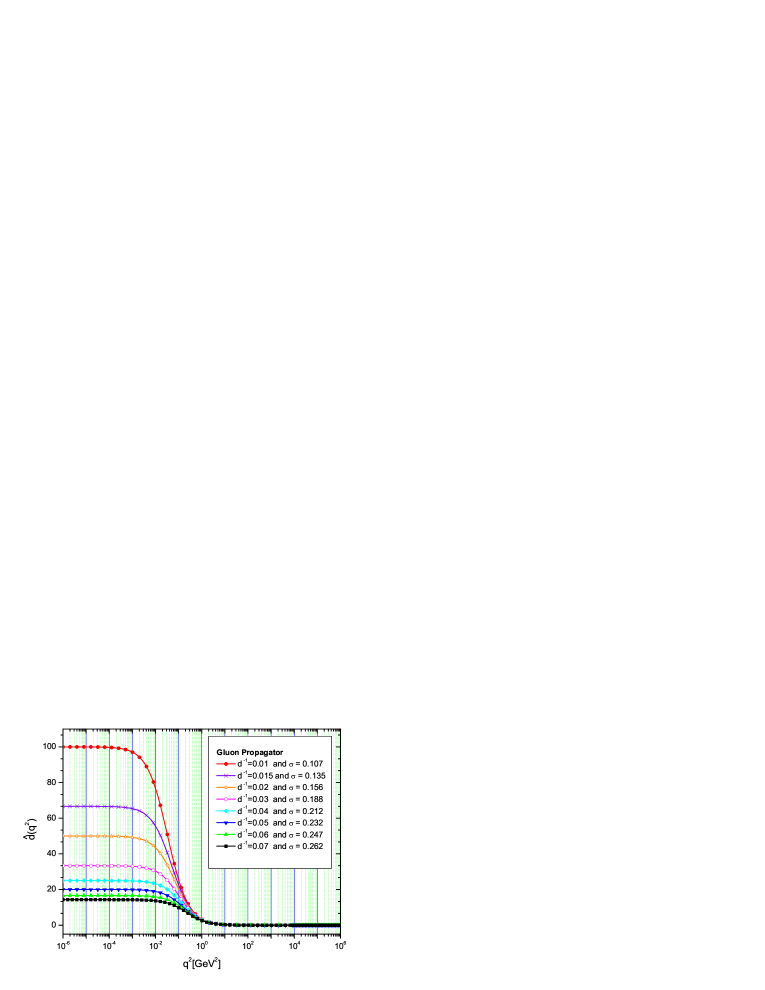
Figure 2: Results for ${\widehat{d}}(q^{2})$ fixing different values for ${\widehat{d}}^{\,-1}(0)$ (all in $\;\mbox{GeV}^{\,2}$). All these solutions satisfy the condition given by Eq.(35). Their respective values for $\sigma$ are given in the legend, in all cases we set $c_{2}=0$ in Eq.(26).

Figure 3: The running charge, $\alpha(q^{2})$, corresponding to the gluon propagator of Fig.(2). Clearly, $\alpha(0)$ increases as ${\widehat{d}}^{\,-1}(0)$ decreases

Obviously, the maximum value obtained for ${\overline{g}}^{2}_{{{\scriptscriptstyle\rm NP}}}(0)$, is the one that minimizes $(4+\rho_{\,2})\,m^{2}_{0}$ and, at same time, keeps it bigger than $\Lambda^{2}$, in order to avoid the pole. Of course, if we set $\rho_{\,2}=0$ in Eq.(37), we automatically recover the solution proposed in Cornwall:1982zr ; however our numerical solution requires bigger values for the coupling ${\overline{g}}^{2}_{{{\scriptscriptstyle\rm NP}}}(q^{2})$, and therefore $\rho_{\,2}$ assumes negative values, as can be observed on Fig.(3)

The running charges, $\alpha(q^{2})$, for each solution presented on Fig.(2) are displayed in Fig.(3). Observe that as the value of ${\widehat{d}}^{\,-1}(0)$ decreases, the value of the infrared fixed point of the running coupling, $\alpha(0)$, increases. Accordingly, from Fig.(2) and Fig.(3), we can conclude that, if smaller values of $\sigma$ were to be favored by QCD, the freezing of the running coupling would occur at higher values. It should also be noted that the values of $\alpha(0)$ found here tend to be slightly more elevated compared to those of Cornwall:1982zr (for the same value of $m^{2}_{0}$) .

Finally, we analyze the dependence of the ratio $m_{0}/\Lambda$ on $\sigma$; the former is extracted from Eq.(32) by setting $q^{2}=0$. This dependence is shown in the Fig.(4), corresponding to the cases presented in Fig.(2). We observe that as we increase the value of $\sigma$, namely the sum of the coefficients of the massless pole terms appearing in the three gluon vertex, the ratio $m_{0}/\Lambda$ grows exponentially.

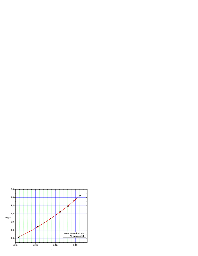
Figure 4: The ratio $m_{0}/\Lambda$ as function of the parameter $\sigma$. The increase is exponential, given by $m_{0}/\Lambda=A_{1}\exp(\sigma/t_{1})+y_{0}$, where $A_{1}=0.775$, $t_{1}=0.25$ and $y_{0}=0.436$.

In conclusion, we have presented an analysis of the various intertwined issues involved in the study of dynamical gluon mass generation through SD equations. The analysis was carried out in the context of the PT-BFM scheme, where various crucial properties are preserved manifestly. Most notably, the transversality of the non-perturbative gluon self-energy is enforced order by order in the dressed loop expansion and separately for gluons and ghost. We have seen in detail that for the existence of infrared finite solutions two requirements are indispensable: (i) the non-vanishing of seagull-like contributions beyond perturbation theory, and (ii) the presence of massless poles in the trilinear gluon vertex. The resulting equation was linearized by resorting to the Lehmann representation and a gauge-technique inspired solution of the corresponding WI. A simple Ansatz for the three-gluon vertex was constructed, which contains massless poles, thus allowing for the appearance of infrared finite solutions. This vertex satisfies the correct WI, but otherwise is purely phenomenological, in the sense that it is not QCD-derived, nor does it contain the most general Lorentz structure. Numerical solutions were obtained for the RG-invariant quantity ${\widehat{d}}(q^{2})$; they can be fitted perfectly by means of a running coupling that freezes in the IR, and a dynamical mass that vanishes in the UV. We have found that the actual values of $\alpha(0)$ depend strongly on the combined strength of the pole terms appearing in the vertex. This strongly suggests that the value of this IR fixed point should be determined by means of a detailed non-perturbative study of the three-gluon vertex, either on the lattice or through its own SD equation. Needless to say, many of the issues considered in this talk are far from settled, and a lot of independent work is necessary before reaching definite conclusions.

References

• (1) J. M. Cornwall, Phys. Rev. D 26, 1453 (1982).
• (2) J. M. Cornwall and J. Papavassiliou, Phys. Rev. D 40, 3474 (1989).
• (3) L. F. Abbott, Nucl. Phys. B 185, 189 (1981).
• (4) D. Binosi and J. Papavassiliou, Phys. Rev. D 66, 111901 (2002); J. Phys. G 30, 203 (2004).
• (5) A. C. Aguilar and J. Papavassiliou, arXiv:hep-ph/0610040.
• (6) L. von Smekal, R. Alkofer and A. Hauck, Phys. Rev. Lett.  79, 3591 (1997); R. Alkofer and L. von Smekal, Phys. Rept.  353, 281 (2001); C. S. Fischer, J. Phys. G 32, R253 (2006); C. S. Fischer and J. M. Pawlowski, arXiv:hep-th/0609009.
• (7) J. M. Cornwall and W. S. Hou, Phys. Rev. D 34, 585 (1986).