Relativistic NJL Model with Light and Heavy Quarks

Abstract

We study the Nambu-Jona-Lasinio model with light and heavy quarks in a relativistic approach. We emphasize relevant regularization issues as well as the transition from light to heavy quarks. The approach of the electromagnetic meson form factor to the Isgur-Wise function in the heavy quark limit is also discussed.

The physics of light and heavy quarks and their corresponding effective field theories cannot be more disparate even though a smooth transition between both limits is expected. In the case of light up, down and strange quarks the spontaneous breaking of chiral symmetry is the dominant feature which explains the mass gap between pions and kaons and the rest of the hadronic spectrum enabling the use of Chiral Perturbation Theory (ChPT) for energies much smaller than the mass gap Gasser:1983yg ; Donoghue:1992dd . In the opposite limit of heavy charm, bottom and top quarks, spin symmetry largely explains the degeneracy between hadronic states which differ only in the spin of the heavy quark like e.g. $B(5280)$ vs $B^{*}(5325)$, or $D(1870)$ vs $D^{*}(2010)$ and a systematic Heavy Quark Effective Theory (HQET) Georgi:1990um ; Neubert:1993mb ; Manohar:2000dt can be designed for masses much larger than the mass gap. Besides these two fairly known extreme limits, the understanding of the transition from light to heavy quarks is not only of theoretical interest, but may also provide some insight into lattice simulations where the putative light quarks are most frequently artificially heavy. Unfortunately, there is no general framework describing the heavy-light transition in a model independent way, even though ChPT and HQET describe the extreme cases.

In HQET the heavy quark limit is taken before implementing dimensional regularization because as is well known heavy particles do not decouple in this regularization scheme. For a heavy quark the relevant degrees of freedom are given by

$$\Psi_{v}(x)=\frac{1+\not{v}}{2}e^{im_{0}v.x}\Psi(x)$$ (1)

where $\Psi(x)$ is the heavy quark spinor, $m_{0}$ is the heavy quark mass, and $v^{\mu}$ is a quadrivector where the spacial components $\vec{v}$ corresponds to the velocity of the heavy quark and the time component is chosen in order to have $v^{2}=1$. After integrating out the irrelevant degrees of freedom, the resulting effective Lagrangian is expanded in $1/m_{0}$, and the propagator for the heavy quark effective field, in leading order, is given by

$$S(k)=\frac{1}{v.k+i\epsilon},$$ (2)

$k^{\mu}$ being the residual momentum of a heavy quark with total momentum $k^{\mu}+m_{0}v^{\mu}$.

In this work we discuss the heavy-light transition with the guidance of the Nambu–Jona-Lasinio (NJL) model for quarks (for reviews see e.g. Vogl:1991qt ; Klevansky:1992qe ; Hatsuda:1994pi ; Christov:1995vm ). The corresponding Lagrangian reads

$${\cal L}=\bar{\psi}(i\hbox to0.0pt{\hbox to5.30904pt{\hfil/\hfil}\hss}\partial-\hat{m}_{0})\psi-\frac{G}{2}((\bar{\psi}\lambda\psi)^{2}+(\bar{\psi}i\gamma_{5}\lambda\psi)^{2})$$ (3)

where $\lambda$ are the $N_{f}^{2}-1$ flavour $SU(N_{f})$ Gell-Mann matrices and $\hat{m}_{0}={\rm diag}(m_{u0},m_{d0},m_{s0},...,m_{n0})$ is a diagonal current mass matrix which explicitly breaks chiral invariance. With the exception of the mass term all flavours are treated on the same footing and Lagrangian (3) is invariant under the $SU_{R}(N_{f})\otimes SU_{L}(N_{f})$ chiral group and also under $SU(N_{c})$ global transformations. Summation over color and flavour indexes is implicit. As it is well known the NJL model is not renormalizable and a finite cut-off $\Lambda$ is required to make sense of it. A technical, but crucial, issue is that of the finite cut-off regularization method and its consistency with the gauge and chiral symmetries.

Quark models have been studied in the last decade in connection to the heavy quark effective Lagrangian obtained from HQET and its interplay with chiral quark models Ebert:1994tv ; Deandrea:1998uz ; Hiorth:2002pp ; Bardeen:2003kt . The basic underlying assumption is that all quark species are assumed to have the same kind of contact interactions and the mass terms are indeed treated in a rather asymmetric fashion. However, mimicking HQET itself, in HQET models, the infinite heavy quark limit is taken before applying a definite regularization scheme in the heavy sector. Whether or not the $m_{0}\rightarrow\infty$ limit commutes with the regularization procedure is not obvious. In addition, due to the non-renormalizability of the models, as in the light quarks NJL model, the finite regularization procedure employed is a part of the model and different regularizations can lead to different results. The choice of a regularization procedure that does not violate symmetries of the model becomes relevant, and in particular naively shifting the internal momenta of the loops may be dangerous. There is no reason a priori why neglecting finite cut-off corrections is more justified in the heavy sector as it is in the light sector.

Following previous experience we use the Pauli-Villars method with two subtractions in the coincidence limit. The proper way to do this is by bosonization and separation of the effective action into normal and abnormal parity contributions Schuren:1991sc . After integrating out the fermions one gets the normal parity contribution to the effective action

$$S_{\rm even} = -\frac{iN_{c}}{2}\sum_{i}c_{i}{\rm Tr}\log({\bf D}_{5}{\bf D}+\Lambda_{i}^{2})$$ (4)

$$- \frac{1}{4G_{S}}\int d^{4}x{\rm tr}_{f}(S^{2}+P^{2}),$$

where ${\bf D}$ and ${\bf D}_{5}$ are Dirac operators given by

$${\bf D} = +i\hbox to0.0pt{\hbox to5.30904pt{\hfil/\hfil}\hss}\partial-S-\hat{m}_{0}-i\gamma_{5}P+\hbox to0.0pt{\hbox to5.20601pt{\hfil/\hfil}\hss}v+\hbox to0.0pt{\hbox to5.28589pt{\hfil/\hfil}\hss}a\gamma_{5}$$

$${\bf D}_{5} = -i\hbox to0.0pt{\hbox to5.30904pt{\hfil/\hfil}\hss}\partial-S-\hat{m}_{0}+i\gamma_{5}P-\hbox to0.0pt{\hbox to5.20601pt{\hfil/\hfil}\hss}v+\hbox to0.0pt{\hbox to5.28589pt{\hfil/\hfil}\hss}a\gamma_{5}$$ (5)

where $S=\lambda^{a}S^{a}$, $P=\lambda^{a}P^{a}$ are dynamical fields and $v^{\mu}=\lambda^{a}v^{\mu}_{a}$ and $a^{\mu}=\lambda^{a}a^{\mu}_{a}$ stand for external sources. The Pauli-Villars regulators fulfill $c_{0}=1$, $\Lambda_{0}=0$ and the conditions $\sum_{i}c_{i}=0$, $\sum_{i}c_{i}\Lambda_{i}^{2}=0$ which render finite the logarithmic and quadratic divergences respectively. In practice, we take two cut-offs in the coincidence limit $\Lambda_{1}\to\Lambda_{2}=\Lambda$ and hence $\sum_{i}c_{i}f(\Lambda_{i}^{2})=f(0)-f(\Lambda^{2})+\Lambda^{2}f^{\prime}(\Lambda^{2})$. For light quarks with small current masses, $m_{0}$, the dynamical breaking of chiral symmetry generates a constituent mass, $M$, for the quarks, and pion physics phenomenology yields values $\Lambda\sim 1{\rm GeV}$ for $M\sim 300{\rm MeV}$ and both the constituent as well as the current masses are much smaller than the cut-off $m_{0}\ll M\ll\Lambda$.

Naively, one would expect that, as a matter of principle, processes involving scales above the cut-off cannot be reliably addressed by the model. However, this is not necessarily so. A compelling example is provided by the study of high energy processes which involve asymptotically large momenta $Q^{2}\gg\Lambda^{2}$ which enable the determination of mesonic parton leading twist distributions and amplitudes RuizArriola:2002wr . The surprisingly good agreement found in such an analysis, at least for the pseudoscalar bosons, when gluonic radiative corrections via QCD evolution equations are implemented, suggests not only that there is nothing fundamentally wrong in looking at high scales as compared to the model cut-off but also that a rather acceptable description of existing data may be achieved. An important lesson learned from these studies was that a sloppy treatment of the finite cut-off regularization violates significantly relevant constraints regarding gauge and relativistic invariances which control the normalization and momentum fraction shared by the constituents respectively. With this insights in mind we dare to explore with the necessary provisos the NJL model for any current quark masses including as a particular case the heavy quark limit, i.e. for current quark masses much larger than the cut-off $m_{0}\gg\Lambda$.

The relevant observable quantities can be read off from the effective action, by collecting the coefficients of the corresponding terms. The electroweak decay constant appears as the coefficient of the term involving one axial vector current and one pseudoscalar meson field. From now on, we will use $m$ to denote the total mass of a light quark and $m_{0}$ for the total mass of a heavy quark. For a given channel involving one light quark and one heavy quark, one has (PV regularization over-understood)

$$p^{\mu}f_{M}(p^{2}) = i\int\frac{d^{4}k}{(2\pi)^{4}}{\rm Tr}\Big{\{}i\gamma_{5}\frac{i}{(\hbox to0.0pt{\hbox to5.52084pt{\hfil/\hfil}\hss}k+m_{0}\hbox to0.0pt{\hbox to5.20601pt{\hfil/\hfil}\hss}v)-m_{0}}\times$$ (6)

$$\qquad\gamma^{\mu}\gamma_{5}\frac{i}{(\hbox to0.0pt{\hbox to5.52084pt{\hfil/\hfil}\hss}k-\hbox to0.0pt{\hbox to5.03125pt{\hfil/\hfil}\hss}p)-m}\Big{\}},$$

and $f_{M}(M_{\Phi}^{2})$ is the heavy meson electroweak decay constant, where $M_{\Phi}$ stands for the heavy-light meson mass.

In the heavy quark limit, the Isgur-Wise function is a universal form factor, defined as the matrix elements of the electroweak heavy-to-heavy currents between two heavy mesons of different non-relativistic velocities IsgurWise . Within the Nambu-Jona-Lasinio model with heavy quarks, it can be computed as the heavy quark limit of the electromagnetic form factor for an arbitrary current quark mass, yielding

$$\Gamma^{\mu}(p,p^{\prime})=-i(\Gamma_{0}^{\mu}(p,p^{\prime})+\Gamma_{0}^{\mu}(-p^{\prime},-p)),$$ (7)

where, formally

$$\Gamma_{0}^{\mu}(p,p^{\prime})=\int\frac{d^{4}k}{(2\pi)^{4}}Tr\Big{\{}\frac{\hbox to0.0pt{\hbox to5.52084pt{\hfil/\hfil}\hss}k-m}{k^{2}-m^{2}}\times$$ (8)

$$\frac{\hbox to0.0pt{\hbox to5.52084pt{\hfil/\hfil}\hss}k+m_{0}\hbox to0.0pt{\hbox to5.20601pt{\hfil/\hfil}\hss}v+\hbox to0.0pt{\hbox to5.03125pt{\hfil/\hfil}\hss}p+m_{0}}{(k+m_{0}v+p)^{2}-m_{0}^{2}}\gamma^{\mu}\frac{\hbox to0.0pt{\hbox to5.52084pt{\hfil/\hfil}\hss}k+m_{0}\hbox to0.0pt{\hbox to5.20601pt{\hfil/\hfil}\hss}v+\hbox to0.0pt{\hbox to5.03125pt{\hfil/\hfil}\hss}p^{\prime}+m_{0}}{(k+m_{0}v+p^{\prime})^{2}-m_{0}^{2}}\Big{\}}.$$

The form factor is computed with on-shell mesons ($p^{2}=p^{\prime 2}=(\Delta M)^{2}$), $\Delta M=M_{\Phi}-m_{0}$ and we choose the arbitrary parameter $v$ such as $v=\frac{p}{\sqrt{p^{2}}}$. We also define $\omega=\frac{p.p^{\prime}}{(\Delta M)^{2}}$. As before, we are assuming a Pauli-Villars gauge invariant regularization scheme. The explicit result will be given elsewhere inpreparation .

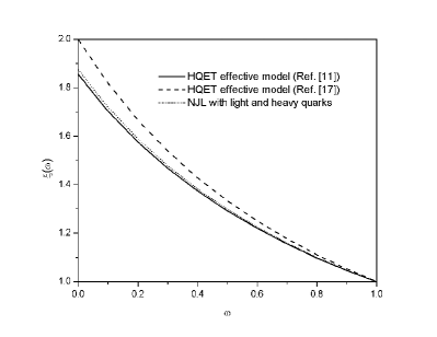
Figure 1: The Isgur-Wise function for the NJL model and other HQET effective models (Solid line - Ref. Ebert:1994tv , dashed line - Ref. Bardeen:1993ae (with $m=0$), dotted line - present approach.)

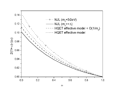
Figure 2: Effects of $\frac{1}{m_{0}}$ corrections to the Isgur-Wise function. The present results are represented by the solid ($m_{0}\rightarrow\infty$) and dotted with crosses ($m_{0}=5{\rm GeV}$) lines. The HQET effective model Ebert:1994tv results are represented by the dotted ($m_{0}\rightarrow\infty$) and dashed ($m_{0}=5{\rm GeV}$) lines.

In Fig. 1 we compare our result to that of Ebert et al. Ebert:1994tv . To see clearly the effect when comparing to , we choose the set of parameters to reproduce $f_{\pi}=93{\rm MeV}$, $m_{\pi}=140{\rm MeV}$, $m_{\rho}=770{\rm MeV}$ and $M_{B}=5.3{\rm GeV}$, obtaining $m_{u}=m_{d}=300{\rm MeV}$, $\Lambda=875{\rm MeV}$, $m_{s}=510{\rm MeV}$, $m_{B}=5.1{\rm GeV}$ and $G=2.9{\rm GeV^{-2}}$. In contrast with Ebert:1994tv , no independent coupling for the heavy meson sector needs to be inserted on the model in order to reproduce the light-light and heavy-light mesons masses, although a very low $B$ meson weak decay constant is obtained ($f_{B}=59{\rm MeV}$). Nevertheless, other processes that could be important to the correct description of this decay constant, as mesons loops, are absent in the present treatment. In the same figure, we also compare to the HQET effective model presented in Bardeen:1993ae where

$$\xi(\omega)=\frac{2}{1+\omega}.$$ (9)

in both $m_{0}\rightarrow\infty$ and $m\rightarrow 0$ limits. As we see, differences become more significant as $\omega$ goes to zero. The results obtained from the present model are very close to the results obtained in Ebert:1994tv . The differences of both models to the results presented on Bardeen:1993ae are due to finite light constituent quark mass effects: even in the $m_{0}\rightarrow\infty$ limit, result (9) is only achieved when $m=0$.

In Fig. 2 we present the comparison between the behaviour of the Isgur-Wise function as $m_{0}$ goes from $5{\rm GeV}$ to $50{\rm GeV}$ ($m_{0}\gg\Lambda$), computed on both present and Ebert:1994tv models (corrections of order $1/m_{0}$ on the HQET effective model of Ref. Ebert:1994tv were included). As can be viewed from Fig. 2, as $m_{0}$ increases the slope of the Isgur-Wise function on the present model increases, while the same slope decreases on the model presented on Ebert:1994tv . The magnitude of the changes on the slope of the Isgur-Wise function is also different in the two models.

Finally, let us mention that a derivative expansion of the bosonized version of the model can be employed to construct an effective mesonic Lagrangian, as was done for the light quark sector Ebert:1985kz . One problem is that such an expansion assumes small momenta for the corresponding meson bosonized fields, while for heavy mesons they are large. It is possible, however, to overcome this problem in a way that the treatment of light and heavy mesons is as symmetric as possible, so that at any stage the heavy pseudoscalars would become Goldstone bosons if the quarks were light. Further details will be further elaborated elsewhere inpreparation .

References

- (1) J. Gasser and H. Leutwyler, Annals Phys. 158 (1984) 142.
- (2) J. F. Donoghue, E. Golowich and B. R. Holstein, Camb. Monogr. Part. Phys. Nucl. Phys. Cosmol. 2 (1992) 1.
- (3) H. Georgi, Phys. Lett. B240, 447 (1990).
- (4) M. Neubert, Phys. Rept. 245, 259 (1994).
- (5) A. V. Manohar and M. B. Wise, Camb. Monogr. Part. Phys. Nucl. Phys. Cosmol. 10, 1 (2000).
- (6) U. Vogl and W. Weise, Prog. Part. Nucl. Phys. 27, 195 (1991).
- (7) S. P. Klevansky, Rev. Mod. Phys. 64, 649 (1992).
- (8) T. Hatsuda and T. Kunihiro, Phys. Rept. 247, 221 (1994).
- (9) R. Alkofer, H. Reinhardt, and H. Weigel, Phys. Rept. 265, 139 (1996).
- (10) C. V. Christov et al., Prog. Part. Nucl. Phys. 37, 91 (1996).
- (11) D. Ebert, T. Feldmann, R. Friedrich, and H. Reinhardt, Nucl. Phys. B434, 619 (1995).
- (12) A. Deandrea, N. Di Bartolomeo, R. Gatto, G. Nardulli, and A. D. Polosa, Phys. Rev. D58, 034004 (1998).
- (13) A. Hiorth and J. O. Eeg, Phys. Rev. D66, 074001 (2002).
- (14) W. A. Bardeen, E. J. Eichten, and C. T. Hill, Phys. Rev. D68, 054024 (2003).
- (15) C.-S. Huang, C. Liu, and C.-T. Yan, Phys. Rev. D62, 054019 (2000).
- (16) C. Schuren, E. Ruiz Arriola, and K. Goeke, Nucl. Phys. A547, 612 (1992).
- (17) W. A. Bardeen and C. T. Hill, Phys. Rev. D49, 409 (1994).
- (18) E. Ruiz Arriola, Acta Phys. Polon. B 33, 4443 (2002)
- (19) D. Ebert and H. Reinhardt, Nucl. Phys. B271, 188 (1986).
- (20) N. Isgur and M.B. Wise, Phys. Lett. B232, 113 (1989).
- (21) A. L. Mota and E. Ruiz Arriola (work in preparation)