New interpretation of matter-antimatter asymmetry based on branes and possible observational consequences

Rong-Gen Cai¹, Tong Li², Xue-Qian Li² and Xun Wang²

1. Institute of Theoretical physics, Chinese Academy of Sciences, Beijing 100080

2. Department of Physics, Nankai University, Tianjin 300071

I Introduction

One of the major tasks of the modern particle-cosmology is to explore a reasonable interpretation of the observed matter-antimatter asymmetry in our universeantimatter . The widely acceptable picture is that there must exist three key factors, namely, the CP violationCP1 , baryon number non-invariance and existence of a stage out of equilibrium. However, in the Standard Model (SM), the CP violation induced by the non-zero CKM CP phase is not large enough to meet the requirementCP2 . Therefore, either there is new physics beyond SM which can cause larger CP violationCP3 , or exist other mechanisms or picture which result in the observational matter asymmetry.

One alternative interpretation was proposed that the antimatter was repelled to other corners of the universe and in our part of the universe, only matter resides. Thus definitely, the antimatter would fly to our part and there is a possibility to be observed before it annihilates with the regular matter particles. The Alpha-Magnetic-Spectrometer project is set to observe the anti-helium fluxAMS1 ; AMS2 ; AMS . On the theoretical aspect, some authors have discussed existence of antimatter regions and possible flux to our detectorKhlopov . They consider large domains in the universe generated due to inflation, which then convert into antimatter regions. The evolution of the antimatter regions may result in an anti-star globular cluster. It is interesting to note that the CP may be violated spontaneouslyT.D.Lee ; Weinberg . In ref. Khlopov , the authors also suggest that separation of matter and antimatter is caused by such spontaneous CP violation.

In this work, we propose another possible picture based on the brane physics. Suppose that after the Big Bang or inflation epoch, CP symmetry is spontaneously broken and the two branes correspond to different ground states of matter and antimatter respectively. By the end of this phase transition, matter and antimatter begun to reside on different branes. Following Goldberger and Wise Wise , we introduce a complex scalar fields which is responsible for the spontaneous CP symmetry breaking. That is a scalar field which only applies to the extra dimension and is different from that in the standard model in our four-dimension spacetime. The vacuum expectation values (VEV) may be CP-phase dependent, so that the two branes correspond to different VEV’s and then accommodate matter and antimatter respectively.

According to the general theory of the brane physics, the gauge fields are confined on each brane, but only the gravitational field can extend to the extra dimension(s). The matter and antimatter attract each other via gravitational force. To oppose the gravitational attraction which may lead to a collision of the two branes to destroy the universe, the scalar field can cause a Casimir effect. The Casimir effect which can be calculated in the qunatum field theory, results in a repulsive force against the gravitational attraction. We find that the repulsive force caused by the Casimir effect is much stronger than the gravitational force as long as the separation of the two branes is small. Thus it may cause a cosmological consequence, that at the early epoch after the Big Bang, the two branes were closer, but they have been repelled from each other and the trend would continue till some day the two branes are sufficiently separated and then the gravitational force observed in our four-dimensional spacetime would obviously deviate from the Newton’s universal gravitational law. The picture seems to cause an unstable system. In the work Wise , the authors also suggested existence of a scalar field which has different vacuum expectation values at two branes (in their work, the other brane is empty) and a positive potential which leads to a repulsive force between the two branes is resulted in. The force can balance the gravitational force between the branes as it is applied to our picture, but it depends on the difference of the expectation values on the two branes. The Casimir repulsive force is an alternative possibility.

Moreover, we suppose that there is a potential barrier at the boundary of each brane which is similar to the surface tension for a water membrane. The barrier prevents the matter or antimatter to enter the space between the two branes and jump from one brane to another. In this work, we describe the barrier by a delta function, i.e.

$$V(\xi)=a\delta(\xi)+a\delta(\xi-\pi r_{c}),$$

where $a$ is a dimensionless parameter to be determined and $\pi r_{c}$ is the separation between the two branes at present.

The antimatter may traverse across the gap between the two branes via the quantum tunnelling. Thus an antimatter flux which has already come in our universe, may freely propagate in our brane, i.e. our matter world, until it annihilates with regular matter. Since the matter density in our universe is dilute, as the first order of approximation, we ignore its possible annihilation with matter before the flux reaches our detector. Thus the AMS may detect such antimatter flux and the measurement can provide us some detailed information about the antimatter world. As suggested, the AMS measures the flux of anti-helium from the antimatter world. It is reasonable to suppose that the abundance of anti-helium in the anti-matter world is the same as that of helium in our matter-world, and then we can estimate its flux.

We study the detection possibility in the naive flat-spacetime model and the Randall-Sundrum model whose metric tensor is suggested by the authors of RS . In the Randall-Sundrum model the ”compactification radius” between two branes $r_{c}$ is determined by solving the eletroweak hierarchy problem. Instead, we let $r_{c}$ be a free parameters which must be much smaller than 1 mm for the observation of gravitational law and numerically evaluate the flux of antimatter in our universe. However, we will show that in the future universe the two branes will be repelled away from each other by the Casimir force and finally the gravitational balances the Casimir force and then $r_{c}$ would reach its maximum and the observational Newton’s law will be obviously different from the present form. Indeed, we do not expect to predict very accurate value for the antimatter flux, but gain important information about such flux while the future AMS experiment will help to fix concerned parameters.

After this introduction, we formulate the Casimir effect of the scalar field and discuss its consequence. Then we derive the Schrödinger equation for the fifth dimension in the non-relativistic approximation and in the next section, we evaluate the antimatter flux which penetrates the potential barriers to reach our AMS detector. By the astronomical data we roughly estimate the antimatter flux which can be captured by the AMS detector. In the last section, we make more discussions and draw our conclusion.

II Interaction between the two branes

II.1 The gravitational attraction between the two branes

Different from the regular brane scenario where one brane is empty and the normal matter resides on another, both branes are occupied by massive particles and as the gravitational force line can cross the fifth dimension, the two branes attract each other. Thus, let us first estimate the gravitational attraction between the branes.

Considering a three-dimensional area $S$ on the brane where matter uniformly distributes, the gravitational filed strength $E$ can be derived in terms of the Gauss’ law in four-dimension. The mass density of the matter in our universe (anti-matter in the anti-world) is $\rho$.

By the Gauss’ law, we have

$${2\over G_{5}}ES = \rho S$$

$$E = {G_{5}\rho\over 2},$$ (1)

where $G_{5}$ is the five-dimensional gravitational constant, whose relation with four-dimensional gravitational constant $G_{4}$ is basically $G_{5}=2r_{c}G_{4}$G45_1 ; G45_2 .

Thus the gravitational force density between the two branes reads as

$$f = E\rho=G_{4}r_{c}\rho^{2}.$$ (2)

II.2 A possible Casimir force

To balance the gravitational force between two branes, following the literature, it is supposed that a scalar field exists between the two branes and due to its existence there is a Casimir effect. Under the periodic boundary condition, the Casimir energy density induced by a massless scalar field is given asCasimir1 ; Casimir2

$$V^{P} = {1\over 2}\sum^{\infty}_{n=-\infty}\int{d^{4}k\over(2\pi)^{4}}\text{ln}(k^{2}+{n^{2}\over r_{c}^{2}})$$ (3)

$$= -{1\over 2}{\partial\over\partial s}|_{s=0}\left[\sum^{\infty}_{n=-\infty}\int{d^{4}k\over(2\pi)^{4}}(k^{2}+{n^{2}\over r_{c}^{2}})^{-s}\right]$$

$$= -{1\over 2}{\partial\over\partial s}|_{s=0}\left[\sum^{\infty}_{n=-\infty}\int{d^{4}k\over(2\pi)^{4}}{1\over\Gamma(s)}\int^{\infty}_{0}dte^{-(k^{2}+{n^{2}\over r_{c}^{2}})t}t^{s-1}\right]$$

$$= -{\partial\over\partial s}|_{s=0}\left[{\pi^{2}\over(2\pi)^{4}r_{c}^{4}}{\Gamma(s-2)\over\Gamma(s)}(r_{c})^{2s}\zeta(2s-4)\right]$$

$$= -{\pi^{2}\over(2\pi)^{4}r_{c}^{4}}\zeta^{\prime}(-4)$$

$$= -{\pi^{2}\over(2\pi)^{4}r_{c}^{4}}{3\over 4\pi^{4}}\zeta(5)$$

$$\simeq -{3.102\over 64\pi^{6}r_{c}^{4}},$$

where $\zeta(5)\simeq 1.034$.

The Casimir force density is

$$F^{P} = -{\partial\over\partial r_{c}}V^{P}$$ (4)

$$= -{12.408\over 64\pi^{6}r_{c}^{5}}.$$

That is an attractive force density and cannot play a role to oppose the gravitational force. By contraries, if the boundary condition is anti-periodic, one has the Casimir energy density as

$$V^{A} = -{15\over 16}V^{P}$$ (5)

$$= {3.102\over 64\pi^{6}r_{c}^{4}}{15\over 16},$$

and a repulsive Casimir force density

$$F^{A} = {46.53\over 256\pi^{6}r_{c}^{5}}$$ (6)

is resulted in.

By the data, one can notice that for a small separation between the two branes, i.e. the distance must be smaller than 1 mm requested by the observation of gravitational law, the repulsive Casimir force is larger than the attractive force between the two branes. One can conjecture that at the early epoch of the universe, the two branes were close to each other, and just due to the repulsive force, the two branes gradually are repelled away from each other and will continue to be separated further till one typical distance which is about $10^{5}$ m, the Casimir force would balance the gravitational force and then the observational gravitational law definitely deviates from the Newton’s law, and becomesG45_2

$$V_{4}=-{G_{4}M\over r}(1+(n+1)e^{-\sqrt{n}r/R}),$$ (7)

where $G_{4}$ is the four-dimension universal gravitational constant, $n$ is the number of extra dimensions and $R$ is a typical distance in the extra dimension.

The authors of Ref. Wise introduced an extra scalar field and an interaction on the two branes in the Randall-Sundrum scenario. The interaction of the scalar field between two branes yields an effective four-dimensional potential for $r_{c}$. Then the potential can help to stabilize $r_{c}$. The repulsive force caused by the Casimir effects is another possibility.

III Transition rates of the anti-matter flux

To obtain the transition rate of the anti-matter, one needs to establish a Schrödinger equation along the fifth dimension. The form of the five-dimension Schrödinger equation depends on the metric for any concerned brane model. Below, we choose two models, namely the naive flat space-time and R-S(Randall-Sundrum)RS metrics which are intensively discussed in literature as examples to demonstrate how to evaluate the anti-matter flux which would be observed by the AMS.

III.1 Naive flat space-time

We first discuss the simplest model, the naive flat space-time. The metric for naive flat five-dimensional space-time is given as

$$ds^{2}=\eta_{\mu\nu}dx^{\mu}dx^{\nu}+d\xi^{2},$$ (8)

where $\eta_{\mu\nu}$ is the metric for a four-dimensional Minkowski spacetime. Substituting the metric into the five-dimensional Klein-Gordon equation, one has

$$-({\partial\over\partial t})^{2}\Psi+({\partial\over\partial\vec{x}})^{2}\Psi+({\partial\over\partial\xi})^{2}\Psi-m^{2}\Psi = 0.$$ (9)

Decomposing the wavefunction $\psi$ into a product form

$$\Psi = e^{i\vec{k}\cdot\vec{x}}\psi(\xi,t),$$ (10)

and substituting it into eq.(9), one can eventually obtain an equation which only contains differentiation of $\psi$ with respect to the fifth dimension variable $\xi$ and time $t$,

$$\left[({\partial\over\partial\xi})^{2}-({\partial\over\partial t})^{2}-(m^{2}+\vec{k}^{2})\right]\psi(\xi,t) = 0$$ (11)

It is noted that we ignore the regular interactions among the particles on the branes. Then taking the non-relativistic approximation,

$$\psi(\xi,t) = \varphi(\xi,t)e^{-imt}$$

$$-({\partial\over\partial t})^{2}\psi \simeq \left[2im{\partial\varphi\over\partial t}+m^{2}\varphi\right]e^{-imt}$$ (12)

and substituting it into eq.(11), we get

$$2mi{\partial\varphi\over\partial t}+({\partial\over\partial\xi})^{2}\varphi+\left(-\vec{k}^{2}\right)\varphi = 0,$$ (13)

namely, it is

$$-{1\over 2m}({\partial\over\partial\xi})^{2}\varphi+\left({\vec{k}^{2}\over 2m}\right)\varphi = E\varphi.$$ (14)

After introducing two $\delta$ potentials at the surfaces of the two branes and through a simple manipulation one has the Schrödinger equation along the fifth dimension with an effective potential and corresponding boundary conditions as

$$-{1\over 2m}({\partial\over\partial\xi})^{2}\varphi+\left({\vec{k}^{2}\over 2m}+a\delta(\xi)+a\delta(\xi-\pi r_{c})\right)\varphi = E\varphi.$$ (15)

At the anti-world brane, the solution of eq.(15) is:

$$\varphi(\xi) = e^{i\alpha\xi}+R_{1}e^{-i\alpha\xi}\;\;\;\;\;\;\;\;\;\;\xi<0,$$

$$\varphi(\xi) = S_{1}e^{i\alpha\xi}+R_{2}e^{-i\alpha\xi}\;\;\;\;\;\;\xi>0.$$ (16)

At our brane, the solution of eq.(15) is:

$$\varphi(\xi) = S_{1}e^{i\alpha\xi}+R_{2}e^{-i\alpha\xi}\;\;\;\;\;\;\xi<\pi r_{c},$$

$$\varphi(\xi) = S_{2}e^{i\alpha\xi}\;\;\;\;\;\;\;\;\;\;\;\;\;\;\;\;\;\;\;\;\;\;\;\xi>\pi r_{c}.$$ (17)

where $\alpha$ is an eigenvalue for eq.(14) as $\alpha=\sqrt{2mE-\vec{k}^{2}}$.

The boundary conditions on the brane surfaces at $\xi=0$ and $\xi=\pi r_{c}$ respectively demand

$$\left(\varphi^{\prime}(0^{+})-\varphi^{\prime}(0^{-})\right) = 2ma\varphi(0),$$

$$\left(\varphi^{\prime}((\pi r_{c})^{+})-\varphi^{\prime}((\pi r_{c})^{-})\right) = 2ma\varphi(\pi r_{c}),$$ (18)

we can find the barrier penetration rate $T=|S_{2}|^{2}$ as

$$T = |S_{2}|^{2}={(2\alpha)^{2}\over\left(4am+{2a^{2}m^{2}\sin(2\alpha\pi r_{c})\over\alpha}\right)^{2}+\left(2\alpha+{2a^{2}m^{2}(\cos(2\alpha\pi r_{c})-1)\over\alpha}\right)^{2}}.$$ (19)

III.2 The RS model

In the RS model, the corresponding metric is

$$ds^{2} = e^{2\phi(\xi)}\eta_{\mu\nu}dx^{\mu}dx^{\nu}+d\xi^{2}$$

$$\phi(\xi) = -\kappa\xi$$ (20)

where $0\leq\xi\leq\pi r_{c}$ is the coordinate for an extra dimension and $r_{c}$ is the ”compactification radius” of the extra dimension RS . The Klein-Gorden equation reads

$${1\over\sqrt{-g}}\partial_{A}(\sqrt{-g}g^{AB}\partial_{B}\Psi)-m^{2}\Psi = 0.$$ (21)

Substituting the metric into the field equation, one has

$$-4\kappa{\partial\Psi\over\partial\xi}-e^{2\kappa\xi}({\partial\over\partial t})^{2}\Psi+e^{2\kappa\xi}({\partial\over\partial\vec{x}})^{2}\Psi+({\partial\over\partial\xi})^{2}\Psi-m^{2}\Psi = 0.$$ (22)

Similar to the flat space-time case, decomposing the wavefunction $\psi$ into a product form

$$\Psi = e^{i\vec{k}\cdot\vec{x}}e^{-2\phi(\xi)}\psi(\xi,t),$$ (23)

and substituting it into eq.(22), we eventually obtain the equation which only contains differentiation of $\psi$ with respect to the fifth dimension $\xi$ and time $t$,

$$\left[({\partial\over\partial\xi})^{2}-e^{2\kappa\xi}({\partial\over\partial t})^{2}-(4\kappa^{2}+m^{2}+\vec{k}^{2}e^{2\kappa\xi})\right]\psi(\xi,t) = 0.$$ (24)

Then with the non-relativistic approximation,

$$\psi(\xi,t) = \varphi(\xi,t)e^{-imt}$$

$$-({\partial\over\partial t})^{2}\psi \simeq \left[2im{\partial\varphi\over\partial t}+m^{2}\varphi\right]e^{-imt}$$ (25)

we get

$$2me^{2\kappa\xi}i{\partial\varphi\over\partial t}+({\partial\over\partial\xi})^{2}\varphi+\left(e^{2\kappa\xi}m^{2}-4\kappa^{2}-m^{2}-\vec{k}^{2}e^{2\kappa\xi}\right)\varphi = 0.$$ (26)

Further, we can rewrite the above equation as

$$({\partial\over\partial\xi})^{2}\varphi = \left[(\vec{k}^{2}-m^{2}-2mE)e^{2\kappa\xi}+m^{2}+4\kappa^{2}\right]\varphi.$$ (27)

Considering two $\delta$ barriers at the two brane surfaces, we finally arrive at what we want to have

$$-{1\over 2m}({\partial\over\partial\xi})^{2}\varphi+\left[{1\over 2m}(\vec{k}^{2}-m^{2})e^{2\kappa\xi}+{1\over 2m}(m^{2}+4\kappa^{2})+a\delta(\xi)+a\delta(\xi-\pi r_{c})\right]\varphi = Ee^{2\kappa\xi}\varphi.$$ (28)

At the anti-world brane, the solution of eq.(28) is:

$$\varphi(\xi) = e^{i\alpha(\xi)}+R_{1}e^{-i\alpha(\xi)}\;\;\;\;\;\;\;\;\;\;\xi<0,$$

$$\varphi(\xi) = S_{1}e^{i\alpha(\xi)}+R_{2}e^{-i\alpha(\xi)}\;\;\;\;\;\;\xi>0,$$ (29)

and at our brane (matter), the solution of eq.(28) is:

$$\varphi(\xi) = S_{1}e^{i\alpha(\xi)}+R_{2}e^{-i\alpha(\xi)}\;\;\;\;\;\;\xi<\pi r_{c},$$

$$\varphi(\xi) = S_{2}e^{i\alpha(\xi)}\;\;\;\;\;\;\;\;\;\;\;\;\;\;\;\;\;\;\;\;\;\;\;\;\;\xi>\pi r_{c}.$$ (30)

where $\alpha(\xi)$ is the eigenvalue of eq.(27): $\alpha(\xi)={\sqrt{2mE+m^{2}-\vec{k}^{2}}\over\kappa}e^{\kappa\xi}$.

With the same boundary conditions which were depicted for the flat space-time case, we can find the barrier penetration rate $T=|S_{2}|^{2}$ as

$$T = |S_{2}|^{2}=1/\left\{\left[({ma\over\kappa})^{2}{1\over\beta_{1}\beta_{2}}(\cos(2(\beta_{2}-\beta_{1}))-1)+1\right]^{2}+\left[({ma\over\kappa})^{2}{1\over\beta_{1}\beta_{2}}\sin(2(\beta_{2}-\beta_{1}))+{ma\over\kappa}({1\over\beta_{1}}+{1\over\beta_{2}})\right]^{2}\right\},$$

$$\beta_{1} = {\sqrt{2mE+m^{2}-\vec{k}^{2}}\over\kappa},$$

$$\beta_{2} = {\sqrt{2mE+m^{2}-\vec{k}^{2}}\over\kappa}e^{\pi\kappa r_{c}}.$$ (31)

This expression of transition rate is different from that for the flat space-time case, some details would be manifested in the numerical results and the following figures.

III.3 The evolution of the two branes in RS model

The key point concerning the RS model is whether the evolution of the two-brane structure coincides with the present astronomical observation. To investigate the evolution, one needs to solve the five-dimensional Einstein’s equations for the ”compactification radius” $r_{c}$ at any timeEinstein . We rewrite the eq.(20) into a different form by assuming $\xi=r_{c}(t)\widetilde{\xi}$:

$$ds^{2} = (-e^{-2\kappa r_{c}(t)\widetilde{\xi}}+\widetilde{\xi}^{2}\dot{r_{c}}^{2})dt^{2}+e^{-2\kappa r_{c}(t)\widetilde{\xi}}d\vec{x}^{2}+r_{c}(t)^{2}d\widetilde{\xi}^{2}+2\widetilde{\xi}r_{c}(t)\dot{r_{c}}d\widetilde{\xi}dt$$ (32)

The five-dimensional Einstein’s equations are

$$G_{AB}\equiv R_{AB}-{1\over 2}Rg_{AB}=\widetilde{\kappa}^{2}T_{AB}$$ (33)

where $R_{AB}$ is the five-dimensional Ricci tensor, $R=g^{AB}R_{AB}$ the scalar curvature and the constant $\widetilde{\kappa}$ is related to the five-dimensional Newton’s constant with $\widetilde{\kappa}^{2}=8\pi G_{(5)}$Einstein1 . The right hand term $T_{AB}$ is the energy-momentum tensor.

Inserting the metric in eq.(32) into the Einstein equations, we can obtain the non-vanishing components of the Einstein tensor $G_{AB}$ which includes a derivative of $r_{c}$ with respect to time t. In principle, it is a self-consistent differential equation group and would be extremely difficult to solve, but with a reasonable approximation, one can be priori set the energy-momentum tensor for the bulk matter and the matter content on the branes, the differential equations can be solved. Then we would be able to obtain $r_{c}$ at any time. In practice, because the five-dimensional differential equations for $r_{c}(t)$ and the junction conditions are too complex, that even with the assumption, we are unable at present to get a solution, no matter analytical or numerical. In order to discuss the physics picture, let us take an extreme simplification. In eq. (A1) which is presented in the appendix, we assume that $\dot{r}_{c}$ is small, so that we can neglect the terms with higher powers of $\dot{r}_{c}$ and only keep $\dot{r}_{c}^{2}$ terms on the left-side of eq.(A1). The right-side of the energy tensor $T_{00}$ reflects a competition between the Casimir repulsion and gravitational attraction. As shown in previous subsection, at very early universe the Casimir repulsion dominates over the gravitational attraction between the matter on the two branes, $T_{00}$ is positive. If we can approximately set $T_{00}$ as a constant, the equation is simple and the solution is $r_{c}(t)\sim\exp(\alpha t)$ where $\alpha$ is a constant related to the $T_{00}$ and other parameters. It is an exponentially increasing function, namely the two branes would separate by the repulsive force. However, as shown above, $T_{00}$ is not a constant, and when $r_{c}$ reaches a certain value, the gravitational attraction becomes stronger, then the separation would slow down till completely stops when the two forces balance each other. Indeed, a complete solution for the evolution process is beyond the scope of the work and our present ability, we will pursue this topic in our future studies.

IV Numerical Result for phenomenology

Here for the numerical computations of the flux of antimatter to be detected at the AMS, we include all the necessary input parameters which are directly adopted from the concerned published literaturesRS ; data0 .

$$T = \bar{\rho}_{anti-helium}/\rho_{helium}$$ (34)

where $\bar{\rho}_{anti-helium}$ is the mass density of the anti-helium particles which overcome the brane barriers to transit into our brane, $m=m_{He}=4$ GeV, the dispersive velocity of helium is $v_{He}=1000$ km/s and $\kappa r_{c}=12$. The ”compactification radius” of the extra dimension $r_{c}$ and factor $a$ in the $\delta$ potential are regarded as free parameters.

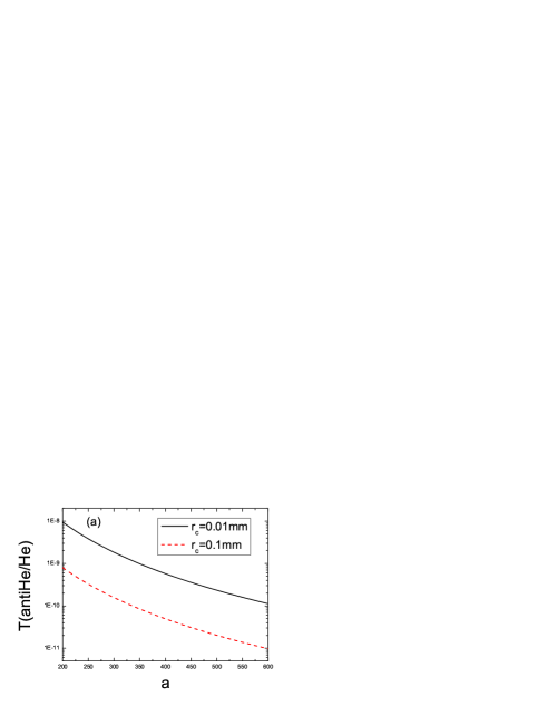
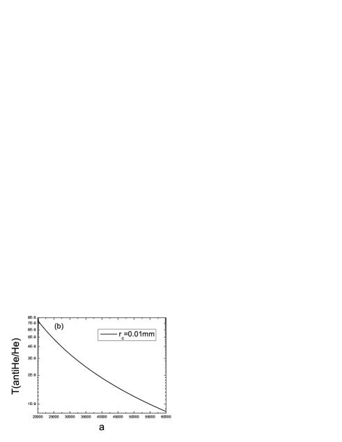
Figure 1: The anti-He/He flux-ratio (a) for the flat space-time model and (b) for the RS model.

In Fig. 1, we show the ratio of the anti-helium flux over helium flux in our three-dimension space, which can be detected by our detector on the earth or AMS. In this work, we are working on the naive flat spacetime and the RS-I model, the physics condition we set should determine a bound on $r_{c}$, while similar bounds may be gained by solving the hierarchy problemRS or the minimum condition of the effective potentialWise . Here we choose $r_{c}=0.01$ and 0.1 mm, which is consistent with present data on gravity. It is noted that the ratio drops very fast as the potential strength $a$ increases for the naive flat space-time model, but not so abruptly for the RS model. The flux ratio decreases very fast as the distance $r_{c}$ increases for the naive flat space-time model, but almost does not vary for the RS model. Let us roughly estimate the order of magnitude of the surface potential. It is of order $a/r_{c}\sim 2^{-8}a$ MeV, and as $a\sim 1000$, it is a few hundreds of eV. It seems reasonable.

The numbers of anti-helium particles which can be detected by the AMS should be

$$N={\Delta\Omega\over 4\pi}{\bar{\rho}_{anti-helium}\over m}|{\bf v}|\Delta S\Delta t\times f,$$ (35)

where the factor $\Delta\Omega/4\pi$ is from the random direction of the flux, $\bar{\rho}_{anti-helium}=\rho_{helium}\times T$ and $\rho_{helium}=23\%\rho_{b}$, $\rho_{b}=0.042\rho_{c}$, $\rho_{c}=1.87837\times 10^{-29}h^{2}$gcm^-3, $h=0.73$data0 , m is the mass of single helium particle, $|{\bf v}|=v_{He}$ is the average velocity of the anti-helium, $\Delta t$ is the duration of the detection which we take as one year, $\Delta S$ is the area of AMS with $\Delta\Omega\Delta S=0.65$ sr $m^{2}$AMS2 and $f$ is the detection efficiency of detecting such anti-helium particles by the AMS which we take as 100$\%$. In the dispersive , the authors decide that the average dispersion velocity of dark matter particles is within a range of 600 to 1000 km/s, and we just adopt the maximal value as a reasonable approximation for $v_{He}$. Obviously the theoretical prediction of $N$ depends on the model and the concerned parameters such as $r_{c}$ and $a$. Later, with a few typical parameter sets, we tabulate the number of anti-helium particles which may be detected by AMS in Fig. 2.

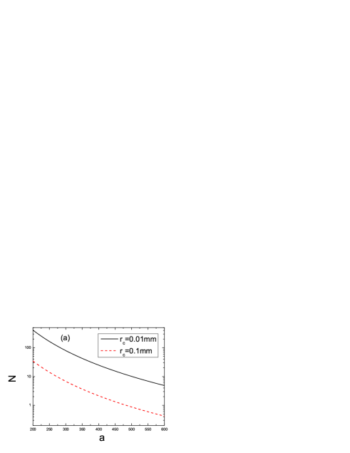
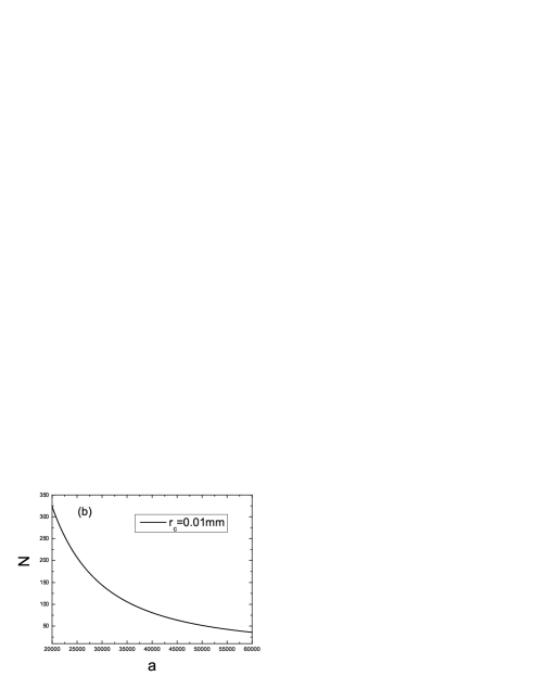
Figure 2: The number of anti-helium particles which can be detected by the AMS in one year (a) for the flat space-time model (b) for the RS model

Table 1: The number of anti-helium particles which can be detected by the AMS in one year for the flat space-time metric.

N	$a=200$	$a=250$	$a=300$	$a=350$	$a=400$	$a=450$	$a=500$	$a=550$	$a=600$
$r_{c}=0.01$ mm	$408$	$165$	$76$	$43$	$25$	$15$	$10$	$7$	$5$
$r_{c}=0.1$ mm	$34$	$14$	$7$	$4$	$2$	$1$	$0$	$0$	$0$

Table 2: The number of anti-helium particles which can be detected by the AMS in one year for the R-S metric.

N	$a=20000$	$a=25000$	$a=30000$	$a=35000$	$a=40000$	$a=45000$	$a=50000$	$a=55000$	$a=60000$
$r_{c}=0.01$ mm	$323$	$207$	$144$	$106$	$81$	$64$	$52$	$43$	$36$
$r_{c}=0.1$ mm	$323$	$207$	$144$	$106$	$81$	$64$	$52$	$43$	$36$

V Discussion and Conclusion

In this work we propose a possible physical picture to interpret the matter-antimatter asymmetry observed in our universe. We suppose that at the early epoch of the universe evolution, maybe after the inflation stage, the CP symmetry is spontaneously broken, and the two branes correspond to the two ground states of CP. Thus the matter and antimatter were separated onto two different branes. A complex scalar field which only applies to the extra dimension, is introduced to be responsible for the spontaneous CP symmetry breaking and the CP phase-dependent vacuum expectation values can be different at the two branes. The scalar field existing between the two branes, causes a Casimir force which repels the two branes away from each other. The two branes would attract each other via gravitational force. Preventing the two branes to collide and matter-antimatter annihilate, the scalar field which obeys anti-periodic boundary conditions on the two branes provides a repulsive force to opposes the gravitational attraction. For smaller distance between two branes, as shown in the text, the Casimir repulsive force is stronger than the gravitational attraction and the consequence is that the two branes would be pushed away from each other till sometime which would be much later than today, the two forces are balanced and an equilibrium is reached (roughly, the separation would be a few hundreds of km). With extra dimensions, the $1/r^{2}$ Newton’s gravitational law must be modified G45_1 ; G45_2 as shown in the form of eq. (7). Since today one does not observe any deviation from the $1/r^{2}$ law at the macroscopic scale, he must consider that $r_{c}$ is sufficiently small, such as less than 0.1 mm. In this work, we take $r_{c}=0.1$ and 0.01 mm, of course it is only an illustration. In many, many years, when the two branes are separated very far by meters, the observational gravitation law will deviate from $1/r^{2}$ form. If one needs to find the evolution of the brane world, namely how the two branes are separated from initial $r_{c}\approx 0$ to the present value, he must solve the 5-dimensional time-dependent Einstein equation, but it is beyond the scope of the present work and we will not discuss the evolution process here.

As discussed by many authors, generally the matter (antimatter) and gauge bosons are forbidden to enter the fifth dimension except the gravitational force lines, to realize the picture, we suggest that there is a barrier on the edge of the brane in analog to the surface tension of water membrane. We use a simple delta function to describe the barrier. Like the picture for Hawking radiation of black holes, the quantum effects may cause a quantum tunnelling of the matter and antimatter from one brane to another.

The antimatter which reside on another brane would have a probability to transit into our brane with matter only. The flux depends on the barrier strength and may be detected by the detector on earth. The AMS would be an ideal apparatus to do the job. According to the preliminary results of AMS on the antimatter fluxAMS , we can estimate the brane-barrier strength. In this work, we consider two popular models, the naive flat space-time model and the R-S models, to carry out the calculations. We find that their results about antimatter flux are quite different as shown in Fig. 1.

This picture is indeed somehow ad hoc and speculative, but provides a possible interpretation for the matter-antimatter asymmetry observed in our universe, and suggests an existence of the antimatter flux which can be detected by AMS. There are indeed a few adjustable parameters in the picture which cannot be determined from the first principle so far and need to be fixed by the measurements of AMS. We are eagerly waiting for the measurement results of AMS because they may tell us much more information about the universe and also probe our proposal.

Acknowledgement:

We benefit greatly from very stimulating and active discussions with Xiao-Gang He, indeed some initiative ideas are produced during such conversations. We also thank H.S. Chen for helpful discussions and introduction about new progress on the AMS project. Discussion with Liu Zhao is also helpful and fruitful. This work is partly supported by the National Natural Science Foundation of China (NNSFC), No.10475042.

Appendix: The five-dimensional Einstein equations including derivative with respect to time

$$3\kappa(9\widetilde{\xi}^{5}\dot{r_{c}}^{6}-3\kappa\dot{r_{c}}^{6}r_{c}\widetilde{\xi}^{6}+2\kappa r_{c}e^{-6\kappa r_{c}\widetilde{\xi}}+e^{-4\kappa r_{c}\widetilde{\xi}}\widetilde{\xi}\dot{r_{c}}^{2}+4e^{-2\kappa r_{c}\widetilde{\xi}}\widetilde{\xi}^{3}r_{c}\ddot{r_{c}}\dot{r_{c}}^{2}+9\widetilde{\xi}^{2}\dot{r_{c}}^{2}r_{c}\kappa e^{-4\kappa r_{c}\widetilde{\xi}}+4\widetilde{\xi}^{4}\dot{r_{c}}^{4}r_{c}\kappa e^{-2\kappa r_{c}\widetilde{\xi}}$$

$$-2\widetilde{\xi}^{3}\dot{r_{c}}^{4}e^{-2\kappa r_{c}\widetilde{\xi}})/(r_{c}(e^{-2\kappa r_{c}\widetilde{\xi}}+3\widetilde{\xi}^{2}\dot{r_{c}}^{2})^{2})=\widetilde{\kappa}^{2}T_{00},\hskip 85.35826pt(\text{A}1)$$

$$-e^{-2\kappa r_{c}\widetilde{\xi}}(-2e^{-2\kappa r_{c}\widetilde{\xi}}\kappa r_{c}^{2}\widetilde{\xi}\ddot{r_{c}}+29e^{-2\kappa r_{c}\widetilde{\xi}}\kappa^{2}r_{c}^{2}\widetilde{\xi}^{2}\dot{r_{c}}^{2}+18\widetilde{\xi}^{4}\dot{r_{c}}^{4}\kappa^{2}r_{c}^{2}-12\widetilde{\xi}^{3}\dot{r_{c}}^{4}\kappa r_{c}+6\kappa^{2}r_{c}^{2}e^{-4\kappa r_{c}\widetilde{\xi}}+e^{-2\kappa r_{c}\widetilde{\xi}}r_{c}\ddot{r_{c}}$$

$$+e^{-2\kappa r_{c}\widetilde{\xi}}\dot{r_{c}}^{2}+5\kappa\dot{r_{c}}^{2}\kappa e^{-2\kappa r_{c}\widetilde{\xi}}r_{c})/(r_{c}^{2}(e^{-2\kappa r_{c}\widetilde{\xi}}+3\widetilde{\xi}^{2}\dot{r_{c}}^{2})^{2})$$

$$=\widetilde{\kappa}^{2}T_{11}=\widetilde{\kappa}^{2}T_{22}=\widetilde{\kappa}^{2}T_{33},\hskip 199.16928pt(\text{A}2)$$

$$-3\kappa r_{c}(2e^{-4\kappa r_{c}\widetilde{\xi}}\kappa r_{c}+8e^{-2\kappa r_{c}\widetilde{\xi}}\kappa r_{c}\widetilde{\xi}^{2}\dot{r_{c}}^{2}-\widetilde{\xi}\dot{r_{c}}^{2}e^{-2\kappa r_{c}\widetilde{\xi}}+3\widetilde{\xi}^{4}\dot{r_{c}}^{4}\kappa r_{c}-9\widetilde{\xi}^{3}\dot{r_{c}}^{4}-e^{-2\kappa r_{c}\widetilde{\xi}}\widetilde{\xi}r_{c}\ddot{r_{c}})/(e^{-2\kappa r_{c}\widetilde{\xi}}+3\widetilde{\xi}^{2}\dot{r_{c}}^{2})^{2}$$

$$=\widetilde{\kappa}^{2}T_{44},\hskip 284.52756pt(\text{A}3)$$

$$-3\dot{r_{c}}\widetilde{\xi}\kappa(e^{-2\kappa r_{c}\widetilde{\xi}}\widetilde{\xi}\dot{r_{c}}^{2}-9\widetilde{\xi}^{3}\dot{r_{c}}^{4}+4\kappa r_{c}e^{-4\kappa r_{c}\widetilde{\xi}}+19\widetilde{\xi}^{2}\dot{r_{c}}^{2}r_{c}\kappa e^{-2\kappa r_{c}\widetilde{\xi}}+15\kappa\dot{r_{c}}^{4}r_{c}\widetilde{\xi}^{4}-2e^{-2\kappa r_{c}\widetilde{\xi}}\widetilde{\xi}r_{c}\ddot{r_{c}})/(e^{-2\kappa r_{c}\widetilde{\xi}}+3\widetilde{\xi}^{2}\dot{r_{c}}^{2})^{2}$$

$$=0,\hskip 312.9803pt(\text{A}4)$$

where $T_{00},T_{11},T_{22},T_{33},T_{44}$ are the components of energy-momentum tensor $T_{AB}$ of the bulk matter and the matter content in the brane, which expressions can be found in Ref.Einstein1 .

References

- (1) M. Dine, A. Kusenko, Rev. Mod. Phys. 76 (2004) 1; W. Buchmuller, P. Di Bari, M. Plumacher, Nucl. Phys. B643 (2002) 367; A. G. Cohen, A. De Rujula, S. L. Glashow, Astrophys. J. 495 (1998) 539.
- (2) M. Kobayashi and T. Maskawa, Prog. Theor. Phys. 49 (1973) 652; N. Cabibbo, Phys. Rev. Lett. 10 (1963) 531.
- (3) A. J. Buras and M. K. Harlander, A Top Quark Story: Quark Mixing, CP Violation and Rare Decays in the Standard Model, in Heavy Flavours, ed. A. J. Buras and M. Lindner, Advanced Series on Directions in High Energy Physics (World Scientific, Singapore, 1992), Vol. 10, p. 58.
- (4) L. Wolfenstein, Phys. Rev. Lett. 13 (1964) 562; H. Sonoda, Nucl. Phys. B326 (1989) 135; J. Ellis et al., CERN-TH-6755-92 (1992).
- (5) AMS Collaboration, A. Barrau et al., astro-ph/0103493.
- (6) AMS Collaboration, J. Alcaraz et al., Nucl. Instrum. Meth. A478 (2002) 119-122.
- (7) AMS Collaboration, B. Borgia et al., IEEE Trans. Nucl. Sci. 52 (2005) 2786-2792.
- (8) V. M. Chechetkin, M. G. Sapozhnikov, M. Yu. Khlopov and Ya. B. Zeldovich, Phys. Lett. B118 (1982) 359; K. M. Belotsky, Yu. A. Golubkov, M. Yu. Khlopov, R. V. Konoplich and A. S. Sakharov, Yadernaya Fizika 63 (2000) 290; A. S. Sakharov, M. Yu. Khlopov and S. G. Rubin, Talk given at the CAPP2000 Conference on Cosmology and Particle Physics 17-28 July 2000, Verbier, Switzerland, Cosmology and Particle Physics, AIP Conference Proceedings 555 (2001) 421; M. Yu. Khlopov, S. G. Rubin and A. S. Sakharov, Talk given at 14th Rencontres de Blois: Matter - Anti-matter Asymmetry, Chateau de Blois, France, 17-22 Jun 2002, hep-ph/0210012.
- (9) T.D. Lee, Phys. Rev. D8 (1973) 1226.
- (10) S. Weinberg, Phys. Rev. Lett. 37 (1976) 657.
- (11) W. D. Goldberger and M. B. Wise, Phys. Rev. Lett. 83 (1999) 4922.
- (12) L. Randall and R. Sundrum, Phys. Rev. Lett. 83 (1999) 3370; L. Randall and R. Sundrum, Phys. Rev. Lett. 83 (1999) 4690.
- (13) E.G. Floratos and G. L. Leotaris, Phys. Lett. B465 (1999) 95.
- (14) A. Kehagias and C. Sfetsos, Phys. Lett. B472 (2000) 39.
- (15) E. Ponton and E. Poppitz, JHEP 0106 (2001) 019.
- (16) M. Ito, Nucl. Phys. B668 (2003) 322.
- (17) P. Binétruy, C. Deffayet and D. Langlois, Nucl. Phys. B615 (2001) 219; D. Langlois and L. Sorbo, Phys. Lett. B543 (2002) 155.
- (18) P. Binétruy, C. Deffayet, U. Ellwanger and D. Langlois, Phys. Lett. B477 (2000) 285.
- (19) W.-M. Yao, et al., Particle Data Group, J. Phys. G33 (2006) 1.
- (20) R. Cowsik, C. Ratnam and P. Bhattacharjee, Phys. Rev. Lett. 76 (1996) 3886.