RS model with a small curvature and gravity effects in $\mathbf{e^{+}e^{-}}$ annihilation into leptons at the LC

Abstract

The Randall-Sundrum (RS) model with a small curvature is considered. The mass spectrum of Kaluza-Klein (KK) gravitons in such a scheme is similar (although not equivalent) to that in a model with one extra dimension in a flat metric. The gravity effects in the processes $e^{+}e^{-}\rightarrow e^{+}e^{-}$ and $e^{+}e^{-}\rightarrow\mu^{+}\mu^{-}$ at the collision energy 1 TeV are presented. Our calculations are based on the previously obtained formula for virtual graviton contributions which takes into account both a discrete character of the mass spectrum and nonzero widths of the KK gravitons.

1 Randall-Sundrum model with the small curvature

The Randall-Sundrum (RS) model [1] is one realization of extra dimension (ED) theories in a slice of the AdS₅ space-time with the following background warped metric:

$$ds^{2}=e^{2\kappa(\pi r-|y|)}\,\eta_{\mu\nu}\,dx^{\mu}\,dx^{\nu}+dy^{2}\;,$$ (1)

where $y=r\theta$ ($-\pi\leqslant\theta\leqslant\pi$), $r$ being the “radius” of extra dimension, and $\eta_{\mu\nu}$ is the Minkowski metric. The points $(x_{\mu},y)$ and $(x_{\mu},-y)$ are identified, so we work on the orbifold $S^{1}/\mathbf{Z_{2}}$.

The parameter $\kappa$ defines a 5-dimensional scalar curvature of the AdS₅ space. Namely, the Ricci curvature invariant for this AdS₅ space, $\mathcal{R}^{(5)}$, is given by $\mathcal{R}^{(5)}=-20\,\kappa^{2}$. For the sake of simplicity, in what follows, we will call $\kappa$ “curvature”.

The model has two 3D branes with equal and opposite tensions located at the point $y=\pi r$ (called the TeV brane, or visible brane) and point $y=0$ (referred to as the Plank brane, or invisible brane). If $k>0$, then the tension on the TeV brane is negative, whereas the tension on the Planck brane is positive. All the SM fields are constrained to the TeV brane, while the gravity propagates in five dimensions.

It is necessary to note that the metric (1) is chosen in such a way that 4-dimensional coordinates $x_{\mu}$ are Galilean on the TeV brane where all the SM field live, since the warp factor is equal to unity at $y=\pi r$.

By integrating a 5-dimensional action over variable $y$, one gets an effective 4-dimensional action, that results in the “hierarchy relation” between the reduced Planck scale $\bar{M}_{\mathrm{Pl}}$ and 5-dimensional gravity scale $\bar{M}_{5}$:

$$\bar{M}_{\mathrm{Pl}}^{2}=\frac{\bar{M}_{5}^{3}}{\kappa}\left(e^{2\pi\kappa r}-1\right)\;.$$ (2)

The reduced 5-dimensional Planck mass $\bar{M}_{5}$ is related to the Planck mass by $M_{5}=(2\pi)^{1/3}\bar{M}_{5}\simeq 1.84\bar{M}_{5}$ (see, for instance, [4]).

From the point of view of a 4-dimensional observer located on the TeV brane, there exists an infinite number of graviton KK excitations with masses

$$m_{n}=x_{n}\,\kappa,\qquad n=1,2\ldots\;,$$ (3)

where $x_{n}$ are zeros of the Bessel function $J_{1}(x)$.

The interaction Lagrangian on the visible brane looks like the following:

$$\mathcal{L}=-\frac{1}{\bar{M}_{\mathrm{Pl}}}\,T^{\mu\nu}\,G^{(0)}_{\mu\nu}-\frac{1}{\Lambda_{\pi}}\,T^{\mu\nu}\,\sum_{n=1}^{\infty}G^{(n)}_{\mu\nu}+\frac{1}{\sqrt{3}\Lambda_{\pi}}\,T^{\mu}_{\mu}\,\phi\;.$$ (4)

Here $T^{\mu\nu}$ is the energy-momentum tensor of the matter on this brane, $G^{(n)}_{\mu\nu}$ is a graviton field with the KK-number $n$, and $\phi$ is a scalar field called radion. The parameter $\Lambda_{\pi}$ in Eq. (4),

$$\Lambda_{\pi}=\bar{M}_{5}\,\left(\frac{\bar{M}_{5}}{\kappa}\right)^{\!1/2},$$ (5)

is a physical scale on the TeV brane.

In most of the papers which treat the RS model, the background metric is taken to be

$$ds^{2}=e^{-2\kappa|y|}\,\eta_{\mu\nu}\,dx^{\mu}\,dx^{\nu}+dy^{2}\;,$$ (6)

instead of expression (1). As a result, the hierarchy relation is given by the formula

$$\bar{M}_{\mathrm{Pl}}^{2}=\frac{\bar{M}_{5}^{3}}{\kappa}\left(1-e^{-2\pi\kappa r}\right)\;,$$ (7)

with the graviton masses

$$m_{n}=x_{n}\,\kappa\,e^{-\pi\kappa r},\qquad n=1,2\ldots\;.$$ (8)

As for the parameter $\Lambda_{\pi}$, it is defined by

$$\Lambda_{\pi}=\bar{M}_{\mathrm{Pl}}\,e^{-\pi\kappa r}\;.$$ (9)

Given $\kappa r\simeq 12$, the scale $\Lambda_{\pi}$ (9) is equal to one or several TeV. In order the hierarchy relation (7) to be satisfied, one has to put

$$\kappa\sim\bar{M}_{5}\sim\bar{M}_{\mathrm{Pl}}\;.$$ (10)

Then it follows from (8) that the lightest modes of the KK graviton have masses around 1 TeV.

Thus, one obtains a series of massive graviton resonances in the TeV region which interact rather strongly with the SM fields, since $\Lambda_{\pi}\sim 1$ TeV on the visible brane. The experimental signature of the “large curvature option” of the RS model is the real or virtual production of the massive KK graviton resonances.

The real production of these gravitons could be detected at the Tevatron in the processes $p\bar{p}\rightarrow\gamma+G^{(n)}$ or $p\bar{p}\rightarrow jet+G^{(n)}$. Narrow high-mass resonances can be seen in Drell-Yan, di-photon, and di-jet events, $p\bar{p}\rightarrow G^{(n)}\rightarrow\mu^{+}\mu^{-},\ \gamma\gamma,\ 2jets$.

The recent limits on the mass of the lightest KK mode, $m_{1}$, come from the Tevatron measurements of $e^{+}e^{-}$ and $\gamma\gamma$ final states [6]:

$$m_{1} > 875\mathrm{\ MeV},\qquad(\mathrm{CDF})\;,$$

$$m_{1} > 865\mathrm{\ MeV},\qquad\;(\mathrm{D0})\;.$$ (11)

The LHC search limit on $m_{1}$ is [7]

$$m_{1}\sim 0.7-0.8\mathrm{\ TeV}$$ (12)

for the di-jet mode and integrated luminosity $\mathcal{L}=0.1\mathrm{\ fb}^{-1}$, while for the di-photon mode and $\mathcal{L}=10\mathrm{\ fb}^{-1}$ the estimate looks like [7]

$$m_{1}\sim 1.31-3.47\mathrm{\ TeV}\;.$$ (13)

Let us underline that these (and analogous) experimental bounds can not be applied to the RS scheme with the small curvature.

Note, in the case of large curvature (10) which arise in the metric (6), the size of the $AdS_{5}$ slice should be extremely small. Namely,

$$r\simeq 60\,l_{\mathrm{Pl}}\;,$$ (14)

where $l_{\mathrm{Pl}}$ is a Planck scale. Thus, in order to explain the value of $\bar{M}_{\mathrm{Pl}}$ ($\sim 10^{19}$ GeV) through the fundamental (5-dimensional) Planck scale ($\sim 10^{3}$ GeV), one has to introduce new huge mass scales $\bar{M}_{5}$, $\kappa$, as well as $1/r$. In other words, hierarchy problem is not solved, but reformulated in terms of the new parameter related to the size of the bulk along the extra dimension.

Moreover, there exists another shortcoming of the scenario with the curvature and fundamental gravity scale being of the order of the Planck mass. Namely, kinetic terms of all graviton fields on the TeV brane does not have a canonical form, and Lorentz indices are raised with the Minkowski tensor, while the metric in the coordinates $x^{\mu}$ is $e^{-\pi\kappa r}\eta_{\mu\nu}$ [3].

The correct interpretation of the effective 4-dimensional theory and correct determination of the masses can be achieved by changing variables:

$$x^{\mu}\rightarrow z^{\mu}=x^{\mu}e^{-\pi\kappa r}\;.$$ (15)

As one can see, the metric (6) turns into the metric (1) under such a replacement.

The “small curvature option” was studied in the previous papers [8, 9] (see also Ref. [10] in which this model was proposed for the first time). In what follows, the 5-dimensional reduced Planck mass $\bar{M}_{5}$ is taken to be one or few TeV. Following Ref. [8]-[10], we chose the parameter $\kappa$ to be $100\mathrm{\ MeV}-1\mathrm{\ GeV}$. These values of $\kappa$ obey the bounds derived in Ref. [8]:

$$10^{-5}\leqslant\frac{\kappa}{\bar{M}_{5}}\leqslant 0.1\;.$$ (16)

Then the mass of the lightest KK excitation lies within the limits $m_{1}\simeq 0.38-3.8$ GeV.

Correspondingly, the mass scale $\Lambda_{\pi}$ (5) is given by

$$\Lambda_{\pi}=100\left(\frac{M_{5}}{\mathrm{TeV}}\right)^{3/2}\left(\frac{\mathrm{100\ MeV}}{\kappa}\right)^{1/2}\!\mathrm{TeV}\;.$$ (17)

It immediately follows from Eqs. (4), (17) that there is no problem with the radion field $\phi$ in our scheme, since its coupling to the SM fields ($\sim 1/\sqrt{3}\Lambda_{\pi}$) is strongly suppressed.

As for the massive gravitons, their couplings are also defined by the scale $\Lambda_{\pi}$ (17). However, the smallness of the coupling is compensated by the large number of the gravitons that can be produced in any inclusive process. As a result, magnitudes of corresponding cross sections will be defined by the 5-dimensional gravity scale $\bar{M}_{5}$ (see our comments after Eq. (33)).

Thus, we have an infinite number of low-mass KK resonances with the small mass splitting, in contrast with the usually adopted RS scenario (10). Nevertheless, due to the warp geometry of the $AdS_{5}$ space-time, the RS model with the small curvature differs significantly from the ADD model [11] (at least at $\kappa\gg 10^{-22}$ eV), as was demonstrated in Ref. [9].

In Ref. [8] this scheme was applied for the elastic scattering of the brane fields at ultra-high energies induced by $t$-channel gravireggeons [12].

Recently, the small curvature option of the RS model has been checked experimentally by the DELPHI Collaboration. The gravity effects were searched for by studying photon energy spectrum in the process $e^{+}e^{-}\rightarrow\gamma+E_{\perp}\diagup\hskip 5.69054pt$. No deviations from the SM prediction were seen. As a result, the following (preliminary) bound was obtained [13]:

$$M_{5}>1.69\mathrm{\ TeV}\pm 3\%\;,$$ (18)

that correspond to the reduced 5-dimensional scale $\bar{M}_{5}>0.92$ TeV (see the relation between $M_{5}$ and $\bar{M}_{5}$ after Eq. (2)).

Note that this limit could not be inferred from the limits already given for larger than two flat dimensions owing to the totally different spectrum of the photon [13].

2 Gravity effects in $\mathbf{e^{+}e^{-}}$ annihilation resulting from virtual KK gravitons

Let us now consider the process of $e^{+}e^{-}$ annihilation into two leptons mediated by massive graviton exchanges,

$$e^{+}\,e^{-}\rightarrow G^{(n)}\rightarrow l\,\bar{l}\;,$$ (19)

where $l=e$, or $\mu$.

In what follows, the collision energy, $\sqrt{s}$, is taken to be equal to 1 TeV (for comparison, $\sqrt{s}=200$ GeV will be also considered). It means that we are working in the following region:

$$\Lambda_{\pi}\gg\sqrt{s}\sim M_{5}\gg\kappa.$$ (20)

The matrix element of the process (19) looks like

$$\mathcal{M}=\mathcal{A}\,\mathcal{S}\;.$$ (21)

The fist factor in Eq. (21) contains the following contraction of tensors:

$$\mathcal{A}=T_{\mu\nu}^{e}\,P^{\mu\nu\alpha\beta}\,T_{\alpha\beta}^{l}=T_{\mu\nu}^{e}\,T^{l\,\mu\nu}-\frac{1}{3}\,{(T^{e})}^{\mu}_{\mu}\,{(T^{l})}^{\nu}_{\nu}\;,$$ (22)

where $P^{\mu\nu\alpha\beta}$ is the tensor part of the graviton propagator, while $T_{\mu\nu}^{e}$ ($T_{\mu\nu}^{l}$) is the lepton energy-momentum tensor.

The second factor in Eq. (21) is universal for all types of processes mediated by $s$ or $t$-channel exchange of the massive KK excitations. For instance, the graviton exchange in the $s$-channel leads to the expression

$$\mathcal{S}(s)=\frac{1}{\Lambda_{\pi}^{2}}\sum_{n=1}^{\infty}\frac{1}{s-m_{n}^{2}+i\,m_{n}\Gamma_{n}}\;.$$ (23)

Here $\Gamma_{n}$ denotes the total width of the graviton with the KK number $n$ and mass $m_{n}$. The width is small if $n$ is not too large [15]:

$$\frac{\Gamma_{n}}{m_{n}}=\eta\left(\frac{m_{n}}{\Lambda_{\pi}}\right)^{2},$$ (24)

where $\eta\simeq 0.09$.

Note, however, that the main contribution to sum (23) comes from the region $n\sim\sqrt{s}/\kappa\gg 1$. So, nonzero widths of the gravitons in the RS model with the small curvature should be taken into account.

The sum in Eq. (23) can be calculated analytically by the use of the formula [14]

$$\sum_{n=1}^{\infty}\frac{1}{z_{n,\nu}^{2}-z^{2}}=\frac{1}{2z}\,\frac{J_{\nu+1}(z)}{J_{\nu}(z)}\;,$$ (25)

where $z_{n,\,\nu}$ ($n=1,2\ldots$) are zeros of the function $z^{-\nu}J_{\nu}(z)$. As a result, the following explicit expression was obtained in Ref. [9]:

$$\mathcal{S}(s)=-\frac{1}{2\kappa\bar{M}_{5}^{3}}\,\frac{1}{\sqrt{1-\displaystyle 4i\,\eta\frac{s}{\Lambda_{\pi}^{2}}}}\left[\frac{1}{\sigma}\,\frac{J_{2}(\sigma)}{J_{1}(\sigma)}-\frac{1}{\rho}\,\frac{J_{2}(\rho)}{J_{1}(\rho)}\right]\;,$$ (26)

where

$$\sigma =\frac{\sqrt{s}}{\kappa}\Bigg{[}\frac{2}{1+\sqrt{1-\displaystyle 4i\eta\frac{s}{\Lambda_{\pi}^{2}}}}\Bigg{]}^{1/2}$$ (27)

and

$$\rho =\frac{1}{\sqrt{2i\eta}}\frac{\Lambda_{\pi}}{\kappa}\left[1+\sqrt{1-4i\eta\frac{s}{\Lambda_{\pi}^{2}}}\right]^{1/2}\;.$$ (28)

Since $\eta s/\Lambda_{\pi}^{2}\ll 1$ in our case, we obtain from (27), (28):

$$\sigma \simeq\frac{\sqrt{s}}{\kappa}+\frac{i\eta}{2}\,\left(\frac{\sqrt{s}}{\bar{M}_{5}}\right)^{3}$$ (29)

$$\rho \simeq\frac{1}{\sqrt{\eta}}\,\frac{\Lambda_{\pi}}{\kappa}\gg|\,\sigma|\;,$$ (30)

and Eq. (26) becomes [9]

$$\mathcal{S}(s)=-\frac{1}{2\kappa\bar{M}_{5}^{3}}\,\frac{1}{\sigma}\,\frac{J_{2}(\sigma)}{J_{1}(\sigma)}\;,$$ (31)

with $\sigma$ given by (29) (here and in what follows, small corrections $\mathrm{O(\kappa/\sqrt{s})}$ are omitted).

By using the asymptotics of the Bessel functions [14] the formula (26) can be represented in the final form [9]:

$$\mathcal{S}(s)=-\frac{1}{4\bar{M}_{5}^{3}\sqrt{s}}\;\frac{\sin 2A+i\sinh 2\varepsilon}{\cos^{2}\!A+\sinh^{2}\!\varepsilon}\;,$$ (32)

where

$$A=\frac{\sqrt{s}}{\kappa}+\frac{\pi}{4},\qquad\varepsilon=\frac{\eta}{2}\Big{(}\frac{\sqrt{s}}{\bar{M}_{5}}\Big{)}^{3}\;.$$ (33)

As one can see from (32), the magnitude of $\mathcal{S}(s)$ is defined by $\bar{M}_{5}$ and $\sqrt{s}$, not by $\Lambda_{\pi}$, although the latter describes the graviton coupling with the matter in the effective Lagrangian (4).

The following inequalities immediately result from (32):

$$-\coth\varepsilon\leqslant\mathrm{Im}\,\mathcal{\tilde{S}}(s)\leqslant-\tanh\varepsilon\;$$ (34)

$$\big{|}\mathrm{Re}\,\mathcal{\tilde{S}}(s)\big{|} \leqslant\frac{1}{1+2\sinh^{2}\!\varepsilon}\;,$$ (35)

$$\left|\frac{\mathrm{Re}\,\mathcal{\tilde{S}}(s)}{\mathrm{Im}\,\mathcal{\tilde{S}}(s)}\right| \leqslant\frac{1}{\sinh 2\varepsilon}\;,$$ (36)

where the notation $\mathcal{\tilde{S}}(s)=[2\bar{M}_{5}^{3}\sqrt{s}\,]\,\mathcal{S}(s)$ was introduced. Note that the upper bound for the ratio $|\,\mathrm{Re}\,\mathcal{S}(s)/\mathrm{Im}\,\mathcal{S}(s)|$ decreases with energy, and it becomes as small as 0.08 at $\sqrt{s}\simeq 3\bar{M}_{5}$. At the same time, $\mathrm{Im}\,\mathcal{S}(s)$ tends to the value $-1/(2\bar{M}_{5}^{3}\sqrt{s})$.

Should one ignores the widths of the massive gravitons, and then replace a summation in KK number (23) by integration over graviton masses, one gets (see, for instance, [9, 10]):

$$\mathrm{Im}\,\mathcal{S}(s)=-\frac{1}{2\bar{M}_{5}^{3}\sqrt{s}}\;,\qquad\mathrm{Re}\,\mathcal{S}(s)=0\;,$$ (37)

in contrast to the exact formula (32).

However, the series of low-massive resonances in the RS model with the small curvature can be replace by the continuous spectrum only in a trans-Planckian energy region $\sqrt{s}\gtrsim 3\bar{M}_{5}$. It can be understood as follows. One may regard the set of narrow graviton resonances to be the continuous mass spectrum (within a relevant interval of $n$), if only

$$\Delta m_{\mathrm{KK}}<\Gamma_{n}$$ (38)

is satisfied, where $\Delta m_{\mathrm{KK}}$ is the mass splitting. As was shown in Ref. [9], the inequality (38) is equivalent to the above mentioned inequality

$$\sqrt{s}\gtrsim 3\bar{M}_{5}\;.$$ (39)

We are working in another kinematical region, $\sqrt{s}\lesssim 3\bar{M}_{5}$, since the 5-dimensional scale $\tilde{M}_{5}$ is assumed to be equal to (or larger than) 1 TeV, while the collision energy is fixed to be 1 TeV. That is why, for our calculations we will use the analytical expression (32) which takes into account both the discrete character of the graviton spectrum and finite widths of the KK gravitons.

Let us note that our formula (32) can be also applied to the scattering of the brane particles, induced by exchanges of $t$-channel gravitons [8, 15]. In such a case, it looks like

$$\mathcal{S}(t)=-\frac{1}{2\kappa\bar{M}_{5}^{3}}\,\frac{1}{\tilde{\sigma}}\,\frac{I_{2}(\tilde{\sigma})}{I_{1}(\tilde{\sigma})}\;,$$ (40)

where $I_{\nu}(z)=\exp(-i\nu\pi/2)\,J_{\nu}(iz)$ is the modified Bessel function, and

$$\tilde{\sigma}\simeq\frac{\sqrt{-t}}{\kappa}-\frac{i\eta}{2}\,\left(\frac{\sqrt{-t}}{\bar{M}_{5}}\right)^{3}\;,$$ (41)

with $t$ being a 4-momentum transfer. Since $I_{2}(z)/I_{1}(z)\rightarrow 1$ at $z\gg 1$ ($-\pi/2<\arg z<3\pi/2$) [14], we find that $\mathcal{S}(t)$ is pure real in the kinematical region $\bar{M}_{5}^{3}/\kappa\gg-t\gg\kappa^{2}$ [9]:

$$\mathcal{S}(t)=-\frac{1}{2\bar{M}_{5}^{3}\sqrt{-t}}\;.$$ (42)

Our main goal is to apply theoretical expressions (32), (42) for estimating virtual graviton contributions to the process (19). The relations of cross sections with the quantities $\mathcal{S}(s)$ and $\mathcal{S}(t)$ are taken from the Appendix of Ref. [10].

Let us consider the Bhabha scattering first. In Fig. 1 the graviton contribution is presented as a function of the scattering angle of the final leptons at the collision energy $\sqrt{s}=200$ GeV (solid line). Another prediction is also shown (dashed line) which was calculated under assumption that the dense spectrum of the KK gravitons can be approximated by the continuum.

We see that the difference between two predictions is negligible at LEP2 energy. Moreover, the gravity effects are very small with respect to the SM cross section (see Fig. 1). Thus, we can conclude that the above mentioned bounds on $\bar{M}_{5}$ from LEP (18) should be also applied to the 5-dimensional scale in our scheme.

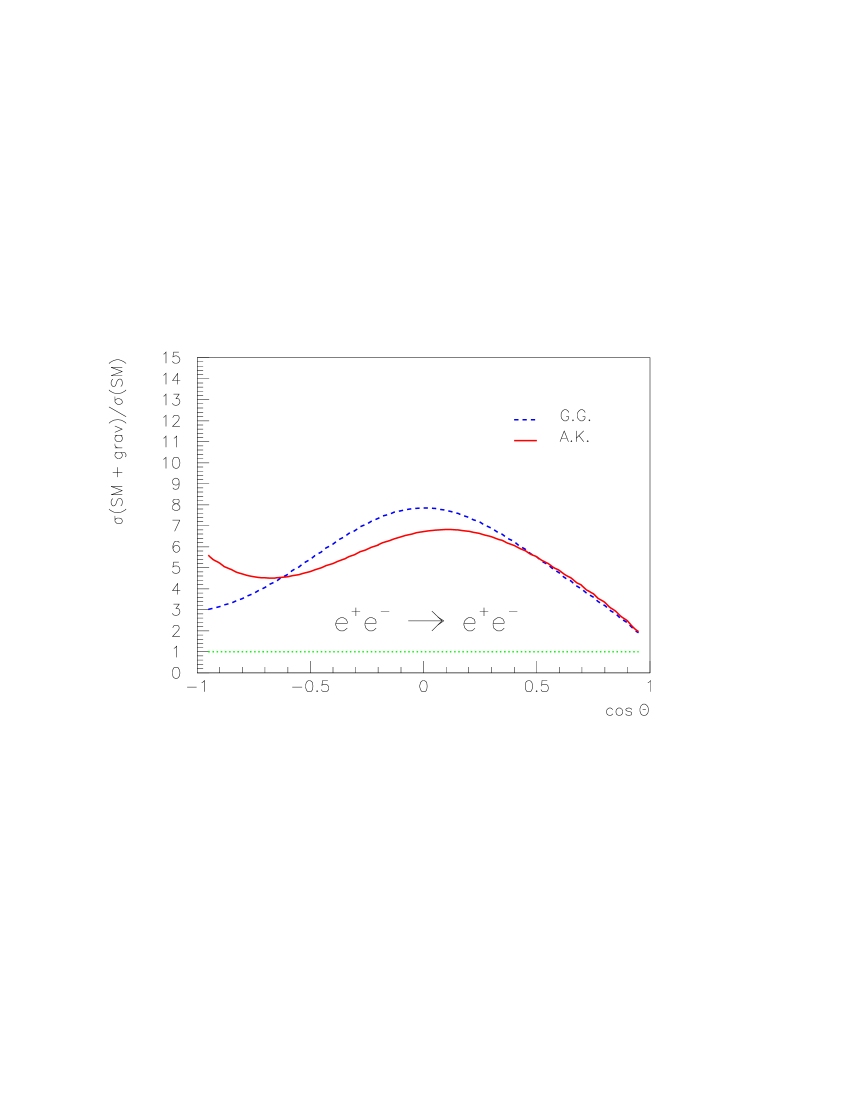
Figure 2: The same as in Fig. 1, except for the collision energy is equal to $\sqrt{s}=1$ TeV.

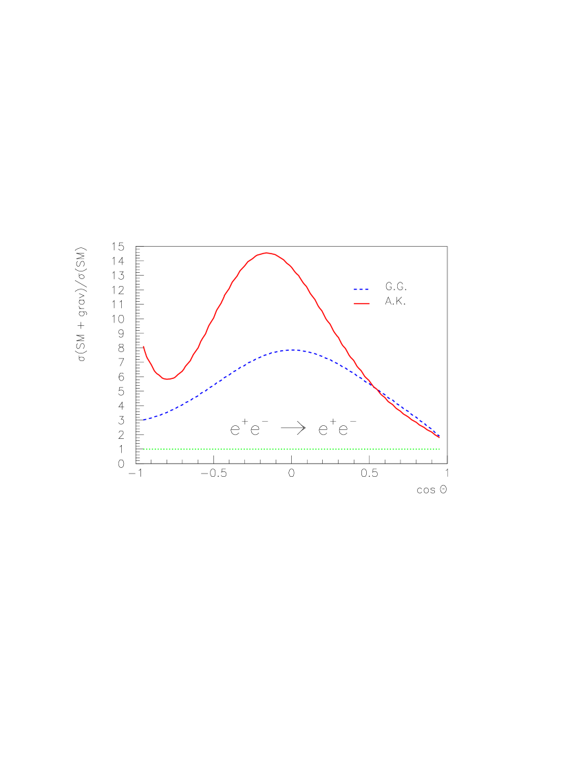
Figure 3: The same energy as in Fig. 2, with the parameters $M_{5}=1.8$ TeV, $\kappa=1$ GeV.

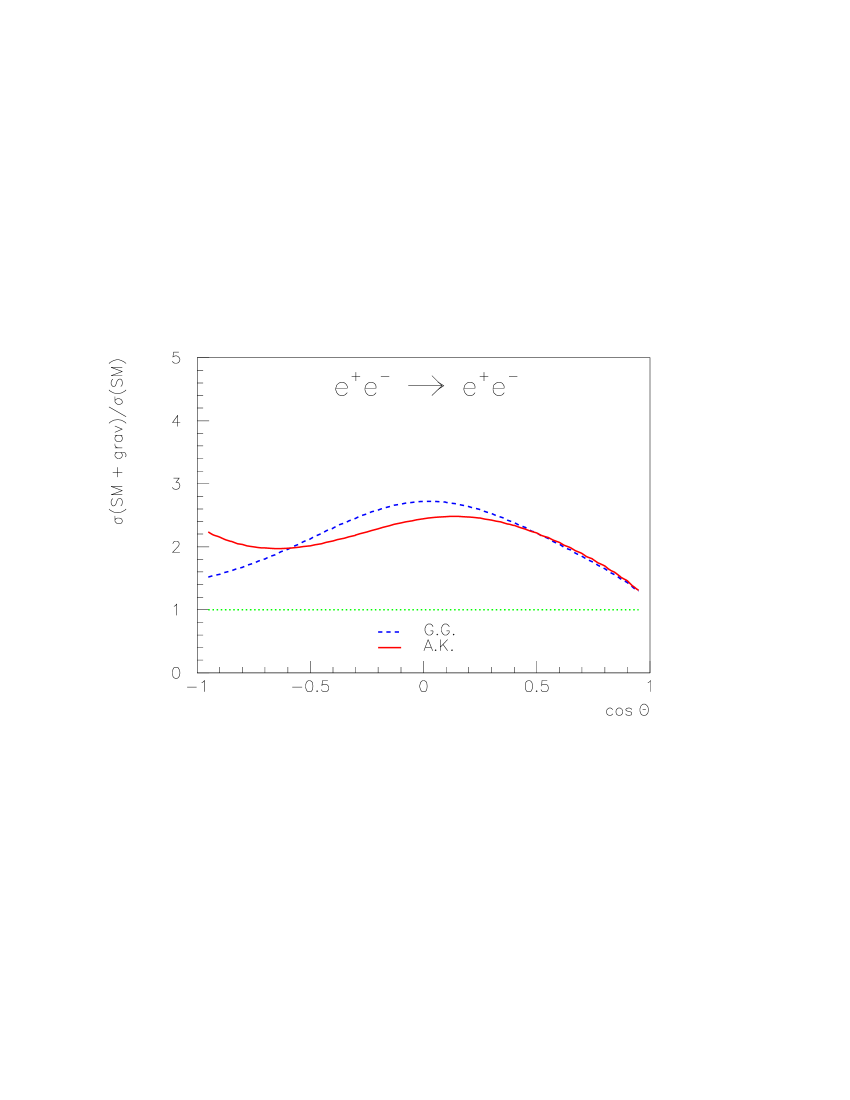
Figure 4: The same energy as in Fig. 2, with the parameters $M_{5}=2.5$ TeV, $\kappa=100$ MeV.

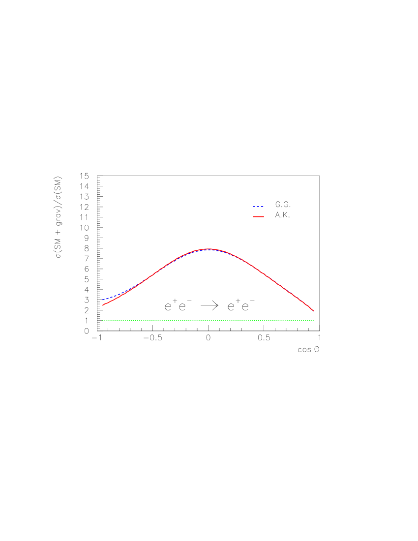
Figure 6: The same energy as in Fig. 2, with the parameters $M_{5}=1.8$ TeV, $\kappa=900$ MeV.

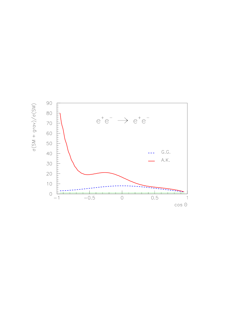
Figure 7: The same energy as in Fig. 2, with the parameters $M_{5}=1.8$ TeV, $\kappa=994$ MeV.

However, these two estimations (based on exact formula  (32) and approximate one (37), respectively) differ drastically when we consider a collision energy relevant for future linear colliders [16]. This is illustrated in Figs. 2–7. If we compare Figs. 6, 7 and 3, we conclude that at fixed value of $M_{5}$, the ratio of the total cross section to the SM cross section is very sensitive to variations of the curvature $\kappa$ within a narrow region (0.9 GeV – 1 GeV, in our case). The effect is less pronounced, but still significant, at larger $M_{5}$ (see Figs. 4, 5). Let us note that the interference of gravity with the SM forces is constructive in the Bhabha scattering, and the ratio $\sigma(\mathrm{SM+grav})/\sigma(\mathrm{SM})$ is lager than 1 for all cases.

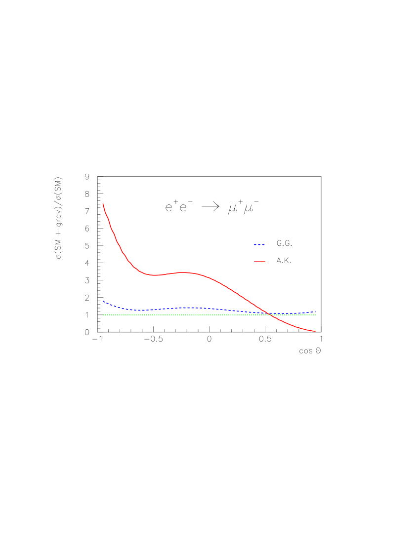
Figure 8: The virtual graviton contribution to the cross section of the process $e^{+}e^{-}\rightarrow\mu^{+}\mu^{-}$ as a function of the scattering angle. The collision energy $\sqrt{s}=1$ TeV. Both curves correspond to $M_{5}=1.8$ TeV, $\kappa=100$ MeV.

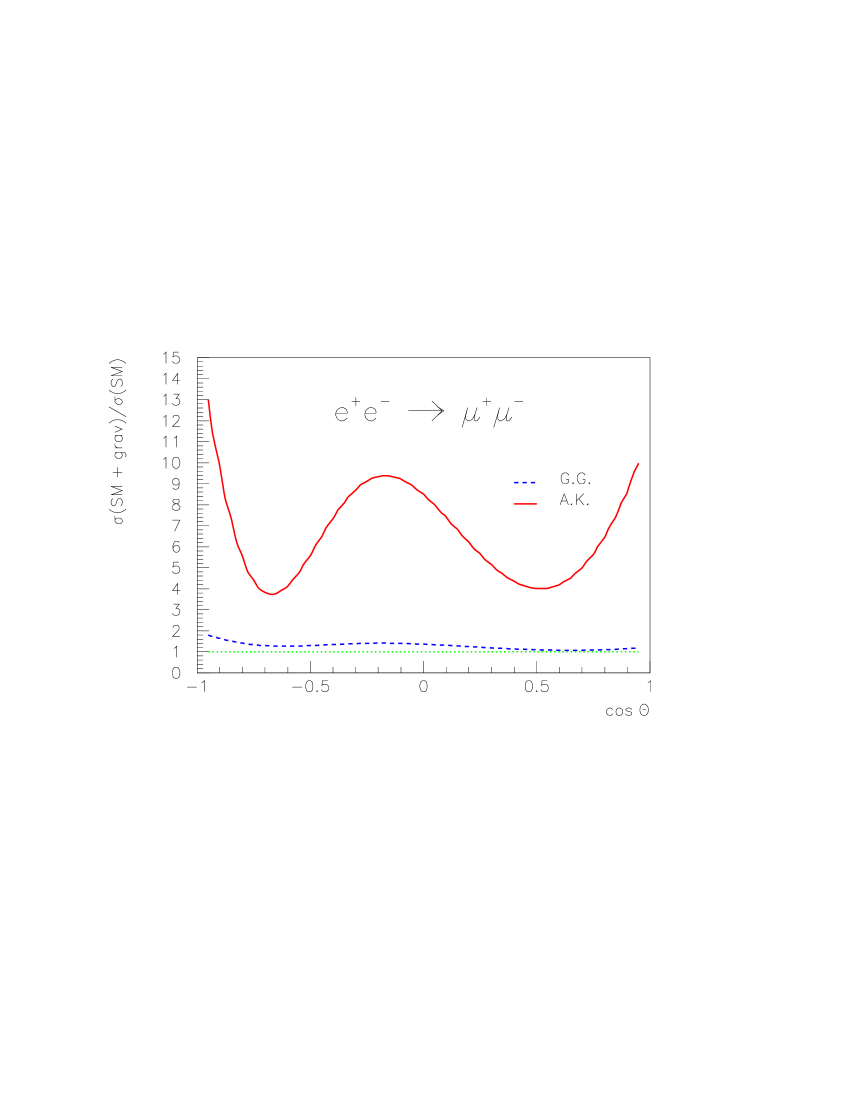
Figure 9: The same as in Fig. 8, with the parameters $M_{5}=1.8$ TeV, $\kappa=1$ GeV.

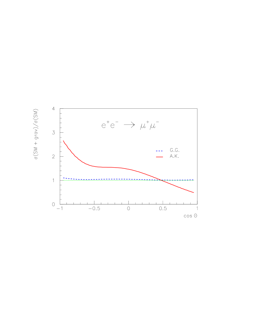
Figure 10: The same as in Fig. 8, with the parameters $M_{5}=2.5$ TeV, $\kappa=100$ GeV.

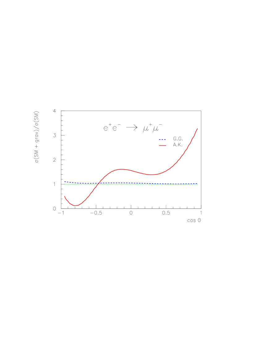
Figure 11: The same as in Fig. 8, with the parameters $M_{5}=2.5$ TeV, $\kappa=1$ GeV.

Now let us consider the process $e^{+}e^{-}\rightarrow\mu^{+}\mu^{-}$. The estimates show that the gravity effects are negligible at $\sqrt{s}=200$ GeV. Contrary to the Bhabha process, the gravity effects calculated with the use of approximate formulas (37) become very small at $M_{5}=2.5$ TeV (see Figs. 8–11). As for predictions based on the exact formula (32), they change both qualitatively and quantitatively with variations of the parameters of the RS model. To see this, it is enough to compare Figs. 8 and 9 ($\kappa$ changes from 100 MeV to 1 GeV, with $M_{5}$ being fixed), as well as Figs. 9 and 11 ($\kappa$ is fixed, while $M_{5}$ changes from 1.8 TeV to 2.5 TeV). The interference can be destructive or constructive, depending on $\cos\theta$ and values of the parameters.

3 Conclusions and discussions

In the present paper the contributions of the virtual $s$ and $t$-channel KK gravitons to the Bhabha scattering and to the process $e^{+}e^{-}\rightarrow\mu^{+}\mu^{-}$ at the LC energy $\sqrt{s}=1$ TeV were numerically estimated. We have considered the small curvature option of the RS model with two branes ($\kappa\ll\bar{M}_{5}$). In such a scheme, the KK graviton spectrum is the series of the narrow low-mass resonances. The SM fields live on the TeV brane, while the gravity propagates in the bulk.

The 5-dimensional Planck scale $M_{5}$ is taken to be 1.8 TeV and 2.5 TeV, with the curvature parameter being restricted to the region $\kappa=100\mathrm{\ MeV}\div 1\mathrm{\ GeV}$, that means $\sqrt{s}\sim M_{5}\gg\kappa$. For the numerical estimates, we used the formula for the process-independent gravity part of the scattering amplitude, $\mathcal{S}(s)$, from Ref. [9] (see Eq. (32)).

For comparison, we have made calculations by using Eqs. (37) which treat the spectrum of the KK graviton as the continuum. We have found that both expressions coincide only at the LEP2 energy, when the gravity effects appeared to be small. At the LC energy their predictions differ both qualitatively and quantitatively. It means that the sum in the KK number can not be approximated by integration over graviton mass. Moreover, the graviton widths should be properly taken into account, as formula (32) does.

In Figs. 2–7 the ratio $\sigma(\mathrm{SM+grav})/\sigma(\mathrm{SM})$ for the Bhabha process at collision energy $\sqrt{s}=1$ TeV is presented. Everywhere $\sigma(\mathrm{SM})$ means the SM differential cross section with respect to $\cos\theta$, while $\sigma(\mathrm{SM+grav})$ means the differential cross section which takes into account both the SM and gravity interactions.

In Figs. 8–11 our predictions for the process $e^{+}e^{-}\rightarrow\mu^{+}\mu^{-}$ are shown.

One should conclude that at fixed value of the gravity scale $M_{5}$, the cross section ratio is very sensitive even to the slight variations of the curvature $\kappa$ (compare, for instance, Figs. 6, 7 and 3, as well as Figs 8 and 9). The ratio $\sigma(\mathrm{SM+grav})/\sigma(\mathrm{SM})$ can reach tens at some values of the parameters (see Figs. 7, 9).

Such a behavior of the cross section ratios comes from the explicit form of the function $\mathcal{S}(s)$ (32). Indeed, at $\eta\,(\sqrt{s}/\bar{M}_{5})^{3}\ll 1$ the parameter $\varepsilon$ in Eq. (32) is much less than 1, and the function $\mathcal{S}(s)$ has a significant real part. There is an interference with the SM contributions, that results in a nontrivial dependence of $\sigma(\mathrm{SM+grav})/\sigma(\mathrm{SM})$ on $\cos\theta$. Given the approximation with zero real part is used (37), no interference terms exist, and $\cos\theta$-dependence of the cross section ratio becomes similar for all sets of the parameters (dashed curves in Figs. 2–11).

If the parameter $A=\sqrt{s}/\kappa+\pi/4$ in formula (32) obeys the equation $\cos A=0$, the denominator in (32) becomes small, and, correspondingly, the function $\mathcal{S}(s)$ becomes large. It results in the rapid variation of the gravity contribution near corresponding values of $\kappa$.

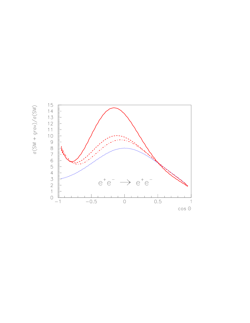
Figure 12: The dashed and dash-dotted lines correspond to smearing of gravity cross section in the interval $(\sqrt{s}-\Delta\sqrt{s},\sqrt{s}+\Delta\sqrt{s})$, with $\Delta\sqrt{s}=10$ GeV and $\Delta\sqrt{s}=50$ GeV, respectively, while the solid line corresponds to a case without energy smearing. The average energy $\sqrt{s}=1$ TeV, the parameters are the same as in Fig. 3. The dotted line is obtained in zero width approximation The number of resonances which lie within the energy resolution is equal to 6 (31) for $\Delta\sqrt{s}=10$ GeV ($50$ GeV).

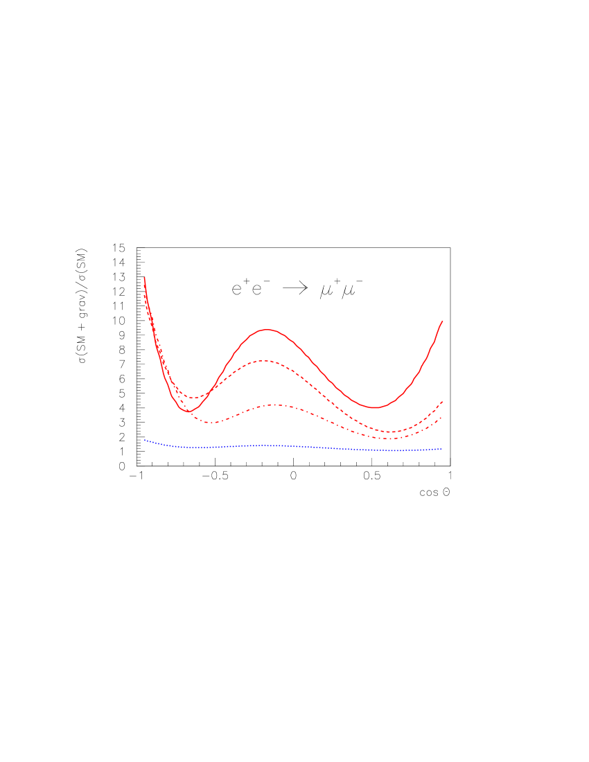
Figure 13: The same as in Fig. 12, but for the dimuon production with the parameters taken from Fig. 9. The number of resonances which lie within the energy resolution coincides with that in the previous figure.

All calculations (except for Fig. 1) were done for the fixed energy $\sqrt{s}=1$ TeV. However, the effects related with non-zero graviton widths remain significant after energy smearing within some interval around this value of $\sqrt{s}$, as one can see in Figs. 12, 13. Note that the energy smearing has a small influence on the cross section ratios for both processes in the region $\cos\theta<-0.8$.

It is worth to note that both a discrete character of the mass spectrum and nonzero widths of the KK gravitons are also important in a case of flat compact extra dimension, as it is shown in Appendix.

Appendix A

Let us demonstrate that the account of the graviton widths changes zero width result by considering a simpler case of one extra flat dimension [11]. The contribution of virtual $s$-channel KK gravitons is then defined by the quantity

$$\tilde{\mathcal{S}}(s)=\frac{1}{\bar{M}_{\mathrm{Pl}}^{2}}\sum_{n=1}^{\infty}\frac{1}{s-m_{n}^{2}+i\,m_{n}\Gamma_{n}}\;.$$ (A.1)

The reduced Planck mass is related with a 5-dimensional reduced gravity scale, $\bar{M}_{4+1}$, by the relation:

$$\bar{M}_{\mathrm{Pl}}^{2}=2\pi\bar{M}_{4+1}^{3}R_{c}\;,$$ (A.2)

with $R_{c}$ being the radius of the extra dimension. Remember that $\bar{M}_{4+1}=(2\pi)^{-1/3}M_{4+1}$ [4].

The masses of the KK gravitons are

$$m_{n}=\frac{n}{R_{c}},\qquad n=1,2\ldots\;,$$ (A.3)

while the graviton widths are given by [17]

$$\Gamma_{n}=\eta\,\frac{m_{n}^{3}}{\bar{M}_{\mathrm{Pl}}^{2}}\;.$$ (A.4)

The function $\tilde{\mathcal{S}}(s)$ (A.1) can be rewritten as

$$\tilde{\mathcal{S}}(s)=\frac{R_{c}^{4}}{i\eta}\,\frac{1}{b^{2}-a^{2}}\sum_{n=1}^{\infty}\left(\frac{1}{a^{2}-n^{2}}-\frac{1}{b^{2}-n^{2}}\right)\;,$$ (A.5)

where

$$a =\sqrt{s}R_{c}+\frac{i\eta}{2}\,\frac{s^{3/2}R_{c}}{\bar{M}_{\mathrm{Pl}}^{2}}\;,$$ (A.6)

$$b^{2} =-i\,\frac{\bar{M}_{\mathrm{Pl}}^{2}R_{c}^{2}}{\eta}\;.$$ (A.7)

Note that $|a|\simeq\sqrt{s}\,R_{c}\gg 1$, and $|b|\gg|a|$. In the region $\sqrt{s}\sim\bar{M}_{4+1}\ll\bar{M}_{\mathrm{Pl}}$, the second term in the sum (A.5) is non-leading, and we get (with negligible corrections of the type $\mathrm{O}(\sqrt{s}/\bar{M}_{\mathrm{Pl}})$ omitted):

$$\tilde{\mathcal{S}}(s)\simeq\frac{R_{c}^{2}}{\bar{M}_{\mathrm{Pl}}^{2}}\,\sum_{n=1}^{\infty}\frac{1}{a^{2}-n^{2}}\;.$$ (A.8)

The sum in Eq. (A.8) is known to be

$$\sum_{n=1}^{\infty}\frac{1}{a^{2}-n^{2}}=\frac{\pi}{2a}\,\cot(\pi a)-\frac{1}{2a^{2}}\;.$$ (A.9)

By using formulae

$$\cos(x+iy) =\cos x\cosh y-i\sin x\sinh y\;,$$

$$\sin(x+iy) =\sin x\cosh y+i\cos x\sinh y\;,$$ (A.10)

we get from Eqs. (A.8)-(Appendix A) and hierarchy relation (A.2):

$$\tilde{\mathcal{S}}(s)=\frac{1}{8\bar{M}_{4+1}^{3}\sqrt{s}}\;\frac{\sin 2B-i\sinh 2\delta}{\sin^{2}\!B+\sinh^{2}\!\delta}\;,$$ (A.11)

where

$$B=\pi R_{c}\sqrt{s}\;,\qquad\delta=\frac{\eta}{4}\Big{(}\frac{\sqrt{s}}{\bar{M}_{4+1}}\Big{)}^{3}\;.$$ (A.12)

As one can see from (A.11), a magnitude of the virtual graviton contribution is defined by the TeV scale $\bar{M}_{4+1}$, not by the Planck mass $\bar{M}_{\mathrm{Pl}}$. Moreover, the formula (A.11) is similar to formula (32) up to replacements $\bar{M}_{5}\rightarrow 2^{1/3}\bar{M}_{4+1}$, $\kappa\rightarrow 1/(\pi R_{c})$.

The real part of $\tilde{\mathcal{S}}(s)$ in Eq. (A.11) gives a small contribution after energy smearing due to its rapid oscillations in $\sqrt{s}$. The imaginary part of $\tilde{\mathcal{S}}(s)$ in Eq. (A.11) has a correct zero width limit ($\eta\rightarrow 0$), as one can easily check with the use of well-known formula

$$\frac{1}{\pi}\,\lim_{\epsilon\rightarrow 0}\frac{\epsilon}{x^{2}+\epsilon^{2}}=\delta(x)\;.$$ (A.13)

It also coincides with zero width expression in the trans-Planckian energy region, namely, at $\sqrt{s}>\bar{M}_{4+1}(4/\eta)^{1/3}\simeq 3.5\bar{M}_{4+1}$.

However, at $\sqrt{s}\lesssim 3.5\bar{M}_{4+1}$ the exact formula (A.11) and zero width formula result in different predictions by analogy with the RS scenario which has been considered in the present paper.

Let us underline that the so-called zero width formula is obtained under assumption that a set of the graviton resonances can be replaced by a continuous mass spectrum:

$$\tilde{\mathcal{S}}(s) =\frac{1}{\bar{M}_{\mathrm{Pl}}^{2}}\sum_{n=1}^{\infty}\frac{1}{s-m_{n}^{2}+i\,m_{n}\Gamma_{n}}$$

$$\rightarrow\frac{1}{\bar{M}_{\mathrm{Pl}}^{2}}\sum_{n=1}^{\infty}\frac{1}{s-m_{n}^{2}+i0}$$

$$\rightarrow-\frac{i\pi R_{c}}{\bar{M}_{\mathrm{Pl}}^{2}}\int\limits_{0}^{\infty}\!dm\,\delta(s-m^{2})=-\frac{i}{4\bar{M}_{4+1}^{3}\sqrt{s}}\;.$$ (A.14)

The last step in (Appendix A) is justified if only

$$\frac{1}{R_{c}}<\Gamma_{n}$$ (A.15)

is satisfied for relevant KK modes ($n\sim\sqrt{s}\,R_{c}$, in our case). This inequality is equivalent to the inequality $\sqrt{s}>\bar{M}_{4+1}(2\pi/\eta)^{1/3}\simeq 4\bar{M}_{4+1}$ already derived above.

Thus, one has to conclude that the approximate expression for $\tilde{\mathcal{S}}(s)$ (Appendix A) can be used only at $\sqrt{s}>4\bar{M}_{4+1}$. In the kinematical region $\sqrt{s}\lesssim 4\bar{M}_{4+1}$, the gravitons widths should be taken into account, and the KK sum (A.1) cannot be replaced by integration in graviton masses.

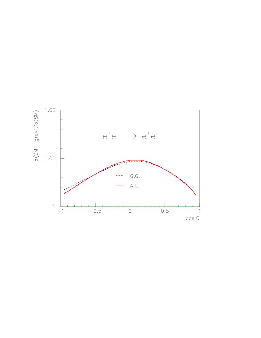
Figure 1: The correction to the Bhabha cross section resulting from virtual graviton exchanges as a function of the scattering angle at the LEP2 energy $\sqrt{s}=200$ GeV. The solid line is our prediction which takes into account both a discrete character of the spectrum and widths of the KK gravitons. The dashed line corresponds to the continuous mass approximation for the graviton spectrum [10]. The curves correspond to $M_{5}=1.8$ TeV and $\kappa=100$ MeV.

Figure 5: The same energy as in Fig. 2, with the parameters $M_{5}=2.5$ TeV, $\kappa=1$ GeV.

References

- [1] L. Randall and R. Sundrum, Phys. Rev. Lett. 83, 3370 (1999)
- [2] V.A. Rubakov, Phys. Usp. 44, 871 (2001)
- [3] E.E. Boos, Yu.A. Kubyshin,, M.N. Smolyakov and I.P. Volobuev, Class. Quan. Grav. 19, 4591 (2002); E.E. Boos, Yu.S. Mikhailov, M.N. Smolyakov and I.P. Volobuev, Nucl. Phys. B 717, 19 (2005)
- [4] G.F. Giudice, R. Rattazzi and J.D. Wells, Nucl. Phys. B 544, 3 (1999)
- [5] H. Davoudiasl, J.L. Hewett and T.G. Rizzo, Phys. Rev. D 63, 075004 (2001)
- [6] E. Gallo, Plenary talk at the ICHEP 2006, Moscow, July 26 - August 2, 2006
- [7] S. Shmatov, Talk at the ICHEP 2006, Moscow, July 26 - August 2, 2006
- [8] A.V. Kisselev and V.A. Petrov, Phys. Rev. D 71, 124032 (2005)
- [9] A.V. Kisselev, Phys. Rev. D 73, 024007 (2006)
- [10] G.F. Giudice, T. Plehn and A. Strumia, Nucl. Phys. B 706, 455 (2005)
- [11] N. Arkani-Hamed, S. Dimopoulos and G. Dvali, Phys. Lett. B 429 (1998) 263; I. Antoniadis, N. Arkani-Hamed, S. Dimopoulos and G. Dvali, Phys. Lett. B 436 (1998) 257 ; N. Arkani-Hamed, S. Dimopoulos and G. Dvali, Phys. Rev. D 59 (1999) 086004
- [12] A.V. Kisselev and V.A. Petrov, Eur. Phys. J. C 36 (2004) 103.
- [13] K. Klein, Talk at the ICHEP 2006, Moscow, July 26 - August 2, 2006
- [14] G.N. Watrson, Treatise on the theory of Bessel functions (McMillan, New York, 1922)
- [15] A.V. Kisselev, Eur. Phys. J. C 42, 217 (2005)
- [16] T. Abe et al., American Linear Collider Group, hep-ex/0106057; J.A. Aguliar-Saavedra et al., ECFA/DESY LC Physics Working Group, hep-ph/0106315; T. Abe et al., ACFA Linear Collider Working Group, hep-ph/0109166; G. Laow et al., ILC Technical Review Committee, second report, 2003, SLAC-R-606
- [17] T. Han, J.D. Lykken and R.-J. Zhang, Phys. Rev. D 59, 105006 (1999)