KK Gravitons and Unitarity Violation in the Randall-Sundrum Model

Abstract

We show that perturbative unitarity for $W_{L}^{+}W_{L}^{-}\to W_{L}^{+}W_{L}^{-}$ scattering places significant constraints on the Randall-Sundrum theory with two 3-branes, with matter confined to the TeV brane. The exchange of massive 4D Kaluza-Klein gravitons leads to amplitudes growing linearly with the CM energy squared. Summing over KK gravitons up to a scale $\overline{\Lambda}$ and testing unitarity at $\sqrt{s}=\overline{\Lambda}$, one finds that unitarity is violated for $\overline{\Lambda}$ below the ’naive dimensional analysis’ scale, $\Lambda_{\rm NDA}$. We evaluate $\overline{\Lambda}$ as a function of the curvature ratio $m_{0}/m_{Pl}$ for the pure gravity theory. We then demonstrate that unitarity need not be violated at $\overline{\Lambda}$ in the presence of a heavy Higgs boson. In fact, much larger Higgs masses are consistent with unitarity than if no KK gravitons are present. Observation of the mass and width (or cross section) of one or more KK gravitons at the LHC will directly determine $m_{0}/m_{Pl}$ and the scale $\widehat{\Lambda}_{W}$ specifying the couplings of matter to the KK gravitons. With this information in hand and a measurement of the Higgs boson mass, one can determine the precise scale $\overline{\Lambda}$ below which unitarity will remain valid.

I Introduction

The Standard Model (SM) of electroweak interactions is confirmed by all existing experimental data. However the model suffers from certain theoretical drawbacks. One of these is the hierarchy problem: namely, the SM can not consistently accommodate the weak energy scale ${\cal O}(1~{}{\rm TeV})$ and a much higher scale such as the Planck mass scale ${\cal O}(10^{19}~{}{\rm GeV})$. Therefore, it is commonly believed that the SM is only an effective theory emerging as the low-energy limit of some more fundamental high-scale theory that presumably could contain gravitational interactions.

Models that involve extra spatial dimensions could provide a solution to the hierarchy problem. One attractive proposal was formulated by Randall and Sundrum (RS)  Randall:1999ee . They postulate a 5D universe with two 4D surfaces (“3-branes”). All the SM particles and forces with the exception of gravity are assumed to be confined to one of those 3-branes called the visible or TeV brane. Gravity lives on the visible brane, on the second brane (the “hidden brane”) and in the bulk. All mass scales in the 5D theory are of order of the Planck mass. By placing the SM fields on the visible brane, all the order Planck mass terms are rescaled by an exponential suppression factor (the “warp factor”) $\Omega_{0}\equiv e^{-m_{0}b_{0}/2}$, which reduces them down to the weak scale ${\cal O}(1~{}{\rm TeV})$ on the visible brane without any severe fine tuning. To achieve the necessary suppression, one needs $m_{0}b_{0}/2\sim 35$. This is a great improvement compared to the original problem of accommodating both the weak and the Planck scale within a single theory. The RS model is defined by the 5-D action:

$$S = -\int d^{4}x\,dy\sqrt{-\widehat{g}}\left({2M_{Pl\,5}^{3}\widehat{R}}+\Lambda\right)$$ (1)

$$+\int d^{4}x\,\sqrt{-g_{\rm hid}}({\cal L}_{\rm hid}-V_{\rm hid})+\int d^{4}x\,\sqrt{-g_{\rm vis}}({\cal L}_{\rm vis}-V_{\rm vis})\,,$$

where the notation is self-explanatory, see also Dominici:2002jv for details. In order to obtain a consistent solution to Einstein’s equations corresponding to a low-energy effective theory that is flat, the branes must have equal but opposite cosmological constants and these must be precisely related to the bulk cosmological constant; $V_{\rm hid}=-V_{\rm vis}={24M_{Pl\,5}^{3}m_{0}}\;\;\;\;\;$ and $\;\;\;\;\;\Lambda=-{24M_{Pl\,5}^{3}m_{0}^{2}}$. With these choices, the following metric is a solution of Einstein’s equations:

$$\widehat{g}_{\widehat{\mu}\widehat{\nu}}(x,y)=\left(\begin{array}[]{ccc}e^{-2m_{0}b_{0}|y|}\eta_{\mu\nu}&|&0\\ \hline\cr 0&|&-b_{0}^{2}\end{array}\right)\,.$$ (2)

After an expansion around the background metric we obtain the gravity-matter interactions

$${\cal L}_{\rm int}=-{1\over\widehat{\Lambda}_{W}}\sum_{n\neq 0}h_{\mu\nu}^{n}T^{\mu\nu}-{\phi_{0}\over\Lambda_{\phi}}T_{\mu}^{\mu}$$ (3)

where $h_{\mu\nu}^{n}(x)$ are the Kaluza-Klein (KK) modes (with mass $m_{n}$) of the graviton field $h_{\mu\nu}(x,y)$, $\phi_{0}(x)$ is the radion field (the quantum degree of freedom associated with fluctuations of the distance between the branes), $\widehat{\Lambda}_{W}\simeq\sqrt{2}m_{Pl}\Omega_{0}$, where $\Omega_{0}=e^{-m_{0}b_{0}/2}$, and $\Lambda_{\phi}=\sqrt{3}\,\widehat{\Lambda}_{W}$. To solve the hierarchy problem, $\widehat{\Lambda}_{W}$ should be of order $1-10~{}{\rm TeV}$, or perhaps higher Randall:1999ee . Note from Eq. (3) that the radion couples to matter with coupling strength $1/\Lambda_{\phi}$. In addition to the radion, the model contains a conventional Higgs boson, $h_{0}$. The RS model solves the hierarchy problem by virtue of the fact that the 4D electro-weak scale is given in terms of the ${\cal O}(m_{Pl})$ 5D Higgs vev, $\widehat{v}$, by:

$$v_{0}=\Omega_{0}\widehat{v}=e^{-m_{0}b_{0}/2}\widehat{v}\sim 1~{}{\rm TeV}\;\;\;\;\;{\rm for}\;\;\;\;\;m_{0}b_{0}/2\sim 35\,.$$ (4)

However, the RS model is trustworthy in its own right only if the 5D curvature $m_{0}$ is small compared to the 5D Planck mass, $M_{Pl\,5}$ Randall:1999ee . The reason is that for higher $m_{0}$ one can’t trust the RS solution of Einstein’s equations since then $m_{0}$, a parameter of the solution, is greater than the scale up to which classical gravity can be trusted. The $m_{0}<M_{Pl\,5}$ requirement and the fundamental RS relation $m_{Pl}^{2}=2M_{Pl\,5}^{3}/m_{0}$ imply that $m_{0}/m_{Pl}=2^{-1/2}(m_{0}/M_{Pl\,5})^{3/2}$ should be significantly smaller than 1. Roughly, it is believed that $m_{0}/m_{Pl}\mathrel{\raise 1.29167pt\hbox{$<$\kern-7.5pt\lower 4.30554pt\hbox{$\sim$}}}0.1$ is required for internal consistency of the RS 5D model. String theory estimates are usually smaller, typically of order $m_{0}/m_{Pl}\sim 0.01$ Davoudiasl:1999jd . At the same time, the effective 4D RS theory should be well behaved up to some maximum energy that can be estimated in a number of ways. One estimate of the maximum energy scale is that obtained using the ’naive dimensional analysis’ (NDA) approach Manohar:1983md , and the associated scale is denoted $\Lambda_{\rm NDA}$.  One finds

$$\Lambda_{\rm NDA}=2^{7/6}\pi(m_{0}/m_{Pl})^{1/3}\widehat{\Lambda}_{W}\,,$$ (5)

where $\widehat{\Lambda}_{W}$ was defined in Eq. (3); its inverse sets the strength of the coupling between matter and gravitons. We emphasize that $\Lambda_{\rm NDA}$ is obtained when the exchange of the whole tower of KK modes up to $\Lambda_{\rm NDA}$ is taken into account.  Physically, $\Lambda_{\rm NDA}$ is the energy scale at which the theory starts to become strongly coupled and string/$M$-theoretic excitations appear from a 4D observer’s point of view  Randall:1999ee . Above $\Lambda_{\rm NDA}$, the RS effective theory is expected to start to break down and additional new physics must emerge. An interesting question is whether the model violates other theoretical constraints at this same scale, a lower scale, or if everything is completely consistent for energy scales below $\Lambda_{\rm NDA}$. In this paper, we show that unitarity in the $J=0$ partial wave of $W_{L}^{+}W_{L}^{-}\to W_{L}^{+}W_{L}^{-}$ scattering is always violated in the RS model for energies below the $\Lambda_{\rm NDA}$ scale. We will define $\overline{\Lambda}$ as the largest $\sqrt{s}$ value such that if we sum over graviton resonances with mass below $\overline{\Lambda}$ (but do not include diagrams containing the Higgs boson or radion of the model) then $W_{L}^{+}W_{L}^{-}\to W_{L}^{+}W_{L}^{-}$ scattering remains unitary in the $J=0,1,2$ partial waves. We find that $\overline{\Lambda}$ depends upon the curvature ratio, $m_{0}/m_{Pl}$, in much the same manner as $\Lambda_{\rm NDA}$, but is always $<\Lambda_{\rm NDA}$. The latter implies that $\overline{\Lambda}$ is a more precise estimate of the energy scale at which the theory becomes strongly interacting.

The maximum energy scale determined from $W_{L}^{+}W_{L}^{-}\to W_{L}^{+}W_{L}^{-}$ scattering unitarity if a light Higgs boson is included is essentially the same as $\overline{\Lambda}$ (and is essentially independent of the radion mass assuming no Higgs radion mixing). However, the presence of a heavy Higgs boson can delay the onset of unitarity violation in $W_{L}^{+}W_{L}^{-}\to W_{L}^{+}W_{L}^{-}$ to energies above $\overline{\Lambda}$. As a result, the question arises as to whether we should continue to cutoff our KK sums at a maximum mass equal to the $\overline{\Lambda}$ obtained for the $J=0$ partial wave before inclusion of Higgs and radion contributions. Alternative choices include using the $\overline{\Lambda}$ obtained using the $J=1$ or $J=2$ partial waves, for which Higgs and radion exchanges are less important; see later plots in Fig. 3. One could also consider using the $\overline{\Lambda}$ determined by unitarity violation of the scattering amplitudes for transversely polarized vector bosons, where it is known Han:2004wt that the leading contribution ($\propto s$) originates purely from graviton exchange.  Each of these choices yields a somewhat different maximum $\sqrt{s}$ value (always modestly higher than the $\overline{\Lambda}$ obtained for $J=0$ and KK exchanges only). We have opted to always cut off our sums over KK resonances for masses above the $\overline{\Lambda}$ obtained for $J=0$ with KK exchanges only. This will provide a conservative estimate of the influence of KK resonance exchanges on unitarity limits.

As will be discussed later, observation of even one KK graviton and its width or hadron-collider cross section will determine both $\widehat{\Lambda}_{W}$ and $m_{0}/m_{Pl}$, from which $\overline{\Lambda}$ can be determined. If the Higgs boson mass is also known, one can then make a fairly precise determination of the $\sqrt{s}$ scale for which unitarity constraints are still obeyed for the given $\widehat{\Lambda}_{W}$, $m_{0}/m_{Pl}$ and Higgs mass and how this scale relates to $\overline{\Lambda}$.

In this paper, we will not consider the possible extension of the RS model obtained by including mixing between gravitational and electroweak degrees of freedom Giudice:2000av ; Dominici:2002jv . These can substantially amplify the radion contribution to $WW$ scattering (see Grzadkowski:2005tx ). However in the absence of such mixing, the $\phi_{0}$ and $h_{0}$ are mass eigenstates,  which we denote as $\phi$ and $h$. An important parameter is the quantity

$$R^{2}\equiv\widehat{g}_{VVh}^{2}+\widehat{g}_{VV\phi}^{2}=\widehat{g}_{ffh}^{2}+\widehat{g}_{ff\phi}^{2}=1+\gamma^{2}\,,$$ (6)

where the $\widehat{g}~{}$’s are defined Dominici:2002jv relative to SM Higgs coupling strength (e.g. $\widehat{g}_{WWh}=g_{WWh}/(gm_{W})$) and $\gamma\equiv v_{0}/\Lambda_{\phi}$ is $\ll 1$ for typical $\Lambda_{\phi}$ choices (with $v_{0}=246~{}{\rm GeV}$).

The $h$, the $\phi$ and the KK gravitons (generically denoted $G$) must all be considered in computing the high energy behavior of a process such as $W_{L}^{+}W_{L}^{-}\to W_{L}^{+}W_{L}^{-}$ scattering. As usual, there is a cancellation between scalar ($h$ and $\phi$) exchanges and gauge boson exchanges that leads to an amplitude ${\cal A}_{W_{L}^{+}W_{L}^{-}\to W_{L}^{+}W_{L}^{-}}$ that obeys  unitarity constraints (in particular, $|{\rm Re}a_{0}|\leq 1/2$ for the $J=0$ partial wave) so long as $m_{h}\mathrel{\raise 1.29167pt\hbox{$<$\kern-7.5pt\lower 4.30554pt\hbox{$\sim$}}}870~{}{\rm GeV}$. However, each KK resonance with mass below $\sqrt{s}$ will give a contribution to ${\cal A}_{W_{L}^{+}W_{L}^{-}\to W_{L}^{+}W_{L}^{-}}$ that grows with $s$, and, since the number of such KK resonances increases as the energy increases, their net effect does not decouple, and, in fact, becomes increasingly important as $\sqrt{s}$ increases. Thus, unitarity can easily be violated for rather modest energies. Unitarity in the context of the RS model has also been discussed in Han:2001xs and Choudhury:2001ke .

The paper is organized as follows. Sec. II presents leading analytical results for the partial wave amplitudes in the context of the RS model. Sec. III discusses the parameters of the model, including graviton widths, and experimental limits on these parameters. Sec. IV is devoted to detailed numerical analysis. Sec. V discusses the means for using future experiments to determine the model parameters. A summary and some concluding remarks are given in Sec. VI.

II Vector boson scattering and KK exchanges

Let us begin by reviewing the limit on the Higgs-boson mass in the SM obtained by requiring that $W_{L}^{+}W_{L}^{-}\to W_{L}^{+}W_{L}^{-}$ scattering be unitary at high energy. The constraint arises when we consider the elastic scattering of longitudinally polarized $W$ bosons. The amplitude can be decomposed into partial wave contributions: $T(s,\cos\theta)=16\pi\sum_{J}(2J+1)a_{J}(s)P_{J}(\cos\theta)$, where $a_{J}(s)=\frac{1}{32\pi(2J+1)}\int_{-1}^{1}T(s,\cos\theta)P_{J}(\cos\theta)d\cos\theta\,.$ In the SM, the partial wave amplitudes take the asymptotic form $a_{J}=A_{J}\left(\frac{s}{m_{W}^{2}}\right)^{2}+B_{J}\left(\frac{s}{m_{W}^{2}}\right)+C_{J}\,,$ where $s$ is the center-of-mass energy squared. Contributions that are divergent in the limit $s\to\infty$ appear only for $J=0$, 1 and 2. The $A$-terms vanish by virtue of gauge invariance, while, as is very well known, the $B$-term for $J=1$ and $0$ ($B_{2}=0$) arising from gauge interaction diagrams is canceled by Higgs-boson exchange diagrams. In the high-energy limit, the result is that $a_{J}$ asymptotes to an $m_{h}$-dependent constant. Imposing the unitarity limit of $|{\rm Re}~{}a_{J}|<1/2$ implies the Lee-Quigg-Thacker bound Lee:1977eg for the Higgs boson mass: $m_{h}\mathrel{\raise 1.29167pt\hbox{$<$\kern-7.5pt\lower 4.30554pt\hbox{$\sim$}}}870~{}{\rm GeV}$.

We will show that within the RS model $W_{L}^{+}W_{L}^{-}\to W_{L}^{+}W_{L}^{-}$ scattering violates unitarity in the $J=0$ partial wave at an energy scale below $\Lambda_{\rm NDA}$ when KK graviton exchanges are included. The various contributions to the amplitude are given in Table 1. From the table, we see that in the SM, obtained by setting $R^{2}=1$, the gauge boson contributions and Higgs exchange contributions cancel at ${\cal O}(s^{2})$ and ${\cal O}(s^{1})$. Regarding $G$ exchange contributions, we note that the apparent singularity in the $\cos\theta$ integral of the leading ${\cal O}(s)$ t-channel $G$ exchange is regularized by the graviton mass and width (neglected in the table).

diagram	${\cal O}(\frac{s^{2}}{v^{4}})$	${\cal O}(\frac{s^{1}}{v^{2}})$
$\gamma,Z$ s-channel	$-\frac{s^{2}}{g^{2}v^{4}}4\cos\theta$	$-\frac{s}{v^{2}}\cos\theta$
$\gamma,Z$ t-channel	$-\frac{s^{2}}{g^{2}v^{4}}(-3+2\cos\theta+\cos^{2}\theta)$	$-\frac{s}{v^{2}}\frac{3}{2}(1-5\cos\theta)$
$WWWW$ contact	$-\frac{s^{2}}{g^{2}v^{4}}(3-6\cos\theta-\cos^{2}\theta)$	$-\frac{s}{v^{2}}2(-1+3\cos\theta)$
$G$ s-channel	$0$	$-\frac{s}{24\widehat{\Lambda}_{W}^{2}}(-1+3\cos^{2}\theta)$
$G$ t-channel	$0$	$-\frac{s}{24\widehat{\Lambda}_{W}^{2}}\frac{13+10\cos\theta+\cos^{2}\theta}{-1+\cos\theta}$
$(h-\phi)$ s-channel	$0$	$-\frac{s}{v^{2}}R^{2}$
$(h-\phi)$ t-channel	$0$	$-\frac{s}{v^{2}}\frac{-1+\cos\theta}{2}R^{2}$

Table 1: The leading contributions to the $W_{L}^{+}W_{L}^{-}\to W_{L}^{+}W_{L}^{-}$ amplitude, where $R^{2}$ is defined in the text. $G$ denotes a single KK graviton.

It is worth noting that even though the graviton exchange amplitude has the same amplitude growth $\propto s$ as the SM vector boson and contact interactions, its angular dependence is different ($J=2$ vs. $J=1$); therefore, the graviton cannot act in place of the Higgs boson to restore correct high-energy unitary behavior for $a_{0}$ and $a_{1}$. It is also noteworthy that the $t$-channel graviton contributions to the $a_{J}$ are quite substantial as a result of the $(1-\cos\theta)^{-1}$ structure that is regulated by the graviton mass and width.

As is well known, the cancellation of the ${\cal O}(s^{2})$ contributions in Table 1 between the contact term and $s$- and $t$-channel gauge-boson exchange diagrams is guaranteed by gauge invariance. Even more remarkable is the cancellation of the most divergent graviton exchange terms. Indeed, a naive power counting shows that the graviton exchange can yield terms at ${\cal O}(s^{5})$, while the actual calculation shows that only the linear term $\propto s$ survives; all the terms with faster growth of ${\cal O}(s^{5},s^{4},s^{3},s^{2})$ cancel. The mechanism behind the cancellation is as follows. In the high-energy region the massive graviton propagator grows with energy as $k_{\mu}k_{\nu}k_{\alpha}k_{\beta}k^{-2}$, where $k$ is the momentum carried by the graviton, which will be of order $\sqrt{s}$. The graviton couples to the energy-momentum tensor $T_{\mu\nu}$, so the amplitude for a single graviton exchange is of the form $T_{\mu\nu}D^{\mu\nu,\alpha\beta}T_{\alpha\beta}\,.$ Since the energy-momentum tensor is conserved, $k^{\mu}T_{\mu\nu}=0$, terms in the numerator of the graviton propagator proportional to the momentum don’t contribute. (Note that for this argument to apply, all the external particles must be on their mass shell.) This removes two potential powers of $s$ in the amplitude. In order to understand the disappearance of two additional powers of $s$, let us calculate the energy-momentum tensor for the final state consisting of a pair of longitudinal $W$ bosons. A direct calculation reveals the following form of the $4\times 4$ tensor:

$$\langle 0|T^{\mu\nu}|W_{L}^{+}W_{L}^{-}\rangle=\left(\begin{array}[]{cccc}0&0&0&0\\ 0&\frac{1}{6}[(1-2\beta_{W})d^{0}_{0,0}+2(\beta_{W}-2)d^{2}_{0,0}]s&0&-\frac{1}{\sqrt{6}}(s+4m_{W}^{2})d^{2}_{1,0}\\ 0&0&-\frac{1}{2}sd^{0}_{0,0}&0\\ 0&-\frac{1}{\sqrt{6}}(s+4m_{W}^{2})d^{2}_{1,0}&0&-\frac{1}{6}[(1+\beta_{W})d^{0}_{0,0}+2(\beta_{W}-2)d^{2}_{0,0}]s\,,\end{array}\right)$$ (7)

in the reference frame in which the off-shell graviton is at rest. The scattering angle is measured relative to the direction of motion of the $W^{-}$, $d^{J}_{\mu\mu^{\prime}}(\cos\theta)=d^{J}_{\mu\mu^{\prime}}$ stands for the Wigner $d$ function and $\beta_{W}\equiv 1-4m_{W}^{2}/s$. Note that the factor $1/m_{W}^{2}$, which comes from the vector boson polarization vectors, has been canceled by two powers of $m_{W}$ coming from on-shellness of the longitudinal vector bosons, i.e. $m_{W}^{2}$ replaces an $s$ that originates from $T^{\mu\nu}$. In short, when the two vertices are contracted with the propagator of the virtual graviton, four potential powers of $s$ disappear leading to a single power of $s$. These arguments apply equally to $s$- and $t$-channel diagrams.

From the terms $\propto s$ and $\propto constant$ in the amplitude, one obtains the leading terms in the partial wave amplitudes that are $\propto s$, $\propto\ln s$, and $\propto constant$. We give below the leading terms deriving from a single KK graviton, the SM vector bosons and the $\phi-h$ exchanges (for the $J=2$, $1$ and $0$ partial waves):

$$a_{2} = -\frac{1}{960\pi\widehat{\Lambda}_{W}^{2}}\Biggl{\{}\left[91+30\log\left(\frac{m_{G}^{2}}{s}\right)\right]s+\left[241+210\log\left(\frac{m_{G}^{2}}{s}\right)\right]m_{G}^{2}+32g^{2}v^{2}\Biggr{\}}+{\cal O}(s^{-1})$$ (8)

$$a_{1} = -\frac{1}{1152\pi\widehat{\Lambda}_{W}^{2}}\Biggl{\{}\left[73+36\log\left(\frac{m_{G}^{2}}{s}\right)\right]s+36\left[1+3\log\left(\frac{m_{G}^{2}}{s}\right)\right]m_{G}^{2}+37g^{2}v^{2}\Biggr{\}}$$

$$\quad\qquad+\frac{1}{96\pi}\left[\frac{s}{v^{2}}(1-R^{2})-R^{2}g^{2}+\frac{12\cos^{2}\theta_{W}-1}{2\cos^{2}\theta_{W}}g^{2}\right]+{\cal O}(s^{-1})$$

$$a_{0} = -\frac{1}{384\pi\widehat{\Lambda}_{W}^{2}}\Biggl{\{}\left[11+12\log\left(\frac{m_{G}^{2}}{s}\right)\right]s-\left[10-12\log\left(\frac{m_{G}^{2}}{s}\right)\right]m_{G}^{2}+19g^{2}v^{2}\Biggr{\}}$$ (10)

$$\qquad\quad+\frac{1}{32\pi}\left[\frac{s}{v^{2}}(1-R^{2})+R^{2}g^{2}-4\frac{\overline{m}_{\rm scal}^{2}}{v^{2}}\right]+{\cal O}(s^{-1})\,,$$

where $\overline{m}_{\rm scal}^{2}=\widehat{g}_{VVh}^{2}m_{h}^{2}+\widehat{g}_{VV\phi}^{2}m_{\phi}^{2}$ is equal to $m_{h}^{2}+\gamma^{2}m_{\phi}^{2}$ in the absence of Higgs-radion mixing. It is amusing to note that in the case of $a_{2}$, the $s$-channel contribution is quite minor, contributing just $a_{2}\ni-\frac{1}{960\pi\widehat{\Lambda}_{W}^{2}}$ to Eq. (8). Of course, one should sum over all relevant KK gravitons. We include all KK states with $m_{n}\leq\overline{\Lambda}$, where, as stated earlier, $\overline{\Lambda}$ will be taken to be the largest energy or mass scale for which $W_{L}^{+}W_{L}^{-}\to W_{L}^{+}W_{L}^{-}$ scattering remains unitarity in all partial waves before taking into account $h$ and $\phi$ exchanges. It is important to note that in our calculations the full sum over all modes with $m_{n}\leq\overline{\Lambda}$ will be included even when considering $\sqrt{s}$ values above or below $\overline{\Lambda}$ .

In our numerical results, we employ exact expressions for the $h$, $\phi$ and all KK contributions to $a_{0,1,2}$. Nonetheless, some analytic understanding is useful. We focus on $a_{0}$. Eq. (10) shows that the Higgs plus gauge boson contributions in the SM limit (obtained by taking $R^{2}=1$ and $\overline{m}_{\rm scal}^{2}=m_{h}^{2}$) combine to give a negative constant value at large $s$. If we add the radion, but neglect the KK graviton exchanges, then the leading terms for $a_{0}$ are:

$$a_{0}=\frac{1}{32\pi}\left[f(s)+g^{2}R^{2}-4\frac{\overline{m}_{\rm scal}^{2}}{v^{2}}\right],\,$$ (11)

where Dominici:2002jv ; Han:2001xs $f(s)=\frac{s}{v^{2}}(1-R^{2})=-\frac{s}{\Lambda_{\phi}^{2}}$ in the absence of Higgs-radion mixing. The negative signs for $f(s)$ and in front of $\overline{m}_{\rm scal}^{2}$ imply some amplification of unitarity-violation in the $\sim~{}{\rm TeV}$ energy range as compared to that which is present in the SM for large $m_{h}$ values. However, given the $1/(32\pi)$ factor and the fact that we typically consider $\sqrt{s}$ values of order $\Lambda_{\rm NDA},\widehat{\Lambda}_{W},\Lambda_{\phi}$ or below, this residual unitarity-violating behavior is never a dominant effect when the Higgs-radion mixing Grzadkowski:2005tx is neglected. Ultimately, at higher $\sqrt{s}$ values near $\overline{\Lambda}$ it is usually the purely KK graviton exchanges that dominate. From the asymptotic formula for $a_{0}$, a KK graviton with mass significantly below $\sqrt{s}$ enters ${\rm Re}~{}a_{0}$ with a positive sign. The sum of all these contributions is very substantial if $m_{0}/m_{Pl}$ is small.

III Parameters of the Model and Experimental Limits

At this point, it is useful to specify more fully the characteristics of the KK graviton excitations. We start with the parameters of the RS model: $\widehat{\Lambda}_{W}\simeq\sqrt{2}m_{Pl}\Omega_{0}$ (and $\Lambda_{\phi}=\sqrt{3}\widehat{\Lambda}_{W}$) and the curvature $m_{0}$. In terms of these, one finds $m_{n}=m_{0}x_{n}\Omega_{0}$, where $m_{n}$ is the mass of the $n$-th graviton KK mode and the $x_{n}$ are the zeroes of the Bessel function $J_{1}$ ($x_{1}\sim 3.8$, $x_{n}\sim x_{1}+\pi(n-1)$). A useful relation following from these equations is:

$$m_{n}=x_{n}{m_{0}\over m_{Pl}}{\Lambda_{\phi}\over\sqrt{6}}\,,\quad\mbox{implying}\quad m_{1}=15.5~{}{\rm GeV}\times\left({m_{0}/m_{Pl}\over 0.01}\right)\left(\frac{\Lambda_{\phi}}{1~{}{\rm TeV}}\right)=380~{}{\rm GeV}\left({m_{0}/m_{Pl}}\right)^{2/3}\left(\frac{\Lambda_{\rm NDA}}{1~{}{\rm TeV}}\right)\,.\vspace*{-.1in}$$ (12)

Given a value for $\Lambda_{\phi}$, if $m_{0}/m_{Pl}$ were known, then all the KK masses would be determined and, therefore, our predictions for $a_{J}$ would be unique. However, additional theoretical arguments are needed to set $m_{0}$ independently of $b_{0}$ ($m_{0}b_{0}\simeq 70$ is required to solve the hierarchy problem). As noted earlier, reliability of the RS model requires values for $m_{0}/m_{Pl}<1$, in which case the $n=1$ KK graviton is always below the cutoff $\overline{\Lambda}$.

String theory estimates strongly suggest $m_{0}/m_{Pl}\ll 1$, typically $\mathrel{\raise 1.29167pt\hbox{$<$\kern-7.5pt\lower 4.30554pt\hbox{$\sim$}}}0.01$ Davoudiasl:1999jd . When $m_{0}/m_{Pl}$ is small, Eq. (12) implies that one is summing over a very large number of KK excitations. As $m_{0}/m_{Pl}$ increases, the number summed over slowly decreases. We will address later the experimental constraints on $\Lambda_{\phi}$ as a function of $m_{0}/m_{Pl}$.

Figure 1: We plot the KK graviton width as a function of $\Lambda_{\phi}$ for various values of the graviton mass. This plot applies independently of the level $n$ of the excitation.

We also need the widths of the gravitons:

$$\Gamma_{n}={6\over\Lambda_{\phi}^{2}}\rho m_{n}^{3}\,,\quad\mbox{where}\quad\rho={1\over 160\pi}\Sigma\,.$$ (13)

In the above, $\Sigma$ counts the number of SM states to which $n$-th KK state can decay. For $m_{n}\gg 2m_{Z},2m_{t}$, $\Sigma=97/4$ with a possible additional contribution of order $1/3$ coming from decays to Higgs and radion states when accessible. Fig. 1 shows the graviton width for a number of cases. Note that it can be either very small (large $\Lambda_{\phi}$, small mass) or very large (small $\Lambda_{\phi}$, large mass). The graviton widths are implicitly dependent upon $m_{0}/m_{Pl}$. Indeed, Eq. (13) can be combined with Eq. (12) to give

$$\Gamma_{n}=\rho m_{n}x_{n}^{2}\left({m_{0}\over m_{Pl}}\right)^{2}\,,\quad\mbox{from which}\quad{m_{0}\over m_{Pl}}=\left[{\Gamma_{n}\over\rho m_{n}x_{n}^{2}}\right]^{1/2}\,.$$ (14)

Thus a measurement of $\Gamma_{n}$ and $m_{n}$ will determine $m_{0}/m_{Pl}$ if $n$ is known.

Current Tevatron constraints combined with the simplest implementation of precision electroweak constraints assuming $m_{h}\mathrel{\raise 1.29167pt\hbox{$<$\kern-7.5pt\lower 4.30554pt\hbox{$\sim$}}}350~{}{\rm GeV}$ jointly imply $m_{1}\mathrel{\raise 1.29167pt\hbox{$>$\kern-7.5pt\lower 4.30554pt\hbox{$\sim$}}}650~{}{\rm GeV}$ for $0.01\leq m_{0}/m_{Pl}\leq 0.1$ magass , which converts via Eq. (12) to $(m_{0}/m_{Pl})(\Lambda_{\phi}/1~{}{\rm TeV})\mathrel{\raise 1.29167pt\hbox{$>$\kern-7.5pt\lower 4.30554pt\hbox{$\sim$}}}0.4$ or $(m_{0}/m_{Pl})^{2/3}(\Lambda_{\rm NDA}/1~{}{\rm TeV})>2.3$. For example, if $\Lambda_{\phi}=10~{}{\rm TeV}$, the first equation gives $m_{0}/m_{Pl}\mathrel{\raise 1.29167pt\hbox{$>$\kern-7.5pt\lower 4.30554pt\hbox{$\sim$}}}0.04$. However, the precision electroweak constraints employed Davoudiasl:2000wi to obtain the above limits assumed $m_{h}<350~{}{\rm GeV}$. We will be particularly interested in cases where the Higgs mass is large. In the absence of Higgs-radion mixing, and neglecting KK gravitons, there are some results at high $m_{h}$ from Csaki:2000zn . There, it is noted that there is a large uncertainty in the precision electroweak calculations due to the non-renormalizable operators associated with physics at and above the RS model cutoff scale. They find that for large non-renormalizable operators a very heavy Higgs can be consistent with precision electroweak data even in the absence of Higgs-radion mixing and neglecting KK contributions. The result of having both a heavy Higgs boson and KK contributions along with large non-renormalizable operators is not known. Thus, we believe it is premature to use precision electroweak data to constrain the parameters of the model.

In this case, the most reliable available constraints are those from direct KK graviton production at the Tevatron. The most recent results of which we are aware are those given in magass . These allow much lower values of $m_{1}$ as compared to the values quoted in the preceding paragraph, e.g. $m_{1}>240~{}{\rm GeV}$ at $m_{0}/m_{Pl}=0.01$ (corresponding to $\Lambda_{\phi}>15.5~{}{\rm TeV}$) rising to $m_{1}>700~{}{\rm GeV}$ at $m_{0}/m_{Pl}=0.05$ ($\Lambda_{\phi}>9~{}{\rm TeV}$) and $m_{1}>865~{}{\rm GeV}$ at $m_{0}/m_{Pl}=0.1$ ($\Lambda_{\phi}>5.58~{}{\rm TeV}$). As we shall see, it is unfortunate that no Tevatron limits have been given for $m_{0}/m_{Pl}<0.01$, a region that will turn out to be of particular interest for us, and for which there is some theoretical prejudice. We are not certain if there are additional experimental issues associated with detecting the very light KK resonances (assuming moderate $\Lambda_{\phi}$) that would be present. We urge that the Tevatron analyses be extended into this region. Weaker bounds derive from considering the 4-fermion effective operators coming from exchange of massive KK resonances Davoudiasl:1999jd . We are not certain how to extend these $m_{0}/m_{Pl}\geq 0.01$ results to cases where $m_{0}/m_{Pl}$ is very small and the lower lying KK gravitons are very light. However, naive extrapolation of the plots in Fig. 3 of Davoudiasl:1999jd suggest that only fairly large $\Lambda_{\phi}$ values, $\mathrel{\raise 1.29167pt\hbox{$>$\kern-7.5pt\lower 4.30554pt\hbox{$\sim$}}}20~{}{\rm TeV}$, might not be excluded for very small $m_{0}/m_{Pl}$.

IV Numerical Results

We will now discuss in detail the importance of the KK gravitons in determining unitarity constraints on the model. We begin by presenting in Fig. 2 the values of ${\rm Re}~{}a_{0,1,2}$ as functions of $m_{0}/m_{Pl}$ obtained by taking $\sqrt{s}=\Lambda_{\rm NDA}$ (implying that a different cutoff is employed for each value of $m_{0}/m_{Pl}$) and summing over all KK resonances with mass below $\Lambda_{\rm NDA}$.

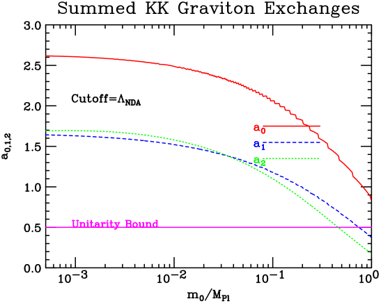
Figure 2: We plot ${\rm Re}~{}a_{0,1,2}$ as functions of $m_{0}/m_{Pl}$ as computed at $\sqrt{s}=\Lambda_{\rm NDA}$ and summing over all KK graviton resonances with mass below $\Lambda_{\rm NDA}$, but without including Higgs or radion exchanges.

We see that $W_{L}^{+}W_{L}^{-}\to W_{L}^{+}W_{L}^{-}$ scattering violates unitarity if $\Lambda_{\rm NDA}$ is employed as the cutoff. A more appropriate cutoff is determined numerically by requiring $|{\rm Re}~{}a_{0,1,2}|<1/2$ for $\sqrt{s}=\overline{\Lambda}$ after summing over KK resonances with mass below $\overline{\Lambda}$.

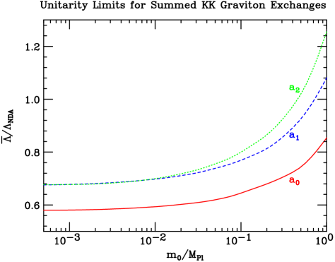
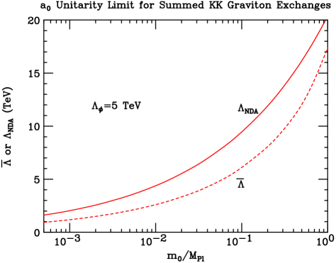
Figure 3: In the left hand plot, we give $\overline{\Lambda}/\Lambda_{\rm NDA}$ as a function of $m_{0}/m_{Pl}$, where $\overline{\Lambda}$ is the largest $\sqrt{s}$ for which $W_{L}^{+}W_{L}^{-}\to W_{L}^{+}W_{L}^{-}$ scattering is unitary after including KK graviton exchanges with mass up to $\overline{\Lambda}$, but before including Higgs and radion exchanges. Results are shown for the $J=0$, 1 and 2 partial waves. With increasing $\sqrt{s}$ unitarity is always violated earliest in the $J=0$ partial wave, implying that $J=0$ yields the lowest $\overline{\Lambda}$. The right hand plot shows the individual absolute values of $\overline{\Lambda}(J=0)$ and $\Lambda_{\rm NDA}$ for the case of $\Lambda_{\phi}=5~{}{\rm TeV}$; $\overline{\Lambda}/\Lambda_{\rm NDA}$ is independent of $\Lambda_{\phi}$

In the left-hand plot of Fig. 3, we display the ratio $\overline{\Lambda}/\Lambda_{\rm NDA}$ as a function of $m_{0}/m_{Pl}$, where $\overline{\Lambda}$ is the largest $\sqrt{s}$ for which $W_{L}^{+}W_{L}^{-}\to W_{L}^{+}W_{L}^{-}$ scattering is unitary when computed including only the KK graviton exchanges. Results are shown for $J=0$, 1, and 2. As a function of $\sqrt{s}$, the $J=0$ partial wave is always the first to violate unitarity and gives the lowest value of $\overline{\Lambda}$. As discussed in the introduction, we adopt the conservative approach of defining $\overline{\Lambda}$ to be the $J=0$ value. We will cut off our sums over KK exchanges when the KK mass reaches this $J=0$ value. We see that the $\overline{\Lambda}$ so defined is typically a significant fraction of $\Lambda_{\rm NDA}$, but never as large as $\Lambda_{\rm NDA}$. Still, it is quite interesting that the unitarity consistency limit $\overline{\Lambda}$ tracks the ’naive’ $\Lambda_{\rm NDA}$ estimate fairly well as $m_{0}/m_{Pl}$ changes over a wide range of values. (A very rough ’derivation’ of this result appears in our brief Appendix on approximate derivations.) The right-hand plot of Fig. 3 shows the actual values of $\overline{\Lambda}$ and $\Lambda_{\rm NDA}$ as functions of $m_{0}/m_{Pl}$ for the case of $\Lambda_{\phi}=5~{}{\rm TeV}$. Note that for larger $m_{0}/m_{Pl}$ they substantially exceed the input inverse coupling scale $\Lambda_{\phi}$, whereas for smaller $m_{0}/m_{Pl}$ they are both substantially below $\Lambda_{\phi}$. In other words, using either $\overline{\Lambda}$ or $\Lambda_{\rm NDA}$, one concludes that $\Lambda_{\phi}$, and equally $\widehat{\Lambda}_{W}$, are themselves not appropriate estimators for the maximum scale of validity of the model.

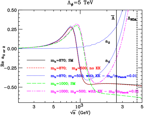
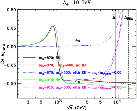
Figure 4: For $\Lambda_{\phi}=5~{}{\rm TeV}$ — left ($\Lambda_{\phi}=10~{}{\rm TeV}$ — right), we plot ${\rm Re}~{}a_{0}$ as a function of $\sqrt{s}$ for five cases: 1) solid (black) $m_{h}=870~{}{\rm GeV}$, SM contributions only ($\gamma=0$); 2) short dashes (red) $m_{h}=870~{}{\rm GeV}$, with an unmixed radion of mass $m_{\phi}=500~{}{\rm GeV}$ included, but no KK gravitons (we do not show the very narrow $\phi$ resonance); 3) dots (blue) as in 2), but including the sum over KK gravitons taking $m_{0}/m_{Pl}=0.01$ ($m_{0}/m_{Pl}=0.05$) — ${\rm Re}~{}a_{2}$ is also shown for this case; 4) long dashes (green) $m_{h}=1000~{}{\rm GeV}$ ($915~{}{\rm GeV}$), with an unmixed radion of mass $m_{\phi}=500~{}{\rm GeV}$, but no KK gravitons); 5) as in 4), but including the sum over KK gravitons taking $m_{0}/m_{Pl}=0.01$ ($m_{0}/m_{Pl}=0.05$). The $\overline{\Lambda}$ and $\Lambda_{\rm NDA}$ values for $m_{0}/m_{Pl}=0.01$ ($m_{0}/m_{Pl}=0.05$) are indicated by vertical lines.

It is worth noticing that the results obtained here can also be understood in terms of the strategy developed in Giudice:1998ck , where the discrete summation over KK gravitons is replaced by an integration over a continuous mass distribution when $m_{0}/m_{Pl}\ll 1$. In that limit, our results for the (relatively unimportant) $s$-channel contributions can be reproduced adopting the method of Giudice:1998ck . However, it should be emphasized that for moderate values of $m_{0}/m_{Pl}$ the discrete summation employed here is a more accurate procedure.

Let us now examine how the presence of a heavy Higgs boson affects $W_{L}^{+}W_{L}^{-}\to W_{L}^{+}W_{L}^{-}$ unitarity, both before and after inclusion of the exchanges of KK gravitons with mass below $\overline{\Lambda}$ (where $\overline{\Lambda}$ is the $J=0$ cutoff shown in Fig.3). In the left-hand plot of Fig. 4 we give ${\rm Re}~{}a_{0}$ as a function of $\sqrt{s}$ for the case of $\Lambda_{\phi}=5~{}{\rm TeV}$ for two different $m_{h}$ values and with and without radion and/or KK gravitons included. In the case where we include only the SM contributions for $m_{h}=870~{}{\rm GeV}$, the figure shows that ${\rm Re}~{}a_{0}$ asymptotes to a negative value very close to $-1/2$, implying that $m_{h}=870~{}{\rm GeV}$ is very near the largest value of $m_{h}$ for which unitarity is satisfied in $W_{L}^{+}W_{L}^{-}\to W_{L}^{+}W_{L}^{-}$ scattering in the SM context. If we add in just the radion contributions (for $m_{\phi}=500~{}{\rm GeV}$  – the $\phi$ resonance is very narrow and is not shown), then a sharp-eyed reader will see (red dashes) that ${\rm Re}~{}a_{0}$ is a bit more negative at the highest $\sqrt{s}$ plotted, implying earlier violation of unitarity. However, if we now include the full set of KK gravitons, which enter with an increasingly positive contribution, taking $m_{0}/m_{Pl}=0.01$ (dotted blue curve) one is far from violating unitarity due to ${\rm Re}~{}a_{0}<-1/2$ for $\sqrt{s}$ values above $m_{h}=870~{}{\rm GeV}$; instead, the positive KK graviton contributions, which cure the unitarity problem at negative ${\rm Re}~{}a_{0}$ for $\sqrt{s}$ above $m_{h}$, cause unitarity to be violated at large $\sqrt{s}$, but above $\overline{\Lambda}$, as ${\rm Re}~{}a_{0}$ passes through $+1/2$. In fact, in the case of a heavy Higgs boson we see that ${\rm Re}~{}a_{2}$ actually violates unitarity earlier than does ${\rm Re}~{}a_{0}$. However, even using ${\rm Re}~{}a_{2}$ as the criterion, unitarity is first violated for $\sqrt{s}$ values above the $\overline{\Lambda}$ value appropriate to the $m_{0}/m_{Pl}=0.01$ value being considered, but still below $\Lambda_{\rm NDA}$. In fact, it is very generally the case that unitarity is not violated at $\sqrt{s}=\overline{\Lambda}$ (which is typically a sizable fraction of $\Lambda_{\rm NDA}$) no matter how small we take $m_{0}/m_{Pl}$. However, as we shall see, unitarity can be violated in the vicinity of $\sqrt{s}\sim m_{h}$ if $m_{h}$ is large and $m_{0}/m_{Pl}$ is sufficiently small.

Looking again at the left plot of Fig. 4, we observe that if $m_{h}$ is increased to $1000~{}{\rm GeV}$, the purely SM plus radion contributions (long green dashes) show strong unitarity violation at large $\sqrt{s}$ due to ${\rm Re}~{}a_{0}<-1/2$. However, if we include the KK gravitons (long dashes and two shorter dashes in magenta), the negative ${\rm Re}~{}a_{0}$ unitarity violation disappears and unitarity is instead violated at higher $\sqrt{s}$. Thus, it is the KK gravitons that can easily control whether or not unitarity is violated for $\sqrt{s}<\overline{\Lambda}$ for a given value of $m_{h}$.

As discussed earlier, $\Lambda_{\phi}=5~{}{\rm TeV}$ is actually too low a value for consistency with Tevatron limits at $m_{0}/m_{Pl}=0.01$. Thus, in the right hand plot of Fig. 4 we show ${\rm Re}~{}a_{0}$ and ${\rm Re}~{}a_{2}$ for the case of $\Lambda_{\phi}=10~{}{\rm TeV}$ and $m_{0}/m_{Pl}=0.05$, a parameter set that is allowed by Tevatron KK limits. The heavier Higgs mass is chosen to be $915~{}{\rm GeV}$ in this case. The plot shows that $m_{h}=915~{}{\rm GeV}$ is just barely consistent with unitarity near ${\rm Re}~{}a_{0}=-1/2$ when KK gravitons are included. If $\Lambda_{\phi}$ is increased further, keeping $m_{0}/m_{Pl}=0.05$ fixed, the largest $m_{h}$ consistent with avoiding unitarity violation at ${\rm Re}~{}a_{0}=-1/2$ will decrease towards the SM value of $m_{h}=870~{}{\rm GeV}$.

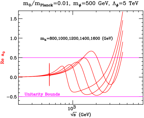
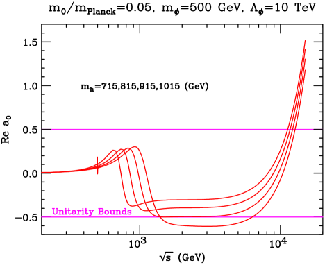
Figure 5: We plot ${\rm Re}~{}a_{0}$ as a function of $\sqrt{s}$ taking $m_{0}/m_{Pl}=0.01$ and $\Lambda_{\phi}=5~{}{\rm TeV}$ (left) or $m_{0}/m_{Pl}=0.05$ and $\Lambda_{\phi}=10~{}{\rm TeV}$ (right) for various Higgs masses. The curves terminate at $\sqrt{s}=\Lambda_{\rm NDA}$ as evaluated for a given $m_{0}/m_{Pl}$.

In Fig. 5 we display more clearly variations with $m_{h}$. The left plot shows that if $\Lambda_{\phi}=5~{}{\rm TeV}$ and $m_{0}/m_{Pl}=0.01$, the positive KK graviton contributions guarantee that ${\rm Re}~{}a_{0}$ never falls below $-1/2$ for any Higgs mass. In fact, one can increase $m_{h}$ to as high as $1400~{}{\rm GeV}$, at which point unitarity violation occurs near $\sqrt{s}=m_{h}$ at ${\rm Re}~{}a_{0}=+1/2$. The right plot of Fig. 5 contrasts this with results for $\Lambda_{\phi}=10~{}{\rm TeV}$ and $m_{0}/m_{Pl}=0.05$, a case consistent with Tevatron limits on the lightest KK resonance. For this case, the maximum Higgs mass allowed by unitarity is $m_{h}=915~{}{\rm GeV}$ and is determined by unitarity violation at ${\rm Re}~{}a_{0}=-1/2$.

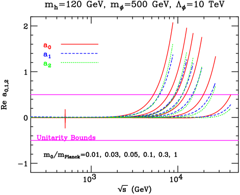
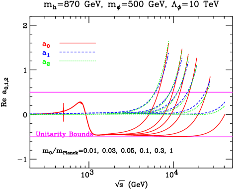
Figure 6: We plot ${\rm Re}~{}a_{0,1,2}$ as functions of $\sqrt{s}$ for $m_{h}=120~{}{\rm GeV}$ and $m_{h}=870~{}{\rm GeV}$, taking $m_{\phi}=500~{}{\rm GeV}$ and $\Lambda_{\phi}=10~{}{\rm TeV}$, and for the $m_{0}/m_{Pl}$ values indicated on the plot. Curves of a given type become higher as one moves to lower $m_{0}/m_{Pl}$ values. We have included all KK resonances with $m_{n}<\overline{\Lambda}$ (at all $\sqrt{s}$ values). Each curve terminates at $\sqrt{s}=\Lambda_{\rm NDA}$, where $\Lambda_{\rm NDA}$ at a given $m_{0}/m_{Pl}$ is as plotted earlier in Fig. 3. The value of $\sqrt{s}$ at which a given curve crosses above ${\rm Re}~{}a_{0}=+1/2$ is always slightly above the $\overline{\Lambda}$ (plotted in Fig. 3) value for the given $m_{0}/m_{Pl}$.

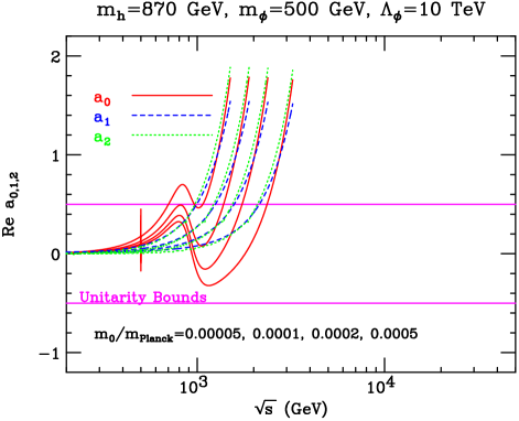
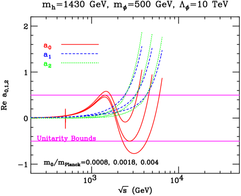
Figure 7: We plot ${\rm Re}~{}a_{0,1,2}$ as functions of $\sqrt{s}$ for $m_{h}=870~{}{\rm GeV}$ and $m_{h}=1430~{}{\rm GeV}$, taking $m_{\phi}=500~{}{\rm GeV}$ and $\Lambda_{\phi}=10~{}{\rm TeV}$, and for the $m_{0}/m_{Pl}$ values indicated on the plot. Otherwise, as in Fig. 6.

Thus, the Higgs plus vector boson exchange contributions have a large affect on the behavior for ${\rm Re}~{}a_{0}$ (whereas the radion exchange contributions are typically quite small in comparison). Let us consider further cases of $m_{h}$ and $m_{0}/m_{Pl}$ at fixed $m_{\phi}=500~{}{\rm GeV}$, taking $\Lambda_{\phi}=10~{}{\rm TeV}$ so as to indicate the influence of the KK resonance tower for an $\Lambda_{\phi}$ choice that for some $m_{0}/m_{Pl}$ values can be consistent with the Tevatron limits summarized earlier. We first consider $m_{h}=120~{}{\rm GeV}$ and $m_{h}=870~{}{\rm GeV}$. Fig. 6 shows the behavior of the real parts of the $a_{0,1,2}$ partial waves as a function of $\sqrt{s}$ for a series of $m_{0}/m_{Pl}$ values. For $m_{h}=120~{}{\rm GeV}$, the behavior of the amplitudes for $\sqrt{s}>200~{}{\rm GeV}$ is almost the same as in the absence of the Higgs and radion aside from the (very narrow) radion resonance peak. This is to be contrasted with the case of $m_{h}=870~{}{\rm GeV}$, for which one observes a (very broad) Higgs resonance in ${\rm Re}~{}a_{0}$, followed by a strong rise (depending on $m_{0}/m_{Pl}$) due to KK graviton exchanges. (For $J=1$ and 2 there is no resonance structure associated with the Higgs or radion since scalars do not contribute to $a_{1,2}$ in the s-channel.) As we have already noted, in the vicinity of the possible unitarity violation at negative $a_{0}$ from the SM plus radion contributions, the KK graviton exchanges give a possibly very relevant positive contribution to ${\rm Re}~{}a_{0}$.

A further plot for $m_{h}=870~{}{\rm GeV}$ and $\Lambda_{\phi}=10~{}{\rm TeV}$, but focusing on much smaller values of $m_{0}/m_{Pl}$, appears as the left-hand plot of Fig. 7. Note that for the very small value of $m_{0}/m_{Pl}=0.0001$, unitarity is only just satisfied for $\sqrt{s}\sim m_{h}$ and that ${\rm Re}~{}a_{0}$ exceeds $+1/2$ near $\sqrt{s}\sim m_{h}$ for $m_{0}/m_{Pl}<0.0001$. This is a general feature in the case of a heavy Higgs; there is always a lower bound on $m_{0}/m_{Pl}$ coming purely from unitarity. The right-hand plot of Fig. 7 shows how high we can push the mass of the Higgs boson without violating unitarity. For $m_{h}=1430~{}{\rm GeV}$, we are just barely consistent with the unitarity limit $|{\rm Re}~{}a_{0}|\leq 1/2$ (until large $\sqrt{s}\mathrel{\raise 1.29167pt\hbox{$>$\kern-7.5pt\lower 4.30554pt\hbox{$\sim$}}}\overline{\Lambda}$) if $m_{0}/m_{Pl}=0.0018$ (and $\Lambda_{\phi}=10~{}{\rm TeV}$). Any lower value of $m_{0}/m_{Pl}$ leads to ${\rm Re}~{}a_{0}>+1/2$ at $\sqrt{s}\sim m_{h}$ and any higher value leads to an excursion to ${\rm Re}~{}a_{0}<-1/2$ at higher $\sqrt{s}$ values (but still below $\overline{\Lambda}$). As discussed earlier, there are no limits of which we are aware on the $m_{0}/m_{Pl}$ values considered in Fig. 7 coming from direct production of KK gravitons. For such values, the KK gravitons would have very small masses. An analysis is needed.

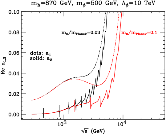
Figure 8: We plot ${\rm Re}~{}a_{1,2}$ for $m_{h}=870~{}{\rm GeV}$, $m_{\phi}=500~{}{\rm GeV}$ and $\Lambda_{\phi}=10~{}{\rm TeV}$ as functions of $\sqrt{s}$ for the $m_{0}/m_{Pl}$ values indicated on the plot. These are the same curves as the corresponding ones in Fig. 6, but plotted on an expanded scale so as to reveal the KK graviton resonances.

In order to actually see the graviton excitations in $a_{2}$ requires a much finer scale for the plot. We illustrate for the case of $m_{h}=870~{}{\rm GeV}$ and $\Lambda_{\phi}=10~{}{\rm TeV}$ in Fig. 8. The small KK resonance structures are apparent. As seen from the figure, the resonant graviton (spin 2) behavior is present only for $a_{2}$: no KK resonances appear in $a_{1}$.  The $a_{2}$ KK resonance peaks are suppressed by the partial $WW$ width to total width ratio. We have not attempted to determine if the resonances could actually be seen in $W_{L}^{+}W_{L}^{-}\to W_{L}^{+}W_{L}^{-}$ scattering at the LHC or a future ILC. However, it is important to note that other authors Davoudiasl:2000wi have shown that the resonance masses, cross sections and possibly widths can be measured in Drell-Yan production for instance at the LHC and in many different modes at a future ILC.

$\Lambda_{\phi}(~{}{\rm TeV})$	$5$	$10$	$20$	$40$
Absolute maximum Higgs mass
$m_{h}^{\rm max}(~{}{\rm GeV})$	1435	1430	1430	1430
required $m_{0}/m_{Pl}$	$1.32\times 10^{-2}$	$1.8\times 10^{-3}$	$2.3\times 10^{-4}$	$2.9\times 10^{-5}$
associated $m_{1}(~{}{\rm GeV})$	103.2	28.2	7.2	1.8
$m_{0}/m_{Pl}=0.005$: Tevatron limit: $m_{1}>??$
$m_{h}^{\rm max}(~{}{\rm GeV})$	1300	930	920	905
associated $m_{1}(~{}{\rm GeV})$	39	78	156	313
$m_{0}/m_{Pl}=0.01$: Tevatron limit: $m_{1}>240~{}{\rm GeV}$
$m_{h}^{\rm max}(~{}{\rm GeV})$	1405	930	910	895
associated $m_{1}(~{}{\rm GeV})$	78	156	313	626
$m_{0}/m_{Pl}=0.05$: Tevatron limit: $m_{1}>700~{}{\rm GeV}$
$m_{h}^{\rm max}(~{}{\rm GeV})$	930	915	900	885
associated $m_{1}(~{}{\rm GeV})$	391	782	1564	3129
$m_{0}/m_{Pl}=0.1$: Tevatron limit: $m_{1}>865~{}{\rm GeV}$
$m_{h}^{\rm max}(~{}{\rm GeV})$	920	910	893	883
associated $m_{1}(~{}{\rm GeV})$	782	1564	3128	6257

Table 2: Unitarity limits on $m_{h}$ for various $\Lambda_{\phi}$ and $m_{0}/m_{Pl}$ values.

In Table 2, we summarize the primary implications of our results by showing a number of limits on $m_{h}$ for the choices of $\Lambda_{\phi}=5$, 10, 20 and $40~{}{\rm TeV}$. The first block gives the very largest $m_{h}$ that can be achieved, $m_{h}^{\rm max}$, without violating unitarity in $W_{L}^{+}W_{L}^{-}\to W_{L}^{+}W_{L}^{-}$ scattering, along with the associated $m_{0}/m_{Pl}$ value and mass $m_{1}$ of the lightest KK graviton. Unfortunately, no Tevatron limits have been given for the associated very small $m_{0}/m_{Pl}$ values. Even if they end up being experimentally excluded, it is still interesting from a theoretical perspective that in the RS model unitarity can be satisfied for all $\sqrt{s}$ values below the $\overline{\Lambda}$ cutoff of the theory for a Higgs boson mass substantially higher than the usual $870~{}{\rm GeV}$ value applicable in the SM context. One finds that $m_{h}^{\rm max}$ is typically of order $1.4~{}{\rm TeV}$ if one chooses the optimal value for $m_{0}/m_{Pl}$. (A rough derivation of the value of $m_{h}^{\rm max}$ and associated optimal $m_{0}/m_{Pl}$ is given in the brief Appendix.) It is also noteworthy that the required values of $m_{0}/m_{Pl}$ are quite consistent with model expectations.

Table 2 also gives the $m_{h}^{\rm max}$ value achievable for the four $\Lambda_{\phi}$ cases listed above for various fixed $m_{0}/m_{Pl}$. Also given are the associated $m_{1}$ values and the Tevatron direct production limit when available. For some of the cases that are clearly consistent with Tevatron limits, unitarity is satisfied for $m_{h}$ values as high as $\sim 915~{}{\rm GeV}$.

Finally, we have seen that for a heavy enough Higgs boson mass, there will be a value of $m_{0}/m_{Pl}$ below which unitarity will be violated due to ${\rm Re}~{}a_{0}>+1/2$ for $\sqrt{s}\sim m_{h}$. Even for the relatively large value of $m_{h}\sim 870~{}{\rm GeV}$, the boundary value of $m_{0}/m_{Pl}$ for $\Lambda_{\phi}=10~{}{\rm TeV}$ is already very small, $m_{0}/m_{Pl}\sim 0.0001$, and this boundary value decreases rapidly as $m_{h}$ is decreased. Such small values are not favored in typical models and might also eventually be ruled out by an appropriate analysis of Tevatron data designed to exclude narrow KK resonances at very low mass.

V Parameter Determination from Experiment

In this section we summarize how our results might be applicable when future LHC data becomes available. As we have already noted, existing constraints are important in assessing the relevant range of parameters to which we should apply our results.

If the RS model is nature’s choice, then the LHC and/or ILC can potentially discover one or more graviton KK states. Their masses, cross sections and widths will provide a lot of information, and, as we shall discuss below, can strongly constrain the model. We will focus on the means for determining $m_{0}/m_{Pl}$ and $\Lambda_{\phi}$. (Given these, a determination of the cutoff $\overline{\Lambda}$ is possible.) To do so, it is sufficient to determine $m_{1}$ and its coupling to SM particles, which, see Eq. (3), is proportional to $1/\widehat{\Lambda}_{W}=\sqrt{3}/\Lambda_{\phi}$. If $m_{1}$ and $\Lambda_{\phi}$ are known, then it is possible to determine $m_{0}/m_{Pl}$ using Eq. (12).

If the graviton mass is known, then a measurement of the graviton width is one possible way to determine $\Lambda_{\phi}$. This was illustrated [after including phase space and non-asymptotic terms in Eq. (13)] in Fig. 1 for a selection of possible graviton masses in the range potentially observable at the LHC and/or ILC. Note that if the observed graviton is light, $m_{G}\mathrel{\raise 1.29167pt\hbox{$<$\kern-7.5pt\lower 4.30554pt\hbox{$\sim$}}}200~{}{\rm GeV}$, or $\Lambda_{\phi}$ is large, the graviton width(s) are very small compared to expected resolutions and cannot be used to extract $\Lambda_{\phi}$ — only a lower bound on $\Lambda_{\phi}$ could be extracted. Once, the mass and width are known, $m_{0}/m_{Pl}$ can be determined from Eq. (14) if we know which excitation level $n$ the KK resonance corresponds to.

If resolving the graviton resonance shape or determining the excitation index proves problematical, we should consider whether the absolute magnitude of the cross section for graviton production is a useful input. Consider first $e^{+}e^{-}\to G_{n}\to\mu^{+}\mu^{-}$. It is easy to demonstrate that the peak cross section at $s=m_{n}^{2}$ depends only on $m_{n}$ and not separately on $\Lambda_{\phi}$. Only if one can measure the shape of the cross section in the vicinity of the peak can one obtain the width and thereby determine $\Lambda_{\phi}$. However, as discussed above and shown in Fig. 1, for a large section of parameter space where $\Lambda_{\phi}$ is moderate in size and $m_{0}/m_{Pl}$ is in the preferred range of $\sim 0.01$, the graviton width will be much less than a GeV and a) a very fine scan will be needed to even find the graviton and b) sufficiently fine scan steps may not be possible to actually map out the shape of the excitation. It is easier to extract $\Lambda_{\phi}$ at fixed $m_{n}$ from the hadron collider cross section in some given final state, which cross section is proportional to $1/\Lambda_{\phi}^{2}$ at fixed $m_{n}$. Useful plots for $n=1$ appear in Allanach:2002gn (see their Figs. 1, 6–8 and 10–11). For $m_{0}/m_{Pl}=0.01$ (0.05), the $\gamma\gamma$ final state provides a highly accurate determination of $m_{1}$ and 20% accuracy or better for $\sigma(pp\to G_{1}){\rm BR}(G_{1}\to\gamma\gamma)$ for $m_{G}<1500~{}{\rm GeV}$ ($<3000~{}{\rm GeV}$).

Thus, for a wide range of parameters we will be able to determine both $\Lambda_{\phi}$ and $m_{0}/m_{Pl}$ with reasonable accuracy once LHC data is available. Given the measured values, we will be able to determine the maximum Higgs mass for which unitarity remains valid for all $\sqrt{s}$ below the cutoff $\overline{\Lambda}$. This might be useful if the Higgs boson turns out to be significantly heavier than the SM limit derived from unitarity, and therefore not easily seen as a clear resonance structure. Alternatively, if we find a Higgs boson and measure its mass, we will be able to determine a fairly precise value for the energy at which unitarity is violated and graviton interactions at the loop level start to become strong. This scale can be larger than $\overline{\Lambda}$ if $m_{h}$ is large and would be the scale at which additional new physics must enter.

VI Summary and Conclusions

We have discussed perturbative unitarity for $W_{L}^{+}W_{L}^{-}\to W_{L}^{+}W_{L}^{-}$ within the Randall-Sundrum theory with two 3-branes and shown that the exchange of massive 4D Kaluza-Klein gravitons leads to amplitudes growing linearly with the CM energy squared. We have found that the gravitational contributions cause a violation of unitarity for $\sqrt{s}$ below the natural cutoff of the theory, $\Lambda_{\rm NDA}$, as estimated using naive dimensional analysis. We have denoted by $\overline{\Lambda}$ the maximum $\sqrt{s}$ such that unitarity is still obeyed when summing graviton exchange contributions for gravitons with mass below $\overline{\Lambda}$. Although $\overline{\Lambda}<\Lambda_{\rm NDA}$, there is a rough tracking of $\overline{\Lambda}$ and $\Lambda_{\rm NDA}$ in that the ratio $\overline{\Lambda}/\Lambda_{\rm NDA}$ ranges from $\sim 0.6$ for small $m_{0}/m_{Pl}$ to $\sim 0.85$ at $m_{0}/m_{Pl}=1$, where $m_{0}$ is the curvature of the RS metric and $m_{Pl}$ is the usual 4d reduced Planck mass. This means that for a wide range of $m_{0}/m_{Pl}$ the two criteria are roughly in agreement as to the maximum energy scale for which the RS model will be a valid effective theory.

As we have shown, the KK resonance exchanges substantially modify constraints from unitarity and these modifications can have very important experimental implications. To determine these implications, consistent with the above discussion we sum over all KK gravitons with mass below $\overline{\Lambda}$, regardless of the $\sqrt{s}$ being considered. First, it is important to note that the two basic RS model parameters $\Lambda_{\phi}$ ($\Lambda_{\phi}^{-1}$ sets the strength of the couplings of matter fields to KK resonances) and $m_{0}/m_{Pl}$ can be extracted from experiment, especially LHC observations of the first KK excitation. If the Higgs mass has also been measured, then the maximum $\sqrt{s}$ for which $W_{L}^{+}W_{L}^{-}\to W_{L}^{+}W_{L}^{-}$ scattering obeys unitarity in the RS model can be determined from the results of this paper. For modest $m_{h}$, this $\sqrt{s}$ lies below $\Lambda_{\rm NDA}$, but above $\overline{\Lambda}$. More significantly, however, we have seen that values of the Higgs mass much larger (up to $1.435~{}{\rm TeV}$ in the sample case of $\Lambda_{\phi}=5~{}{\rm TeV}$) than the usual $m_{h}\sim 870~{}{\rm GeV}$ SM limit can be consistent with unitarity in $W_{L}^{+}W_{L}^{-}\to W_{L}^{+}W_{L}^{-}$ scattering if the $m_{0}/m_{Pl}$ parameter is chosen below some (typically small for large $\Lambda_{\phi}$) value. This happens by virtue of the fact that in the $\sqrt{s}\mathrel{\raise 1.29167pt\hbox{$>$\kern-7.5pt\lower 4.30554pt\hbox{$\sim$}}}m_{h}$ region, where ${\rm Re}~{}a_{0}$ can fall below $-1/2$ in the SM context when $m_{h}$ is large, the KK graviton exchanges enter with a positive sign and for small enough $m_{0}/m_{Pl}$ there are enough contributing KK exchanges that ${\rm Re}~{}a_{0}$ remains above $-1/2$. In such a case, unitarity is typically first violated by ${\rm Re}~{}a_{1}$ rising above $+1/2$ at a $\sqrt{s}$ value somewhat above $\overline{\Lambda}$. In addition, there is always a lower bound on $m_{0}/m_{Pl}$ coming from the requirement that ${\rm Re}~{}a_{0}$ not exceed $+1/2$ near the $\sqrt{s}\sim m_{h}$ resonance peak. For $m_{h}\leq 870~{}{\rm GeV}$, and quoting results for $\Lambda_{\phi}=10~{}{\rm TeV}$, the $m_{0}/m_{Pl}$ lower bound is very small (${\rm min}[m_{0}/m_{Pl}]\leq 0.0001$) and not particularly consistent with model expectations. However, as $m_{h}$ increases towards $1.43~{}{\rm TeV}$ the lower bound on $m_{0}/m_{Pl}$ increases rapidly, until it reaches a reasonably model-friendly value of $m_{0}/m_{Pl}\sim 0.0018$ at $m_{h}\sim 1.43~{}{\rm TeV}$. Experimental constraints hint that a value as low as $\Lambda_{\phi}=10~{}{\rm TeV}$ could be excluded when $m_{0}/m_{Pl}$ is small by a targeted analysis of Tevatron data; but currently there are no constraints in this $m_{0}/m_{Pl}$ region. For values of $m_{0}/m_{Pl}$ that are clearly consistent with current Tevatron limits we can only raise $m_{h}$ to $\sim 930~{}{\rm GeV}$ before violating unitarity in $W_{L}^{+}W_{L}^{-}\to W_{L}^{+}W_{L}^{-}$ scattering.

Still stronger constraints from unitarity per se can be obtained if one considers the full set of coupled channels ($WW$, $ZZ$, $hh$, …). The complete approach would undoubtedly result in a somewhat smaller value of $\overline{\Lambda}$ at a given $m_{0}/m_{Pl}$. We have chosen to adopt a somewhat conservative approach by focusing on $W_{L}W_{L}\to W_{L}W_{L}$ scattering, which is the most experimentally observable of the channels that will display unitarity violation at large energies.

In discussing unitarity issues for $W_{L}^{+}W_{L}^{-}\to W_{L}^{+}W_{L}^{-}$, we should note that it is not necessary to consider the effects of the scalar field(s) that are responsible for stabilizing the inter-brane separation at the classical level. While these fields too will have scalar excitations, the fields are normally chosen to be singlets under the SM gauge groups (sample models include those of Refs. Goldberger:1999wh ; Grzadkowski:2003fx ), and will thus have no direct couplings to the $W_{L}W_{L}$ channel. Their effects through mixing with the Higgs and radion can be neglected.

As a final remark, we note that it would be interesting to analyze unitarity constraints from KK graviton exchanges in other theories with extra dimensions, such as the many models with flat extra dimensions. We expect that the inclusion of the KK graviton modes would significantly modify the constraints from unitarity that are already known to arise from other types of KK excitations. For example, in universal extra dimension models it is known that the KK gauge boson excitations can cause unitarity violation if too many are included Chivukula:2003kq . Inclusion of the KK graviton excitations could modify the situation.

Acknowledgments

The authors thank Janusz Rosiek for his interest at the beginning of this project. B.G. thanks the CERN Theory Group for warm hospitality during the period part of this work was performed. This work is supported in part by the Ministry of Science and Higher Education (Poland) in years 2004-6 and 2006-8 as research projects 1 P03B 078 26 and N202 176 31/3844, respectively, by EU Marie Curie Research Training Network HEPTOOLS, under contract MRTN-CT-2006-035505, by the U.S. Department of Energy grant No. DE-FG03-91ER40674, and by NSF International Collaboration Grant No. 0218130. B.G. acknowledges the support of the European Community under MTKD-CT-2005-029466 Project. JFG thanks the Aspen Center for Physics where a portion of this work was performed. JFG also thanks H.-C. Cheng, J. Lykken, B. McElrath and J. Terning for helpful conversations.

APPENDIX: Rough derivations of some key results.

We first give a rough derivation of why it is that $\overline{\Lambda}$ tracks $\Lambda_{\rm NDA}$ and of the approximate numerical relation between them. We first recall that the spacing between KK states is, from Eq. (12), roughly $\Delta m=\pi(m_{0}/m_{Pl}){\widehat{\Lambda}_{W}\over\sqrt{2}}$. From Eq. (10), at $\sqrt{s}=\overline{\Lambda}$ we approximate the contribution to $a_{0}$ of each KK state as $a_{0}^{G}\sim{12\over 384\pi\widehat{\Lambda}_{W}^{2}}\overline{\Lambda}^{2}$, where we used $11+12\log(m_{G}^{2}/\overline{\Lambda}^{2})\sim-12$ (which we have checked is fairly accurate as an average for all KK states with mass below $\Lambda_{\rm NDA}$, nearly independent of $m_{0}/m_{Pl}$) and neglected all other terms. The number of contributing KK states is roughly given by $N_{G}\sim{\overline{\Lambda}\over\Delta m}$. At the unitarity limit we have $a_{0}={1\over 2}\sim a_{0}^{G}N_{G}$. Using this equation and inputing the relation (5) between $\widehat{\Lambda}_{W}$ and $\Lambda_{\rm NDA}$ yields $\overline{\Lambda}={\Lambda_{\rm NDA}\over\pi^{1/3}}\sim 0.7\Lambda_{\rm NDA}$, a result that is remarkably close to that obtained via the complete calculation.

Second, we wish to estimate the value, $m_{h}^{\rm max}\sim 1.43~{}{\rm TeV}$, of the largest Higgs mass allowed, and why it is that this maximum is more or less independent of $m_{0}/m_{Pl}$. We first note that in the extremal situation being considered it turns out that unitarity is violated at ${\rm Re}~{}a_{0}=-1/2$ at a $\sqrt{s}$ value quite close to $\overline{\Lambda}$. One can check this in the sample case presented in the right-hand plot of Fig. 7, where the $m_{0}/m_{Pl}=0.0018$ curve touches ${\rm Re}~{}a_{0}=-1/2$ at $\sqrt{s}=3~{}{\rm TeV}$ as compared to $\overline{\Lambda}\sim\Lambda_{\rm NDA}/\pi^{1/3}\sim 4.8~{}{\rm TeV}/\pi^{1/3}\sim 3.3~{}{\rm TeV}$. Thus, for our estimate we consider $\sqrt{s}=\overline{\Lambda}$ and, once again, we use $11+12\log(m_{G}^{2}/\overline{\Lambda}^{2})\sim-12$ on average and sum over $N_{G}\sim{\overline{\Lambda}\over\Delta m}$ KK states to obtain the net KK contribution of $a_{0}^{KK}=+1/2$ (independent of $m_{0}/m_{Pl}$), as employed in deriving $\overline{\Lambda}$ above. We now add in the asymptotic contribution of the Higgs boson for $\overline{\Lambda}\gg m_{h}$ as given in Eq. (10) of $a_{0}^{h}=-{1\over 8\pi}{m_{h}^{2}\over v^{2}}$. Setting $a_{0}^{KK}+a_{0}^{h}=-1/2$ gives $m_{h}\sim 1.23~{}{\rm TeV}$, more or less independent of $m_{0}/m_{Pl}$.

The above derivation makes it clear that the $\overline{\Lambda}$ for obtaining $m_{h}^{\rm max}$ in the extremal situation is $\overline{\Lambda}\sim 3.3~{}{\rm TeV}$, more or less independent of $m_{0}/m_{Pl}$. Now, given that $\overline{\Lambda}\sim\Lambda_{\rm NDA}/\pi^{1/3}$ and using Eq. (5) with $\widehat{\Lambda}_{W}=\Lambda_{\phi}/\sqrt{3}$, one obtains $m_{0}/m_{Pl}\sim(1.2~{}{\rm TeV}/\Lambda_{\phi})^{3}$ yielding values of $m_{0}/m_{Pl}\sim 1.38\times 10^{-2}$, $1.69\times 10^{-3}$, $2.16\times 10^{-4}$ and $2.70\times 10^{-5}$ at $\Lambda_{\phi}=5~{}{\rm TeV}$, $10~{}{\rm TeV}$, $20~{}{\rm TeV}$ and $40~{}{\rm TeV}$, respectively. These compare well with the values in the top box of Table 2.

References

- (1) L. Randall and R. Sundrum, Phys. Rev. Lett. 83 (1999) 3370 [arXiv:hep-ph/9905221]; Phys. Rev. Lett. 83 (1999) 4690 [arXiv:hep-th/9906064].
- (2) D. Dominici, B. Grzadkowski, J. F. Gunion and M. Toharia, Nucl. Phys. B 671, 243 (2003) [arXiv:hep-ph/0206192]; Acta Phys. Polon. B 33, 2507 (2002) [arXiv:hep-ph/0206197].
- (3) H. Davoudiasl, J. L. Hewett and T. G. Rizzo, Phys. Rev. Lett. 84, 2080 (2000) [arXiv:hep-ph/9909255].
- (4) A. Manohar and H. Georgi, Nucl. Phys. B 234, 189 (1984). Z. Chacko, M. A. Luty and E. Ponton, JHEP 0007, 036 (2000) [arXiv:hep-ph/9909248].
- (5) T. Han and S. Willenbrock, Phys. Lett. B 616, 215 (2005) [arXiv:hep-ph/0404182].
- (6) G. F. Giudice, R. Rattazzi and J. D. Wells, Nucl. Phys. B 595, 250 (2001) [arXiv:hep-ph/0002178].
- (7) Presented at the XXIX International Conference of Theoretical Physics ”Matter To The Deepest: Recent Developments In Physics of Fundamental Interactions”, Ustron, 8-14 September 2005, Poland., B. Grzadkowski and J. Gunion, Acta Phys. Polon. B 36, 3513 (2005).
- (8) W. D. Goldberger and M. B. Wise, Phys. Rev. D 60, 107505 (1999) [arXiv:hep-ph/9907218]; Phys. Rev. Lett. 83, 4922 (1999) [arXiv:hep-ph/9907447].
- (9) B. Grzadkowski and J. F. Gunion, Phys. Rev. D 68, 055002 (2003) [arXiv:hep-ph/0304241].
- (10) T. Han, G. D. Kribs and B. McElrath, Phys. Rev. D 64, 076003 (2001) [arXiv:hep-ph/0104074].
- (11) D. Choudhury, S. R. Choudhury, A. Gupta and N. Mahajan, J. Phys. G 28, 1191 (2002) [arXiv:hep-ph/0104143]; U. Mahanta, arXiv:hep-ph/0004128.
- (12) B. W. Lee, C. Quigg and H. B. Thacker, Phys. Rev. D 16, 1519 (1977).
- (13) Carsten Magass, presentation on behalf of the D0 collaboration at DPF-2006, Honolulu, Hawaii.
- (14) H. Davoudiasl, J. L. Hewett and T. G. Rizzo, Phys. Rev. D 63, 075004 (2001) [arXiv:hep-ph/0006041].
- (15) C. Csaki, M. L. Graesser and G. D. Kribs, Phys. Rev. D 63, 065002 (2001) [arXiv:hep-th/0008151].
- (16) G. F. Giudice, R. Rattazzi and J. D. Wells, Nucl. Phys. B 544, 3 (1999) [arXiv:hep-ph/9811291]. G. F. Giudice and A. Strumia, Nucl. Phys. B 663, 377 (2003) [arXiv:hep-ph/0301232]. G. F. Giudice, T. Plehn and A. Strumia, Nucl. Phys. B 706, 455 (2005) [arXiv:hep-ph/0408320].
- (17) D. Dicus and S. Willenbrock, Phys. Lett. B 609, 372 (2005) [arXiv:hep-ph/0409316].
- (18) B. C. Allanach, K. Odagiri, M. J. Palmer, M. A. Parker, A. Sabetfakhri and B. R. Webber, JHEP 0212, 039 (2002) [arXiv:hep-ph/0211205].
- (19) R. S. Chivukula, D. A. Dicus, H. J. He and S. Nandi, Phys. Lett. B 562, 109 (2003) [arXiv:hep-ph/0302263].