Simulations of Cold Electroweak Baryogenesis: Finite time quenches

Abstract:

The electroweak symmetry breaking transition may supply the appropriate out-of-equilibrium conditions for baryogenesis if it is triggered sufficiently fast. This can happen at the end of low-scale inflation, prompting baryogenesis to occur during tachyonic preheating of the Universe, when the potential energy of the inflaton is transfered into Standard Model particles. With the proper amount of CP-violation present, the observed baryon number asymmetry can be reproduced. Within this framework of Cold Electroweak Baryogenesis, we study the dependence of the generated baryon asymmetry on the speed of the quenching transition. We find that there is a separation between “fast” and “slow” quenches, which can be used to put bounds on the allowed Higgs-inflaton coupling. We also clarify the strong Higgs mass dependence of the asymmetry reported in a companion paper [1].

1 Introduction

The possibility of generating the observed baryon asymmetry at the electroweak phase transition dates back just over twenty years [2]. The Standard Model provides baryon number violating processes as well as CP-violation and potentially departure from thermal equilibrium. The task at hand is to discover a scenario in which these ingredients come together and generate the correct amplitude of the baryon asymmetry.

Cold Electroweak Baryogenesis was proposed as an alternative to Electroweak Baryogenesis at a bubble wall in a first order phase transition [3, 4, 5]. In the Minimal Standard Model such a transition is ruled out by bounds on the Higgs mass [6, 7, 8], and Cold Electroweak Baryogenesis relies on an out-of-equilibrium symmetry breaking transition triggered by the evolution of an inflaton field.

Inflation is supported by measurements of the CMB [9] and although the precise origin of the accelerated expansion has not been confirmed, models based on a scalar field rolling in a suitable potential can successfully reproduce observational signals. The energy scale of inflation is constrained by observations, but is ususally guided by expectations of physics beyond the Standard Model. In Cold Electroweak Baryogenesis, we apply a minimal extension to the Standard Model, a single inflaton, and assume that the energy scale of inflation is the Electroweak scale. Although this does not discard the possibility of further physics at higher energies, it allows for a self-contained description of baryogenesis. This because a period of electroweak-scale inflation will reduce the impact from whatever came before.

In section 2 we will introduce the relevant details of Cold Electroweak Baryogenesis. Tachyonic preheating with varying quench times is studied in section 3, with no CP-violation, where we observe the behaviour of CP-even observables. These results are then used in section 4, where we add CP-violation and compare the full simulation results to linear treatments based on the CP-even observables, as in [1]. We interpret the quench-time and mass dependence in terms of the winding around zeros of the Higgs field. Our conclusions are in section 5.

2 Cold Electroweak Baryogenesis

A number of conditions are to be met for Cold Electroweak Baryogenesis to be successful:

• A period of inflation has to take place that ends at sufficiently low energy, such that the reheating temperature is well below the electroweak scale. Then baryon number changing processes (sphaleron transitions) cannot wash out a previously generated asymmetry. Such low scale inflation can be made to agree with observational constraints, with some allowance for parameter tuning [10, 5, 11].

• Baryon number violation has to be effective while the system is out of equilibrium. The finite-temperature transition is a crossover rather than a phase transition in the Minimal Standard Model, [6, 7, 8], and hence the system stays close to equilibrium. The phase transition can however be first-order in supersymmetric models with an enlarged Higgs sector (see for instance [12]).

  We pursue here a different route. Out-of-equilibrium conditions can be introduced by triggering electroweak symmetry breaking through a coupling of the Higgs field to a rolling inflaton at or after the end of inflation. This results in a tachyonic instabiliy, which in turn can result in change of baryon number [3, 4, 5, 13, 14, 1].

• Although the gauge fields come out of equilibrium, an asymmetry is only created in the presence of CP-violation, the strength of which will determine the magnitude of the baryon asymmetry. The quark sector of the Minimal Standard Model seems unlikely to provide the required CP-violation [15, 16, 17, 18, 19]. The lepton sector has not been studied in similar detail. Here, as in [14, 1], we use only a simple CP-violating interaction composed of Higgs and gauge fields and consider it as representing the generic case.

A simple implementation of the scenario is obtained by adding effective CP violation to the SU(2)-Higgs sector of the SM, with action (we use the metric $(-+++)$)

$$S=-\int d^{3}{\bf x}\,dt\bigg{[}\frac{1}{2g^{2}}\mbox{Tr}\,F^{\mu\nu}F_{\mu\nu}+(D^{\mu}\phi)^{\dagger}D_{\mu}\phi+\epsilon+\mu_{\rm eff}^{2}\phi^{\dagger}\phi+\lambda(\phi^{\dagger}\phi)^{2}+\kappa\,\phi^{\dagger}\phi\,\mbox{Tr}\,F^{\mu\nu}\tilde{F}_{\mu\nu}\bigg{]},$$

The effective mass $\mu_{\rm eff}$ is supposed to depend on time, e.g. due to the coupling to an inflaton field $\sigma$,

$$\mu_{\rm eff}^{2}=\mu^{2}-\lambda_{\sigma\phi}\sigma^{2},$$ (1)

with a potential to appropriately generate low-scale inflation. In ‘inverted hybrid inflation’ models [20, 5, 11], $\sigma$ is very small during inflation as it rolls away from the origin. After inflation has ended it becomes substantial such that $\mu_{\rm eff}^{2}$ flips sign when $\sigma^{2}=\mu^{2}/\lambda_{\sigma\phi}$. Much later $\sigma$ and $\phi$ settle near their vacuum values and the eigenmodes and eigenvalues of the inflaton-Higgs mixing mass matrix determine the masses and other properties of the ensuing spinless particles [11].

The speed of the transition may be characterized by

$$u=\left.\frac{\sqrt{2}}{m_{H}^{3}}\,\frac{d\mu_{\rm eff}^{2}}{dt}\right|_{\mu_{\rm eff}^{2}=0}.$$ (2)

where we used the Higgs mass to set the scale. In [11] we assumed that viable baryogenesis would require a sufficiently fast quench $|u|\gtrsim 0.15$. For very fast quenches, the system is expected to be very much out-of-equilibrium, and in the limit of infinitely slow quenches, the system should stay in equilibrium throughout the symmetry breaking transition. One issue is to identify a transition between “fast” and “slow” transitions. This will allow us to constrain $\lambda_{\sigma\phi}$ and/or the shape of the inflaton potential around the time of symmetry breaking. Note that in the particular implementation of [11], inflation ends long before electroweak symmetry breaking, so that there is some freedom to tune the inflaton speed to accommodate a fast quench.

Setting aside the inflaton and the shape of its potential, we model the effective mass parameter by a linear form

$$\mu_{\rm eff}^{2}(t)= \mu^{2}\left(1-\frac{2t}{t_{Q}}\right), 0<t<t_{Q},$$ (3)

$$\mu_{\rm eff}^{2}(t)= -\mu^{2}, t>t_{Q}.$$ (4)

with $t_{Q}$ introduced as the quench time. In this model the Higgs v.e.v. and mass are given by the usual formulas $v^{2}=\mu^{2}/\lambda$ and $m_{H}^{2}=2\mu^{2}$, and $\epsilon=\mu^{4}/4\lambda$ is chosen to set the energy density of the vacuum to zero. Furthermore

$$|u|=\frac{1}{\mu t_{Q}}=\frac{\sqrt{2}}{m_{H}t_{Q}}.$$ (5)

For $|u|=0.15$, we find $m_{H}t_{Q}\approx 9$.

The baryon asymmetry now depends on three parameters

• The quench time $t_{Q}$.

• The strength of CP-violation, encoded in the coefficient of the CP-violating term, which we write in terms of a dimensionless $\delta_{\rm cp}$,

  $$\kappa=\frac{3\,\delta{\rm cp}}{16\pi^{2}m_{W}^{2}}.$$ (6)

  In [1] we found that the dependence on $\delta_{\rm cp}$ is linear at least for $\delta_{\rm cp}<1$. For example, at $m_{H}=2m_{W}$ this leads to

  $$\frac{n_{B}}{n_{\gamma}}=-(0.32\pm 0.04)\times 10^{-4}\,\delta_{\rm cp}.$$ (7)

• The mass of the Higgs boson, written as

  $$\left(\frac{m_{H}}{m_{W}}\right)^{2}=\frac{8\lambda}{g^{2}}.$$ (8)

  In [1], the mass dependence was seen to be quite complicated in the case of an instantaneous quench. We will confirm here, that the mass dependence is also present with non-instantaneous quenches; even the sign of the baryon asymmetry depends on $m_{H}$.

Shortly after $\mu_{\rm eff}^{2}$ has turned negative, the occupation numbers of the fields grow (faster than) exponentially with time. Initially, the non-linear terms in the equations of motion are not very large and it is reasonable to estimate $\langle\phi^{\dagger}\phi\rangle$ using a Gaussian approximation. The equation

$$\ddot{\phi}-\nabla^{2}\phi+\mu_{\rm eff}^{2}\phi=0,$$ (9)

where

$$\mu_{\rm eff}^{2}=-M^{3}(t-t_{c}),\quad t_{c}=t_{Q}/2,\quad M=(\mu t_{Q}/2)^{-1/3}\mu,$$ (10)

can be solved analytically, assuming the initial state at $t=0$ to be the free-field vacuum (see e.g. [21], for the instantaneous quench see [22]). Following the steps taken in [21], the (Fourier transform of the) equal-time two-point function is found to be given by

$$\langle\phi_{\bf k}\phi^{\dagger}_{\bf k}\rangle = |f_{k}(t)|^{2},$$ (11)

$$f_{k}(t) = C_{1k}Bi(\tau-k^{2}/M^{2})+C_{2k}Ai(\tau-k^{2}/M^{2}),\quad\tau=M(t-t_{c}),$$ (12)

$$C_{1k} = -\frac{\pi}{\sqrt{2\omega_{k}}}[Ai^{\prime}(-\omega_{k}^{2}/M^{2})+i\omega_{k}Ai(-\omega_{k}^{2}/M^{2})],\quad\omega_{k}=\sqrt{\mu^{2}+k^{2}},$$ (13)

$$C_{2k} = \frac{\pi}{\sqrt{2\omega_{k}}}[Bi^{\prime}(-\omega_{k}^{2}/M^{2})+i\omega_{k}Bi(-\omega_{k}^{2}/M^{2})].$$ (14)

Since the Airy functions behave for large $z$ like $Ai(z)\propto e^{(-2/3)z^{3}}$, $Bi(z)\propto e^{(2/3)z^{3}}$, it can be shown that occupation numbers of the unstable modes with $k\lesssim M\sqrt{\tau}$ grow very rapidly once $\tau>0$, and a classical approximation can be made for $\tau\gtrsim 2$ [21]. In fact, since quantum and classical evolution are identical in form, the classical evolution may already be started at time zero ($\tau=-Mt_{c}$), which is what we do in the numerical simulations (this is the analog of the “just the half” initial conditions in the case of the instantaneous quench [22]).

An important point to make is that energy is not conserved during a mass quench of the type (3), because $\mu_{\rm eff}$ depends explicitly on time. Differentiating the Hamiltonian corresponding to the action (2) and using the equations of motion one finds

$$\frac{dH}{dt}=\int d^{3}x\,\frac{d\mu_{\rm eff}^{2}}{dt}\,\phi^{\dagger}\phi.$$ (15)

Hence during the linear quench there is a change in energy density

$$\Delta\rho(t)=-\frac{2\mu^{2}}{t_{Q}}\int_{0}^{t}dt^{\prime}\,\langle\phi^{\dagger}\phi\rangle(t^{\prime})\approx-\frac{2\mu^{2}}{t_{Q}}\,4\int_{0}^{t}dt^{\prime}d^{3}{\bf k}|f_{k}(t^{\prime})|^{2},$$ (16)

where we made the Gaussian approximation in the last step (4 is the number of real components of the Higgs doublet). Evaluation of this analytic expression shows that the depletion in energy can be substantial.

In the case when the mass term comes from a coupling to an inflaton field (1), the energy extracted from the gauge-Higgs system is transferred into inflaton energy. Had we included the dynamics of the inflaton itself, this energy would not be lost but would come back through additional reheating as the inflaton oscillates and eventually decays. Including a dynamical inflaton does however complicate the system somewhat, since it implies unknown parameters such as $\lambda_{\sigma\phi}$ and other masses and couplings of a potential $V(\sigma,\phi)$.

We shall use the approximation (3) in the present work to bypass the complications of the additional degree of freedom, because it is easy to implement and solve analytically at early times, and because it can represent a source of mass quenching other than a coupling to an inflaton. We are therefore not bound to a specific model.

When calculating the final asymmetry, we will need to know the final reheating temperature. We will then specialise to the case of a Higgs-inflaton coupling, assume $m_{\sigma}>m_{W}$ and that all the initial energy is equipartitioned between the SM particles at a temperature $T_{\rm reh}<m_{W}$.

3 No CP violation

In order to understand the underlying gauge and Higgs dynamics, it is useful to study the evolution of various observables in absence of CP violation. The CP-violation can then, at least at early times, be thought of as a small perturbation on this background.

The numerical implementation is identical to the one introduced in [14, 1]. In short, the action (2) is discretised on a lattice, and the classical equations of motion solved in real time. This is done for a CP-symmetric ensemble of initial conditions, reproducing the Higgs field correlators of the vacuum state at $t=0$, when the Higgs potential is $V=\epsilon+\mu^{2}\phi^{\dagger}\phi$ in the Gaussian approximation. The initial gauge field is set by $A^{\mu}=0$ and we impose the Gauss constraint on the gauge momenta for a given random Higgs field background. Observables are averaged over the ensemble.

The observables of interest (in a periodic volume $L^{3}$) are the Higgs field averaged over the volume,

$$\overline{\phi^{2}}=\frac{1}{L^{3}}\int d^{3}x\,\phi^{\dagger}\phi=\frac{1}{L^{3}}\int d^{3}x\,\frac{1}{2}\mbox{Tr}\,\Phi^{\dagger}\Phi,\quad\Phi=(i\tau_{2}\phi^{*},\phi),$$ (17)

the volume-averaged magnetic field,

$$\overline{B^{2}}=\frac{1}{L^{3}}\int d^{3}x\,\mbox{Tr}\,F_{ij}F_{ij},$$ (18)

the distribution of Higgs winding number,

$$N_{\rm w}=\frac{1}{24\pi^{2}}\int d^{3}x\epsilon_{ijk}\mbox{Tr}\,U^{\dagger}\left(\partial_{i}U\right)U^{\dagger}\left(\partial_{j}U\right)U^{\dagger}\left(\partial_{k}U\right),\quad U=\frac{\Phi}{\sqrt{\frac{1}{2}\mbox{Tr}\,\Phi^{\dagger}\Phi}},$$ (19)

the width of the Chern-Simons number distribution

$$\Delta_{\rm cs}(t)=\langle[N_{\rm cs}(t)-N_{\rm cs}(0)]^{2}\rangle,\quad N_{\rm cs}(t)-N_{\rm cs}(0)=\int_{0}^{t}dt\int d^{3}x\,\frac{1}{16\pi^{2}}\mbox{Tr}\,F^{\mu\nu}\tilde{F}_{\mu\nu},$$ (20)

and its time derivative, the Chern-Simons number diffusion rate or susceptibility,

$$\Gamma=\frac{d\Delta(t)}{dt}.$$ (21)

In equilibrium, $\Gamma$ is the sphaleron rate.

The dynamics of a tachyonic electroweak phase transition has been studied in some detail in terms of these and related observables in [13, 23] (with an inflaton), in the limit of an instantaneous quench in [14, 24, 1], and in terms of suitably defined particle numbers in [25]. The above observables are all global quantities (integrals over space). Since $A^{\mu}=0$ initially, also $N_{\rm cs}(0)=0$. The Chern-Simons number and the winding number can be changed by an integer through a “large” gauge transformation, but $N_{\rm cs}-N_{\rm w}$ is gauge invariant. Classical vacuum configurations have $N_{\rm cs}-N_{\rm w}=0$, and are gauge equivalent to $N_{\rm cs}=N_{\rm w}=0$.

We now motivate the study of one other observable, the distribution of $\phi^{\dagger}\phi$ over the volume, in particular its magnitude near $\phi^{\dagger}\phi=0$. The study in [24] concentrated on local observables, such as Chern-Simons and winding-number densities, in an attempt to clarify how CP violation causes an asymmetry in the final Chern-Simons number. It was observed that the transition produced initially many centers with high winding-number density, dubbed ‘half-knots’ since their winding number in small balls is roughly $\pm 1/2$. They can only disappear or be created when the Higgs length $\sqrt{\phi^{\dagger}\phi}$ becomes zero in their center. This happens at early times because of the rapid growth of long distance modes, and then the number of half-knots rapidly diminishes, but when the volume-averaged Higgs length has grown substantially, $\overline{\phi^{2}}=\mathcal{O}(v^{2})$, such zeros have become rare. Subsequently the Higgs field ‘overshoots’ the minimum of its potential, rolls back and moves again towards zero, and when $\overline{\phi^{2}}$ goes through its first minimum, new zeros in the Higgs length occur, enabling the creation of new half-knots. In this way second, third, …, generation half-knots were observed [24] near the minima of the oscillating $\overline{\phi^{2}}$. Since the gauge field is initially very small, CP violation is ineffective in influencing the creation or annihilation of the first generation half-knots. However, by the time of the first minimum of $\overline{\phi^{2}}$, the gauge field has grown substantially, CP violation can be effective and may change the balance and cause an asymmetry in $\langle N_{\rm cs}\rangle$. Because of the importance of Higgs zeros, we shall in section 4.4 present results for the distribution of the local Higgs field length, a simple histogram of $\phi^{\dagger}(x)\phi(x)$ for various quench times.

We found in [1] that the asymmetry depends strongly on the Higgs mass. The extreme cases seem to be $m_{H}=2m_{W}\simeq 161$ GeV and $m_{H}=\sqrt{2}\,m_{W}\simeq 114$ GeV . In addition to the quench time dependence, we are interested in how this mass dependence comes about. Below, we will show plots for these two Higgs masses in parallel, to demonstrate the differences throughout. Since the physical Higgs masses, at least in the Minimal Standard Model are constrained to be within $114$ and $200$ GeV [8], both options are (marginally) allowed.

3.1 Higgs field

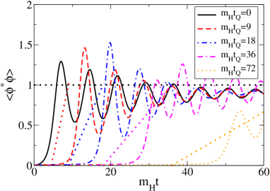
Figure 1: The normalized Higgs expectation value $2\langle\overline{\phi^{2}}\rangle/v^{2}$ vs time, for different quench times (full lines). Dotted lines show $v^{2}(t)/v^{2}$ correspondingly colour coded. Left: $m_{H}=2m_{W}$, right: $m_{H}=\sqrt{2}m_{W}$.

As the Higgs mass parameter changes from positive to negative, the naive Higgs expectation value goes from $0$ for $t<t_{Q}/2$, to $v^{2}(t)=-\mu_{\rm eff}^{2}(t)/\lambda$ up until $t=t_{Q}$, after which it stays at $v^{2}=\mu^{2}/\lambda$.

Figure 1 shows the evolution of the normalized Higgs average value $\langle 2\overline{\phi^{2}}\rangle/v^{2}$ (cf. (17)) for various quench times. Dotted lines show $v^{2}(t)/v^{2}$ for the different $t_{Q}$. For small quench times, the symmetry breaking time is determined by the time it takes for the dynamics to perform the rolling off the local maximum of the potential at $\phi=0$. For $m_{H}t_{Q}<36$, $v^{2}(t)$ reaches $v^{2}$ before $\langle 2\overline{\phi^{2}}(t)\rangle$ reaches $v^{2}(t)$. For larger quench times, $\langle 2\overline{\phi^{2}}(t)\rangle$ catches up with $v^{2}(t)$, and oscillates around it before settling around $v^{2}$. In the limit of infinite quench time one would expect it to follow $v^{2}(t)$ closely, except for finite-temperature corrections.

We notice that the amplitudes of the first maximum and minimum are quench-time dependent, and also mass dependent. Although the qualitative behaviour is the same, $m_{H}=\sqrt{2}m_{W}$ leads to a lower first Higgs minimum.

The evolution of the Higgs field determines the energy loss in (the first half of) Eq. (16) due to the time-dependent effective mass. We integrate the actual numerical $\langle\phi^{2}\rangle$ up to time $t_{Q}$ to find that for $t_{Q}=(0,9,13.5,18,36,72)$ Eq. (16) predicts

$$|\Delta\rho/\rho_{\rm initial}|\simeq~{}0,~{}0.06,~{}0.10,~{}0.19,~{}0.66,~{}0.84.$$ (22)

By directly calculating the energy, we find

$$|\Delta\rho/\rho_{\rm initial}|\simeq~{}0,~{}0.04,~{}0.08,~{}0.17,~{}0.67,~{}0.83.$$ (23)

Note that for the very slowest quenches, more than half the energy is lost. For these slow quenches, at $t=t_{Q}$ the field has already started its oscillation, and so the Gaussian approximation (the second half of Eq. (16)) does not apply. Integrating the actual field evolution reproduces the energy depletion.

3.2 Magnetic field

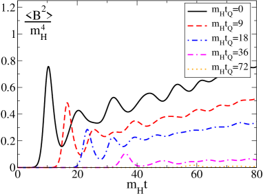
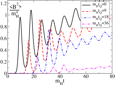
Figure 2: The evolution of the magnetic field $\overline{B^{2}}$ for different $t_{Q}$. $m_{H}=2\,m_{W}$ (left), $m_{H}=\sqrt{2}\,m_{W}$ (right).

As the Higgs field goes through its transition, energy is transfered to the gauge fields, the occupation numbers of which grow exponentially [25]. The gauge fields acquire energy very fast at first, and then slowly towards what will be an equipartitioned and thermalised final state, figure 2. This later transfer is quench-time dependent, faster quenches lead to a faster transfer of energy. To some extent, this decrease in energy transfer is due to the depletion of energy resulting from the time-dependent $\mu_{\rm eff}$, and the relative growth $\dot{B^{2}}/B^{2}$ is in fact similar for different quench times. The dependence on the Higgs mass is also interesting. For $m_{H}=\sqrt{2}\,m_{W}$ the transfer seems to be driven by the Higgs field oscillations, with the gauge field also oscillating even for rather late times. In particular the second maximum is much larger than for $m_{H}=2\,m_{W}$.

3.3 Chern-Simons diffusion

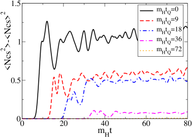
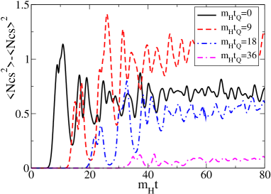
Figure 3: $\langle N_{\rm cs}^{2}\rangle$ for different quench times. $m_{H}=2\,m_{W}$ (left), $m_{H}=\sqrt{2}\,m_{W}$ (right).

In the absence of CP-violation, the ensemble average of the Chern-Simons number itself is zero, Chern-Simons number being CP-odd. In our setup, the ensemble is strictly CP-even, so $\langle N_{\rm cs}\rangle$ is also strictly zero.

We can also calculate the evolution of the width of the $N_{\rm cs}$ distribution, which will grow as a result of the preheating of the gauge fields, similar to the $B$-field. But also because of fluctuations at finite temperature (and out of equilibrium, at finite energy density) there is a non-zero diffusion rate of Chern-Simons number, $\Gamma(t)=d\Delta_{\rm cs}/dt$ (cf. (20)). The rate $\Gamma(t)$ enters in an estimate of the baryon asymmetry in section 4.

Figure 3 shows the evolution of $\Delta_{\rm cs}$ for various quench times. There is a rapid growth, which in some cases appears to be further driven by the Higgs field oscillations. Eventually $\Delta_{\rm cs}$ settles, in accordance with the fact that at the final emerging temperatures the equilibrium sphaleron rate is negligible. This is one of the central features of Cold Electroweak Baryogenesis, the generated asymmetry does not get further diluted by sphaleron transitions. Similar to the magnetic field, at least for $m_{H}=\sqrt{2}\,m_{W}$, the Chern-Simons number seems to be driven by the Higgs oscillations. However, whereas the growth of the magnetic field has a monotonic dependence on the quench rate, the diffusion rate appears to have a more complicated dependence.

4 Adding CP-violation

For small enough values of the CP-violation parameter $\delta_{\rm cp}$, it was seen in [1] that the baryon asymmetry is linear. The value of $\delta_{\rm cp}$ required to reproduce the observed asymmetry, is comfortably within this linear range. We shall keep $\delta_{\rm cp}=1$ throughout, the upper end of the range studied in [1], in order to maximise the generated numerical signal.

Because the CP-violation is small, we have the option to treat it as a perturbation on the CP-even background described in the previous section. Although we will include the CP-violating term completely in the dynamics below, we will first apply the early time approximations introduced in [26, 3, 13, 14] for the case of finite-time quenches.

4.1 Initial rise

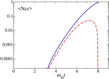
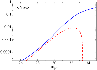
Figure 4: The initial rise, comparing the simulation (dashed, red) to Eq. (24) (full, black), for $m_{H}t_{Q}=0$ (left) and $36$ (right). Notice the logarithmic axis.

For very early times, only very long wavelength modes have large occupation numbers, both in the Higgs and gauge fields, since modes only gradually become unstable, starting with the zero mode at time $t_{Q}/2$. Treating the CP-violation as a perturbation to the CP-even evolution, and making a homogeneous approximation, we find for the average Chern-Simons number [22]

$$\langle N_{\rm cs}\rangle=\frac{\sqrt{2}\,\delta_{\rm cp}(Lm_{H})^{3}}{64\pi^{4}(1+c)^{2}}\,\frac{\langle\overline{B^{2}}\rangle}{m_{H}^{4}}\,\frac{\langle\overline{\phi^{2}}\rangle}{v^{2}/2}.$$ (24)

The values of $B^{2}(t)$ and $\phi^{2}(t)$ are taken from the simulations, section 3. The constant $c$ is extracted from the growth of the gauge field $\overline{B^{2}}(t)\propto e^{2ct}$. The linearisation assumes exponential growth of the Higgs and gauge fields. This description will have to break down at some fairly early time, when the back-reaction of gauge and Higgs non-linear self-interaction becomes important. Figure 4 shows the linear approximation compared to the full simulation for short and long quench times. The agreement is good during the initial exponential growth, but breaks down after about 5 and 10 units of $m_{H}t$ after $\mu_{\rm eff}^{2}$ has gone negative at $t=t_{Q}/2$, respectively for $t_{Q}=0$ and 36.

4.2 Thermodynamic treatment

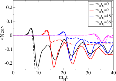
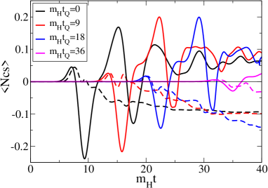
Figure 5: The average Chern-Simons number in the full simulations (full line) and from the thermodynamic treatment (dashed line). $m_{H}=2\,m_{W}$ (left), $\sqrt{2}\,m_{W}$ (right).

Beyond the linear approximation, we can apply methods from non-equilibrium thermodynamics [26, 3, 13, 14] to estimate the asymmetry.

One can interpret the CP-violating term as a chemical potential for Chern-Simons number (cf. (2,6)):

$$\int d^{4}x\,\kappa\phi^{\dagger}\phi\mbox{Tr}\,F\tilde{F}\leftrightarrow-\int dt\,\mu_{\rm ch}N_{\rm cs},\quad\mu_{\rm ch}(t)=\frac{3\delta_{\rm cp}}{m_{W}^{2}}\frac{d}{dt}\langle\overline{\phi^{2}}(t)\rangle.$$ (25)

Using the CP-even evolution of the diffusion rate Eq. (21) and the Higgs average Eq. (17), the average Chern-Simons number can then be estimated through

$$\langle N_{\rm cs}\rangle(t)=\frac{1}{T_{\rm eff}}\int_{0}^{t}dt^{\prime}\,\Gamma(t^{\prime})\mu_{\rm ch}(t^{\prime}),$$ (26)

where $T_{\rm eff}$ was interpreted in [3] as the effective temperature of the tachyonic modes. We will not elaborate here on such an interpretation, but merely observe that $T_{\rm eff}$ turns out to decrease roughly linearly with $t_{Q}$, and that $m_{H}=\sqrt{2}\,m_{W}$ gives much larger values, figure  6.

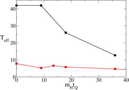
Figure 6: The effective temperature in units of $m_{H}$ as extracted from the thermodynamical treatment. Squares: $m_{H}=2\,m_{W}$, circles: $m_{H}=\sqrt{2}\,m_{W}$.

Figure 5 compares the result of Eq. (26) to the full simulation. $T_{\rm eff}$ is chosen to fit the first maximum of the full simulation. The approximation nicely reproduces the change of sign of the asymmetry produced by the back-reaction. At later times, the approximation again breaks down. We will see that this is precisely the time when the Higgs field acquires a net winding number [1], the dynamics of which can apparently not be described by a simple chemical potential with constant $T_{\rm eff}$. The effective temperatures as a function of $t_{Q}$ are shown in figure 6.

Notice in figure 5 that the sign of the asymmetry at later times $m_{H}t\sim 40$ has changed again to positive (the sign of $\delta_{\rm cp}$) in the case of mass ratio $\sqrt{2}$, which is not captured by the thermodynamic treatment. In principle the latter might do better, since the oscillations in $\mu_{\rm ch}(t)$ and $\Gamma(t)$ are correlated. In any case, replacing the diffusion rate by its time average [13]

$$\int_{0}^{t_{max}}dt^{\prime}\Gamma(t^{\prime})\mu_{\rm ch}(t^{\prime})~{}~{}\rightarrow\bar{\Gamma}\int_{0}^{t_{max}}dt^{\prime}\mu_{\rm ch}(t^{\prime})=\frac{3\delta_{\rm cp}\bar{\Gamma}v^{2}}{2m_{W}^{2}},$$ (27)

gives a sign of the asymmetry that is definitely equal to that of $\delta_{\rm cp}$, which may be wrong.

4.3 Full simulation

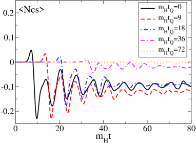
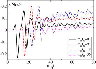
Figure 7: The evolution of Chern-Simons number in time, $m_{H}=2\,m_{W}$ (left), $m_{H}=\sqrt{2}\,m_{W}$ (right).

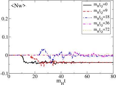
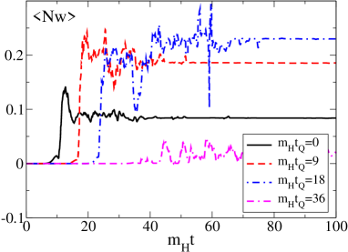
Figure 8: The evolution of winding number in time, $m_{H}=2\,m_{W}$ (left), $m_{H}=\sqrt{2}\,m_{W}$ (right).

In order to capture the full dependence on quench time and Higgs mass, we need to include the CP-violation completely in the dynamics. Figure 7 shows the average Chern-Simons number for various quench times. Figure 8 is the corresponding winding number. We notice that the mass dependence found in [1] is robust, and not a pathology of an instantaneous quench. For $m_{H}=2\,m_{W}$, the fastest quenches $m_{H}t_{Q}=0,9$ lead to an asymmetry of opposite sign to $\delta_{\rm cp}$. For slower quenches, the noise dominates and we can only conclude that the final asymmetriy is consistent with zero. In contrast, for $m_{H}=\sqrt{2}\,m_{W}$, the asymmetry has the same sign as $\delta_{\rm cp}$, and it is maximal for intermediate quench times $m_{H}t_{Q}=18$. Recall also the maximal boosting of $\Delta_{\rm cs}$ in section 3 was seen at these quench times. In both cases, for $m_{H}t_{Q}=36$ and larger the asymmetry appears to vanish. This is all compiled in figure 9 which shows the final asymmetry versus quench time.

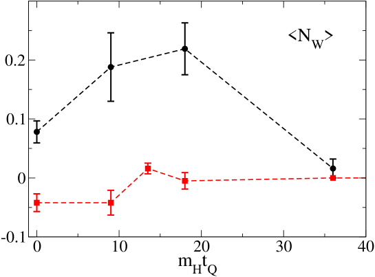
Figure 9: Final asymmetry vs. quench time for $m_{H}=2\,m_{W}$ (squares) and $\sqrt{2}\,m_{W}$ (circles).

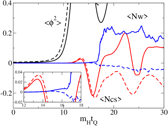
Figure 10: A close-up of the early evolution of $\langle\overline{\phi^{2}}\rangle$ (black), $\langle N_{\rm cs}\rangle$ (red) and $\langle N_{W}\rangle$ (blue). Full lines are $m_{H}=\sqrt{2}\,m_{W}$, dashed $m_{H}=2\,m_{W}$. The quench time $m_{H}t_{Q}=9$. The inset is a further amplification around the initial winding number bump.

4.4 Higgs field zeros

We have observed in earlier work [14, 24] that the final asymmetry in $\langle N_{\rm cs}\rangle$ can already be seen at earlier times in $\langle N_{\rm w}\rangle$, which may be expected from the fact that the temperature after the transition is low enough that sphaleron transitions are suppressed and the robustness of winding number under relatively small changes in the fields. The asymmetry in $\langle N_{\rm w}\rangle$ is induced by the CP violating terms in the equations of motion, which are very small during the first stages of the instability, as monitored roughly by $\overline{\phi^{2}}$ and $\overline{B^{2}}$. Somewhat later the asymmetry becomes visible in the initial rise and bouncing back of $\langle N_{\rm cs}\rangle$, and a little later also in $\langle N_{\rm w}\rangle$. The rise in $\langle N_{\rm w}\rangle$ is much smaller than in $\langle N_{\rm cs}\rangle$, presumably since $N_{\rm w}$ can only change when there are zeros in the Higgs field, which are exceptional by that time. Still somewhat later, around the time $\langle\overline{\phi^{2}}\rangle$ has its first minimum, $\langle N_{\rm w}\rangle$ has grown substantially, as new (second generation) zeros appear in the Higgs field.

This is illustrated in figure 10, which shows the evolution of $\langle N_{\rm cs}\rangle$, $\langle N_{\rm w}\rangle$ and $\langle\overline{\phi^{2}}\rangle$ at early times. At the time of the initial bump of $\langle N_{\rm cs}\rangle$ the winding asymmetry $\langle N_{\rm w}\rangle$ is still not visible, but a growth of a ‘bump’ is discernible by the time $\langle N_{\rm cs}\rangle$ has crossed zero and reached a negative maximum. When $\langle\overline{\phi^{2}}\rangle$ reaches its first minimum the asymmetry in $\langle N_{\rm w}\rangle$ grows much faster, which we interpret as being caused by the asymmetric creation of second generation winding centers, made possible by zeros in the Higgs lengths.

Figure 11: Histogram of $\phi^{2}(x)$ over the lattice for $m_{H}=2\,m_{W}$. Colours correspond to quench times $m_{H}t_{Q}=0$ (black), $9$ (red), $18$ (green) and $36$ (blue). The four graphs correspond to the first four minima of the Higgs oscillation in each case.

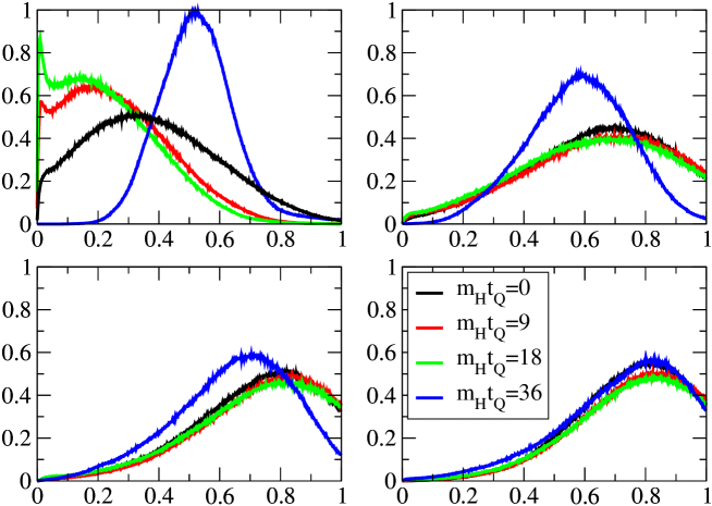
Figure 12: Histogram of $\phi^{2}(x)$ over the lattice for $m_{H}=\sqrt{2}\,m_{W}$. Colours correspond to quench times $m_{H}t_{Q}=0$ (black), $9$ (red), $18$ (green) and $36$ (blue). The four graphs correspond to the first four minima of the Higgs oscillation in each case.

To illustrate the presence or absence of zeros in the Higgs field we show histograms of $\phi^{2}(x)$ over the lattice for the first 4 minima of the Higgs oscillation, in figures 11 and 12. Figure 11 is for $m_{H}=2\,m_{W}$, and we see that although the average is away from zero (figure 1), there is still a tail stretching to zero, at least for the first two minima. These will provide nucleation points for winding. In figure 1, we also saw that for the smaller Higgs mass $m_{H}=\sqrt{2}\,m_{W}$, the Higgs minima were somewhat lower. It is remarkable, however how different the distributions in the first minimum look (figure 12). The proximity of the distribution bulk to zero (and the fact that $\phi^{2}(x)\geq 0$) results in points aggregating close to zero. Qualitatively, the density of zeros follows the same behaviour as a function of quench time as the final asymmetry of figure 9.

4.5 Kibble mechanism

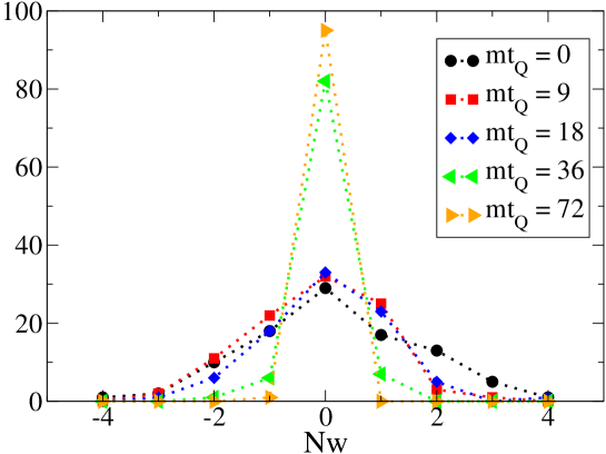
Figure 13: The final distribution of winding number for various $t_{Q}$. $m_{H}=2\,m_{W}$.

During a symmetry breaking transition, a net density of defects will form through the Kibble mechanism [27]. In the present case of $O(4)$ symmetry in 3+1 dimensions, these textures have integer winding number in the Higgs field, spread out over space. The density of gauged defects can be predicted in terms of the evolution of the correlation length of the system [28]. Numerical studies often consider thermal quenches with overdamped dynamics through the transition. In our case, we have an underdamped system with no explicit coupling to a thermal bath (higher-momentum modes do play the role of a bath). Still, we here illustrate “fast” and “slow” quenches in terms of the number of defects generated.

Figure 13 shows the distribution of final winding number over the ensemble. There is a qualitative difference between $m_{H}t_{Q}=0$, 9, 18 and $m_{H}t_{Q}=36$, 72. Also from this distribution we see that $m_{H}t_{Q}=18$ still belongs to the regime of ‘fast’ quenches, whereas $m_{H}t_{Q}=36$ is definitely in the ‘slow’ regime.

5 Conclusions

We have confirmed in a more realistic setting that including CP-violation in the SU(2)-Higgs equations leads to baryogenesis, when going through a tachyonic electroweak transition. The dependence on quench time is significant. Although our scan of quench time is not fine enough to give a precise characterisation of ‘fast’ and ‘slow’ quenches, we can say that $m_{H}t_{Q}\lesssim 20$ belongs to the first category, corresponding to

$$|u|=\left|\frac{d\mu_{\rm eff}^{2}(t)}{2\mu^{3}dt}\right|_{t=t_{Q}/2}\gtrsim 0.07.$$ (28)

This constrains a possible underlying Hybrid inflation model in terms of the Higgs-inflaton coupling $\lambda_{\sigma\phi}$, since $\mu_{\rm eff}^{2}(t)=\mu^{2}-\lambda_{\sigma\phi}\sigma^{2}$.

It is satisfying that the dramatic mass dependence seen in [1] is not a result of the instantaneous quench. It is, however, surprising that for $m_{H}=\sqrt{2}\,m_{W}$ the maximum asymmetry is not generated at the fastest quenches but for intermediate $t_{Q}$. Both the mass dependence and the quench time dependence can be put down to a coincidence of phases and frequencies of the Higgs and gauge oscillations. This is similar to the much simpler model in 1+1 dimensions studied in [22].

An important aspect of the transition is the occurrence of zeros in the Higgs field. CP-violation generates asymmetries in the Chern-Simons number density, which prompts the winding number density to move along as well. The full winding number change is however only realised once the second generation Higgs zeros appear. Although some settling of winding and Chern-Simons number can occur at later generations, we find that the asymmetry is established at the first Higgs minimum.

The quench time and the mass (through the Higgs self-coupling) influence the number of zeros, and so determine the magnitude of the asymmetry by allowing more half-knots to flip their winding number. The detailed dynamics are very complicated.

The expansion of the Universe is negligible at electroweak-scale temperatures, but reheating may proceed differently in the presence of all the other Standard Model fields and in particular an oscillating inflaton [23]. Still, because the final asymmetry is largely determined during the first couple of Higgs oscillations, we expect that the results presented here are reasonably close to the complete result.

The maximal asymmetry occurred in our simulation for $m_{H}=\sqrt{2}\,m_{W}$ and $m_{H}t_{Q}=18$. We can estimate the photon density by distributing the initial energy density over the Standard Model degrees of freedom, which gives:

$$\frac{n_{B}}{n_{\gamma}}=(0.20\pm 0.04)\times 10^{-3}\,\delta_{\rm cp}.$$ (29)

about three times the result at zero quench time [1]. This means that we require $\delta_{\rm cp}=3\times 10^{-6}$ or larger to reproduce the observed baryon asymmetry.

Acknowledgments

We thank Meindert van der Meulen and Denes Sexty for collaboration on related subjects and useful comments. A.T. is supported by PPARC Special Programme Grant “Classical Lattice Field Theory”. Part of this work was conducted on the COSMOS supercomputer, funded by HEFCE, PPARC and SGI, and on the SARA PC-cluster LISA. This work received support from FOM/NWO.

References

- [1] A. Tranberg and J. Smit, Simulations of cold electroweak baryogenesis: Dependence on higgs mass and strength of CP-violation, JHEP 08 (2006) 012, [hep-ph/0604263].
- [2] V. A. Kuzmin, V. A. Rubakov, and M. E. Shaposhnikov, On the anomalous electroweak baryon number nonconservation in the early universe, Phys. Lett. B155 (1985) 36.
- [3] J. García-Bellido, D. Y. Grigoriev, A. Kusenko, and M. E. Shaposhnikov, Non-equilibrium electroweak baryogenesis from preheating after inflation, Phys. Rev. D60 (1999) 123504, [hep-ph/9902449].
- [4] L. M. Krauss and M. Trodden, Baryogenesis below the electroweak scale, Phys. Rev. Lett. 83 (1999) 1502–1505, [hep-ph/9902420].
- [5] E. J. Copeland, D. Lyth, A. Rajantie, and M. Trodden, Hybrid inflation and baryogenesis at the TeV scale, Phys. Rev. D64 (2001) 043506, [hep-ph/0103231].
- [6] F. Csikor, Z. Fodor, and J. Heitger, Endpoint of the hot electroweak phase transition, Phys. Rev. Lett. 82 (1999) 21–24, [hep-ph/9809291].
- [7] K. Kajantie, M. Laine, K. Rummukainen, and M. E. Shaposhnikov, The electroweak phase transition: A non-perturbative analysis, Nucl. Phys. B466 (1996) 189–258, [hep-lat/9510020].
- [8] Particle Data Group Collaboration, S. Eidelman et. al., Review of particle physics, Phys. Lett. B592 (2004) 1.
- [9] D. N. Spergel et. al., Wilkinson microwave anisotropy probe (wmap) three year results: Implications for cosmology, astro-ph/0603449.
- [10] G. German, G. Ross, and S. Sarkar, Low-scale inflation, Nucl. Phys. B608 (2001) 423–450, [hep-ph/0103243].
- [11] B. van Tent, J. Smit, and A. Tranberg, Electroweak-scale inflation, inflaton-Higgs mixing and the scalar spectral index, JCAP (2004) [hep-ph/0404128].
- [12] M. Laine and K. Rummukainen, The MSSM electroweak phase transition on the lattice, Nucl. Phys. B535 (1998) 423–457, [hep-lat/9804019].
- [13] J. García-Bellido, M. García-Pérez, and A. González-Arroyo, Chern-Simons production during preheating in hybrid inflation models, Phys. Rev. D69 (2004) 023504, [hep-ph/0304285].
- [14] A. Tranberg and J. Smit, Baryon asymmetry from electroweak tachyonic preheating, JHEP 0311 (2003) 016, [hep-ph/0310342].
- [15] M. E. Shaposhnikov, Baryon asymmetry of the universe in standard electroweak theory, Nucl. Phys. B287 (1987) 757–775.
- [16] M. E. Shaposhnikov, Structure of the high temperature gauge ground state and electroweak production of the baryon asymmetry, Nucl. Phys. B299 (1988) 797.
- [17] M. B. Gavela, M. Lozano, J. Orloff, and O. Pène, Standard model CP violation and baryon asymmetry. Part 1: Zero temperature, Nucl. Phys. B430 (1994) 345–381, [hep-ph/9406288].
- [18] M. B. Gavela, P. Hernandez, J. Orloff, O. Pène, and C. Quimbay, Standard model CP violation and baryon asymmetry. Part 2: Finite temperature, Nucl. Phys. B430 (1994) 382–426, [hep-ph/9406289].
- [19] J. Smit, Effective CP violation in the standard model, JHEP 09 (2004) 067, [hep-ph/0407161].
- [20] D. H. Lyth and E. D. Stewart, More varieties of hybrid inflation, Phys. Rev. D54 (1996) 7186–7190, [hep-ph/9606412].
- [21] J. García-Bellido, M. García Perez, and A. González-Arroyo, Symmetry breaking and false vacuum decay after hybrid inflation, Phys. Rev. D67 (2003) 103501, [hep-ph/0208228].
- [22] J. Smit and A. Tranberg, Chern-Simons number asymmetry from CP violation at electroweak tachyonic preheating, JHEP 12 (2002) 020, [hep-ph/0211243].
- [23] A. Díaz-Gil, J. García-Bellido, M. García Pérez, and A. González-Arroyo, Magnetic field production after inflation, PoS LAT2005 (2005) 242, [hep-lat/0509094].
- [24] M. van der Meulen, D. Sexty, J. Smit, and A. Tranberg, Chern-Simons and winding number in a tachyonic electroweak transition, JHEP 02 (2006) 029, [hep-ph/0511080].
- [25] J.-I. Skullerud, J. Smit, and A. Tranberg, W and Higgs particle distributions during electroweak tachyonic preheating, JHEP 08 (2003) 045, [hep-ph/0307094].
- [26] S. Y. Khlebnikov and M. E. Shaposhnikov, The statistical theory of anomalous fermion number nonconservation, Nucl. Phys. B308 (1988) 885–912.
- [27] T. W. B. Kibble, Topology of cosmic domains and strings, J. Phys. A9 (1976) 1387–1398.
- [28] M. Hindmarsh and A. Rajantie, Defect formation and local gauge invariance, Phys. Rev. Lett. 85 (2000) 4660–4663, [cond-mat/0007361].