Gluon mass generation in the PT-BFM scheme

Abstract

In this article we study the general structure and special properties of the Schwinger-Dyson equation for the gluon propagator constructed with the pinch technique, together with the question of how to obtain infrared finite solutions, associated with the generation of an effective gluon mass. Exploiting the known all-order correspondence between the pinch technique and the background field method, we demonstrate that, contrary to the standard formulation, the non-perturbative gluon self-energy is transverse order-by-order in the dressed loop expansion, and separately for gluonic and ghost contributions. We next present a comprehensive review of several subtle issues relevant to the search of infrared finite solutions, paying particular attention to the role of the seagull graph in enforcing transversality, the necessity of introducing massless poles in the three-gluon vertex, and the incorporation of the correct renormalization group properties. In addition, we present a method for regulating the seagull-type contributions based on dimensional regularization; its applicability depends crucially on the asymptotic behavior of the solutions in the deep ultraviolet, and in particular on the anomalous dimension of the dynamically generated gluon mass. A linearized version of the truncated Schwinger-Dyson equation is derived, using a vertex that satisfies the required Ward identity and contains massless poles belonging to different Lorentz structures. The resulting integral equation is then solved numerically, the infrared and ultraviolet properties of the obtained solutions are examined in detail, and the allowed range for the effective gluon mass is determined. Various open questions and possible connections with different approaches in the literature are discussed.

I Introduction

The generation of mass gaps in QCD is one of the most fundamental problems in particle physics. In part the difficulty lies in the fact that the symmetries governing the QCD Lagrangian prohibit the appearance of mass terms for all fundamental degrees of freedom at tree-level and, provided that these symmetries are not violated through the procedure of regularization, this masslessness persists to all orders in perturbation theory. Thus, mass generation in QCD becomes an inherently non-perturbative problem, whose tackling requires the employment of rather sophisticated calculational tools and approximation schemes Marciano:su .

Whereas the generation of quark masses is intimately connected with the breaking of chiral symmetry Lane:1974he , it was argued long ago that the non-perturbative QCD dynamics lead to the generation of an effective gluon mass, while the local gauge invariance of the theory remains intact JMCKursu ; Cornwall:1979hz ; Parisi:1980jy ; Berg:1980gz ; Bhanot:1980fx ; Bernard:1981pg ; Smit:1974je . This gluon “mass” is not a directly measurable quantity, but must be related to other physical parameters such as the string tension, glueball masses, or the QCD vacuum energy Shifman:1978by , and furnishes, at least in principle, a regulator for all infrared (IR) divergences of QCD.

The concept of a dynamically generated gluon mass, its field theoretic realization, and a plethora of physical and technical issues associated with it, have been explored in great detail in a classic paper by Cornwall Cornwall:1982zr . One of the cornerstones in his analysis was the insistence on preserving, at every level of approximation, crucial properties such as gauge-invariance, gauge-independence, and invariance under the renormalization-group (RG). With this motivation, an effective gluon propagator, $\widehat{\Delta}_{\mu\nu}$, was derived through the systematic rearrangement of Feynman graphs, a procedure that is now known in the literature as the “pinch technique” (PT) Cornwall:1989gv ; Papavassiliou:1989zd ; Binosi:2002ft . The self-energy, $\widehat{\Pi}_{\mu\nu}$, of this propagator is gauge-independent and captures the leading logarithms of the theory, exactly as happens with the vacuum polarization in QED. The central result of  Cornwall:1982zr was that, when solving the Schwinger-Dyson (SD) equation governing the PT propagator, and under special assumptions for the form of the three-gluon vertex, one finds solutions that are free of the Landau singularity, and reach a finite value in the deep IR. These solutions may be successfully fitted by a massive propagator, with the crucial characteristic, encoded in the corresponding SD equation, that the mass employed is not “hard”, but depends non-trivially on the momentum transfer, vanishing sufficiently fast in the deep ultraviolet (UV). From the dimensionfull massive solutions one may define a dimensionless quantity, which constitutes the generalization in a non-Abelian context of the universal (process-independent) QED effective charge. The QCD effective charge so obtained displays asymptotic freedom in the UV, whereas in the IR it “freezes” at a finite value.

Various independent field theoretic studies Bernard:1982my ; Lavelle:1991ve ; Kondo:2001nq ; Bloch:2003yu ; Aguilar:2004sw ; Dudal:2004rx ; Sorella:2006ax , spanning over a quarter of a century, also corroborate some type of gluon mass generation. In addition, lattice computations Alexandrou:2000ja ; Bonnet:2000kw ; Sternbeck:2005tk reveal the onset of non-perturbative effects, which in principle can be modelled by means of effectively massive gluon propagators. It is important to emphasize that the massive gluon propagator derived in  Cornwall:1982zr describes successfully nucleon-nucleon scattering when inserted, rather heuristically, into the two-gluon exchange model Halzen:1992vd ; for additional phenomenological applications, see Mihara:2000wf . Furthermore, several theoretical studies based on a-priori very distinct approaches  Cornwall:1989gv ; Mattingly:1993ej ; Dokshitzer:1995qm ; vonSmekal:1997is ; Badalian:1999fq ; Aguilar:2002tc ; Brodsky:2002nb ; Baldicchi:2002qm ; Grunberg:1982fw ; Gies:2002af ; Shirkov:1997wi ; Gracey:2006dr ; Prosperi:2006hx support the notion of the “freezing” of the QCD running coupling in the deep IR (but do not agree, in general, on its actual value).

In recent years there has been significant progress in our understanding of the PT construction in general Binosi:2002ez , and the properties of the resulting effective Green’s functions in particular. The extension of the PT to all orders was carried out in Binosi:2002ft , and the known one- Denner:1994nn and two-loop Papavassiliou:1999az connection with the BFM  Dewitt:ub ; Abbott:1980hw was shown to persist to all orders. From the practical point of view the established connection permits the direct calculation with a set of concrete Feynman rules, and enables one to prove all-order results, exploiting the powerful formal machinery of the BFM. In what follows we will refer to the framework emerging from the synergy between PT and BFM as the “PT-BFM scheme”.

The aim of this article is threefold: First, we initiate a systematic treatment of the SD equations within the PT-BFM scheme, with particular emphasis on the manifestly gauge-invariant truncation it offers. Second, we discuss various field-theoretic issues relevant to the study of gluon mass generation in the context of SD equations in general. Third, we analyze in detail the SD equation obtained as the first non-trivial approximation in the aforementioned truncation scheme, and search for infrared finite solutions.

Regarding our first objective, let us point out that one of the most distinct features of the PT-BFM scheme is the special way in which the transversality of the background gluon self-energy $\widehat{\Pi}_{\mu\nu}$ is realized. In particular, the study of the non-perturbative, SD-type of equation obeyed by $\widehat{\Pi}_{\mu\nu}$ reveals that, by virtue of the Abelian-like Ward Identities (WI) satisfied by the vertices involved, the transversality is preserved without the inclusion of ghosts. Put in another way, gluonic and ghost contributions are separately transverse. In addition, transversality is enforced without mixing the orders in the usual “dressed-loop” expansion: the “one-loop-dressed” and “two-loop-dressed” sets of diagrams are independently transverse. This is to be contrasted to what happens in the usual gauge-fixing scheme of the covariant renormalizable gauges, where the inclusion of the ghost is crucial for the transversality already at the level of the one-loop perturbative calculation. This particular transversality property of the BFM self-energy is known at the level of the one-loop calculation Abbott:1980hw ; however, to the best of our knowledge, its all-order generalization presented in Sec. II appears for the first time in the literature. The importance of this property in the context of SD equation is that it allows for a meaningful first approximation: instead of the system of coupled equations involving gluon and ghost propagators, one may consider only the subset containing gluons, without compromising the crucial property of transversality. More generally, one can envisage a systematic dressed loop expansion, maintaining transversality manifest at every level of approximation.

Instrumental for some of the developments mentioned above has been a set of non-trivial identities Gambino:1999ai , relating the BFM $n$-point functions to the corresponding conventional $n$-point functions in the covariant renormalizable gauges, to all orders in perturbation theory. These identities, to be referred to as Background-Quantum identities (BQIs) Binosi:2002ez , are expected to play a fundamental role in addressing one of the most central issues in the context of the PT-BFM scheme, namely the actual construction of a new SD series. Specifically, as is known already from the two-loop analysis Papavassiliou:1999az , the PT-BFM gluon self-energy $\widehat{\Pi}_{\mu\nu}$ is expressed in terms of Feynman diagrams containing the conventional gluon self-energy ${\Pi}_{\mu\nu}$; this fact is generic, as the all-order diagrammatic representation of $\widehat{\Pi}_{\mu\nu}$ demonstrates (see Sec. II). Clearly, in order to arrive at a genuine SD equation for $\widehat{\Pi}_{\mu\nu}$, one must carry out the substitution ${\Pi}_{\mu\nu}\to\widehat{\Pi}_{\mu\nu}$ inside the loops. It is still an open question whether such a replacement can be implemented self-consistently to all orders; a preliminary view of how this might work out is presented in Sec. II.

Turning to the analysis of the SD equations and the search for infrared finite solutions, after setting up the appropriate theoretical stage in Sec. III, in the next two sections we eventually study a linearized version of the equation governing the PT propagator $\widehat{\Delta}_{\mu\nu}$, in the spirit of Cornwall:1982zr . Although several of the techniques developed there are adopted virtually unchanged in the present work, there are important theoretical and phenomenological differences, which we summarize below.

(i) The role of the ghosts: As has become clear from the detailed study of the correspondence between PT and BFM, the rearrangement of graphs (or sets of graphs) implemented by the PT generates dynamically the characteristic ghost sector of the BFM Binosi:2002ft . However, since the original one-loop derivation of the PT self-energy  Cornwall:1982zr the calculations were carried out in the context of the ghost-free light cone gauge, the distinction between gluonic and ghost contributions was not so obvious. As a result, in the heuristic derivation of the corresponding SD equation, all contributions were treated as gluonic. This is reflected in the fact that the coefficient multiplying the characteristic term $\ln(q^{2}+4m^{2}(q^{2}))$ appearing in the solutions (e.g. the standard RG logarithm supplemented with the non-perturbative mass) is precisely $b=11C_{A}/48\pi^{2}$, namely the coefficient of the one-loop QCD $\beta$ function. Instead, the PT-BFM correspondence reveals that the purely gluonic contributions is ${\tilde{b}}=10C_{A}/48\pi^{2}$. Needless to say, the point is not so much the minor numerical discrepancy in the coefficients multiplying the logs, but rather the possibility that the ghost dynamics may behave in a completely different way in the IR. Thus, whilst the ghosts will eventually furnish the missing $C_{A}/48\pi^{2}$ asymptotically, their IR contribution may deviate from the massive logarithm given above, inducing qualitative changes in the form of the full gluon self-energy. Reversing the argument, in order to actually obtain solutions of the type $b\ln(q^{2}+4m^{2}(q^{2}))$ from the coupled gluon-ghost system of SD equations, a very delicate interplay between gluons and ghosts must take place.

(ii) Form of the three-gluon vertex: It is well-known that in order to obtain dynamically generated masses one must allow for the presence of massless poles in the corresponding expression for the three-gluon vertex Jackiw:1973tr . The effective vertex used in the SD equation of Cornwall:1982zr was the bare three-gluon vertex obtained from the Lagrangian of the (non-renormalizable) massive gauge-invariant Yang-Mills model  KuniGoto ; Forshaw:1998tf ; it contains kinematic poles, whose dimensionality is partially compensated by the explicit appearance of a hard mass term in the numerator. Instead, we use a gauge-technique inspired Ansatz for the vertex Salam:1963sa , which also contains kinematic poles, but their dimensionality is saturated solely by appropriate combinations of the momenta involved, with no explicit reference to mass terms, thus being closer to what one might expect to obtain within QCD. We hasten to emphasize that our Ansatz for the vertex is completely phenomenological, and is not derived from any dynamical principle, other than the WI that it satisfies, nor does it exhaust the possible Lorentz structures. What we hope to obtain by resorting to such a simplified vertex is a manageable SD equation, that will allow us to study in detail the complicated interplay of the various components, and get a feel for the dependence of the solutions on the form of the vertex used.

(iii) Seagull regularization: As was explained in Cornwall:1982zr , the integral equation describing gluon mass generation is supplemented by a non-trivial constraint, expressing $\widehat{\Delta}^{-1}(0)$ in terms of (quadratically divergent) seagull-like contributions; after its regularization, this constraint will restrict severely the number of possible solutions. The phenomenological “glueball regularization” employed in Cornwall:1982zr was based on an elaborate connection between the seagull contributions, the massive Yang-Mills model, and the finite vacuum expectation value of a scalar field creating glueball states. Instead, the regulation we introduce in this work is based solely on dimensional regularization. In particular, the non-perturbative seagull contributions are regulated by subtracting from them the elementary integral $\int d^{4}k/k^{2}$, which vanishes in dimensional regularization. It turns out that this subtraction is sufficient to regulate the expression for $\widehat{\Delta}^{-1}(0)$, provided that the momentum-dependent mass vanishes “sufficiently fast” in the deep UV. In turn, this required asymptotic behavior restricts the values of the parameters appearing in the integral equation.

(iv)Type of solutions: For relatively moderate values of $\widehat{\Delta}^{-1}(0)$, which at the level of the integral equation is treated as an input, the type of solutions emerging may be fitted with great accuracy by means of a monotonically decreasing dynamical mass and a running coupling, exactly as advocated in Cornwall:1982zr . However, as one decreases $\widehat{\Delta}^{-1}(0)$ beyond a critical value, a new class of qualitatively different solutions begins to emerge. These solutions are also finite in the entire range of momentum, but they display a sharp increase in the deep IR, and the corresponding plateau-like range, associated with the “freezing”, becomes increasingly narrower.

The paper is organized as follows: In Sec. II we review the BT-BFM scheme, and the structure of the all-order gluon self-energy. In Sec. III we present some general considerations pertinent to the search for IR finite solutions, with particular emphasis on the role of transversality, the kinematic poles in the vertex employed, the restoration of the correct UV behavior at the level of the SD equation, and the regularization of the seagull terms. In Sec. IV we derive the linearized integral equation and discuss in detail several of its characteristics. Sec. V contains the numerical analysis, focusing particularly on the appearance of two types of solutions, as mentioned above. Finally, in Sec. VI we discuss connection of this work with other approaches in the literature, outline various possible future directions, and summarize our conclusions.

II The PT-BFM scheme

In this section we study the structure of the effective gluon self-energy obtained within the PT-BFM framework. In the first subsection we present a brief overview of the PT and its connection with the BFM. The discussion presented here is meant to serve as a brief reminder; for a more complete treatment the reader is referred to the extensive literature on the subject. In the second subsection we present the all-order diagrammatic structure of the gluon propagator. In the third subsection we first derive an elementary WI, valid in the ghost sector of the BFM, and then demonstrate that, to all orders, the contributions of gluonic and ghost loops to the effective gluon self-energy are separately transverse. Finally, in the last subsection we present a preliminary view of how the PT may eventually lead to a new SD series.

II.1 The connection between PT and BFM

The PT Cornwall:1982zr ; Cornwall:1989gv is a well-defined algorithm that exploits systematically the symmetries built into physical observables, such as $S$-matrix elements, in order to construct new, effective Green’s functions endowed with very special properties. Most importantly, they are independent of the gauge-fixing parameter, and satisfy naive (ghost-free, QED-like) WIs instead of the usual Slavnov-Taylor identities. The basic observation, which essentially defines the PT, is that there exists a fundamental cancellation between sets of diagrams with different kinematic properties, such as self-energies, vertices, and boxes. This cancellation is driven by the underlying BRST symmetry Becchi:1976nq , and is triggered when a very particular subset of the longitudinal momenta circulating inside vertex and box diagrams generate out of them (by “pinching” out internal lines) propagator-like terms. The latter are reassigned to conventional self-energy graphs, in order to give rise to the aforementioned effective Green’s functions.

The longitudinal momenta responsible for these diagrammatic rearrangements stem either (a) from the bare gluon propagators contained inside the various Feynman diagrams,

$$\Delta_{\mu\nu}^{[0]}(k)=-\frac{\displaystyle i}{\displaystyle k^{2}}\left[\ g_{\mu\nu}-(1-\xi)\frac{\displaystyle k_{\mu}k_{\nu}}{\displaystyle k^{2}}\right]\,,$$ (2.1)

and/or (b) from the “pinching part” $\Gamma^{{\rm P}}_{\alpha\mu\nu}(q,p_{1},p_{2})$ appearing in the characteristic decomposition of the bare three-gluon vertex $\Gamma^{eab}_{\alpha\mu\nu}=gf^{eab}\Gamma_{\alpha\mu\nu}$ into Cornwall:1982zr

$$\Gamma_{\alpha\mu\nu}(q,p_{1},p_{2}) = \Gamma^{{\rm F}}_{\alpha\mu\nu}(q,p_{1},p_{2})+\Gamma^{{\rm P}}_{\alpha\mu\nu}(q,p_{1},p_{2}),$$

$$\Gamma^{{\rm F}}_{\alpha\mu\nu}(q,p_{1},p_{2}) = (p_{1}-p_{2})_{\alpha}g_{\mu\nu}+2q_{\nu}g_{\alpha\mu}-2q_{\mu}g_{\alpha\nu},$$

$$\Gamma^{{\rm P}}_{\alpha\mu\nu}(q,p_{1},p_{2}) = p_{2\nu}g_{\alpha\mu}-p_{1\mu}g_{\alpha\nu}.$$ (2.2)

The case of the gluon self-energy is of particular interest. Defining the transverse projector

$${\rm P}_{\mu\nu}(q)=\ g_{\mu\nu}-\frac{\displaystyle q_{\mu}q_{\nu}}{\displaystyle q^{2}}\,,$$ (2.3)

we have for the full gluon propagator in the Feynman gauge

$$\Delta_{\mu\nu}(q)={-\displaystyle i}\left[{\rm P}_{\mu\nu}(q)\Delta(q^{2})+\frac{q_{\mu}q_{\nu}}{q^{4}}\right]\,.$$ (2.4)

The scalar function $\Delta(q^{2})$ is related to the all-order gluon self-energy $\Pi_{\mu\nu}(q)$,

$$\Pi_{\mu\nu}(q)={\rm P}_{\mu\nu}(q)\Pi(q^{2})\,,$$ (2.5)

through

$$\Delta(q^{2})=\frac{1}{q^{2}+i\Pi(q^{2})}\,.$$ (2.6)

Notice that the way $\Pi_{\mu\nu}(q)$ has been defined in (2.6) (e.g. with the imaginary factor $i$ in front), it is given simply by the corresponding Feynman diagrams in Minkowski space. The inverse of the full gluon propagator has the form

$$\Delta^{-1}_{\mu\nu}(q)=i{\rm P}_{\mu\nu}(q)\Delta^{-1}(q^{2})+iq_{\mu}q_{\nu}\,,$$ (2.7)

or, equivalently,

$$\Delta^{-1}_{\mu\nu}(q)=ig_{\mu\nu}q^{2}-\Pi_{\mu\nu}(q)\,.$$ (2.8)

The PT construction of the effective one-loop self-energy $\widehat{\Pi}_{\mu\nu}^{[1]}(q)$ can be most easily constructed directly in the Feynman gauge. It amounts to adding to the conventional one-loop $\Pi_{\mu\nu}^{[1]}(q)$ ( Fig. 1, ${\bf(a)}$ and ${\bf(b)}$) the pinch contributions coming from vertex graphs, shown schematically in ${\bf(c)}$.

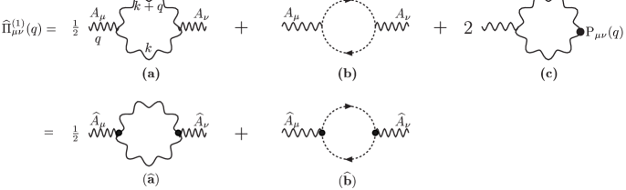
Figure 1: The PT self-energy at one-loop.

Then, the final result is

$$\widehat{\Delta}^{-1}(q^{2})=q^{2}\left[1+bg^{2}\ln\left(\frac{q^{2}}{\mu^{2}}\right)\right]\,,$$ (2.9)

where $b=11C_{A}/48\pi^{2}$ is the first coefficient of the QCD $\beta$-function.

Evidently, due to the Abelian WIs satisfied by the PT effective Green’s functions, the new propagator-like quantity $\widehat{\Delta}^{-1}(q^{2})$ absorbs all the RG-logs, exactly as happens in QED with the photon self-energy. Equivalently, since $Z_{g}$ and ${\widehat{Z}}_{A}$, the renormalization constants of the gauge-coupling and the effective self-energy, respectively, satisfy the QED relation ${Z}_{g}={\widehat{Z}}^{-1/2}_{A}$, the product ${\widehat{d}}(q^{2})=g^{2}\widehat{\Delta}(q^{2})$ forms a RG-invariant ($\mu$-independent) quantity Watson:1996fg ; Binosi:2002vk ; for large momenta $q^{2}$,

$${\widehat{d}}(q^{2})=\frac{\overline{g}^{2}(q^{2})}{q^{2}}\,,$$ (2.10)

where $\overline{g}^{2}(q^{2})$ is the RG-invariant effective charge of QCD,

$$\overline{g}^{2}(q^{2})=\frac{g^{2}}{1+bg^{2}\ln\left(q^{2}/\mu^{2}\right)}=\frac{1}{b\ln\left(q^{2}/\Lambda^{2}\right)}\,.$$ (2.11)

Of central importance for what follows is the connection between the PT and the BFM. The latter is a special gauge-fixing procedure, implemented at the level of the generating functional. In particular, it preserves the symmetry of the action under ordinary gauge transformations with respect to the background (classical) gauge field $\widehat{A}^{a}_{\mu}$, while the quantum gauge fields $A^{a}_{\mu}$ appearing in the loops transform homogeneously under the gauge group, i.e., as ordinary matter fields which happened to be assigned to the adjoint representation Weinberg:kr . As a result of the background gauge symmetry, the $n$-point functions $\langle 0|T\left[\widehat{A}^{a_{1}}_{\mu_{1}}(x_{1})\widehat{A}^{a_{2}}_{\mu_{2}}(x_{2})\dots\widehat{A}^{a_{n}}_{\mu_{n}}(x_{n})\right]|0\rangle$ are gauge-invariant, in the sense that they satisfy naive, QED-like WIs. Notice, however, that they are not gauge-independent, because they depend explicitly on the quantum gauge-fixing parameter $\xi_{Q}$ used to define the tree-level propagators of the quantum gluons and the three- and four-gluon vertices involving one and two background gluons, respectively Abbott:1980hw . The connection between PT and BFM may be stated as follows: The (gauge-independent) PT effective $n$-point functions ($n=2,3,4$) coincide with the (gauge-dependent) BFM $n$-point functions ($n=2,3,4$ background gluons $\widehat{A}^{a}_{\mu}$ entering) provided that the latter are computed at $\xi_{Q}=1$ (e.g. setting $\xi_{Q}=1$ in the Feynman rules of the Appendix). This connection was first established at one-loop level Denner:1994nn , and was recently shown to persist to all orders in perturbation theory Binosi:2002ft .

II.2 The SD equation of the effective gluon self-energy

The structure of the effective gluon self-energy, as it emerges from the all-order PT-BFM correspondence, can be written in a closed non-perturbative form, which coincides with the SD equation for $\widehat{\Delta}$, derived formally from the BFM path integral using functional techniques Sohn:1985em .

In what follows we assume dimensional regularization, and employ the short-hand notation $[dk]=d^{d}k/(2\pi)^{d}$  , where $d=4-\epsilon$ is the dimension of space-time. We refer to diagrams containing one explicit integration over virtual momenta as “one-loop dressed” and those with two integrations as “two-loop dressed”.

We will classify the corresponding diagrams into four categories: one-loop dressed gluonic contribution (group a), one-loop dressed ghost contribution (group b), two-loop dressed gluonic contribution (group c), and two-loop dressed ghost contribution (group d).

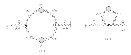
Figure 2: The gluonic contribution at one-loop dressed expansion. Wavy lines with grey blobs represent full-quantum gluon propagators. All external wavy lines (ending with a vertical line) are background gluons. The black dots are the tree-level vertices in the BFM, and the white-blob denote the full three-gluon vertex with one background gluon.

The closed expressions corresponding to the two diagrams of Fig. 2 are given by

$$\widehat{\Pi}^{ab}_{\mu\nu}(q)\big{|}_{{\bf a_{1}}} = \frac{1}{2}\,\int\!\![dk]\,\widetilde{\Gamma}_{\mu\alpha\beta}^{aex}\Delta^{\alpha\rho}_{ee^{\prime}}(k){\widetilde{{\rm I}\Gamma}}_{\nu\rho\sigma}^{be^{\prime}x^{\prime}}\Delta^{\beta\sigma}_{xx^{\prime}}(k+q)\,,$$

$$\widehat{\Pi}^{ab}_{\mu\nu}(q)\big{|}_{{\bf a_{2}}} = \frac{1}{2}\,\int\!\![dk]\,\widetilde{\Gamma}_{\mu\nu\alpha\beta}^{abex}\Delta^{\alpha\beta}_{ex}(k)\,.$$ (2.12)

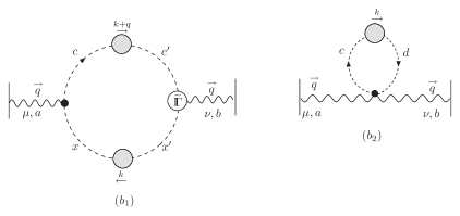
Figure 3: The ghost sector at one-loop dressed expansion. Dashed lines with grey blobs denote full-ghost propagators, while the white blob represents the full background gluon-ghost vertex

For the Fig. 3 we have

$$\widehat{\Pi}^{ab}_{\mu\nu}(q)\big{|}_{{\bf b_{1}}} = -\,\int\!\![dk]\,\widetilde{\Gamma}_{\mu}^{aex}D_{ee^{\prime}}(k){\widetilde{{\rm I}\Gamma}}_{\nu}^{be^{\prime}x^{\prime}}D_{xx^{\prime}}(k+q)\,,$$

$$\widehat{\Pi}^{ab}_{\mu\nu}(q)\big{|}_{{\bf b_{2}}} = -\int\!\![dk]\,\,\widetilde{\Gamma}_{\mu\nu}^{abex}D_{ex}(k)\,.$$ (2.13)

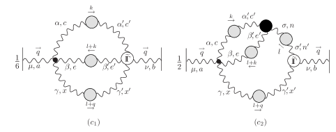
Figure 4: Purely gluonic graphs relevant for the two-loop dressed expansion. The black blob represents the full conventional three-gluon vertex, while the white blobs denote three or four-gluon vertices with one external background leg.

The two-loop dressed gluonic contribution, Fig. 4, reads

$$\widehat{\Pi}^{ab}_{\mu\nu}(q)\big{|}_{{\bf c_{1}}} = \frac{1}{6}\,\int\!\!\int\!\![dk][d\ell]\,\widetilde{\Gamma}_{\mu\alpha\beta\gamma}^{acex}\Delta^{\alpha\alpha^{\prime}}_{cc^{\prime}}(k)\Delta^{\beta\beta^{\prime}}_{ee^{\prime}}(k+\ell)\Delta^{\gamma\gamma^{\prime}}_{xx^{\prime}}(\ell+q){\widetilde{{\rm I}\Gamma}}_{\nu\gamma^{\prime}\beta^{\prime}\alpha^{\prime}}^{bx^{\prime}e^{\prime}c^{\prime}}\,,$$

$$\widehat{\Pi}^{ab}_{\mu\nu}(q)\big{|}_{{\bf c_{2}}} = \frac{1}{2}\,\,\int\!\!\int\!\![dk][d\ell]\,\widetilde{\Gamma}_{\mu\alpha\beta\gamma}^{acex}\Delta^{\alpha\alpha^{\prime}}_{cc^{\prime}}(k)\Delta^{\beta\beta^{\prime}}_{ee^{\prime}}(k+\ell){{\rm I}\Gamma}_{\sigma\beta^{\prime}\alpha^{\prime}}^{ne^{\prime}c^{\prime}}\Delta^{\sigma\sigma^{\prime}}_{nn^{\prime}}(\ell){\widetilde{{\rm I}\Gamma}}_{\nu\gamma^{\prime}\sigma}^{bx^{\prime}n^{\prime}}\Delta^{\gamma\gamma^{\prime}}_{xx^{\prime}}(\ell+q)\,.$$

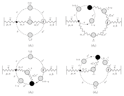
Figure 5: The ghost sector contribution to the two-loop dressed expansion. The black blobs are the conventional full gluon-ghost vertices, while the white ones represent ghost vertices with an (external) background gluon and two ghosts.

The last group represents the two-loop dressed ghost contribution, Fig. 5, and is written as

$$\widehat{\Pi}^{ab}_{\mu\nu}(q)\big{|}_{{\bf d_{1}}} = -\int\!\!\int\!\![dk][d\ell]\,\widetilde{\Gamma}_{\mu\alpha}^{acex}D_{cc^{\prime}}(k+\ell)\Delta^{\alpha\alpha^{\prime}}_{ee^{\prime}}(k)D_{xx^{\prime}}(\ell-q){\widetilde{{\rm I}\Gamma}}_{\nu\alpha^{\prime}}^{bx^{\prime}e^{\prime}c^{\prime}}\,,$$

$$\widehat{\Pi}^{ab}_{\mu\nu}(q)\big{|}_{{\bf d_{2}}} = -\,\,\int\!\!\int\!\![dk][d\ell]\,\widetilde{\Gamma}_{\mu\alpha}^{acex}D_{cc^{\prime}}(k+\ell)D_{ee^{\prime}}(\ell-q){{\rm I}\Gamma}_{\beta}^{e^{\prime}nc^{\prime}}\Delta^{\beta\beta^{\prime}}_{nn^{\prime}}(k+q){\widetilde{{\rm I}\Gamma}}_{\nu\alpha^{\prime}\beta^{\prime}}^{bx^{\prime}n^{\prime}}\Delta^{\alpha\alpha^{\prime}}_{xx^{\prime}}(k)\,,$$

$$\widehat{\Pi}^{ab}_{\mu\nu}(q)\big{|}_{{\bf d_{3}}} = -\,\,\int\!\!\int\!\![dk][d\ell]\,\widetilde{\Gamma}_{\mu\alpha}^{acex}D_{xx^{\prime}}(\ell-q)\Delta^{\alpha\alpha^{\prime}}_{ee^{\prime}}(k){{\rm I}\Gamma}_{\alpha^{\prime}}^{x^{\prime}e^{\prime}n}D_{cc^{\prime}}(k+\ell){\widetilde{{\rm I}\Gamma}}_{\nu}^{bn^{\prime}c^{\prime}}D_{nn^{\prime}}(k+\ell-q)\,,$$

$$\widehat{\Pi}^{ab}_{\mu\nu}(q)\big{|}_{{\bf d_{4}}} = -\,\,\int\!\!\int\!\![dk][d\ell]\,\widetilde{\Gamma}_{\mu\alpha}^{acex}D_{cc^{\prime}}(k+\ell)\Delta^{\alpha\alpha^{\prime}}_{ee^{\prime}}(k){{\rm I}\Gamma}_{\alpha^{\prime}}^{ne^{\prime}c^{\prime}}D_{nn^{\prime}}(\ell){\widetilde{{\rm I}\Gamma}}_{\nu}^{bx^{\prime}n^{\prime}}D_{xx^{\prime}}(\ell-q)\,.$$ (2.15)

Notice that, (i) as explained in the Introduction, the propagators appearing inside the loops are quantum ones, and (ii) there are two general types of vertices, those where all incoming fields are quantum, and those where one of the incoming fields is background.

II.3 Special transversality properties

It is well-known that in the conventional formulation, the diagram containing the ghost-loop (graph ${\bf(b)}$ in Fig. 1) is instrumental for the transversality of $\Pi_{\mu\nu}(q)$. On the other hand, in the PT-BFM scheme, due to the special Feynman rules (see Appendix), the contributions of graphs ${\bf(\widehat{a})}$ and ${\bf(\widehat{b})}$ are individually transverse. Specifically, keeping only the logarithmic terms, one has Abbott:1980hw

$$\widehat{\Pi}_{\mu\nu}^{{\bf(\widehat{a})}}(q)=\frac{10\,C_{A}}{48\pi^{2}}g^{2}\ln\left(\frac{q^{2}}{\mu^{2}}\right){\rm P}_{\mu\nu}(q)\,,\,\,\,\,\widehat{\Pi}_{\mu\nu}^{{\bf(\widehat{b})}}(q)=\frac{C_{A}}{48\pi^{2}}g^{2}\ln\left(\frac{q^{2}}{\mu^{2}}\right){\rm P}_{\mu\nu}(q)\,.$$ (2.16)

In this subsection we will show that, by virtue of the all-order WI satisfied by the full vertices appearing in the diagrams defining $\widehat{\Pi}_{\mu\nu}(q)$, Figs.(2-5), the above property is valid non-perturbatively, and that gluonic and ghost contributions are separately transverse. In addition, the one-loop and two-loop dressed diagrams do not mix. This is to be contrasted to what happens to the conventional case, where the orders of the loop expansion also mix.

There are four fully dressed vertices with one incoming background gluon appearing in the diagrammatic definition of $\widehat{\Pi}_{\mu\nu}(q)$, in Figs.(2-5): ${\widetilde{{\rm I}\Gamma}}_{\mu\alpha\beta}^{abc}$, ${\widetilde{{\rm I}\Gamma}}_{\mu}^{acb}$, ${\widetilde{{\rm I}\Gamma}}_{\mu\nu\alpha\beta}^{abcd}$, ${\widetilde{{\rm I}\Gamma}}_{\mu\nu}^{cdba}$. As is known from formal considerations (see Gambino:1999ai , and references therein), the WI obtained when contracting such vertices with the momentum carried by the background gluon retain to all-orders the same form as at tree-level. The tree-level WI for ${\widetilde{{\rm I}\Gamma}}_{\mu\alpha\beta}^{abc}$ and ${\widetilde{{\rm I}\Gamma}}_{\mu}^{acb}$ are simply

$$q^{\mu}\widetilde{\Gamma}_{\mu\alpha\beta}^{abc}(q,p_{1},p_{2})=gf^{abc}(p_{1}^{2}-p_{2}^{2})g_{\alpha\beta}\,,\,\,\,\ q^{\mu}\widetilde{\Gamma}_{\mu}^{acb}(q,p_{1},p_{2})=gf^{abc}(p_{1}^{2}-p_{2}^{2})\,.$$ (2.17)

In addition, the fact that the four-gluon vertex with one incoming background gluon, and the conventional one (four quantum gluons) coincide at tree-level, as shown in Eq.(A-5), furnishes the corresponding tree-level WI for ${\widetilde{{\rm I}\Gamma}}_{\mu\nu\alpha\beta}^{abcd}$ (see, for instance Papavassiliou:1992ia ). Therefore, the only ingredient missing is the tree-level identity satisfied by ${\widetilde{{\rm I}\Gamma}}_{\mu\nu}^{cdba}$; we now proceed to its derivation.

Contracting the bare vertex $\widetilde{\Gamma}_{\mu\nu}^{cdba}=-ig^{2}f^{acx}f^{xdb}g_{\mu\nu}$, shown in Fig. A-9, with the momentum $q_{1}$ carried by the background gluon, we have that

$$q_{1}^{\mu}\widetilde{\Gamma}_{\mu\nu}^{cdba}(q_{1},q_{2},q_{3},q_{4})=-ig^{2}f^{acx}f^{xdb}q_{1\nu}=ig^{2}\left(f^{abx}f^{cdx}+f^{adx}f^{bcx}\right)q_{1\nu}\,,$$ (2.18)

where we have used the Jaccobi identity

$$f^{abx}f^{cdx}+f^{acx}f^{dbx}+f^{adx}f^{bcx}=0\,.$$ (2.19)

Next we use that

$$0=-\left(f^{abx}f^{cdx}+f^{acx}f^{dbx}+f^{adx}f^{bcx}\right)(q_{1}+q_{4})_{\nu}\,,$$ (2.20)

and add it by parts to (2.18), obtaining

$$q_{1}^{\mu}\widetilde{\Gamma}_{\mu\nu}^{cdba} = ig^{2}\left[f^{cdx}f^{axb}q_{4\nu}+f^{cbx}f^{adx}q_{4\nu}+f^{cax}f^{xdb}(q_{1}+q_{4})_{\nu}\right]$$

$$= -ig\left[f^{cdx}\Gamma_{\nu}^{axb}(q_{4},q_{2}+q_{1},q_{3})+f^{cbx}\Gamma_{\nu}^{adx}(q_{4},q_{2},q_{3}+q_{1})+f^{cax}\Gamma_{\nu}^{xdb}(q_{4}+q_{1},q_{2},q_{3})\right]\,.$$

Armed with the above tree-level results, we proceed to state the four fundamental all-order WIs. First, the WI of the three-field vertices, where on the RHS we have differences of inverse propagators, are given by

$$q_{1}^{\mu}{\widetilde{{\rm I}\Gamma}}_{\mu\alpha\beta}^{abc}(q_{1},q_{2},q_{3}) = gf^{abc}\left[\Delta^{-1}_{\alpha\beta}(q_{2})-\Delta^{-1}_{\alpha\beta}(q_{3})\right]\,,$$

$$q_{1}^{\mu}{\widetilde{{\rm I}\Gamma}}_{\mu}^{acb}(q_{2},q_{1},q_{3}) = gf^{abc}\left[D^{-1}(q_{2})-D^{-1}(q_{3})\right]\,.$$ (2.22)

Then, the WI of the four-field vertices, where on the RHS we have sums of three trilinear vertices, with appropriately shifted arguments, are

$$q_{1}^{\mu}{\widetilde{{\rm I}\Gamma}}_{\mu\nu\alpha\beta}^{abcd}(q_{1},q_{2},q_{3},q_{4})= igf^{abx}{{\rm I}\Gamma}_{\alpha\beta\nu}^{cdx}(q_{3},q_{4},q_{1}+q_{2})$$ (2.23)

$$+ igf^{acx}{{\rm I}\Gamma}_{\beta\nu\alpha}^{dbx}(q_{4},q_{2},q_{1}+q_{3})$$

$$+ igf^{adx}{{\rm I}\Gamma}_{\nu\alpha\beta}^{bcx}(q_{2},q_{3},q_{1}+q_{4})\,,$$

and

$$q_{1}^{\mu}{\widetilde{{\rm I}\Gamma}}_{\mu\nu}^{cdba}(q_{1},q_{2},q_{3},q_{4})= -igf^{cdx}{\rm I}\Gamma_{\nu}^{axb}(q_{4},q_{2}+q_{1},q_{3})$$ (2.24)

$$-igf^{cbx}{\rm I}\Gamma_{\nu}^{adx}(q_{4},q_{2},q_{3}+q_{1})$$

$$-igf^{cax}{\rm I}\Gamma_{\nu}^{xdb}(q_{4}+q_{1},q_{2},q_{3})\,.$$

Notice that Eq.(2.24) is the all-order generalization of (LABEL:WI4b).

With the above WI we can prove that the four groups presented before are independently transverse. We start with group (a): we contract graph (${\bf a_{1}}$) using the first all-order WI of (2.22), whereas for (${\bf a_{2}}$) we simply compute the divergence of the tree-level vertex (A-6), arriving at

$$q^{\nu}\widehat{\Pi}^{ab}_{\mu\nu}(q)\big{|}_{{\bf a_{1}}} = C_{A}\,g^{2}\delta^{ab}\,q_{\mu}\,\int\!\![dk]\,\Delta^{\rho}_{\rho}(k)\,,$$

$$q^{\nu}\widehat{\Pi}^{ab}_{\mu\nu}(q)\big{|}_{{\bf a_{2}}} = -C_{A}\,g^{2}\delta^{ab}\,q_{\mu}\,\int\!\![dk]\,\Delta^{\rho}_{\rho}(k)\,,$$ (2.25)

Thus,

$$q^{\nu}\left(\widehat{\Pi}^{ab}_{\mu\nu}(q)\big{|}_{{\bf a_{1}}}+\widehat{\Pi}^{ab}_{\mu\nu}(q)\big{|}_{{\bf a_{2}}}\right)=0\,.$$ (2.26)

Similarly, the one-loop-dressed ghost contributions of group (b) give upon contraction

$$q^{\nu}\widehat{\Pi}^{ab}_{\mu\nu}(q)\big{|}_{{\bf b_{1}}} = 2\,C_{A}\,g^{2}\delta^{ab}\,q_{\nu}\,\int\!\![dk]\,D(k)\,,$$

$$q^{\nu}\widehat{\Pi}^{ab}_{\mu\nu}(q)\big{|}_{{\bf b_{2}}} = -2\,C_{A}\,g^{2}\delta^{ab}\,q_{\nu}\,\int\!\![dk]\,D(k)\,.$$ (2.27)

and so

$$q^{\nu}\left(\widehat{\Pi}^{ab}_{\mu\nu}(q)\big{|}_{{\bf b_{1}}}+\widehat{\Pi}^{ab}_{\mu\nu}(q)\big{|}_{{\bf b_{2}}}\right)=0\,.$$ (2.28)

The two-loop dressed demonstration is slightly more involved, but essentially straightforward. We begin with the two-loop gluonic contributions (group c). The action of $q^{\nu}$ on the all-order four-gluon vertex ${\widetilde{{\rm I}\Gamma}}_{\nu\gamma^{\prime}\beta^{\prime}\alpha^{\prime}}^{bx^{\prime}e^{\prime}c^{\prime}}(-q,\ell+q,-k-\ell,k)$ appearing on the RHS of the first equation in (LABEL:groupc) may be obtained from (2.23), through the following definition of momenta, $q_{1}=-q$, $q_{2}=\ell+q$, $q_{3}=-k-\ell$, $q_{4}=k$, and corresponding relabellings of Lorentz and color indices. Then,

$$q^{\nu}\widehat{\Pi}^{ab}_{\mu\nu}(q)\big{|}_{{\bf c_{1}}} = \frac{1}{6}\,ig\,\int\!\!\int\!\![dk][d\ell]\,\widetilde{\Gamma}_{\mu\alpha\beta\gamma}^{acex}\Delta^{\alpha\alpha^{\prime}}(k)\Delta^{\beta\beta^{\prime}}(k+\ell)\Delta^{\gamma\gamma^{\prime}}(\ell+q)[$$

$$f^{bxi}{{\rm I}\Gamma}_{\beta^{\prime}\alpha^{\prime}\gamma^{\prime}}^{eci}(-k-\ell,k,\ell)+f^{bei}{{\rm I}\Gamma}_{\alpha^{\prime}\gamma^{\prime}\beta^{\prime}}^{cxi}(k,\ell+q,-k-\ell-q)+$$

$$f^{bci}{{\rm I}\Gamma}_{\gamma^{\prime}\beta^{\prime}\alpha^{\prime}}^{xei}(\ell+q,-k-\ell,k-q)]\,.$$

It is not difficult to verify that, after judicious shifting and relabelling of the integration momenta and of the “dummy” Lorentz and color indices, the three terms on the RHS of (II.3) are in fact equal. Thus,

$$q^{\nu}\widehat{\Pi}^{ab}_{\mu\nu}(q)\big{|}_{{\bf c_{1}}}=\frac{1}{2}\,igf^{bxi}\,\int\!\!\int\!\![dk][d\ell]\,\widetilde{\Gamma}_{\mu\alpha\beta\gamma}^{acex}\Delta^{\alpha\alpha^{\prime}}(k)\Delta^{\beta\beta^{\prime}}(k+\ell)\Delta^{\gamma\gamma^{\prime}}(\ell+q){{\rm I}\Gamma}_{\beta^{\prime}\alpha^{\prime}\gamma^{\prime}}^{eci}(-k-\ell,k,\ell)\,.$$ (2.30)

The other graph gives

$$q^{\nu}\widehat{\Pi}^{ab}_{\mu\nu}(q)\big{|}_{{\bf c_{2}}} = \frac{1}{2}\,ig\,f^{bxi}\,\int\!\!\int\!\![dk][d\ell]\,\widetilde{\Gamma}_{\mu\alpha\beta\gamma}^{acex}\Delta^{\alpha\alpha^{\prime}}(k)\Delta^{\beta\beta^{\prime}}(k+\ell){{\rm I}\Gamma}_{\gamma^{\prime}\beta^{\prime}\alpha^{\prime}}^{iec}(\ell,-k-\ell,k)\Delta^{\gamma^{\prime}\gamma}(\ell+q)$$

$$- \frac{1}{2}\,ig\,f^{bxi}\,\int\!\!\int\!\![dk][d\ell]\,\widetilde{\Gamma}_{\mu\alpha\beta\gamma}^{acex}\Delta^{\alpha\alpha^{\prime}}(k)\Delta^{\beta\beta^{\prime}}(k+\ell){{\rm I}\Gamma}_{\gamma^{\prime}\beta^{\prime}\alpha^{\prime}}^{iec}(\ell,-k-\ell,k)\Delta^{\gamma^{\prime}\gamma}(\ell)\,.$$

Evidently the second term on the RHS of (LABEL:c2) vanishes identically, since the integral is independent of $q$, and therefore the free Lorentz index $\mu$ cannot be saturated.

We then observe that, due to the full Bose symmetry of the conventional three-gluon vertex, ${{\rm I}\Gamma}_{\beta^{\prime}\alpha^{\prime}\gamma^{\prime}}^{eci}(-k-\ell,k,\ell)={{\rm I}\Gamma}_{\gamma^{\prime}\beta^{\prime}\alpha^{\prime}}^{iec}(\ell,-k-\ell,k)$, and therefore, finally,

$$q^{\nu}\left(\widehat{\Pi}^{ab}_{\mu\nu}(q)\big{|}_{{\bf c_{1}}}+\widehat{\Pi}^{ab}_{\mu\nu}(q)\big{|}_{{\bf c_{2}}}\right)=0\,.$$ (2.32)

Finally, we turn to the two-loop-dressed ghost-graphs (group d). For the calculation of the divergence of graph (${\bf d_{1}}$) we use Eq.(2.24); this WI generates three distinct terms, i.e.

$$q^{\nu}\widehat{\Pi}^{ab}_{\mu\nu}(q)\big{|}_{{\bf d_{1}}} = -\,ig\,\int\!\!\int\!\![dk][d\ell]\,\widetilde{\Gamma}_{\mu\alpha}^{acex}D(k+\ell)\Delta^{\alpha\beta}(k)\,D(\ell-q)[$$

$$f^{ebi}{{\rm I}\Gamma}_{\beta}^{xic}(q-\ell,-k-q,k+\ell)+f^{bci}{{\rm I}\Gamma}_{\beta}^{xei}(q-\ell,-k,k+\ell-q)$$

$$+ f^{bxi}{{\rm I}\Gamma}_{\beta}^{iec}(-\ell,-k,k+\ell)]\,.\,$$

Each one of these three terms can be easily shown to cancel exactly against the individual divergences of the remaining three graphs. To see this in detail, use the first WI of (2.22) for graph $({\bf d_{2}})$, and the second of (2.22) for graphs $({\bf d_{3}})$ and $({\bf d_{4}})$. In all three cases one of the two inverse propagators generated by the WI will give rise to an expression similar to the second term on the RHS of (LABEL:c2), i.e. a $q$-independent integral with a free Lorentz index, which cannot be saturated. These three terms are directly set to zero. The terms stemming from the other inverse propagator read:

$$q^{\nu}\widehat{\Pi}^{ab}_{\mu\nu}(q)\big{|}_{{\bf d_{2}}} = \,igf^{bei}\,\int\!\!\int\!\![dk][d\ell]\,\widetilde{\Gamma}_{\mu\alpha}^{acex}\,D(k+\ell)\Delta^{\alpha\beta}(k)\,D(\ell-q){{\rm I}\Gamma}_{\beta}^{cxi}(k+\ell,q-\ell,-k-q)\,,$$

$$q^{\nu}\widehat{\Pi}^{ab}_{\mu\nu}(q)\big{|}_{{\bf d_{3}}} = \,igf^{bci}\,\int\!\!\int\!\![dk][d\ell]\,\widetilde{\Gamma}_{\mu\alpha}^{acex}\,D(k+\ell)\Delta^{\alpha\beta}(k)\,D(\ell-q){{\rm I}\Gamma}_{\beta}^{ixe}(\ell+k-q,q-\ell,-k)\,,$$

$$q^{\nu}\widehat{\Pi}^{ab}_{\mu\nu}(q)\big{|}_{{\bf d_{4}}} = \,igf^{bxi}\,\int\!\!\int\!\![dk][d\ell]\,\widetilde{\Gamma}_{\mu\alpha}^{acex}\,D(k+\ell)\Delta^{\alpha\beta}(k)\,D(\ell-q){{\rm I}\Gamma}_{\beta}^{cie}(k+\ell,-\ell,-k)\,.$$

and, as announced, can be directly identified with the corresponding terms on the RHS of (II.3). Therefore,

$$q^{\nu}\left(\widehat{\Pi}^{ab}_{\mu\nu}(q)\big{|}_{{\bf d_{1}}}+\widehat{\Pi}^{ab}_{\mu\nu}(q)\big{|}_{{\bf d_{2}}}+\widehat{\Pi}^{ab}_{\mu\nu}(q)\big{|}_{{\bf d_{3}}}+\widehat{\Pi}^{ab}_{\mu\nu}(q)\big{|}_{{\bf d_{4}}}\right)=0\,.$$ (2.35)

This concludes the non-perturbative proof of the special transversality property of $\widehat{\Pi}^{ab}_{\mu\nu}(q)$: gluon and ghost loops are separately transverse, and the loops of different order do not mix

II.4 Towards a new SD series

As explained for the first time in Cornwall:1982zr , the upshot the PT is to eventually trade the conventional SD series for another, written in terms of the new, gauge-independent building blocks. Then one could truncate this new series, by keeping only a few terms in a “dressed-loop” expansion, and maintain exact gauge-invariance, while at the same time accommodating non-perturbative effects. As mentioned in the Introduction, one of the most central issues in this context is how to convert the SD-series defining $\widehat{\Delta}_{\mu\nu}$ into a dynamical equation, namely one that contains $\widehat{\Delta}_{\mu\nu}$ on both sides. For this to become possible, one must carry out inside the loops of the diagrams shown in the previous subsection the substitution ${\Delta}_{\mu\nu}\to\widehat{\Delta}_{\mu\nu}$. In this subsection we focus only on one particular aspect of this problem, namely the role that the BQIs might play in implementing the aforementioned substitution.

The connection Binosi:2002ez between the PT and the Batalin-Vilkovisky quantization formalism Batalin:pb has been instrumental for various of the recent developments in the PT. Specifically, using the formulation of the BFM within this latter formalism, one can derive non-trivial identities (BQI’s), relating the BFM $n$-point functions to the corresponding conventional $n$-point functions in the covariant renormalizable gauges, to all orders in perturbation theory Gambino:1999ai . The relation between these two types of $n$-point functions is written in a closed form by means of a set of auxiliary Green’s functions involving anti-fields and background sources, introduced in the BFM formulation. These latter Green’s functions are in turn related by means of a SD type of equation  Binosi:2002ez to the conventional ghost Green’s functions appearing in the STI satisfied by the conventional all-order three-gluon vertex Bar-Gadda:1979cz ; Ball:1980ax ; PasTar .

We will restrict our discussion to the case of the propagators $\widehat{\Delta}_{\mu\nu}$ and ${\Delta}_{\mu\nu}$. The relevant quantity appearing in the corresponding BQI is the following two-point function, to be denoted by $\Lambda_{\alpha\beta}(q)$, defined as (we suppress color indices)

$$\Lambda_{\alpha\beta}(q)=\int\![dk]H^{(0)}_{\alpha\mu}D(k)\Delta^{\mu\nu}(k+q)\,H_{\beta\nu}^{*}(k+q,-k,-q),$$ (2.36)

where the elementary vertex $H_{\alpha\beta}^{(0)}$ is

and $H_{\alpha\beta}$ is given by

(2.37)

with $q+p+r=0$. ${\cal K}_{\nu\beta}$ is the conventional one-particle irreducible connected ghost-ghost-gluon-gluon kernel appearing in the QCD skeleton expansion Marciano:su ; Bar-Gadda:1979cz . Notice that $H_{\alpha\beta}$ appears in the all-order Slavnov-Taylor identity satisfied by the conventional three-gluon vertex Ball:1980ax , and is related to the conventional gluon-ghost vertex ${{\rm I}\Gamma}_{\beta}(p,r,q)$ by Marciano:su ; Bar-Gadda:1979cz ; PasTar ,

$$q^{\alpha}H_{\alpha\beta}(p,r,q)={{\rm I}\Gamma}_{\beta}(p,r,q)\,.$$ (2.38)

Using the diagrammatic definition of $H_{\alpha\beta}$ shown in Eq.(2.37), we may recast Eq.(2.36) in a dressed-loop expansion as follows,

(2.39)

Due to the transversality of both $\widehat{\Pi}_{\mu\nu}(q)$ and $\Pi_{\mu\nu}(q)$, if we write

$$\Lambda_{\alpha\beta}(q)=g_{\alpha\beta}G(q^{2})+q_{\alpha}q_{\beta}L(q^{2}),$$ (2.40)

it turns out that the fundamental all-order BQI between $\Delta(q)$ and $\widehat{\Delta}(q)$ involves only $G(q^{2})$, and is given by Gambino:1999ai ; Binosi:2002ez

$$\widehat{\Delta}(q)=\left[1+G(q)\right]^{2}\,\Delta(q)\,.$$ (2.41)

It is then elementary to demonstrate that the full propagators (in the Feynman gauge) are related by

$$\Delta_{\mu\nu}(q)=\left[1+G(q)\right]^{2}\widehat{\Delta}_{\mu\nu}(q)-iG(q^{2})\,\left[1+G(q)\right]\,\frac{q_{\mu}q_{\nu}}{q^{4}}\,.$$ (2.42)

The process of replacing $\Delta_{\mu\nu}\to\widehat{\Delta}_{\mu\nu}$ will therefore introduce the function $G$ inside the loops; however, the theoretical and practical consequences of this operation are not clear to us at this point. Some of the various possibilities that one might envisage include: to study the dynamical equation for $G$ (viz. Eq. (2.36)) together with the SD of $\widehat{\Delta}$, as a coupled system Grassi:2004yq ; attempt to reabsorb the $G$’s into a redefinition of the vertices appearing in the diagrams, together with their corresponding SD equations; consider the diagrams containing $G^{\prime}s$ as being of higher order in the dressed loop expansion, due to the additional explicit integration appearing in their definition, Eq. (2.36).

In the rest of this article we will adopt what appears to be the lowest order approximation in this context, setting $\Delta_{\mu\nu}=\widehat{\Delta}_{\mu\nu}$ in the SD equation, and $G=0$ everywhere else.

III General considerations for IR finite solutions

In this section we will briefly review some of the main issues involved when trying to obtain from the corresponding SD equation IR finite solutions for the gluon self-energy $\widehat{\Delta}$. By “IR finite” we mean solutions for which $\widehat{\Delta}^{-1}(0)\neq 0$, which is equivalent to saying that $\widehat{\Delta}(0)$ is finite.

III.1 Two necessary conditions

Let us start by considering two necessary conditions for obtaining IR finite solutions.

(i) From the one-loop dressed SD equation for the gluon self-energy (see Fig. 2) it is clear that, since there can be at most two full gluon self-energies inside the diagrams, on dimensional grounds the value of $\widehat{\Delta}^{-1}(0)$ will in general be proportional to two types of seagull-like contributions,

$${\cal T}_{0} = \int\!\,[dk]\,\widehat{\Delta}(k)\,,$$

$${\cal T}_{1} = \int\!\,[dk]\,k^{2}\,\widehat{\Delta}^{2}(k)\,.$$ (3.1)

Perturbatively, both ${\cal T}_{0}$ and ${\cal T}_{1}$ vanish by virtue of the dimensional regularization result

$$\int\!\!\frac{[dk]}{k^{2}}\ln^{N}(k^{2})=0\,,\quad N=0,1,2,\ldots$$ (3.2)

which guarantees the masslessness of the gluon to all orders in perturbation theory. In order to permit IR finite solutions one must assume that seagull-like contributions, such as those shown in (3.1), do not vanish non-perturbatively. Of course, once assumed non-vanishing, both ${\cal T}_{0}$ and ${\cal T}_{1}$ are quadratically divergent, and, in order to make sense out of them, a suitable regularization must be employed.

(ii) The form of the full three-gluon vertex is instrumental for the generation of IR finite solutions. Specifically, as is well known from the classic papers on dynamical mass generation Jackiw:1973tr , in order to obtain $\widehat{\Delta}^{-1}(0)\neq 0$ one must introduce massless poles in the full three-gluon vertex ${\widetilde{{\rm I}\Gamma}}_{\nu\alpha\beta}$, appearing in the expression for $\widehat{\Pi}_{\mu\nu}^{(\bf{a_{1}})}(q)$, Eq.(2.12)  Baker:1980gf . Notice in particular that, whereas after allowing for non-vanishing seagull contributions the inclusion of graph $(\bf{a_{2}})$ is essential for the transversality of $\widehat{\Pi}_{\mu\nu}$, its presence does not lead to $\widehat{\Delta}^{-1}(0)\neq 0$. Thus, if the full three-gluon vertex $\widetilde{{\rm I}\Gamma}$ satisfies the WI of (2.22), but does not contain poles, then the seagull contribution ${\cal T}_{0}\neq 0$ of graph $({\bf a_{2}})$ will cancel exactly against analogous contributions contained in graph $({\bf a_{1}})$, forcing $\widehat{\Delta}^{-1}(0)=0$. Put in a different way, the non-vanishing seagull contribution that will determine the value of $\widehat{\Delta}^{-1}(0)$ is not the one coming from graph $({\bf a_{2}})$. This is even more evident in the non-linear treatment, where the term ${\cal T}_{1}$ makes its appearance; clearly, such a term cannot be possibly obtained from $({\bf a_{2}})$.

To appreciate the delicate interplay between the points mentioned above, let us consider the ghostless, one-loop dressed version of the SD equation, by keeping only the two graphs of group (a). The SD equation has the general form,

$$\widehat{\Delta}^{-1}(q^{2}){\rm P}_{\mu\nu}(q)=q^{2}{\rm P}_{\mu\nu}(q)+i\left[\widehat{\Pi}_{\mu\nu}^{(\bf{a_{1}})}(q)+\widehat{\Pi}_{\mu\nu}^{(\bf{a_{2}})}\right]\,,$$ (3.3)

with

$$\widehat{\Pi}_{\mu\nu}^{(\bf{a_{1}})}(q) = \frac{1}{2}\,C_{A}\,g^{2}\,\int\!\![dk]\widetilde{\Gamma}_{\mu\alpha\beta}\widehat{\Delta}^{\alpha\alpha^{\prime}}(k){\widetilde{{\rm I}\Gamma}}_{\nu\alpha^{\prime}\beta^{\prime}}\widehat{\Delta}^{\beta\beta^{\prime}}(k+q)\,,$$

$$\widehat{\Pi}_{\mu\nu}^{(\bf{a_{2}})} = -C_{A}\,g^{2}\,g_{\mu\nu}{\cal T}_{0}\,.$$ (3.4)

Let us write $i\widehat{\Pi}_{\mu\nu}^{(\bf{a_{1}})}(q)$ in the general form

$$i\widehat{\Pi}_{\mu\nu}^{(\bf{a_{1}})}(q)=q^{2}A(q^{2})g_{\mu\nu}+B(q^{2})q_{\mu}q_{\nu}\,,$$ (3.5)

where $A(q^{2})$ and $B(q^{2})$ are arbitrary dimensionless functions, whose precise expressions depend on the details of the ${\widetilde{{\rm I}\Gamma}}_{\nu\alpha^{\prime}\beta^{\prime}}$ employed.

The transversality of $i\left[\widehat{\Pi}_{\mu\nu}^{(\bf{a_{1}})}(q)+\widehat{\Pi}_{\mu\nu}^{(\bf{a_{2}})}\right]$ implies immediately the condition

$$q^{2}\left[A(q^{2})+B(q^{2})\right]=iC_{A}\,g^{2}\,{\cal T}_{0}\,,$$ (3.6)

and thus the sum of the two graphs reads

$$i\left[\widehat{\Pi}_{\mu\nu}^{(\bf{a_{1}})}(q)+\widehat{\Pi}_{\mu\nu}^{(\bf{a_{2}})}\right]=-q^{2}B(q^{2})P_{\mu\nu}(q)\,.$$ (3.7)

Clearly,

$$\widehat{\Delta}^{-1}(0)={\displaystyle\lim_{q^{2}\to 0}}(-q^{2}B(q^{2}))\,={\displaystyle\lim_{q^{2}\to 0}}(q^{2}A(q^{2}))-iC_{A}\,g^{2}\,{\cal T}_{0}\,.$$ (3.8)

Interestingly enough, once the transversality of $\widehat{\Pi}_{\mu\nu}$ has been enforced, the behavior of $\widehat{\Delta}^{-1}(q^{2})$ is determined solely by $B(q^{2})$. In particular, the value of $\widehat{\Delta}^{-1}(0)$ is given by ${\displaystyle\lim_{q^{2}\to 0}}\left(-q^{2}B(q^{2})\right)$. Evidently, if $B(q^{2})$ does not contain $(1/q^{2})$ terms, one has that ${\displaystyle\lim_{q^{2}\to 0}}(-q^{2}B(q^{2}))=0$, and therefore $\widehat{\Delta}^{-1}(0)=0$, despite the fact that ${\cal T}_{0}$ has been assumed to be non-vanishing. Actually, as we will see in the context of the linearized SD equation that we will study in the next section, if ${\widetilde{{\rm I}\Gamma}}_{\nu\alpha\beta}$ does not contain massless poles, it is precisely this latter situation that is realized, by virtue of an identity relating the various integrals involved. On the other hand, if $B(q^{2})$ contains $(1/q^{2})$ terms, ${\displaystyle\lim_{q^{2}\to 0}}(-q^{2}B(q^{2}))\neq 0$, allowing for $\widehat{\Delta}^{-1}(0)\neq 0$. In fact, for physically acceptable solutions, one must demand that $\widehat{\Delta}^{-1}(0)>0$, which imposes further restrictions on the possible forms of $\widetilde{{\rm I}\Gamma}$. Of course, this is not to say that the presence of poles in the vertex is sufficient for obtaining IR-finite solutions, because $B(q^{2})$ may end up being non-singular due to accidental algebraic cancellations. As we will see in a concrete example in the next section, the net contributions of pole terms originating from different Lorentz structures within the same vertex may lead to an equation that does not generate mass.

The quantities $A(q^{2})$ and $B(q^{2})$ appearing in (3.5), will be functionals of the unknown quantity $\widehat{\Delta}$, as dictated by the SD equation; their specific form will depend on the details of the vertex Ansatz chosen. In general, their value at $q^{2}=0$ will be linear combinations of the two terms defined in (3.1), namely

$$\widehat{\Delta}^{-1}(0)=g^{2}\left(a_{0}{\cal T}_{0}+a_{1}{\cal T}_{1}\right)\,,$$ (3.9)

where the values of the numerical coefficients $a_{0}$ and $a_{1}$ depend on the details of the problem.

Then, the corresponding SD equation will read schematically

$$\widehat{\Delta}^{-1}(q^{2})=\widehat{\Delta}^{-1}(0)+g^{2}q^{2}\int\![dk]\,\,{\cal F}\{\widehat{\Delta};q,k\}\,,$$ (3.10)

where the functional ${\cal F}\{\widehat{\Delta};q,k\}$ is regular at $q^{2}=0$. Then, after renormalizing, we will be looking for solutions of (3.10) that simultaneously: (a) reproduce correctly the asymptotic behavior for $\widehat{\Delta}(q^{2})$ predicted by the RG, viz. Eqs. (2.9) and (2.11); (b) are finite at $q^{2}=0$; (c) satisfy the (appropriately regulated) constraint of (3.9) foot1 . Turns out that points (a), (b), and (c) are deeply intertwined, in a way that we will sketch below, and further elaborate upon in Sec. IV.

III.2 RG behavior and the SD equation

The asymptotic behavior that $\widehat{\Delta}(q^{2})$ must satisfy in the deep UV is given by Eqs. (2.9) and (2.11). In practice, however, it is highly non-trivial to obtain, from the corresponding SD equation, solutions displaying this asymptotic behavior. This difficulty is intimately connected to the approximations used for the (all-order) vertex $\widetilde{{\rm I}\Gamma}$. Of course, within a full SD equation treatment, $\widetilde{{\rm I}\Gamma}$ satisfies its own non-linear integral equation, which determines its structure. One must deal then with a very complex system of coupled integral equations involving $\widehat{\Delta}$, $\widetilde{{\rm I}\Gamma}$, and several many-particle kernels. The usual way to reduce the difficulty of this problem is to resort to the gauge-technique, namely express $\widetilde{{\rm I}\Gamma}$ as a functional of $\widehat{\Delta}$, in such a way as to satisfy (by construction) the first WI of Eq. (2.22) exactly. This procedure fixes the “longitudinal” part of the vertex, but leaves its “transverse” (identically conserved) part undetermined. This ambiguity, in turn, leads to the mishandling of overlapping divergences, which manifests itself in the fact that (i) one cannot renormalize multiplicatively, but only subtractively, and (ii) the RG-behavior of the solutions is distorted. In particular, one obtains solutions which asymptotically behave like

$$\widehat{\Delta}^{-1}(q^{2})=q^{2}\left[1+wbg^{2}\ln\left(\frac{q^{2}}{\mu^{2}}\right)\right]^{1/w}\,,$$ (3.11)

with $w>1$. These solutions reproduce upon expansion the expected (one-loop) perturbative result, but non-perturbatively they miss the correct RG behavior of (2.9).

The first-principle remedy of the situation would require the full treatment of the conserved part of the vertex, in a way similar to that followed in King:1982mk for the vertex appearing in the electron and quark gap equations. Unfortunately, extending their method to the case of the three-gluon vertex is technically very involved, and is at the moment beyond our powers. Instead, we propose to model the RG behavior according to the simple prescription put forth in Cornwall:1982zr ; Cornwall:1985bg . The basic observation is that the correct RGI may be restored if every $\widehat{\Delta}(z)$ appearing inside ${\cal F}\{\widehat{\Delta};q,k\}$ were to be multiplied (“by hand”) by a factor (see Eq.(2.11))

$$1+bg^{2}\ln(z/\mu^{2})=\frac{g^{2}}{\overline{g}^{2}(z)}\,.$$ (3.12)

Thus, one is effectively switching from (3.10) to the corresponding“RG-improved” equation

$$\widehat{\Delta}^{-1}(q^{2})=\widehat{\Delta}^{-1}(0)+g^{2}q^{2}\int\![dk]\,\,{\cal F}\{\widehat{\Delta}(z)\left(g^{2}/\overline{g}^{2}(z)\right);q,k\}\,,$$ (3.13)

with $z=k^{2}$ or $z=(k+q)^{2}$; equivalently, in terms of the manifestly RG-invariant quantities ${\widehat{d}}(q^{2})$ and $\bar{g}^{2}(q^{2})$,

$${\widehat{d}}^{\,-1}(q^{2})={\widehat{d}}^{\,-1}(0)+q^{2}\int\![dk]\,\,{\cal F}\{{\widehat{d}}(z)/\overline{g}^{2}(z);q,k\}$$ (3.14)

and

$${\widehat{d}}^{\,-1}(0)=a_{0}\overline{{\cal T}}_{0}+a_{1}\overline{{\cal T}}_{1}\,,$$ (3.15)

where (in Euclidean space), by virtue of (2.10)

$$\overline{{\cal T}}_{0} = \int\!\,[dk]\frac{{\widehat{d}}(k^{2})}{\overline{g}^{2}(k^{2})}\,,$$

$$\overline{{\cal T}}_{1} = \int\!\,[dk]\,\frac{k^{2}\,{\widehat{d}}^{\,2}(k^{2})}{\overline{g}^{4}(k^{2})}\,.$$ (3.16)

III.3 Regularization of seagull-like terms

Returning the issue of the regulation of the constraint (3.15), notice that the integrals in (3.1) differ from those of (3.16) in an important way. Roughly speaking, the presence of the RG logarithms in their numerators, (contained in $\overline{g}^{2}(k^{2})$ and $\overline{g}^{4}(k^{2})$, respectively) compensates the logarithms contained in ${\widehat{d}}(k^{2})$ and ${\widehat{d}}^{2}(k^{2})$, allowing one to regularize them simply by subtracting a unique (vanishing) integral, that of Eq.(3.2) for $N=0$, provided the solutions satisfy certain generic conditions.

To study this in detail, let us for the moment concentrate on (potential) solutions of the SD equation that are qualitatively of the general form

$${\widehat{d}}(q^{2})=\frac{{\overline{g}}^{2}_{{{\scriptscriptstyle\rm NP}}}(q^{2})}{q^{2}+m^{2}(q^{2})}\,,$$ (3.17)

where

$${\overline{g}}^{2}_{{{\scriptscriptstyle\rm NP}}}(q^{2})=\bigg{[}b\ln\left(\frac{q^{2}+f(q^{2},m^{2}(q^{2}))}{\Lambda^{2}}\right)\bigg{]}^{-1}\,.$$ (3.18)

The function $m^{2}(q^{2})$ may be interpreted as a momentum dependent “mass” with the property (to be imposed self-consistently) that $m^{2}(0)>0$. In addition, we expect that $m^{2}(q^{2})$ is a monotonically decreasing function of $q^{2}$, with $m^{2}(q^{2})\rightarrow 0$ as $q^{2}/\Lambda^{2}\to\infty$. The quantity ${\overline{g}}^{2}_{{{\scriptscriptstyle\rm NP}}}(q^{2})$ represents a non-perturbative version of the RG-invariant effective charge of QCD, going over to $\overline{g}^{2}(q^{2})$ in the deep UV. The (dimensionfull) function $f(q^{2},m^{2}(q^{2}))$ is expected to be such that ${\overline{g}}^{2}_{{{\scriptscriptstyle\rm NP}}}(q^{2})$ will be a monotonically decreasing function of $q^{2}$, with $f(0,m^{2}(0))>\Lambda^{2}$. The dimensionality of $f$ is to be saturated by $m^{2}(q^{2})$; thus if one were to set $m^{2}(q^{2})=0$ then one should have $f(q^{2},0)=0$. The presence of a $f(q^{2},m^{2}(q^{2}))$ with such properties in the logarithm of ${\overline{g}}^{2}_{{{\scriptscriptstyle\rm NP}}}(q^{2})$ eliminates the Landau pole, and leads in the deep IR to the characteristic property of “freezing”. For the analysis that follows, note also that

$$\frac{1}{{\overline{g}}^{2}_{{{\scriptscriptstyle\rm NP}}}(q^{2})}-\frac{1}{\overline{g}^{2}(q^{2})}=b\ln\left(1+\frac{f(q^{2},m^{2}(q^{2}))}{q^{2}}\right)\,.$$ (3.19)

It turns out that, for the proposed regularization to work, both $m^{2}(k^{2})$ and $f(q^{2},m^{2}(q^{2}))$ must drop “sufficiently fast” in the deep UV.

To understand this point, we substitute into $\overline{{\cal T}}_{0}$ of Eq.(3.16) a solution of the form (3.17),

$$\overline{{\cal T}}_{0}=\int\![dk]\frac{{\overline{g}}^{2}_{{{\scriptscriptstyle\rm NP}}}(k^{2})}{[k^{2}+m^{2}(k^{2})]\overline{g}^{2}(k^{2})}\,,$$ (3.20)

and consider $\overline{{\cal T}}_{0}^{\,{{\rm reg}}}$, obtained after subtracting $\int\!\,[dk]/k^{2}=0$ from $\overline{{\cal T}}_{0}$,

$$\overline{{\cal T}}_{0}^{\,{{\rm reg}}} \equiv \int\![dk]\bigg{(}\,\frac{{\overline{g}}^{2}_{{{\scriptscriptstyle\rm NP}}}(k^{2})}{[k^{2}+m^{2}(k^{2})]\overline{g}^{2}(k^{2})}-\frac{1}{k^{2}}\bigg{)}$$ (3.21)

$$= -\int\![dk]\frac{m^{2}(k^{2})}{k^{2}\,[k^{2}+m^{2}(k^{2})]}\,-b\int\![dk]\,{\widehat{d}}(k^{2})\,\ln\left(1+\frac{f(k^{2},m^{2}(k^{2}))}{k^{2}}\right)\,.$$

Let us examine the two integrals on the RHS separately. If $m^{2}(k^{2})$ behaved asymptotically as $\ln^{-a}(k^{2})$, with the anomalous mass-dimension $a>1$, then the first integral would converge, by virtue of the elementary result

$$\int\frac{dz}{z\,(\ln z)^{1+\gamma}}=-\frac{1}{\gamma\,(\ln z)^{\gamma}}\,.$$ (3.22)

Whether such a behavior of $m^{2}(k^{2})$ is realized or not must be verified directly from the corresponding SD equation. For example, this was indeed the case for the equations studied in Cornwall:1982zr ; Cornwall:1985bg , (with $a=12/11$), and we will observe it again in the next section. In fact, a faster asymptotic behavior of the form $\ln^{a}(k^{2})/k^{2}$ may be obtained from non-linear versions of the SD equation Cornwall:1985bg . The second integral will converge as well, provided that $f(k^{2},m^{2}(k^{2}))$ drops asymptotically at least as fast as $\ln^{-c}(k^{2})$, with $c>0$. If, for example, $f=\rho m^{2}(k^{2})$ (with $a>1$, for the first integral to converge), then the convergence condition for the second integral is automatically fulfilled. Notice that perturbatively $\overline{{\cal T}}_{0}^{\,{{\rm reg}}}$ vanishes; this is because $m^{2}(k^{2})=0$ to all orders, and therefore, since in that case also $f=0$, both integrals on the RHS of (3.21) vanish.

Assuming that $m^{2}(k^{2})$ and $f(k^{2},m^{2}(k^{2}))$ behave as described above, then it is straightforward to verify that the difference $\overline{{\cal T}}_{1}-\overline{{\cal T}}_{0}$ is automatically finite. Indeed, applying the elementary identity $k^{2}=[k^{2}+m^{2}(k^{2})]-m^{2}(k^{2})$ in the numerator of $\overline{{\cal T}}_{1}$, we arrive at

$$\overline{{\cal T}}_{1}-\overline{{\cal T}}_{0}=-\int\!\,[dk]\,\frac{m^{2}(k^{2})\,{\widehat{d}}^{\,2}(k^{2})}{\overline{g}^{4}(k^{2})}\,-b\int\![dk]\,\frac{{\overline{g}}^{2}_{{{\scriptscriptstyle\rm NP}}}(k^{2})}{\overline{g}^{2}(k^{2})}{\widehat{d}}(k^{2})\ln\left(1+\frac{f(k^{2},m^{2}(k^{2}))}{k^{2}}\right)\,,$$ (3.23)

where both integrals on the RHS converge, without any additional assumptions.

Thus, the RHS of (3.15) can be written as

$${\widehat{d}}^{\,-1}(0)=(a_{0}+a_{1})\overline{{\cal T}}_{0}+a_{1}(\overline{{\cal T}}_{1}-\overline{{\cal T}}_{0})\,.$$ (3.24)

Clearly, if we happened to have that $a_{1}=-a_{0}$, the RHS of (3.24) would be automatically convergent, without further need of regularization. If $a_{1}\neq-a_{0}$, we will replace on the RHS of (3.24) $\overline{{\cal T}}_{0})$ by $\overline{{\cal T}}_{0}^{\,reg}$, arriving at the regularized version of (3.15)

$${\widehat{d}}^{\,-1}_{{{\rm reg}}}(0)=(a_{0}+a_{1})\overline{{\cal T}}_{0}^{\,{{\rm reg}}}+a_{1}(\overline{{\cal T}}_{1}-\overline{{\cal T}}_{0})\,.$$ (3.25)

It is important to emphasize that the form of the solutions assumed in (3.17) is meant to quantify the UV behavior necessary for the proposed regularization to work, but does not restrict their deep IR behavior. Specifically, let us assume that a solution of the type (3.17), to be denoted by ${\widehat{d}}_{\rm\,C}(q^{2})$, satisfies the necessary asymptotic conditions, and consider a new function, ${\widehat{d}}_{\rm\,N}(q^{2})={\widehat{d}}_{\rm\,C}(q^{2})+h(q^{2})$, where $h(q^{2})$ vanishes faster than ${\widehat{d}}_{\rm\,C}(q^{2})$ in the UV, but is not restricted in the IR. Then, if ${\widehat{d}}_{\rm\,N}(q^{2})$ is inserted into (3.21), the corresponding integrals are still finite. As we will see in Sec. V, this situation does in fact occur: when solving the corresponding SD equation, in addition to the “canonical” solution of the type (3.17), we find solutions that in the UV go over to (3.17), but in the deep IR display a much sharper increase. The point is that these new solutions can be regulated following the same procedure outlined here.

Several comments are now in order.

(i) The above method for regulating the seagull-like terms relies solely on the integration rules of the only known gauge-invariant regularization scheme, namely dimensional regularization, together with the requirement of an appropriate momentum dependence for the dynamical mass. In that sense it is conceptually rather economical, evoking a minimum amount of additional theoretical input.

(ii) The implementation of the proposed regularization hinges crucially on the requirement that, within the given truncation scheme, the RGI behavior can be encoded faithfully into the SD equation, and the logarithmic terms are correctly accounted for. In particular, the compensation (in the UV) of the RG logarithm contained in ${\widehat{d}}(k^{2})$ by the logarithm of $\overline{g}^{-2}(k^{2})$, is essential for the consistency of the ensuing regularization of (3.16). In the absence of the compensating logarithm one would have to subtract instead a term $1/k^{2}\ln k^{2}$ in order to achieve UV convergence. The rules of dimensional regularization allow such a possibility; by virtue of the more general result Collins

$$\int\!\^{\alpha}=0\,,$$ (3.26)

valid for any value of $\alpha$, together with the elementary identity Cornwall:1977sh

$$\bigg{[}1+bg^{2}\ln(k^{2}/\mu^{2})\bigg{]}^{-R}=\frac{1}{\Gamma(R)}\int_{0}^{\infty}dt\,e^{-t}\,t^{R-1}\,(k^{2}/\mu^{2})^{-t\,b\,g^{2}}$$ (3.27)

(valid for $R>0$), one may set

$$\int\frac{[dk]}{k^{2}[1+bg^{2}\ln(k^{2}/\mu^{2})]}=\int_{0}^{\infty}dt\,e^{-t}\,(\mu^{2})^{tbg^{2}}\int\!\![dk]\,(k^{2})^{-(1+tbg^{2})}=0.$$ (3.28)

Subracting such a term would eventually regulate the initial integral in the UV. The problem, however, is in the IR: the logarithm in the denominator of the regulated integral would give rise to the very pathology one has set out to cure in the first place, namely the Landau pole.

(iii) Of course, ${\widehat{d}}^{\,-1}(0)$ must be positive definite (in Euclidean space). The regularization possibility offered by (3.21) was in fact appreciated in Cornwall:1982zr , but was not pursued further, on the grounds of furnishing the “wrong” sign for ${\widehat{d}}^{\,-1}(0)$. In the context of that work this was indeed so, because the three-gluon vertex used (the analogue of $\widetilde{{\rm I}\Gamma}$) was completely fixed, being the tree-level vertex derived from the Lagrangian of the massive gauge invariant Yang-Mills model. After connecting ${\cal T}_{0}$ to the finite vacuum expectation value of a composite scalar field creating $0^{+}$ glueball states, the replacement

$$\int\![dk]\,\Delta(k^{2})\longrightarrow\Delta^{-1}(0)\int\![dk]\,\Delta^{2}(k^{2})$$ (3.29)

was used instead. Assuming that the correct RG-behavior is captured by the corresponding SD equation, then the integral on the RHS of (3.29) converges due to the extra logarithms in the denominator.

In the case we consider here, the sign situation is more involved. The two integrals on the RHS of Eqs. (3.21) are positive definite (assuming that $m^{2}(k^{2})>0$ and $f(k^{2},m^{2}(k^{2}))>0$ in the full range of momenta); thus, the sign of $\overline{{\cal T}}_{0}^{\,{{\rm reg}}}$ is fixed. On the other hand, the sign of the RHS of (3.23) is not definite, since the $\ln z$ appearing in the numerator of the second integral (contained in $\overline{g}^{-2}(k^{2})$) becomes negative at $z<1$. In addition, and perhaps more importantly, the signs of $a_{0}$ and $a_{1}$ are not a-priori known either. This is so because the expression for ${\widehat{d}}^{\,-1}(0)$ is determined not by the (fixed and known) sign of the seagull graph, but from a delicate combination of the coefficients of the pole terms contained in the full three-gluon vertex $\widetilde{{\rm I}\Gamma}$. In our opinion the issue of the sign should be settled within the strict confines of QCD and dimensional regularization. Thus, if a QCD-derived (approximate, to be sure) form for $\widetilde{{\rm I}\Gamma}$ were to yield (after applying the proposed regularization) a negative sign for ${\widehat{d}}^{\,-1}(0)$, then one should be inclined to conclude that the dynamical mass generation is not realized, at least not in the context of the specific truncation scheme.

IV The linearized SD equation

In this section we will study in detail a linearized version of the SD equation obtained in the one-loop dressed approximation, omitting the ghosts. The resulting equation is a close variant of the one presented in Cornwall:1982zr , but displays several distinct features, allowing us to address further points of interest.

IV.1 Linearizing the SD equation

We start by considering the two diagrams of group (a), shown in Fig. 2. Since we are working in the Feynman gauge of the renormalizable gauges, instead of the axial gauges used in Cornwall:1982zr , the general form of $\widehat{\Delta}_{\mu\nu}$ is that of Eq. (2.4). In order to be able to use the simplified Ansatz for the vertex given below in conjunction with the Lehmann representation, it is necessary to drop the longitudinal parts of $\widehat{\Delta}_{\mu\nu}$ inside the integrals, using $\widehat{\Delta}_{\mu\nu}(k)=-ig_{\mu\nu}\widehat{\Delta}(k)$. As we will see in a moment, omitting these terms does not interfere with the transversality of the external $\widehat{\Delta}_{\mu\nu}(q)$; in a way it is like considering scalar QED, with massive scalars inside the vacuum polarization loop, yielding a transverse photon self-energy.

After dropping the longitudinal parts inside the loops, we obtain

$$\widehat{\Pi}_{\mu\nu}(q)=\frac{1}{2}\,C_{A}\,g^{2}\,\Bigg{(}\int\![dk]\,\widetilde{\Gamma}_{\mu}^{\alpha\beta}\widehat{\Delta}(k){\widetilde{{\rm I}\Gamma}}_{\nu\alpha\beta}\widehat{\Delta}(k+q)-\,2\,d\,g_{\mu\nu}\int\![dk]\,\widehat{\Delta}(k)\Bigg{)}\,,$$ (4.1)

with

$$\widetilde{\Gamma}_{\mu\alpha\beta}=(2k+q)_{\mu}g_{\alpha\beta}-2q_{\alpha}g_{\mu\beta}+2q_{\beta}g_{\mu\alpha}\,,$$ (4.2)

and

$$q^{\nu}{\widetilde{{\rm I}\Gamma}}_{\nu\alpha\beta}=\left[\widehat{\Delta}^{-1}(k+q)-\widehat{\Delta}^{-1}(k)\right]g_{\alpha\beta}\,.$$ (4.3)

Then it is straightforward to check that $\widehat{\Pi}_{\mu\nu}(q)$ is transverse.

As in Cornwall:1982zr , in order to linearize the SD equation of (4.1), we resort to the Lehmann representation for the gluon propagator, setting positivity

$$\widehat{\Delta}(q^{2})=\int\!\!d\lambda^{2}\,\frac{\rho\,(\lambda^{2})}{q^{2}-\lambda^{2}+i\epsilon}\,.$$ (4.4)

This way of writing $\widehat{\Delta}(q^{2})$ allows for a relatively simple gauge-technique Ansatz for ${\widetilde{\Gamma}^{\rm L}_{\nu\alpha\beta}}$, which linearizes the resulting SD equation. In particular, on the RHS of the first integral in (4.1) one sets

$$\widehat{\Delta}(k){\widetilde{{\rm I}\Gamma}}_{\nu\alpha\beta}\widehat{\Delta}(k+q)=\int\!\!d\lambda^{2}\,\rho\,(\lambda^{2})\frac{1}{k^{2}-\lambda^{2}+i\epsilon}\,{\widetilde{\Gamma}^{\rm L}_{\nu\alpha\beta}}\,\frac{1}{(k+q)^{2}-\lambda^{2}+i\epsilon}\,,$$ (4.5)

where ${\widetilde{\Gamma}^{\rm L}_{\nu\alpha\beta}}$ must be such as to satisfy the tree-level WI

$$q^{\nu}{\widetilde{\Gamma}^{\rm L}_{\nu\alpha\beta}}=\left[(k+q)^{2}-k^{2}\right]g_{\alpha\beta}=\left[(k+q)^{2}-\lambda^{2}\right]g_{\alpha\beta}-(k^{2}-\lambda^{2})g_{\alpha\beta}\,.$$ (4.6)

Then it is straightforward to show by contracting both sides of (4.5) with $q^{\nu}$, and employing (4.6) and (4.4), that ${\widetilde{\Gamma}^{\rm L}_{\nu\alpha\beta}}$ satisfies the all-order WI of Eq.(4.3). Of course, choosing ${\widetilde{\Gamma}^{\rm L}_{\nu\alpha\beta}}=\widetilde{\Gamma}_{\nu\alpha\beta}$ solves the WI, but as we will see in detail in what follows, due to the absence of pole terms it does not allow for mass generation, in accordance with the discussion in the previous section. Instead we propose the following form

$${\widetilde{\Gamma}^{\rm L}_{\nu\alpha\beta}} = \widetilde{\Gamma}_{\nu\alpha\beta}+c_{1}\left((2k+q)_{\nu}+\frac{q_{\nu}}{q^{2}}\left[k^{2}-(k+q)^{2}\right]\right)g_{\alpha\beta}$$ (4.7)

$$+\left(c_{3}+\frac{c_{2}}{2\,q^{2}}\left[(k+q)^{2}+k^{2}\right]\right)\left(q_{\beta}g_{\nu\alpha}-q_{\alpha}g_{\nu\beta}\right)\,.$$

The essential feature of this Ansatz is that, due to the inclusion of the $1/q^{2}$ pole term, it can give rise to IR finite solutions. Note that the additional terms have the correct properties under Bose symmetry with respect to the two quantum legs. For our purposes the constants $c_{1}$, $c_{2}$, and $c_{3}$ are treated as arbitrary parameters, offering the possibility of quantitatively examining the sensitivity of the solutions on the specific details of the form of the vertex. Of course, in reality their value will be determined by the dynamics of the corresponding SD equation satisfied by the full vertex, a problem which is beyond our powers at present.

Let us next define the quantities

$$B(q^{2},\lambda^{2}) = \int\!\!\frac{[dk]}{(k^{2}-\lambda^{2})[(k+q)^{2}-\lambda^{2}]}\,,$$

$$T(\lambda^{2}) = \int\!\!\frac{[dk]}{k^{2}-\lambda^{2}}\,.$$ (4.8)

Substituting in (3.4) the expression for ${\widetilde{{\rm I}\Gamma}}$ obtained from the combination of (4.5) and (4.7), after some straightforward algebra we obtain

$$\widehat{\Delta}^{-1}(q^{2})=q^{2}+\frac{C_{A}\,g^{2}\,i}{2(d-1)}\int\!\!d\lambda^{2}\,\rho\,(\lambda^{2})F(q^{2},\lambda^{2})\,,$$ (4.9)

with

$$F(q^{2},\lambda^{2}) = (7d-8)\,q^{2}\,B(q^{2},\lambda^{2})+2d\bigg{\{}2\lambda^{2}B(q^{2},\lambda^{2})-(d-2)T(\lambda^{2})\bigg{\}}$$ (4.10)

$$+dc_{1}\bigg{[}-q^{2}B(q^{2},\lambda^{2})+4\lambda^{2}B(q^{2},\lambda^{2})+2T(\lambda^{2})\bigg{]}$$

$$+4(d-1)c_{2}\bigg{[}\lambda^{2}B(q^{2},\lambda^{2})+T(\lambda^{2})\bigg{]}+4(d-1)\,c_{3}\,q^{2}B(q^{2},\lambda^{2})\,.$$

In order to study whether $\widehat{\Delta}^{-1}(0)\neq 0$, we must determine the value of $F(0,\lambda^{2})$. To that end, note the crucial identity

$$2\lambda^{2}B(0,\lambda^{2})=(d-2)\,T(\lambda^{2})\,,$$ (4.11)

which may be easily proved following the standard integration rules of dimensional regularization. Thus, if we were to eliminate the pole terms in the vertex (4.7) by setting $c_{1}=c_{2}=0$, then, by virtue of (4.11), we have $F(0,\lambda^{2})=0$. Evidently, the terms proportional to $c_{1}$ and $c_{2}$ in (4.10) are non-vanishing at $q^{2}=0$, even after the application of (4.11), thus yielding $\widehat{\Delta}^{-1}(0)\neq 0$. To see this in detail, let us define

$${\overline{B}}(q^{2},\lambda^{2})\equiv B(q^{2},\lambda^{2})-B(0,\lambda^{2})\,,$$ (4.12)

and then replace everywhere in (4.10)  $B(q^{2},\lambda^{2})={\overline{B}}(q^{2},\lambda^{2})+B(0,\lambda^{2})$, using (4.11) to eliminate $\lambda^{2}B(0,\lambda^{2})$ in favor of $T(\lambda^{2})$. This leads to

$$F(q^{2},\lambda^{2}) = \,q^{2}\bigg{\{}(7d-8)-dc_{1}+4(d-1)c_{3}\bigg{\}}\bigg{(}B(0,\lambda^{2})+{\overline{B}}(q^{2},\lambda^{2})\bigg{)}$$ (4.13)

$$+ 4\bigg{[}d(1+c_{1})+(d-1)c_{2}\bigg{]}\,\lambda^{2}{\overline{B}}(q^{2},\lambda^{2})+2d\,(d-1)\,(c_{1}+c_{2})\,T(\lambda^{2})\,,$$

from which follows immediately that

$$\widehat{\Delta}^{-1}(0)=d\,(c_{1}+c_{2})\,C_{A}\,g^{2}\,i\int\![dk]\widehat{\Delta}(k^{2})\,.$$ (4.14)

Thus, the value of $\widehat{\Delta}^{-1}(0)$ is determined solely from the singular part of graph $(a_{1})$, in agreement with the general discussion of the previous section. In particular, the seagull term corresponding to graph (${\bf a_{2}}$), due to the aforementioned cancellation, imposed by (4.11), does not enter in the expression for $\widehat{\Delta}^{-1}(0)$. This is of course not to say that (${\bf a_{2}}$) is irrelevant; on the contrary, as we have seen, the role of (${\bf a_{2}}$) is crucial in enforcing transversality, which eventually allows one to arrive at Eq.(3.8) and Eq.(4.14). Notice also that the factor determining the value of $\widehat{\Delta}^{-1}(0)$ is the sum $c_{1}+c_{2}$; thus, one could envisage the possibility of contributions from pole terms pertaining to different Lorentz structures canceling against each other, or yielding the wrong sign for $\widehat{\Delta}^{-1}(0)$ .

IV.2 Further algebraic manipulations

We will now further manipulate Eq. (4.13). The term proportional to $B(0,\lambda^{2})$ on the RHS of (4.13) diverges, and is to be absorbed into the wave-function renormalization constant, soon to be introduced. Using the expression for $B(0,\lambda^{2})$ obtained directly from (4.8), we can write it in the alternative form

$$\int\!\!d\lambda^{2}\,\rho\,(\lambda^{2})\int\!\!\frac{[dk]}{(k^{2}-\lambda^{2})^{2}}=-\int\!\![dk]\frac{\partial}{\partial k^{2}}\int\!\!d\lambda^{2}\,\frac{\rho\,(\lambda^{2})}{k^{2}-\lambda^{2}}=-\int\!\![dk]\frac{\partial\widehat{\Delta}(k^{2})}{\partial k^{2}}\,,$$ (4.15)

where we have assumed that the order of integration may be changed. In addition, we will use the elementary result

$${\overline{B}}(q^{2},\lambda^{2})=\frac{-i}{16\pi^{2}}\int_{0}^{1}dx\ln\left(1+\frac{q^{2}x(x-1)}{\lambda^{2}}\right)\,,$$ (4.16)

together with the following identities  foot2

$$\int\!\!d\lambda^{2}\,\rho\,(\lambda^{2})\int_{0}^{1}dx\ln\left(1+\frac{q^{2}x(x-1)}{\lambda^{2}}\right) = \int^{q^{2}/4}_{0}\!\!\!dz\left(1-\frac{4z}{q^{2}}\right)^{1/2}\widehat{\Delta}(z)\,,$$

$$\int\!\!d\lambda^{2}\,\rho\,(\lambda^{2})\,\lambda^{2}\int_{0}^{1}dx\,\ln\left(1+\frac{q^{2}x(x-1)}{\lambda^{2}}\right) = \int^{q^{2}/4}_{0}\!\!\!dz\,z\,\left(1-\frac{4z}{q^{2}}\right)^{1/2}\widehat{\Delta}(z)\,,$$ (4.17)

which allow us to rewrite the RHS manifestly in terms of the unknown function $\widehat{\Delta}$. At this point it is obvious that the perturbative result, which must be proportional to $(7d-8)$ [see $\widehat{\Pi}_{\mu\nu}^{{\bf(\widehat{a})}}(q)$ in (2.16)], will be distorted by the presence of the other two terms inside the curly brackets on the RHS of (4.13). To avoid this we will use the freedom in choosing the value of $c_{3}$, and fix it such that $4(d-1)c_{3}=dc_{1}$. After this, using the results given above, setting $d=4$ everywhere except in the measure, and defining

$$\tilde{b}\equiv\frac{10\,C_{A}}{48\pi^{2}}\,,\,\,\,\,\,\,\,\,\sigma\,\equiv\,\frac{6\,(c_{1}+c_{2})}{5}\,,\,\,\,\,\,\,\,\,\gamma\,\equiv\,\frac{4+4\,c_{1}+3\,c_{2}}{5}\,,$$ (4.18)

we arrive at the integral equation

$$\widehat{\Delta}^{-1}(q^{2}) = q^{2}\Bigg{\{}1-\frac{{\tilde{b}}g^{2}i}{\pi^{2}}\int\!\!d^{d}k\frac{\partial\widehat{\Delta}(k^{2})}{\partial k^{2}}+{\tilde{b}}\,g^{2}\int^{q^{2}/4}_{0}\!\!\!dz\,\left(1-\frac{4z}{q^{2}}\right)^{1/2}\widehat{\Delta}(z)\Bigg{\}}$$ (4.19)

$$+\,\gamma{\tilde{b}}g^{2}\int^{q^{2}/4}_{0}\!\!\!dz\,z\,\left(1-\frac{4z}{q^{2}}\right)^{1/2}\widehat{\Delta}(z)\,\,+\widehat{\Delta}^{-1}(0)\,,$$

with

$$\widehat{\Delta}^{-1}(0)=\frac{i{\tilde{b}}g^{2}\sigma}{\pi^{2}}\int\!d^{d}k\,\widehat{\Delta}(k^{2})\,.$$ (4.20)

Next consider the Euclidean version of (4.19); to that end we set $q^{2}=-q^{2}_{{\scriptscriptstyle E}}$, with $q^{2}_{{\scriptscriptstyle E}}>0$ the positive square of a Euclidean four-vector, define the Euclidean propagator as

$$\widehat{\Delta}_{{\scriptscriptstyle E}}(q^{2}_{{\scriptscriptstyle E}})=-\widehat{\Delta}(-q^{2}_{{\scriptscriptstyle E}}),$$ (4.21)

and the integration measure $[dk]=i[dk]_{{\scriptscriptstyle E}}=id^{d}k_{{\scriptscriptstyle E}}/(2\pi)^{4}$. To avoid notational clutter, we will suppress the subscript “E” everywhere except in the $d^{d}k$ measure. Then we have

$${\widehat{\Delta}}^{-1}(q^{2}) = q^{2}\Bigg{\{}1+\frac{{\tilde{b}}g^{2}i}{\pi^{2}}\int\!\!d^{d}k_{{\scriptscriptstyle E}}\frac{\partial\widehat{\Delta}(k^{2})}{\partial k^{2}}+{\tilde{b}}\,g^{2}\int^{q^{2}/4}_{0}\!\!\!dz\left(1-\frac{4z}{q^{2}}\right)^{1/2}{\widehat{\Delta}}(z)\Bigg{\}}$$ (4.22)

$$+\,\gamma{\tilde{b}}g^{2}\int^{q^{2}/4}_{0}\!\!\!dz\,z\,\left(1-\frac{4z}{q^{2}}\right)^{1/2}\widehat{\Delta}(z)+{\widehat{\Delta}}^{-1}(0)\,,$$

where from now on $q^{2}$ stands for the (positive) square of a Euclidean vector, and

$$\widehat{\Delta}^{-1}(0)=-\frac{{\tilde{b}}g^{2}\sigma}{\pi^{2}}\int\!d^{d}k_{{\scriptscriptstyle E}}\,\widehat{\Delta}(k^{2})\,.$$ (4.23)

IV.3 Renormalization

In order to renormalize the equation, first we define the bare and renormalized quantities as follows:

$$g_{\rm o}={\widehat{Z}}_{g}\,g\,,\,\,\,\,\,{\widehat{A}}_{\rm o}^{\mu}={\widehat{Z}}^{1/2}_{A}\,{\widehat{A}}^{\mu}\,,\,\,\,\,\,{\widehat{\Delta}}_{\rm o}(q)={\widehat{Z}}_{A}\,{\widehat{\Delta}}(q)\,,$$ (4.24)

and the fundamental QED-like relation ${\widehat{Z}}_{g}={\widehat{Z}}^{-1/2}_{A}$, which holds in the PT-BFM framework, by virtue of the Abelian-type WIs satisfied. Then, it is straightforward to verify that the net effect of renormalizing (4.1), or subsequently (4.19), is to simply multiply its RHS by ${\widehat{Z}}_{A}$ and replace all bare quantities by renormalized ones.

However, as usually happens at this level of approximation, where the overlapping divergences are not properly accounted for, due to the ambiguities in the longitudinal parts of $\widetilde{\Gamma}^{\rm L}_{\nu\alpha\beta}$, one is forced to renormalize subtractively instead of multiplicatively. This amounts to interpreting ${\widehat{Z}}_{A}$ as an infinite constant that renders the product

$${\widehat{Z}}_{A}\left(1+\frac{{\tilde{b}}g^{2}i}{\pi^{2}}\int\!\!d^{d}k_{{\scriptscriptstyle E}}\frac{\partial\widehat{\Delta}(k^{2})}{\partial k^{2}}\right)=K$$ (4.25)

finite, and setting ${\widehat{Z}}_{A}=1$ in all other terms. This procedure leads to

$${\widehat{\Delta}}^{-1}(q^{2}) = q^{2}\Bigg{\{}K+{\tilde{b}}\,g^{2}\int^{q^{2}/4}_{0}\!\!\!dz\,\left(1-\frac{4z}{q^{2}}\right)^{1/2}\,{\widehat{\Delta}}(z)\Bigg{\}}$$ (4.26)

$$+ \,\gamma{\tilde{b}}g^{2}\int^{q^{2}/4}_{0}\!\!\!dz\,z\,\left(1-\frac{4z}{q^{2}}\right)^{1/2}\widehat{\Delta}(z)\,\,+{\widehat{\Delta}}^{-1}(0)\,.$$

The renormalization constant $K$ is to be fixed by the condition

$${\widehat{\Delta}}^{-1}(\mu^{2})=\mu^{2}\,,$$ (4.27)

with $\mu^{2}$ a Euclidean momentum, satisfying $\mu^{2}\gg\Lambda^{2}$, yielding

$$K=1-{\tilde{b}}g^{2}\int^{\mu^{2}/4}_{0}\!\!\!dz\,\left(1+\gamma\,\frac{z}{\mu^{2}}\right)\,\left(1-\frac{4z}{\mu^{2}}\right)^{1/2}{\widehat{\Delta}}(z)\,.$$ (4.28)

IV.4 Renormalization-group analysis

We next study the UV behavior predicted by the integral equation (4.26) for ${\widehat{\Delta}}(q^{2})$. To begin with, notice that the perturbative one-loop result may be recovered by replacing on the RHS of (4.26) ${\widehat{\Delta}}(z)\to 1/z$, the tree-level value; then, the second term vanishes, and after setting $(1-4z/q^{2})^{1/2}\to 1$ and $(1-4z/\mu^{2})^{1/2}\to 1$ in the first term (curly brackets), we obtain ${\widehat{\Delta}}^{-1}(q^{2})|_{pert}=q^{2}\left(1+{\tilde{b}}\,g^{2}\ln(q^{2}/\mu^{2})\right)$. However, if one were to solve this equation non-perturbatively, one would discover that, even though the perturbative result is correctly recovered, ${\widehat{\Delta}}(q^{2})$ does not display the expected RG behavior, e.g. that of Eq. (2.9), with $b\to{\tilde{b}}$.

The fact that this behavior is not captured by (4.26) can be easily seen by writing down the simplified version of that equation,

$$\widehat{\Delta}^{-1}(q^{2})=q^{2}\left(1+{\tilde{b}}g^{2}\int^{q^{2}}_{\mu^{2}}\!\!\!dz\,\widehat{\Delta}(z)\right)\,,$$ (4.29)

valid in the deep UV, and converting it into an equivalent differential equation. Setting $\widehat{\Delta}(q^{2})=G(q^{2})/q^{2}$, and $x=q^{2}$, we obtain

$$\frac{d\,G(x)}{d\,x}=-{\tilde{b}}g^{2}\frac{G^{3}(x)}{x}\,,$$ (4.30)

which leads to

$$\widehat{\Delta}^{-1}(q^{2})=q^{2}\left[1+2{\tilde{b}}g^{2}\ln\left(\frac{q^{2}}{\mu^{2}}\right)\right]^{1/2}\,.$$ (4.31)

Upon expansion this expression yields ${\widehat{\Delta}}^{-1}(q^{2})|_{pert}$ correctly, but differs from (2.9). The fundamental reason for this discrepancy can be essentially traced back to having carried out the renormalization subractively instead of multiplicatively Cornwall:1982zr ; Cornwall:1985bg , thus distorting the RG structure of the equation.

In order to restore the correct RG behavior at the level of (4.26), we will use the procedure explained in Sec. III, substituting in the integrands on the RHS of (4.26)

$$\widehat{\Delta}(z)\longrightarrow\frac{g^{2}\,\widehat{\Delta}(z)}{\overline{g}^{2}(z)}\,.$$ (4.32)

Then (4.26) may be rewritten in terms of two RG-invariant quantities, ${\widehat{d}}(q^{2})$ and $\overline{g}^{2}(q^{2})$, as follows

$${\widehat{d}}^{\,-1}(q^{2}) = q^{2}\Bigg{\{}K^{\prime}+{\tilde{b}}\int^{q^{2}/4}_{0}\!\!\!dz\,\left(1-\frac{4z}{q^{2}}\right)^{1/2}\frac{{\widehat{d}}(z)}{\overline{g}^{2}(z)}\Bigg{\}}$$ (4.33)

$$+ \,\gamma{\tilde{b}}\int^{q^{2}/4}_{0}\!\!\!dz\,z\,\left(1-\frac{4z}{q^{2}}\right)^{1/2}\frac{{\widehat{d}}(z)}{\overline{g}^{2}(z)}\,\,+{\widehat{d}}^{\,-1}(0)\,,$$

with

$$K^{\prime}=\frac{1}{g^{2}}-{\tilde{b}}\int^{\mu^{2}/4}_{0}\!\!\!dz\,\left(1+\gamma\,\frac{z}{\mu^{2}}\right)\,\left(1-\frac{4z}{\mu^{2}}\right)^{1/2}\,\frac{{\widehat{d}}(z)}{\overline{g}^{2}(z)}\,,$$ (4.34)

and

$${\widehat{d}}^{\,-1}(0)=-\frac{{\tilde{b}}\sigma}{\pi^{2}}\int\!d^{d}k_{{\scriptscriptstyle E}}\,\frac{{\widehat{d}}(k^{2})}{\overline{g}^{2}(k^{2})}\,.$$ (4.35)

It is easy to see now that Eq.(4.33) yields the correct UV behavior for ${\widehat{d}}(q^{2})$, given in (2.10). For example, converting (4.33) into a differential equation, and setting ${\widehat{d}}(q^{2})=F(q^{2})/q^{2}$, the equivalent of (4.30) now reads

$$\frac{d\,F(x)}{d\,x}=-{\tilde{b}}\frac{F^{3}(x)}{x\,\bar{g}^{2}(x)}\,,$$ (4.36)

whose solution is $F(x)=\overline{g}^{2}(x)$, as announced.

IV.5 Asymptotic behavior of $m^{2}(q^{2})$

As has been discussed in Sec. III, the ability to regularize condition (4.35) following the properties of dimensional regularization depends crucially on the asymptotic behavior of $m^{2}(q^{2})$. It is therefore essential to determine the asymptotic behavior that Eq.(4.33) yields for $m^{2}(q^{2})$ in the deep UV. To that end, substitute (3.17) on both sides of (4.33), and consider the limit where $q^{2}$ is large. The integral proportional to $\gamma$ may be written as

$$\int^{q^{2}/4}_{0}\!\!\!dz\left(1-\frac{4z}{q^{2}}\right)^{1/2}\frac{z}{z+m^{2}(z)}=\frac{q^{2}}{6}-\int^{q^{2}/4}_{0}\!\!dz\left(1-\frac{4z}{q^{2}}\right)^{1/2}\frac{m^{2}(z)}{z+m^{2}(z)}\,.$$ (4.37)

Then setting $(1-4z/q^{2})^{1/2}\to 1$, and dropping terms that do not grow logarithmically with $q^{2}$, (4.33) reduces to

$$[q^{2}+m^{2}(q^{2})]\ln\left(q^{2}/\Lambda^{2}\right)=q^{2}\int^{q^{2}/4}_{0}\!\frac{dz}{z+m^{2}(z)}-\gamma\int^{q^{2}/4}_{0}\!\!dz\frac{m^{2}(z)}{z+m^{2}(z)}\,.$$ (4.38)

Let us then separate the terms that go like $q^{2}\ln q^{2}$ and $m^{2}(q^{2})\ln q^{2}$; obviously the first integral on the RHS compensates the $q^{2}\ln q^{2}$ on the LHS. Then setting

$$m^{2}(q^{2})\sim m^{2}_{0}\ln^{-a}\left(q^{2}/\Lambda^{2}\right)\,,$$ (4.39)

we find that the two sides of the equation can be made equal if

$$a=1+\gamma\,.$$ (4.40)

Thus, provided that $\gamma>0$, the momentum dependence of the mass term in the deep UV is of the type needed for the regularization of Eq.(3.21) to go through.

V Numerical Analysis

The equation we will solve is (4.33) with the renormalization constant $K^{\prime}$ of (4.34) explicitly incorporated, e.g.

$${\widehat{d}}^{\,-1}(q^{2}) = q^{2}\Bigg{\{}\frac{1}{g^{2}}+{\tilde{b}}\Bigg{(}\int^{q^{2}/4}_{0}\!dz\,\left(1-\frac{4z}{q^{2}}\right)^{1/2}\frac{{\widehat{d}}(z)}{\bar{g}^{2}(z)}-\int^{\mu^{2}/4}_{0}\!dz\,\left(1-\frac{4z}{\mu^{2}}\right)^{1/2}\,\frac{{\widehat{d}}(z)}{\bar{g}^{2}(z)}\Bigg{)}\Bigg{\}}$$ (5.1)

$$+ \,\gamma{\tilde{b}}\Bigg{(}\int^{q^{2}/4}_{0}\!dz\,z\,\left(1-\frac{4z}{q^{2}}\right)^{1/2}\frac{{\widehat{d}}(z)}{\bar{g}^{2}(z)}\,\,-\frac{q^{2}}{\mu^{2}}\int^{\mu^{2}/4}_{0}\!dz\,z\left(1-\frac{4z}{\mu^{2}}\right)^{1/2}\,\frac{{\widehat{d}}(z)}{\bar{g}^{2}(z)}\Bigg{)}$$

$$+ {\widehat{d}}^{\,-1}(0)\;$$

with ${\widehat{d}}^{\,-1}(0)$ given by (4.35), eventually to be replaced by its regularized expression, according to (3.21). In particular, if the numerical solution obtained for ${\widehat{d}}(q^{2})$ has the general form of Eq.(3.17), ${\widehat{d}}^{\,-1}(0)$ will be given by

$${\widehat{d}}^{\,-1}(0)={\tilde{b}}\sigma\left[\int_{0}^{\infty}\!dz\frac{m^{2}(z)}{z+m^{2}(z)}\,+\tilde{b}\int_{0}^{\infty}\!dz\,z\;{\widehat{d}}(z)\,\ln\left(1+\frac{f(z,m^{2}(z))}{z}\right)\right]\,,$$ (5.2)

If the solutions deviate in the IR from Eq.(3.17), an analogous expression can be obtained, (see below) in accordance with the discussion following Eq.(3.25).

Equations (5.1) and (5.2) form a system of equations that must be solved simultaneously. The role of (5.1) is to furnish possible solutions for ${\widehat{d}}(q^{2})$, while (5.2) constrains them or the value of the parameters involved. Roughly speaking, the strategy for solving the system is the following. Note first that (5.1) contains no information for the value of ${\widehat{d}}^{\,-1}(0)$; at $q^{2}=0$, one obtains an identity. Therefore, one chooses an arbitrary value for ${\widehat{d}}^{\,-1}(0)$, plugs it in on the RHS of (5.1), and proceeds to solve the integral equation. Given such a solution, one must then substitute it in (5.2) and calculate the value of ${\widehat{d}}^{\,-1}(0)$ obtained after the integration, and compare it with the value of ${\widehat{d}}^{\,-1}(0)$ chosen at the beginning, the objective being to reach coincidence between the two values. Assuming that the value of $\sigma$ is considered to be fixed, one must then repeat this procedure, varying the initial value of ${\widehat{d}}^{\,-1}(0)$, until agreement has been reached. If instead one is free to choose the value of $\sigma$, then for a given initial value of ${\widehat{d}}^{\,-1}(0)$ one varies $\sigma$ until compliance has been achieved. In this article we will follow the latter philosophy, treating $\sigma$ as an adjustable parameter.

Specifically, for each value of ${\widehat{d}}^{-1}(0)$ chosen, we should vary $\gamma$ and $\sigma$, in order to scan the two-parameter space of solutions. In practice, we choose to reduce the number of parameters down to one, namely $\sigma$, since from the ensuing numerical analysis it becomes clear the dependence of the solution shows a very mild dependence on $\gamma$. Therefore, we rewrite $\gamma$, given by Eq.(4.18), as

$$\gamma=\frac{2}{3}\sigma+\frac{4}{5}-\frac{c_{2}}{5}\,,$$ (5.3)

and then we set $c_{2}=0$, in the order to keep $\sigma$ as the only free parameter. The small differences produced when $c_{2}$ is non-vanishing will be commented later on.

For the numerical treatment we define a logarithmic grid for the variables $q^{2}$ and $z$; this improves the accuracy of the algorithm in the small $q^{2}$ region, since the size of the steps is made smaller for IR momenta. We split the grid into two region: $[0,\mu^{2}]$ and $(\mu^{2},\Lambda_{\rm{UV}}]$. Such splitting in needed for imposing on ${\widehat{d}}(q^{2})$ the renormalization condition (given by Eq.(4.27)) at a perturbative scale $\mu^{2}$. Typically, we chose $\mu^{2}=M^{2}_{\rm Z}=(91.18)^{2}\;\mbox{GeV}^{\,2}$ and $\Lambda_{\rm{UV}}=10^{\,6}\;\mbox{GeV}^{\,2}$. Furthermore, one has to specify the coupling $g^{2}=\bar{g}^{2}(\mu^{2})$ entering in Eq.(5.1); its value is obtained from Eq.(2.11), where we have properly replaced $b\rightarrow{\tilde{b}}$, and used as input a value of $\Lambda=300\;\mbox{MeV}$ for the QCD mass scale. Then, we solve the integral equation iteratively, starting out with an initial trial function, and using as a convergence criterion that the relative difference between the input and the output should be smaller than $10^{\,-8}$.

The general trend displayed by the solutions is that the characteristic IR plateau (“freezing”) becomes increasingly narrower as one increases the value of ${\widehat{d}}(0)$. We have found two types of solutions, depending on the initial value chosen for ${\widehat{d}}^{\,-1}(0)$: (i) For values of ${\widehat{d}}^{\,-1}(0)$ within the range $[0.01\;\mbox{GeV}^{\,2},0.07\;\mbox{GeV}^{\,2}]$ the solutions can be perfectly fitted by Eq.(3.17); we will refer to them as “canonical”. (ii) For ${\widehat{d}}^{\,-1}(0)<0.01\;\mbox{GeV}^{\,2}$ the solutions can be fitted by Eq.(3.17) until relatively low values of $q^{2}$, but deviate significantly in the deep IR, where they display a sharp rise and a rather narrow plateau; we will call such solutions “non-canonical”.

V.1 Canonical solutions

In Fig. 6, we show a typical case of a canonical solution corresponding to the initial choice ${\widehat{d}}^{\,-1}(0)=0.04\;\mbox{GeV}^{\,2}$. As can be observed from the plot, ${\widehat{d}}(q^{2})$ is essentially a constant, determined by ${\widehat{d}}(0)$, until the neighbourhood of $q^{2}=0.01\;\mbox{GeV}^{\,2}$; then, the curve bends downward in order to match with the perturbative scaling behavior at a scale of few $\mbox{GeV}^{\,2}$. All such solutions may be fitted very accurately by means of the ${\widehat{d}}(q^{2})$ of Eq.(3.17), where the functional form of ${\overline{g}}^{2}_{{{\scriptscriptstyle\rm NP}}}(q^{2})$ is that of Eq.(3.18), with the function $f(q^{2},m^{2}(q^{2}))$ fixed as

$$f(q^{2},m^{2}(q^{2}))=\rho_{\,1}m^{2}(q^{2})+\rho_{\,2}\frac{m^{4}(q^{2})}{q^{2}+m^{2}(q^{2})}\,,$$ (5.4)

and the dynamical mass has the form

$$m^{2}(q^{2})=m^{2}_{0}\left[\ln\left[\frac{q^{2}+\rho_{\,1}\,m^{2}_{0}}{\Lambda^{2}}\right]\Big{/}\ln\left[\frac{\rho_{\,1}\,m^{2}_{0}}{\Lambda^{2}}\right]\right]^{-a}\,,$$ (5.5)

with exponent $a=1+\gamma$.

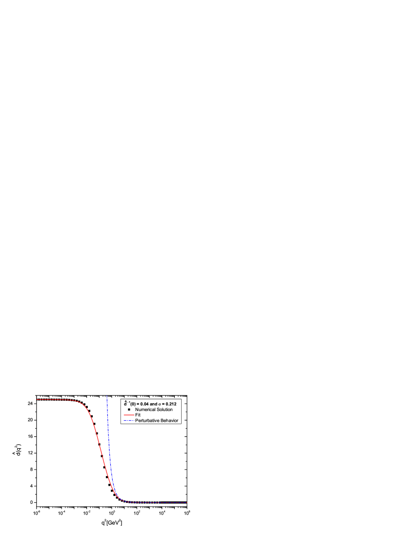
Figure 6: The black dots represent the numerical solution for ${\widehat{d}}(q^{2})$ obtained for the choice ${\widehat{d}}^{\,-1}(0)=0.04\;\mbox{GeV}^{\,2}$, $\sigma=0.212$ and $\gamma=0.941$. The continuous red line is the fit of Eq.(3.17), setting $\rho_{2}=-3.208$ and $m^{2}_{0}=0.45\,\mbox{GeV}^{\,2}$. These curves are obtained fixing ${\widehat{d}}^{\,-1}(0)=0.04\;\mbox{GeV}^{\,2}$, $\sigma=0.212$ and $\gamma=0.941$. The dashed blue line is the one-loop perturbative behavior.

The dynamical mass, $m^{2}(q^{2})$, and the running charge, $\alpha(q^{2})={\overline{g}}^{2}_{{{\scriptscriptstyle\rm NP}}}(q^{2})/4\pi$, corresponding to the numerical solution presented on the Fig. 6, are shown in Figs. 7 and 8, respectively.

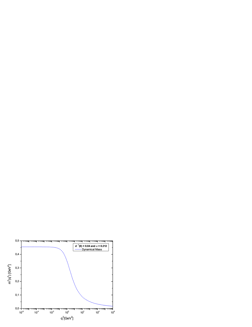
Figure 7: The dynamical mass, $m^{2}(q^{2})$, corresponding to the solution of Fig. 6.

Figure 8: The running charge, $\alpha(q^{2})={\overline{g}}^{2}_{{{\scriptscriptstyle\rm NP}}}(q^{2})/4\pi$ corresponding to the solution of Fig. 6.

In fact, in all cases studied, $\rho_{\,1}$ was fixed to the value $\rho_{\,1}=4$, which was found to minimize the $\chi^{2}$ of the corresponding fits. Therefore, the unique free parameter is $\rho_{\,2}$, since the value of $m^{2}_{0}$ can be written in terms of $\rho_{\,2}$, simply by setting $q^{2}=0$, in Eq.(3.17), i.e.,

$${\widehat{d}}^{\,-1}(0)=\tilde{b}\,m^{2}_{0}\ln\left(\frac{f(0,m^{2}_{0})}{\Lambda^{2}}\right)\,,$$ (5.6)

where

$$f(0,m^{2}_{0})=(4+\rho_{\,2})\,m^{2}_{0}\,.$$ (5.7)

Thus, the value of the IR fixed point of the running coupling is determined by the value assumed by $f(0,m^{2}_{0})$, since

$${\overline{g}}^{\,-2}_{{{\scriptscriptstyle\rm NP}}}(0)=\tilde{b}\ln\left[\frac{(4+\rho_{\,2})\,m^{2}_{0}}{\Lambda^{2}}\right]\,,$$ (5.8)

Obviously, the maximum value obtained for ${\overline{g}}^{2}_{{{\scriptscriptstyle\rm NP}}}(0)$, is the one that minimizes $(4+\rho_{\,2})\,m^{2}_{0}$ and, at same time, keeps it bigger than $\Lambda^{2}$, in order to avoid the appearance of a shifted version of the Landau pole.

Note that the term proportional to $\rho_{\,2}$ in (5.4) is necessary for optimizing the fit for the range of momenta $q^{2}\in[0.01\;\mbox{GeV}^{\,2},2\;\mbox{GeV}^{\,2}]$, i.e. the region where ${\widehat{d}}(q^{2})$ falls down rapidly. If we were to set $\rho_{\,2}=0$ in Eq.(5.4) we would recover automatically the solution proposed in Cornwall:1982zr ; however, such a choice would not correspond to the best possible fit: our numerical solution requires bigger values for the coupling ${\overline{g}}^{2}_{{{\scriptscriptstyle\rm NP}}}(q^{2})$, and therefore, $\rho_{\,2}$ assumes negative values, as can be observed on Fig. 6, where found that $\rho_{\,2}=-3.208$.

It is important to mention that other functional forms for $f(q^{2},m^{2}(q^{2}))$ were also tried; although some of them could fit ${\widehat{d}}(q^{2})$ well, they have been discarded due to the appearance, at some scale, of an undesired “bump” in the behavior of ${\overline{g}}^{2}_{{{\scriptscriptstyle\rm NP}}}(q^{2})$. In others words, we have required that ${\overline{g}}^{2}_{{{\scriptscriptstyle\rm NP}}}(q^{2})$ should be a monotonically decreasing function of $q^{2}$.

In Fig. 9 we plot a series of numerical solution obtained by fixing different values for ${\widehat{d}}^{\,-1}(0)$. All these solutions have been subjected to the constraint imposed by Eq.(5.2), and their corresponding values for $\sigma$ are reported in the inserted legend. Observe that they all behave like constants until practically the same scale of $0.01\;\mbox{GeV}^{\,2}$ (the “freezing” plateau), then they converge down to a common value at around $1\;\mbox{GeV}^{\,2}$, beyond which they start to develop the known perturbative behavior.

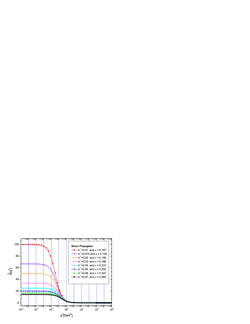
Figure 9: Results for ${\widehat{d}}(q^{2})$ for various values of ${\widehat{d}}^{\,-1}(0)$ (all in $\;\mbox{GeV}^{\,2}$), together with the respective values for $\sigma$, obtained from the constraint of Eq.(5.2).

The running charges, $\alpha(q^{2})$, for each solution presented in Fig. 9, are displayed on Fig. 10. Observe that as the value of ${\widehat{d}}^{\,-1}(0)$ decreases, the value of the infrared fixed point of the running coupling, $\alpha(0)$, increases. Accordingly, from Fig. 9 and Fig. 10, we can conclude that, if smaller values of $\sigma$ were to be favored by QCD, the freezing of the running coupling would occur at higher values. It should also be noted that the values of $\alpha(0)$ found here tend to be slightly more elevated compared to those of Cornwall:1982zr (for the same value of $m^{2}_{0}$).

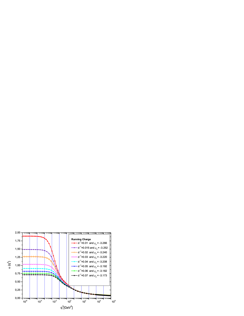
Figure 10: We plot the correspondent running charge, $\alpha(q^{2})$, for the gluon propagator presented on Fig. 9. Clearly, we can see as we decrease the values of ${\widehat{d}}^{\,-1}(0)$ the infrared fixed point, $\alpha(0)$, becomes bigger.

In addition we analyze the dependence of the ratio $m_{0}/\Lambda$ on $\sigma$, extracted from Eq.(5.6). This dependence is shown in Fig. 11, corresponding to the cases presented in Fig. 9. We observe that as we increase the value of $\sigma$, namely the sum of the coefficients of the massless pole terms appearing in the three gluon vertex, the ratio $m_{0}/\Lambda$ grows exponentially as

$$\frac{m_{0}}{\Lambda}=A_{1}\exp\left(\frac{\sigma}{t_{1}}\right)+y_{0}\,,$$ (5.9)

with $A_{1}=0.775$, $t_{1}=0.25$ and $y_{0}=0.436$.

At this point it is natural to ask by how much these results would change if we were to turn on again $c_{2}$ in Eq.(5.3). We have examined values of $c_{2}$ comparable to those used for $\sigma$, i.e. we exclude the possibility that the typically small values of $\sigma$ are a result of a very fine-tuned cancellation between large $c_{1}$ and $c_{2}$, opposite in sign. It turns out that, for all previous cases studied, the effect of including non-vanishing $c_{2}$’s in Eq.(5.3) is less than $3\%$, a fact that justifies their omission.

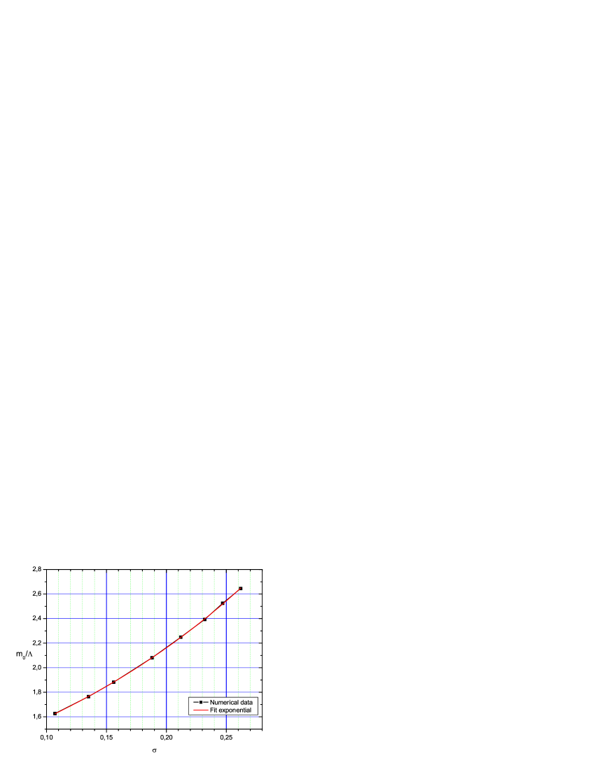
Figure 11: The ratio $m_{0}/\Lambda$ as function of the parameter $\sigma$. The increase is exponential, given by Eq.(5.9).

V.2 Non-canonical solutions

As we decrease ${\widehat{d}}^{\,-1}(0)$, it becomes increasingly difficult to fit the numerical solution obtained from Eq. (5.1) using the expressions given in (3.17), (5.4), and (5.5). In particular, for solutions with ${\widehat{d}}^{\,-1}(0)<0.01\;\mbox{GeV}^{\,2}$, the discrepancy is relatively large, especially in the intermediate region. We will denote such non-canonical solutions by ${\widehat{d}}_{\rm\,N}(q^{2})$. A typical numerical solution is shown by the curve composed by black squares in Fig. 12. It is important to emphasize that, although the form of Eq.(3.17) is not suited for fitting the entire momentum range, one may use it for describing a partial region, i.e. $q^{2}\in[0.2\,\mbox{GeV}^{\,2},\Lambda_{\rm{UV}}]$, as showed by the line+circle curve on Fig. 12, where we clearly see a quantitative agreement between both curves. This observation is related to the discussion following Eq.(3.25), allowing us to use the same regularization procedure as in (5.2).

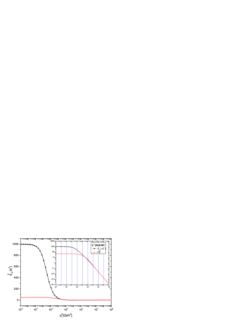
Figure 12: The black square points represent the numerical solution for the RGI quantity ${\widehat{d}}(q^{2})=g^{2}{\widehat{\Delta}}(q^{2})$, when we fixed ${\widehat{d}}^{\,-1}(0)=0.001\;\mbox{GeV}^{\,2}$ and $\sigma=7.65\times 10^{\,-3}$. The red line + circle curve is the fit given by Eq.(3.17), setting $\rho_{2}=-\pi$ and $m^{2}_{0}=0.304\;\mbox{GeV}^{\,2}$. The small plot is the same graph on log-log scale.

To see this, let us denote by ${\widehat{d}}_{\rm\,C}(z)$ the canonical solution that provides the best fit to a given ${\widehat{d}}_{\rm\,N}(z)$; then write ${\widehat{d}}_{\rm\,N}(z)=[{\widehat{d}}_{\rm\,N}(z)-{\widehat{d}}_{\rm\,C}(z)]+{\widehat{d}}_{\rm\,C}(z)$, and substitute into Eq.(5.2), to obtain

$${\widehat{d}}^{\,-1}(0)={\tilde{b}}\sigma\bigg{[}{\widehat{d}}\to{\widehat{d}}_{\rm\,C}\bigg{]}-{\tilde{b}}\sigma\int_{0}^{\infty}\!\!dz\;z\frac{{\widehat{d}_{\rm\,N}}(z)-{\widehat{d}}_{\rm\,C}(z)}{\bar{g}^{2}(z)},$$ (5.10)

The first term on the RHS of Eq.(5.10) is simply the RHS of Eq.(5.2), with ${\widehat{d}}\to{\widehat{d}}_{\rm\,C}$; it clearly converges, since ${\widehat{d}}_{\rm\,C}$ is (by construction) a canonical solution. The second term receives an appreciable contribution only in the low momenta region, i.e. from $0$ to $0.2\;\mbox{GeV}^{\,2}$, vanishing very rapidly in the UV, due to the perfect agreement found between both curves for the range $[0.2\;\mbox{GeV}^{\,2},\Lambda_{\rm{UV}}]$.

Other non-canonical solutions with different ${\widehat{d}}^{\,-1}(0)$ are plotted on Fig. 13, and their respective values of $\sigma$ are reported in the legend. Notice that, as the value of ${\widehat{d}}(0)$ increases, the IR plateau becomes narrower.

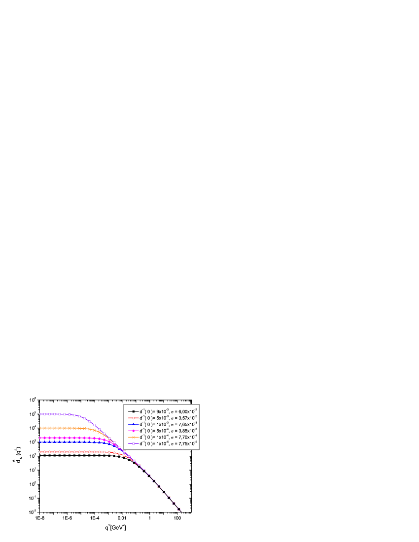
Figure 13: Results for ${\widehat{d}}(q^{2})$ fixing different values for ${\widehat{d}}^{\,-1}(0)$ (all in $\mbox{GeV}^{\,2}$) in a log-log plot. All solutions presented satisfy the condition given by Eq.(5.10). Their respective values for $\sigma$ are described on its legend.

Finally, the dependence of ${\widehat{d}}^{\,-1}(0)$ on $\sigma$ for all cases presented here is shown on Fig. 14, in a log-log plot. The results clearly show a linear behavior for smaller values of ${\widehat{d}}^{\,-1}(0)$, whereas for values of ${\widehat{d}}^{\,-1}(0)\geq 0.01\;\mbox{GeV}^{\,2}$ the growth is exponential.

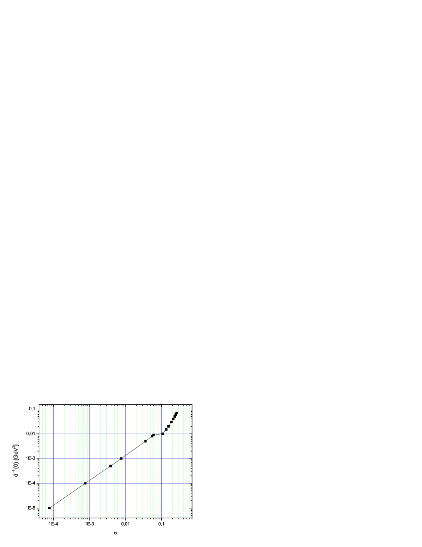
Figure 14: ${\widehat{d}}^{\,-1}(0)$ as function of $\sigma$.

VI Discussion and Conclusions

In this article we have taken a closer look at various issues relevant to the study of gluon mass generation through SD equations. The emphasis of our analysis has focused on the following points: (i) The gauge-invariant truncation scheme based on the PT-BFM formalism, and the possibility it offers in implementing a self-consistent first approximation, omitting ghost contributions without compromising the transversality of the gluon self-energy. (ii) The necessity of introducing massless poles in the form of the vertex used in the SD equation, and the role of the seagull graph in enforcing transversality (iii) A method for regulating the resulting seagull-type integrals based on dimensional regularization, and the asymptotic properties that the solutions must display in the UV in order for this regularization to work. (iv) We have derived a linearized version of the SD equation that originates from the one-loop dressed approximation, in the absence of ghost loops. (v) We have introduced a phenomenological form for the three-gluon vertex, containing massless poles associated with two different tensorial structures. (vi) The resulting equation has been solved numerically and two types of qualitatively distinct solutions have been found.

It should be obvious from the present work that the role of the three-gluon vertex is absolutely central; in particular, the question of whether or not it contains massless poles is a determining factor when looking for finite solutions. As we have mentioned already, the form of the vertex employed here attempts to capture some of the main features, such as the impact of the poles, and the possible interplay between poles originating from different Lorentz structures (see discussion after (4.14)). Needless to say, an in-depth study of the form of the vertex is indispensable for further substantiating the appearance of IR-finite solutions. At the moment we only have indications from the study of SD equation and lattice simulations (albeit for the three-gluon vertex in the conventional Landau gauge) that the IR behavior is indeed singular. In addition, one must explore the possibility of improving the gauge-technique inspired Ansätze employed for the vertex, in the spirit of King:1982mk , in an attempt to correctly incorporate the required asymptotic behavior into the SD equation (see Sec. III). Given the rich tensorial structure of the three-gluon vertex Binger:2006sj , such a task is expected to be technically rather demanding.

It would be interesting to further scrutinize the viability of the new class of solutions encountered in Sec. V. Such solutions are particularly interesting, because they could in principle overcome a well-known difficulty related to the breaking of chiral symmetry. Specifically, the class of solutions displaying freezing, when inserted into standard forms of the gap-equation for the quarks, are not able to trigger non-trivial solution, because they do no reach high enough values in the IR to overcome the critical coupling Papavassiliou:1991hx . Instead, the new type of solutions rises sharply in the deep IR, reaching values that could in principle break chiral symmetry, while for intermediate IR momenta it coincides with a canonical massive type of solution, that seems to be favored by phenomenology Aguilar:2002tc . Of course, it could well happen that these solutions are particular to the linearized equation, and do not survive a non-linear analysis.

In recent years the picture that has emerged through the study of SD equations in the conventional Landau gauge is characterized by the so-called “ghost dominance” vonSmekal:1997is ; Atkinson:1997tu . In particular, the gluon self-energy has the form $\Delta_{\,\mu\nu}(q^{2})=\Delta(q^{2}){\rm P}_{\mu\nu}(q)$, with $\Delta(q^{2})=Z(q^{2})/q^{2}$, and the ghost propagator is $D(q^{2})=-C(q^{2})/q^{2}$. Assuming that the dressed ghost-gluon vertex is finite in the IR, the SD equations yields for $q^{2}\rightarrow 0$, $C(q^{2})=A\,q^{-2\kappa}$, $Z(q^{2})=B\,q^{\,4\kappa}$, where the constants $A$ and $B$ depend on $\kappa$. The value of $\kappa$ depends on the details of the dressing of the gluon-ghost vertex at small momenta; SD and lattice studies seem to restrict it within the range $0.5\leq\kappa<0.6$. For the special value $\kappa=0.5$ one obtains a finite gluon propagator, $\Delta(0)=B$, whereas the ghost propagator diverges as $D(q^{2})\to-A(q^{2})^{-3/2}$. In addition, by virtue of the identity $\tilde{Z_{1}}=Z_{g}Z_{3}^{1/2}\tilde{Z_{3}}=1$, valid in the Landau gauge, where $\tilde{Z_{1}}$, $Z_{g}$, $Z_{3}$ and $\tilde{Z_{3}}$ are the gluon-ghost vertex, coupling, gluon and ghost renormalization constants respectively, one concludes that the product $g^{2}Z(q^{2})C^{2}(q^{2})$ is RG-invariant, and can be adopted as a definition of the non-perturbative running coupling, i.e. $\alpha(q^{2})=(g^{2}/4\pi)Z(q^{2})C^{2}(q^{2})$. Then it is clear that the $\alpha(q^{2})$ so defined has an IR fixed point, $\alpha(0)=(g^{2}/4\pi)A^{2}\,B\,$, regardless of the value of $\kappa$. The actual value of $\alpha(0)$ depends on $\kappa$, through the implicit dependence of $A$ and $B$ on it; for values of $0.5\leq\kappa<0.6$, one obtains $2.5\leq\alpha(0)<3$. Evidently, the (dimensionfull) RG-invariant quantity $\widehat{d}(q^{2})$ studied in this article displays a qualitatively similar behavior to that found for the (dimensionless) running coupling in the “ghost-dominance” picture, namely IR finiteness. Therefore, despite the difference in the intermediate steps and the terminology employed, the physics captured by both pictures appears to be compatible. Notice also that, from the practical point of view, the method presented here has the advantage of setting up a SD equation directly for the RG-invariant object of interest; thus, the result obtained does not depend on the exactness with which a subtle cancellation in the ratio of two quantities, one tending to zero and one to infinity, is realized. This last comment may be particularly relevant in the context of lattice simulations, where the above ratio is studied numerically; clearly, a small deviation from the exact cancellation (due to residual volume dependences, for instance) may lead to serious qualitative discrepancies. It is also important to mention that, whereas the confinement mechanism within the “ghost-dominance” description is attributed to the divergence of the ghost propagator Gribov:1977wm , in the picture where the gluon is massive the origin of confinement is the condensation of vortices Cornwall:1979hz ; Zakharov:2005cg . Actually, recent investigations advocate interesting connections between the center-vortex picture and the Gribov-horizon scenario Gattnar:2004bf .

As mentioned in the Introduction, in the PT-BFM scheme the omission of the ghost loop does not interfere with gauge-invariance, but it might alter the actual form of the gluon self-energy. Therefore, the study of the gluon-ghost system should be eventually considered. Of particular relevance in such a study is the nature of the gluon-ghost vertices involved; in fact, in the PT-BFM scheme there will be two such vertices: ${\widetilde{{\rm I}\Gamma}}_{\nu}$, appearing in Fig. 3, and ${{\rm I}\Gamma}_{\beta}$, which will appear in the SD equation for the ghost propagator. The IR behavior of ${{\rm I}\Gamma}_{\beta}$ (in the Landau gauge) is currently under investigation on the lattice Bloch:2003sk ; it would clearly be important to settle the issue of whether it is divergent or finite.

Last but not least, the theoretical situation concerning the SD equations within the PT-BFM scheme merits further intense scrutiny. First of all, the correspondence between the PT and BFM has been established perturbatively to all orders, but no analogous proof exists non-perturbatively, i.e. at the level of the SD equations themselves. In this article we have assumed that the PT-BFM correspondence persists non-perturbatively. A preliminary study in a simplified context (scalar QED) fully corroborates this assumption sqed ; however, the actual realization is highly non-trivial, and its generalization to QCD deserves a thorough analysis. In the same context, the consequences of the second crucial ingredient, namely the substitution of quantum quantities by background ones inside the loops, are virtually unexplored. One must study in detail, preferably in the context of the toy model mentioned above, the viability and self-consistency of this procedure. We hope to be able to undertake some of these tasks in the near future.

*

Appendix A Feynman rules in the BFM

In this Appendix we list for completeness the Feynman rules appearing in Abbott:1980hw .

$$-i\left[g_{\mu\nu}-(1-\xi_{Q})\frac{k_{\mu}k_{\nu}}{k^{2}}\right]\frac{\delta^{ab}}{k^{2}+i\epsilon}$$ (A-1)

$$\frac{i\delta^{ab}}{k^{2}+i\epsilon}$$ (A-2)

$$gf^{abc}\left[\left(p_{1}-q\right)_{\nu}g_{\mu\alpha}+\left(q-p_{2}\right)_{\mu}g_{\nu\alpha}+\left(p_{2}-p_{1}\right)_{\alpha}g_{\mu\nu}\right]$$ (A-3)

$$gf^{abc}\left[\left(p_{1}-q+\frac{1}{\xi_{Q}}p_{2}\right)_{\nu}g_{\mu\alpha}+\left(q-p_{2}-\frac{1}{\xi_{Q}}p_{1}\right)_{\mu}g_{\nu\alpha}+\left(p_{2}-p_{1}\right)_{\alpha}g_{\mu\nu}\right]\!\!$$ (A-4)

$\displaystyle-ig^{2}\bigg{[}f^{abx}f^{xcd}\left(g_{\mu\alpha}g_{\nu\beta}-g_{\mu\beta}g_{\nu\alpha}\right)\bigg{.}$ $\displaystyle\bigg{.}+f^{adx}f^{xbc}\left(g_{\mu\nu}g_{\alpha\beta}-g_{\mu\alpha}g_{\nu\beta}\right)\bigg{.}$ $\displaystyle+\bigg{.}f^{acx}f^{xbd}\left(g_{\mu\nu}g_{\alpha\beta}-g_{\mu\beta}g_{\nu\alpha}\right)\bigg{]}$ (A-5)

$\displaystyle-ig^{2}\bigg{[}f^{abx}f^{xcd}\left(g_{\mu\alpha}g_{\nu\beta}-g_{\mu\beta}g_{\nu\alpha}+\frac{1}{\xi_{Q}}g_{\mu\nu}g_{\alpha\beta}\right)\bigg{.}$ $\displaystyle\bigg{.}+f^{adx}f^{xbc}\left(g_{\mu\nu}g_{\alpha\beta}-g_{\mu\alpha}g_{\nu\beta}-\frac{1}{\xi_{Q}}g_{\mu\beta}g_{\nu\alpha}\right)\bigg{.}$ $\displaystyle+\bigg{.}f^{acx}f^{xbd}\left(g_{\mu\nu}g_{\alpha\beta}-g_{\mu\beta}g_{\nu\alpha}\right)\bigg{]}$ (A-6)

$$-gf^{abc}(p+q)_{\mu}$$ (A-7)

$$-gf^{abc}p_{\mu}$$ (A-8)

	$$-ig^{2}f^{acx}f^{xdb}g_{\mu\nu}$$ (A-9)
	$$-ig^{2}g_{\mu\nu}\left(f^{acx}f^{xdb}+f^{adx}f^{xcb}\right)$$ (A-10)

References

- (1) W. J. Marciano and H. Pagels, Phys. Rept. 36, 137 (1978).
- (2) See, for example, K. D. Lane, Phys. Rev. D 10, 2605 (1974); H. Pagels, Phys. Rev. D 19, 3080 (1979); D. Atkinson and P. W. Johnson, Phys. Rev. D 37 (1988) 2290; C. D. Roberts and B. H. McKellar, Phys. Rev. D 41 (1990) 672.
- (3) J. M. Cornwall, in Deeper Pathways in High-Energy Physics, edited by B. Kursunoglu, A. Perlmutter, and L. Scott (Plenum, New York, 1977), p 683.
- (4) J. M. Cornwall, Nucl. Phys. B 157, 392 (1979).
- (5) G. Parisi and R. Petronzio, Phys. Lett. B 94, 51 (1980);
- (6) B. Berg, Phys. Lett. B 97, 401 (1980).
- (7) G. Bhanot and C. Rebbi, Nucl. Phys. B 180, 469 (1981).
- (8) C. W. Bernard, Phys. Lett. B 108, 431 (1982).
- (9) For related works, see J. Smit, Phys. Rev. D 10, 2473 (1974); R. Fukuda, Phys. Lett. B 73, 33 (1978) [Erratum-ibid. B 74, 433 (1978)]. V. P. Gusynin and V. A. Miransky, Phys. Lett. B 76, 585 (1978).
- (10) M. A. Shifman, A. I. Vainshtein and V. I. Zakharov, Nucl. Phys. B 147, 448 (1979); Nucl. Phys. B 147, 385 (1979).
- (11) J. M. Cornwall, Phys. Rev. D 26, 1453 (1982).
- (12) J. M. Cornwall and J. Papavassiliou, Phys. Rev. D 40, 3474 (1989).
- (13) J. Papavassiliou, Phys. Rev. D 41, 3179 (1990).
- (14) D. Binosi and J. Papavassiliou, Phys. Rev. D 66, 111901 (2002); J. Phys. G 30, 203 (2004).
- (15) C. W. Bernard, Nucl. Phys. B 219, 341 (1983); J. F. Donoghue, Phys. Rev. D 29, 2559 (1984); M. H. Thoma and H. J. Mang, Z. Phys. C 44, 349 (1989); E. Bagan and M. R. Pennington, Phys. Lett. B 220, 453 (1989); U. Habel, R. Konning, H. G. Reusch, M. Stingl and S. Wigard, Z. Phys. A 336, 423 (1990); Z. Phys. A 336 (1990) 435.
- (16) M. Lavelle, Phys. Rev. D 44, 26 (1991); M. Consoli and J. H. Field, Phys. Rev. D 49, 1293 (1994); A. C. Mattingly and P. M. Stevenson, Phys. Rev. Lett. 69, 1320 (1992); J. E. Shrauner, J. Phys. G 19, 979 (1993); F. J. Yndurain, Phys. Lett. B 345 (1995) 524; A. Szczepaniak, E. S. Swanson, C. R. Ji and S. R. Cotanch, Phys. Rev. Lett. 76, 2011 (1996).
- (17) K. I. Kondo, Phys. Lett. B 514, 335 (2001); K. I. Kondo, T. Murakami, T. Shinohara and T. Imai, Phys. Rev. D 65, 085034 (2002); K. I. Kondo,arXiv:hep-th/0609166.
- (18) J. C. R. Bloch, Few Body Syst. 33, 111 (2003).
- (19) A. C. Aguilar and A. A. Natale, JHEP 0408, 057 (2004).
- (20) D. Dudal, J. A. Gracey, V. E. R. Lemes, M. S. Sarandy, R. F. Sobreiro, S. P. Sorella and H. Verschelde, Phys. Rev. D 70, 114038 (2004); D. Dudal, H. Verschelde, J. A. Gracey, V. E. R. Lemes, M. S. Sarandy, R. F. Sobreiro and S. P. Sorella, JHEP 0401, 044 (2004).
- (21) S. P. Sorella, Annals Phys. 321, 1747 (2006).
- (22) C. Alexandrou, P. de Forcrand and E. Follana, Phys. Rev. D 63, 094504 (2001); Phys. Rev. D 65, 117502 (2002); Phys. Rev. D 65, 114508 (2002).
- (23) F. D. R. Bonnet, P. O. Bowman, D. B. Leinweber and A. G. Williams, Phys. Rev. D 62, 051501 (2000); F. D. R. Bonnet, P. O. Bowman, D. B. Leinweber, A. G. Williams and J. M. Zanotti, Phys. Rev. D 64, 034501 (2001).
- (24) A. Sternbeck, E. M. Ilgenfritz, M. Mueller-Preussker and A. Schiller, Phys. Rev. D 72, 014507 (2005); P. J. Silva and O. Oliveira, arXiv:hep-lat/0511043; Ph. Boucaud et al., arXiv:hep-ph/0507104; Ph. Boucaud et al., JHEP 0606, 001 (2006); A. Cucchieri and T. Mendes, Phys. Rev. D 73, 071502 (2006).
- (25) F. Halzen, G. I. Krein and A. A. Natale, Phys. Rev. D 47, 295 (1993); M. B. Gay Ducati, F. Halzen and A. A. Natale, Phys. Rev. D 48, 2324 (1993); J. R. Cudell and B. U. Nguyen, Nucl. Phys. B 420, 669 (1994); A. Donnachie and P. V. Landshoff, Phys. Lett. B 387, 637 (1996).
- (26) A. Mihara and A. A. Natale, Phys. Lett. B 482, 378 (2000); J. H. Field, Phys. Rev. D 66, 013013 (2002); F. Cano and J. M. Laget, Phys. Rev. D 65, 074022 (2002); R. Enberg, G. Ingelman and L. Motyka, Phys. Lett. B 524, 273 (2002); M. B. Gay Ducati and W. K. Sauter, Phys. Rev. D 67, 014014 (2003); W. S. Hou and G. G. Wong, Phys. Rev. D 67, 034003 (2003); E. G. S. Luna, A. F. Martini, M. J. Menon, A. Mihara and A. A. Natale, Phys. Rev. D 72, 034019 (2005); E. G. S. Luna and A. A. Natale, Phys. Rev. D 73, 074019 (2006); E. G. S. Luna, A. A. Natale and C. M. Zanetti, arXiv:hep-ph/0605338; E. G. S. Luna, arXiv:hep-ph/0608091.
- (27) A. C. Mattingly and P. M. Stevenson, Phys. Rev. D 49, 437 (1994).
- (28) Y. L. Dokshitzer, G. Marchesini and B. R. Webber, Nucl. Phys. B 469 (1996) 93;
- (29) L. von Smekal, R. Alkofer and A. Hauck, Phys. Rev. Lett. 79, 3591 (1997).
- (30) A. M. Badalian and V. L. Morgunov, Phys. Rev. D 60, 116008 (1999).
- (31) A. C. Aguilar, A. A. Natale and P. S. Rodrigues da Silva, Phys. Rev. Lett. 90, 152001 (2003); A. C. Aguilar, A. Mihara and A. A. Natale, Phys. Rev. D 65, 054011 (2002); Int. J. Mod. Phys. A 19 (2004) 249.
- (32) S. J. Brodsky, S. Menke, C. Merino and J. Rathsman, Phys. Rev. D 67, 055008 (2003); S. J. Brodsky, Fizika B 13, 91 (2004).
- (33) M. Baldicchi and G. M. Prosperi, Phys. Rev. D 66, 074008 (2002).
- (34) G. Grunberg, Phys. Rev. D 29, 2315 (1984); Phys. Rev. D 73, 091901 (2006).
- (35) H. Gies, Phys. Rev. D 66, 025006 (2002).
- (36) D. V. Shirkov and I. L. Solovtsov, Phys. Rev. Lett. 79, 1209 (1997); A. V. Nesterenko and J. Papavassiliou, Phys. Rev. D 71, 016009 (2005); A. P. Bakulev, S. V. Mikhailov and N. G. Stefanis, Phys. Rev. D 72, 074014 (2005) [Erratum-ibid. D 72, 119908 (2005)].
- (37) J. A. Gracey, JHEP 0605, 052 (2006).
- (38) For a recent comprehensive review see, G. M. Prosperi, M. Raciti and C. Simolo, arXiv:hep-ph/0607209.
- (39) D. Binosi and J. Papavassiliou, Phys. Rev. D 66, 025024 (2002)
- (40) A. Denner, G. Weiglein and S. Dittmaier, Phys. Lett. B 333, 420 (1994); S. Hashimoto, J. Kodaira, Y. Yasui and K. Sasaki, Phys. Rev. D 50, 7066 (1994); J. Papavassiliou, Phys. Rev. D 51, 856 (1995); A. Pilaftsis, Nucl. Phys. B 487, 467 (1997).
- (41) J. Papavassiliou, Phys. Rev. Lett. 84, 2782 (2000); Phys. Rev. D 62, 045006 (2000).
- (42) B. S. Dewitt, Phys. Rev. 162, 1195 (1967); J. Honerkamp, Nucl. Phys. B 48, 269 (1972); R. E. Kallosh, Nucl. Phys. B 78, 293 (1974); H. Kluberg-Stern and J. B. Zuber, Phys. Rev. D 12, 482 (1975); G. ’t Hooft, In *Karpacz 1975, Proceedings, Acta Universitatis Wratislaviensis No.368, Vol.1*, Wroclaw 1976, 345-369; S. Weinberg, Phys. Lett. B 91, 51 (1980).
- (43) L. F. Abbott, Nucl. Phys. B 185, 189 (1981).
- (44) P. Gambino and P. A. Grassi, Phys. Rev. D 62, 076002 (2000); P. A. Grassi, T. Hurth and M. Steinhauser, Annals Phys. 288, 197 (2001).
- (45) R. Jackiw and K. Johnson, Phys. Rev. D 8, 2386 (1973); J. M. Cornwall and R. E. Norton, Phys. Rev. D 8 (1973) 3338; E. Eichten and F. Feinberg, Phys. Rev. D 10, 3254 (1974); J. M. Cornwall, R. Jackiw and E. Tomboulis, Phys. Rev. D 10, 2428 (1974).
- (46) T. Kunimasa and T. Goto, Prog. Theor. Phys. 37, 452 (1967); A. A. Slavnov, Theor. Math. Phys. 10, 305 (1972); J. M. Cornwall, Phys. Rev. D 10, 500 (1974).
- (47) J. R. Forshaw, J. Papavassiliou and C. Parrinello, Phys. Rev. D 59, 074008 (1999).
- (48) A. Salam, Phys. Rev. 130, 1287 (1963); R. Delbourgo and A. Salam, Phys. Rev. 135 (1964) 1398B; R. Delbourgo and P. West, J. Phys. A 10, 1049 (1977); R. Delbourgo, Nuovo Cim. A 49, 484 (1979).
- (49) C. Becchi, A. Rouet and R. Stora, Annals Phys. 98, 287 (1976); I. V. Tyutin, Lebedev Institute Report, 75-39.
- (50) N. J. Watson, Nucl. Phys. B 494, 388 (1997).
- (51) D. Binosi and J. Papavassiliou, Nucl. Phys. Proc. Suppl. 121, 281 (2003)
- (52) S. Weinberg, The Quantum Theory of Fields (Cambridge University Press, New York, 1996), Vol. II.
- (53) R. B. Sohn, Nucl. Phys. B 273, 468 (1986); A. Hadicke, JENA-N-88-19.
- (54) J. Papavassiliou, Phys. Rev. D 47, 4728 (1993).
- (55) I. A. Batalin and G. A. Vilkovisky, Phys. Lett. B 69 (1977) 309; Phys. Rev. D 28 (1983) 2567 [Erratum-ibid. D 30 (1984) 508].
- (56) P. Pascual and R. Tarrach, QCD: Renormalization for the Practitioner (Springer-Verlag, Heidelberg, 1984).
- (57) U. Bar-Gadda, Nucl. Phys. B 163, 312 (1980).
- (58) J. S. Ball and T. W. Chiu, Phys. Rev. D 22, 2550 (1980) [Erratum-ibid. D 23, 3085 (1981)].
- (59) P. A. Grassi, T. Hurth and A. Quadri, Phys. Rev. D 70, 105014 (2004).
- (60) For example, in M. Baker, J. S. Ball and F. Zachariasen, Nucl. Phys. B 186, 531 (1981); Nucl. Phys. B 186, 560 (1981), no massless poles were introduced in the vertex, thus explicitly excluding the possibility of gluon mass generation.
- (61) It should be clear that the seagull contribution cannot be “projected out” and discarded, since it forms part of the scalar cofactor multiplying the projection operator . The only reason why this can be done some times in the literature is because the transversality of the answer has been compromised at an earlier stage, due to some incomplete approximation.
- (62) J. E. King, Phys. Rev. D 27, 1821 (1983); B. J. Haeri, Phys. Rev. D 38, 3799 (1988).
- (63) J. M. Cornwall and W. S. Hou, Phys. Rev. D 34, 585 (1986).
- (64) See, Eq.(4.2.6) in J.C.Collins, “Renormalization”, Cambrigde University Press, Cambridge, 1984.
- (65) See, for example, J. M. Cornwall and R. C. Shellard, Phys. Rev. D 18, 1216 (1978).
- (66) Some of the general assumptions on have been discussed in Cornwall:1982zr . The issue of reconciling a positive definite spectral density with asymptotic freedom has been studied in J. Frenkel and J. C. Taylor, Nucl. Phys. B 109, 439 (1976) [Erratum-ibid. B 155, 544 (1979)]. For an interesting discussion, see S. Catani and E. D’Emilio, Fortsch. Phys. 41 (1993) 261.
- (67) In the derivation of the second identity we have used that Cornwall:1982zr .
- (68) M. Binger and S. J. Brodsky, arXiv:hep-ph/0602199.
- (69) J. Papavassiliou and J. M. Cornwall, Phys. Rev. D 44, 1285 (1991).
- (70) D. Atkinson and J. C. R. Bloch, Phys. Rev. D 58, 094036 (1998); R. Alkofer and L. von Smekal, Phys. Rept. 353, 281 (2001); J. C. R. Bloch, Phys. Rev. D 64, 116011 (2001); C. Lerche and L. von Smekal, Phys. Rev. D 65, 125006 (2002); R. Alkofer, C. S. Fischer and F. J. Llanes-Estrada, Phys. Lett. B 611, 279 (2005); C. S. Fischer, J. Phys. G 32, R253 (2006).
- (71) V. N. Gribov, Nucl. Phys. B 139, 1 (1978); T. Kugo and I. Ojima, Prog. Theor. Phys. Suppl. 66, 1 (1979); D. Zwanziger, Nucl. Phys. B 364, 127 (1991); Nucl. Phys. B 399, 477 (1993); R. Alkofer, C. S. Fischer and F. J. Llanes-Estrada, arXiv:hep-ph/0607293.
- (72) For a similar point of view, see V. I. Zakharov, arXiv:hep-ph/0509114, and references therein.
- (73) J. Gattnar, K. Langfeld and H. Reinhardt, Phys. Rev. Lett. 93, 061601 (2004); J. Greensite, S. Olejnik and D. Zwanziger, JHEP 0505, 070 (2005).
- (74) J. C. R. Bloch, A. Cucchieri, K. Langfeld and T. Mendes, Nucl. Phys. B 687, 76 (2004); A. Cucchieri, T. Mendes and A. Mihara, JHEP 0412, 012 (2004); A. Sternbeck, E. M. Ilgenfritz, M. Muller-Preussker and A. Schiller, Nucl. Phys. Proc. Suppl. 153, 185 (2006).
- (75) D. Binosi and J. Papavassiliou, in preparation.