LHC String Phenomenology

Abstract

We argue that it is possible to address the deeper LHC Inverse Problem, to gain insight into the underlying theory from LHC signatures of new physics. We propose a technique which may allow us to distinguish among, and favor or disfavor, various classes of underlying theoretical constructions using (assumed) new physics signals at the LHC. We think that this can be done with limited data $(5-10\,fb^{-1})$, and improved with more data. This is because of two reasons – a) it is possible in many cases to reliably go from (semi)realistic microscopic string constructions to the space of experimental observables, say, LHC signatures. b) The patterns of signatures at the LHC are sensitive to the structure of the underlying theoretical constructions. We illustrate our approach by analyzing two promising classes of string compactifications along with six other string-motivated constructions. Even though these constructions are not complete, they illustrate the point we want to emphasize. We think that using this technique effectively over time can eventually help us to meaningfully connect experimental data to microscopic theory.

I Introduction

The start of the LHC will usher in a new era of particle physics. Hopefully, physics beyond the standard model will be discovered. Many possibilities for new physics have been proposed and their phenomenological implications have been studied in detail. When the LHC starts accumulating data, one would like to answer the following little studied question – Assuming a signal for physics beyond the standard model, how can one determine the nature of new physics from LHC data? This question, the so-called “LHC Inverse Problem”, has received relatively little attention until very recently. The LHC Inverse Problem is actually multiple questions – a) Is the new physics supersymmetry, or large extra dimensions or something else , b) What is the spectrum of particles and the effective theory at collider scales, and c) What is the structure of the underlying deeper, perhaps short distance, theory.

Recently, attention has been drawn to parts a) and b) of the LHC Inverse Problem with encouraging results Battaglia:2005zf . However, part c) of the Inverse Problem has not even been addressed in a systematic way. This paper is intended to be a step towards that goal. In order to even have a shot at addressing the deeper Inverse Problem in a meaningful way, one has to answer the following two questions in the affirmative:

• A) Is it possible to reliably go from a “reasonable” microscopic construction, such as a specific class of string constructions, to the “real world”, say, the space of LHC signatures?

• B) If yes, then are experimentally measured observables sensitive to the properties of the underlying microscopic construction, or equivalently, is it possible to distinguish different microscopic constructions on the basis of experimental observables?

We would like to propose and explore an approach which allows us to answer both questions in the affirmative for many semi-realistic string constructions which can be described within the supergravity approximation. The basic idea that this can be done was first proposed in Binetruy:2003cy . Our study in this paper shows that the idea is very promising and it is possible to realize it in a concrete way.

By studying the pattern of signatures (signatures that are real experimental observables) for many classes of realistic microscopic constructions, one may be able to rule out some classes of underlying theory constructions giving rise to the observed physics beyond the standard model, and be pointed towards others. Our results suggest that a lot of this can be done with limited data and systematically improved with more data and better techniques.

A traditional way to approach new physics data is to construct an effective lagrangian that describes the data, in the context of a general framework. For example, in the case of supersymmetry, one would write the full supersymmetric soft-breaking lagrangian at the electroweak scale, determine as many of its parameters as possible from the data, then try to deduce or guess the shorter distance theory from the effective theory. This procedure has many obstacles. One is that even though the underlying theory may have very few parameters, the effective theory will have many, as is evident from the case of supersymmetry. A second obstacle is the ambiguities and degeneracies in determining the effective theory parameters, which are now well documented. Our approach can be viewed as an attempt to bypass many of these difficulties by using the patterns of LHC signatures in conjunction with a systematic analysis of string theory predictions. Of course, the two approaches in practice would be pursued in parallel, and would strengthen each other.

For concreteness, in this paper we focus on traditional low-scale supersymmetry as new physics beyond the standard model and the underlying theoretical framework of string theory with different constructions giving rise to low-scale supersymmetry. While there exist other possibilities for new physics beyond the standard model such as technicolor Weinberg:1975gm , large extra dimensions Arkani-Hamed:1998rs , warped extra dimensions Randall:1998uk , higgsless models Nomura:2003du , composite higgs models Kaplan:1983sm , little higgs models Arkani-Hamed:2002qx , split supersymmetry Arkani-Hamed:2004fb , etc., low-scale supersymmetry remains the most appealing - both theoretically and phenomenologically. In addition, even though some of these other possibilities may be embedded in the framework of string theory, low-scale supersymmetry is perhaps the most natural and certainly the most popular possibility arising from string constructions. Having said the above, we would like to emphasize that the proposed technique is completely general and can be used for any new physics arising from any theoretical framework whatsoever.

The paper is organized as follows. Section II argues that it is meaningful to do string phenomenology at the present time, a point of view questioned by some people. This is followed by examples of semi-realistic string vacua as well as examples of string-motivated constructions. We then present a summary of results for the pattern table of these benchmark constructions in section V, so that the reader can see where we are heading. The details of the procedure are spelled out in section VI. Section VII describes the distinguishibility of signatures, with detailed discussions of the connections of the signatures to the superpartner spectrum in section VII.3, discussions of the connections of the spectrum to the soft parameters in section VII.4 and discussions of the connections of the soft parameters to the theoretical structure in section VII.5. Section VIII discusses how one can extract general lessons from the analysis of specific classes of constructions and use them to distinguish theories qualitatively in terms of a combination of phenomenologically relevant features. Section IX discusses possible limitations, followed by conclusions and suggestions for the future in section X. In the Appendix, a description of the various string-motivated constructions used in our study is provided.

II Why String Phenomenology?

Before proceeding to answering question A) in detail, it is worthwhile to explain that it is meaningful to do string phenomenology. Naively speaking, one could complain that string phenomenology is a useless exercise for the following reasons : a) There is still no non-perturbative or background independent definition of string theory. b) We have a very poor understanding of the full M theory moduli space of vacua.

However, the situation is not so hopeless as it may seem. For instance, even though we may not have a good understanding of the full M theory moduli space, in recent years there has been a lot of progress in understanding aspects of moduli stabilization and supersymmetry breaking in various corners of the M theory moduli space, at least in the supergravity regime, possibly with some stringy ($\alpha^{\prime}$) and quantum corrections. In addition, model building in heterotic and type II string theories is a healthy area of research with many semi-realistic examples, and new approaches to model building are emerging. Therefore, it is reasonable to expect that it is possible to go from many classes of string vacua (at least in the supergravity regime, with reasonable assumptions) to the real world. In the following sections, we explicitly carry out this procedure for various examples. The idea, therefore, is to carry out this exercise for as many classes of vacua for which it is possible to compute signatures for low energy observables in a reliable way and then use the correlations in experimental observables to distinguish among them as well as learn about the microscopic theory.

In our opinion, with recent evidence for a landscape of string vacua and the absence of a deep underlying principle which selects a special class of vacua or points to more general classes of vacua, such a pragmatic approach is a sensible one if one is still interested in connecting string theory to the real world. Of course, a better understanding of the structure of the full theory would sharpen our approach further and make it even more useful.

III The Hierarchy Problem as a motivation for realistic String Vacua

Before moving on to discuss examples of realistic string vacua, it is important to understand how one gets small mass scales in string theory. A priori, a string theoretical construction naturally contains only the Planck scale and the string scale as inputs. All other mass scales have to come out of various combinations of these scales. From experiment, we know that there exists a scale governed by the mass of the $Z$ and $W$ bosons, known as the Electroweak scale. In addition, a weakly interacting massive particle (WIMP) dark matter favored by observations works well if it is also at the Electroweak scale. The origin and stability of the Electroweak scale are two of the most challenging problems in physics, known as the Hierarchy Problem. In order to solve the Hierarchy Problem or at least accommodate the Hierarchy, one has to obtain a small scale ($\sim$ TeV) in string theory from an intrinsic high scale like the Planck scale. In the context of a low energy supersymmetry framework arising from a string compactification, this means that the soft supersymmetry breaking parameters have to be around the TeV scale, implying that they are in the observable range of the LHC.

Many string theory vacua do not have any mechanism to generate and stabilize the Hierarchy, but many do. The mechanism to obtain a small scale (generate the Hierarchy) varies among different classes of string vacua. If one wants a high string scale ($\geq M_{unif}$), one mechanism to generate hierarchies is by strong gauge dynamics in the hidden sector. Keeping the string scale high, a second mechanism is to utilize the discretuum of flux vacua and obtain a small scale by tuning the flux superpotential to be very small in Planck units. A third way of obtaining a small scale is to relax the requirement of a high string scale, making it sufficiently small. The two examples of string vacua reviewed in the next section use the second and third mechanisms mentioned above. We see therefore that although it is possible to accommodate a small scale in many classes of string vacua, it is very hard to explain the precise value of the small scale by fundamental principles, at present. The precise values are governed by experimental and phenomenological considerations. So, even though the situation is not perfectly satisfactory from a theoretical point of view, it still allows us to look at experimental predictions of these special classes of vacua.

Once one obtains a small overall mass scale in string vacua which have a mechanism to obtain a small scale, the precise spectrum pattern of superpartners at the small scale is determined by a possible little hierarchy among the various soft parameters as well as many phenomenological and experimental constraints. The most important experimental constraints are getting correct electroweak symmetry breaking, upper bound on the relic density, lower bounds on superpartner masses, constraints from rare decays, etc. Even if we restrict to studying only those classes of vacua which can give rise to roughly the same overall small scale ($\sim$ TeV), the differences in the underlying structure of the constructions still cause them to have different patterns of signatures at the LHC, thereby allowing to distinguish among them. How this actually works will be seen clearly in the following sections.

IV Examples

As mentioned in section II, in recent years there has been a lot of progress in understanding dynamical issues of moduli stabilization and supersymmetry breaking in string/$M$ theory compactifications within the validity of the supergravity approximation. In order to have the possibility of generating small masses compared to the Planck scale, to make them stable against radiative corrections and to be interesting phenomenologically, all such compactifications preserve $\mathcal{N}=1$ supersymmetry in four dimensions. When combined with gravity, this gives rise to $\mathcal{N}=1$ supergravity in four dimensions. The vacuum structure of $\mathcal{N}=1$ supergravity is completely specified by three functions - a holomorphic gauge kinetic function ($f$), a holomorphic superpotential ($W$) and a real analytic function called the Kähler potential. These functions determine the effective scalar potential and depend on moduli in general. It has been shown in recent years that in particular classes of string compactifications, this scalar potential can be reliably minimized leading to stabilization of most (all) moduli and the breaking of supersymmetry in a regime in which the supergravity approximation is valid. It is this class of string compactifications which we particularly want to turn our attention to, as these classes of constructions are most amenable to generating a hierarchy between the Planck and Electroweak scales thereby allowing us to connect these constructions to real experimental observables. In addition,superpartner masses and gauge couplings, which determine production and decay rate,depend on moduli, so if the moduli are not stabilized the values chosen may not be reliable. To illustrate our approach, we analyze two particular classes of type IIB string theory vacua in detail – KKLT compactifications kklt03 and Large Volume compactifications Balasubramanian:2005zx , where the issues of moduli stabilization and supersymmetry breaking have been well understood. Other classes of string/$M$ theory vacua which also have the above desirable features should also be studied in the future.

Type IIB KKLT compactifications (IIB-K)

This class of constructions is a part of the IIB landscape with all moduli stabilizedkklt03 . Closed string fluxes are used to stabilize the dilaton and complex structure moduli at a high scale and non-perturbative corrections to the superpotential are used to stabilize the lighter Kähler moduli. One obtains a supersymmetric anti-deSitter vacuum and D terms Burgess:2003ic or anti D-branes are used to break supersymmetry and to lift the vacuum to a deSitter one. Supersymmetry breaking is then mediated to the visible sector by gravity. The flux superpotential ($W_{0}$) has to be tuned very small to get a gravitino mass of $\mathcal{O}$(1-10 TeV). By parameterizing the lift from a supersymmetric anti-deSitter vacuum to a non-supersymmetric deSitter vacuum, one can calculate the soft terms Choi:2004sx . The soft terms depend on the following microscopic input parameters – {$W_{0},\alpha,n_{i}$} or equivalently {$m_{3/2},\alpha,n_{i}$}, where $\alpha$ is the ratio $\frac{F^{T}/(T+\bar{T})}{m_{3/2}}$ and $n_{i}$ are the modular weights of the matter fields Choi:2004sx . In addition, $\tan(\beta)$ and sign($\mu$) are fixed by electroweak symmetry breaking. A feature of this class of constructions is that the tree level soft terms are comparable to the anomaly mediated contributions, which are always present and have been calculated in GaNeWu99 .

Type IIB Large Volume Compactifications (IIB-L)

This class of constructions also form part of the IIB landscape with all moduli stabilized. In this case, the internal manifold admits a large volume limit with the overall volume modulus very large and all the remaining moduli small Balasubramanian:2005zx . Fluxes again stabilize the complex structure and dilaton moduli at a high scale, but the flux superpotential $W_{0}$ in this case can be $\mathcal{O}(1)$. One also incorporates perturbative contributions to the Kähler potential in addition to non-perturbative contributions to the superpotential to stabilize the Kähler moduli. This class of vacua is more general and includes the KKLT vacua as a special case, in which $W_{0}$ is tuned very small Quevedo06 . However, when $W_{0}$ is $\mathcal{O}(1)$, the conclusions are qualitatively different. We will analyze such a situation, since then there will be no theoretical overlap between the two classes of vacua. Now one gets a non-supersymmetric anti-de Sitter vacuum in contrast to the KKLT case, which can be lifted to a de Sitter one by similar mechanisms as in the previous case. Since the volume is very large, the string scale turns out to be quite low. Assuming a natural value of $W_{0}$ to be $\mathcal{O}(1)$ , to get a gravitino mass of $\mathcal{O}$(1-10 TeV), one needs the string scale of $\sim 10^{11}$ GeV. Since the string scale is much smaller than the unification scale, one cannot have standard gauge unification in these compactifications with $W_{0}$ as $O(1)$. Supersymmetry breaking is again mediated to the visible sector by gravity and soft terms can be calculated Conlon:2006us . Anomaly mediated contributions turn out to be important for some soft parameters and have to be accounted for. The soft terms depend on the following microscopic input parameters - {$\mathcal{V},n_{i}$} or equivalently {$m_{3/2},n_{i}$}, where $\mathcal{V}$ denotes the volume of the internal manifold and $n_{i}$ denote the modular weight of the matter fields. $\tan(\beta)$ and sign($\mu$) are fixed by electroweak symmetry breaking.

These two classes of compactifications are good for the following two reasons :

• These compactifications stabilize all the moduli, making them massive at acceptable scales. This is good for two reasons – a) Light scalars (moduli) are in conflict with astrophysical observations, and b) Since particle physics masses and couplings explicitly depend on the moduli, one cannot compute these couplings unless the moduli are stabilized. Therefore, unless one stabilizes the moduli, one does not obtain a vacuum.

• They have a mechanism for generating a small gravitino mass ($O(1-10)$ TeV). This is essential to deal with the hierarchy problem. The mechanisms available for generating a small gravitino mass may not be completely satisfactory though. For example, the KKLT vacua require an enormous amount of tuning, while the Large Volume vacua (with $W_{0}=O(1)$) do not have standard gauge unification at $2\times 10^{16}$ GeV. Recently, a class of M theory vacua have been proposed which stabilize all the moduli, naturally explain the hierarchy and are also consistent with standard gauge unification Acharya:2006ia .

There do not exist MSSM-like matter embeddings in the KKLT and Large Volume classes of vacua at present. However, since many examples of MSSM-like matter embeddings have been constructed in simpler type II orientifold constructions, one hopes that it will be possible to also construct explicit MSSM-like matter embeddings in these vacua as well in the future. Therefore, we take the following approach in our analysis – we assume the existence of an MSSM matter embedding on stacks of D7 branes in these vacua and analyze the consequences for low energy observables. Having said that, it is important to understand that the assumption of an MSSM-like matter embedding has been made only for conceptual and computational simplicity – a) Any model of low energy supersymmetry must at least have the MSSM matter spectrum for consistency, so assuming the MSSM seems to be a reasonable starting point. b) In addition, most of the software tools and packages available are optimized for the MSSM. In principle, the approach advocated is completely general and can be applied to any theoretical construction. The main point we want to emphasize is that it is possible to answer questions (A) and (B) (in the Introduction) affirmatively for many classes of realistic string constructions. Choosing a different class of vacua or the above vacua with a different matter embedding will change the results, but not the properties that it is possible to go from classes of semi-realistic string vacua to experimental observables and that classes of string vacua can be distinguished on the basis of their experimental observables.

In order to illustrate better the fact that our approach works for any given theoretical construction, we also include some other classes of constructions in our analysis. A brief description of these constructions can be found in the Appendix. These constructions are inspired from microscopic string constructions and include some of their model building and some of their moduli stabilization features, although not in a completely convincing and comprehensive manner. Also, in these constructions the supersymmetry breaking mechanism is not specified explicitly, it is only parameterized. These constructions serve as nice toy constructions making it easy to connect these constructions to low energy phenomenology quickly and efficiently. Therefore, even though from a strictly technical point of view they only have educational significance, they are still very helpful in bringing home the point we want to emphasize.

All the string constructions studied in this work have a thing in common – the soft supersymmetry breaking terms at the string scale are determined in terms of a few parameters. This is in stark contrast to completely phenomenological models such as mSUGRA or minimal gauge mediation, where the soft supersymmetry breaking terms are chosen by hand instead of being determined from a few underlying parameters.

Although for all studied string constructions the soft terms are determined in terms of a few underlying parameters, the KKLT and Large Volume constructions differ from the others in the sense that for these constructions, the parameters which determine the soft terms are intimately connected to the underlying microscopic theoretical structure compared to the other constructions. From a practical point of view though, once the soft terms are determined, then one can treat all the constructions at par as far as the analysis of low energy observables is concerned. This also applies if one is only interested in understanding the origin of the specific pattern of signatures of a given construction from its spectrum and soft parameters, as is done in sections VII.3 and VII.4. However, in order to understand the origin of the soft parameters from the structure of the underlying theoretical construction, it makes more sense to analyze the KKLT and Large Volume constructions as they are microscopically better defined and because they provide a better representation of phenomenological characteristics of classes of string vacua. This will be done in section VII.5.

The string-motivated constructions considered in the analysis are the following:

• HM-A – Heterotic M theory constructions with one modulus.

• HM-B – Heterotic M theory constructions with five-branes.

• HM-C – Heterotic M theory constructions with more than one moduli.

• PH-A – Weakly coupled heterotic string constructions with non-perturbative corrections to the Kähler potential.

• PH-B – Weakly coupled heterotic string constructions with a tree level Kähler potential and multiple gaugino condensates.

• II-A – Type IIA constructions on toroidal orientifolds with Intersecting D branes.

V The “String” Benchmark Pattern Table - Results

Before we explain, we briefly summarize the results so that the reader can see the goals. The results for the pattern table are summarized in Table 1. The rows and columns constitute eight “string” constructions analyzed in our study.

		HM-A	HM-B	HM-C	PH-A	PH-B	II-A	IIB-K	IIB-L
HM-A		–	PY	PY	Yes	Yes	Yes	Yes	Yes
HM-B			–	PY	Yes	Yes	Yes	Yes	Yes
HM-C				–	PY	Yes	Yes	PY	PY
PH-A					–	Yes	Yes	Yes	PY
PH-B						–	Yes	Yes	Yes
II-A							–	Yes	Yes
IIB-K								–	Yes
IIB-L									–

Table 1: The String Pattern Table Results
A “Yes” for a given pair of constructions indicates that the two constructions are distinguishable in a robust way, while a “No” indicates that the two models are not distinguishable with available data (5 $fb^{-1}$ in this case). A ”Probably Yes (No)” means that the two models are (aren’t) distinguishable in large regions of their parameter spaces.

For each construction, we go from the ten or eleven dimensional string/M theory to its four dimensional effective theory and then to its LHC signatures. For the string constructions we study, the task of deducing the effective four-dimensional lagrangian has already been accomplished. Therefore, we use results for the description of the effective four-dimensional theories from literature. However, barring the KKLT constructions , none of the other constructions have been studied to the extent that predictions for LHC observables can be made. In this work, we have studied the phenomenological consequences of each of these constructions in detail, and computed their LHC signatures. An LHC signature by definition is one that is really observable at a hadron collider, e.g. number of events for $n$ leptons, $m$ jets and $E_{T}\kern-12.10008pt\hbox{/}\kern 4.49997pt$, and various ratios of numbers of events, but not (for example) masses of superpartners or $\tan\beta$. Signatures are typically of two kinds - counting signatures, as mentioned in the examples above and distribution signatures, e.g. the effective mass distribution, invariant mass distribution of various objects, etc.

The results shown in Table 1 are deduced by calculating signatures for the various constructions and looking for signatures that are particularly useful in distinguishing different constructions, shown in Table 2. The details of the procedure involved and the kind of signatures used will be explained unambiguously in later sections. The results are shown here so that the interested reader can see the goals. The rows depict the string constructions used in our study while the columns consist of useful signatures, which will be defined precisely later. The pattern table (Table 2) has been constructed for 5 $fb^{-1}$ of data at the LHC, which is roughly two years’ worth of initial LHC running. Since everyone is eager to make progress, we focus on getting early results. More data will allow doing even better. From Table 1, it can be seen that most of the pairs can be distinguished from each other, encouraging optimism about the power and usefulness of this analysis.

Signature		A	B	C	D	E	F	G
Condition		$>1200$	$>25$	$>1.6$	$>0.54$	$>0.05$	$>160$GeV	$>0.58$
HM-A		OC	OC	OC	OC	OC	Both	OC
HM-B		Both	Both	Both	Both	Both	Both	Both
HM-C		Both	Both	OC	Both	Both	Both	Both
PH-A		ONC	N.O.	OC	Both	ONC	ONC	Both
PH-B		N.O.	N.O.	N.O.	N.O.	N.O.	Both	N.O.
II-A		ONC	N.O.	ONC	OC	ONC	ONC	ONC
IIB-K		ONC	ONC	OC	ONC	Both	OC	ONC
IIB-L		ONC	N.O.	OC	Both	ONC	ONC	Both

Table 2: The String Pattern Table
An “$OC$” for the $i^{th}$ row and $j^{th}$ column means that the signature is observable for many models of the $i^{th}$ construction. The value of the $j^{th}$ signature for the $i^{th}$ construction is (almost) always consistent with the condition in the second row and $j^{th}$ column of the Table. An “$ONC$” also means that the signature is observable for many models of $i^{th}$ construction. However, the value of the signature (almost) always does not consistent with the condition as specified in the second row and $j^{th}$ column of the Table. A “$Both$” means that some models of the $i^{th}$ construction have values of the $j^{th}$ signature which are consistent the condition in the second row and the $j^{th}$ column while other models of the $i^{th}$ construction have values of the $j^{th}$ signature which are not consistent with the condition. An “N.O.” for the $i^{th}$ row and $j^{th}$ column implies that the $j^{th}$ signature is not observable for the $i^{th}$ construction, i.e. the values of the observable for all (most) models of the construction are always below the observable limit as defined by (1), for the given luminosity (5 $fb^{-1}$). So, the construction is not observable in the $j^{th}$ signature channel with the given amount of “data”.

The logically simplest way to distinguish constructions on the basis of their signature pattern would be to construct a multi-dimensional plot which shows that all constructions occupy different regions in the multi-dimensional space. Since this is not practically feasible, we construct two dimensional projection plots for various pairs of signatures. For simplicity in this initial analysis, each observable signature has been divided into two classes, based on the value the observable takes. The observable value dividing the two classes is chosen so as to yield good results. For a given two dimensional plot for two signatures, we will have clusters of points representing various constructions. Each point will represent a set of parameters for a given construction, which we call a “model”. The cluster of points representing a given construction may form a connected or disconnected region. To distinguish any two given constructions, we essentially look for conditions in this two dimensional plane which are satisfied by all (most) models of one construction (represented by one cluster of points) but not satisfied by all (most) models of the other construction (represented by the other cluster of points). In this way, it will be possible to distinguish the two given constructions.

The cartoon in Figure 1 illustrates the above point in a clear way. In a given two dimensional plot with axes given by signatures $A$ and $B$, we will in general have two clusters of points for two given constructions $a$ and $b$, as shown by the light and dark regions respectively. If we define a condition $\Phi$ on the signatures $A$ and $B$ such that it is given by the line (or curve in general) shown in the cartoon, then it is possible to distinguish constructions $a$ and $b$ by the above set of signatures. To be clear, the above method of distinguishing theoretical constructions has some possible technical limitations, which will be addressed in section IX. Since the purpose here is to explain the overall approach in a simple manner, we have used the above method. One can make the approach more sophisticated to tackle more complicated situations, as is mentioned in section IX.

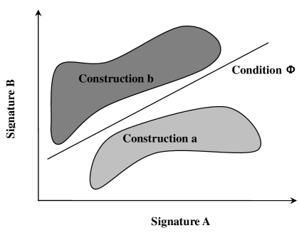
Figure 1: Cartoon to illustrate the method used to distinguish constructions.

The counting signatures in Table 2 denote numbers of events in excess of the Standard Model (SM). A description of some of the SM backgrounds included is in the next section.

Simple Criterion for Distinguishing Constructions

Based on the above pattern table, our criterion for distinguishing any given pair of constructions (a “Yes” in the pattern table) is that their respective entries are very different in at least one column, such as an $OC$ for one construction while an $ONC$ or $N.O.$ for another construction. A $Both$ for one construction while an $OC$ or $ONC$ or $N.O.$ for another does not distinguish the constructions cleanly. If there is only a small region of overlap between the two constructions for all signatures, then the two constructions can be distinguished in the regions in which they don’t overlap. This would give a “Probably Yes (PY)” in the pattern table, otherwise it would give a “Probably No (PN)”. Similarly, an $ONC$ for one construction and an $N.O.$ for another also does not distinguish the two constructions cleanly, and would give a “PY” or “PN” depending on their overlap. Carrying out this procedure for all constructions and signatures gives the result in Table 1. It should be kept in mind though that the result shown in Table 1 is only for a simple set of signatures. Using more sophisticated signatures and analysis techniques could give better resulst. Also, there are typically other useful signatures present than what is listed in the Table. We have only shown the most useful ones. In section VII, we give a description of the useful signatures and explain why these particular signatures are useful in distinguishing the various constructions in terms of the spectrum, the soft terms and in turn from the underlying theoretical structure.

VI Procedural Details

In this section we enumerate the procedure to answer question (A) in the Introduction, namely, how to go from a string construction to the space of LHC signatures.

The first step concerns the spectrum of a given construction. Many of the string-motivated constructions considered give a semi-realistic spectrum which contains the MSSM, and perhaps also some exotics. However for simplicity, in this initial analysis we only consider the MSSM fields because mechanisms may exist which project the exotic fields out or make them heavy. As already explained, for the KKLT and Large Volume vacua, we just assume the existence of an MSSM matter embedding. The weakly and strongly coupled heterotic string constructions are naturally compatible with gauge coupling unification at $M_{unif}\sim 2\times 10^{16}$ GeV, but type II-A and type II-B constructions are not in general. One can however try to impose that as an additional constraint even for type II constructions since gauge unification provides a very important clue to beyond-the-Standard Model physics. Therefore, all constructions except the Large Volume compactifications (IIB-L) used in our analysis either naturally predict or consistently assume the existence of gauge coupling unification at $M_{unif}$. The IIB-L construction does not have the possibility of gauge coupling unification at $M_{unif}$ compatible with having a supersymmetry breaking scale of $\mathcal{O}$(TeV) Balasubramanian:2005zx . The string scale for the IIB-L constructions is taken to be of $\mathcal{O}(10^{10}-10^{11})$ GeV in order to have a supersymmetry breaking scale of $\mathcal{O}$(TeV), making it incompatible with standard gauge unification.

In order to connect to low energy four-dimensional physics, one has to write the effective four dimensional action at the String scale /11 dim Planck scale, which we will denote by $M_{s}$. $M_{s}$ will be equated to $M_{unif}$ for all constructions except for the Large Volume compactifications (IIB-L). The four-dimensional effective action for each of these constructions is determined by a set of microscopic “input” parameters of the underlying theory. Soft supersymmetry breaking parameters for the MSSM fields are calculated at $M_{s}$ as functions of these underlying input parameters. A description of these input parameters can be found in section IV for the KKLT and Large Volume vacua, and in the Appendix for all the string-motivated constructions. The input parameters are taken to vary within appropriate ranges, as determined by theoretical and phenomenological considerations. In a more realistic construction, some of these parameters may actually be fixed by the theory. Our approach therefore is broad in the sense that we include a wide range of possibilities without restricting too much to a particular one.

Each of the “models” for a particular construction is thus defined by a list of input parameters which in turn translate to a parameter space of soft parameters at the unification scale. In other words, the boundary conditions for the soft parameters are determined by the underlying microscopic constructions. As emphasized earlier, this is very different from an ad hoc choice of boundary conditions for the soft parameters, as in many models like mSUGRA or minimal gauge mediation.

Once the soft parameters are determined from the underlying microscopic parameters, then the procedure to connect these soft parameters to low-scale physics is standard, namely, the soft parameters are evolved through the Renormalization Group (RG) evolution programs (SuSPECT Djouadi:2002ze and SOFTSUSY Allanach:2001kg ) to the electroweak scale, and the spectrum of particles produced is calculated. For concreteness and simplicity, we assume that no intermediate scale physics exists between the electroweak scale and the unification scale, though we wish to study constructions with intermediate scale physics and other subtleties in the future.

Of all the models thus generated, only some will be consistent with low energy experimental and observational constraints. Some of the most important low energy constraints are :

• Electroweak symmetry breaking (EWSB).

• Experimental bounds for superpartner masses.

• Experimental bound for the Higgs mass.

• Constraints from flavor and CP physics.

• Upper bound on the relic density from WMAP Bennett:2003bz .

In this analysis, we use $\tan\beta$ as an input parameter and the RGE software package determines $\mu$ and $B\mu$ by requiring consistent EWSB. This is because none of the constructions studied are sufficiently well developed so as to predict these quantities a priori. In the future, we hope to consider constructions which predict $\mu$, $B\mu$ and the Yukawa couplings allowing us to deduce $\tan\beta$ at the electroweak scale and explain EWSB. The models we consider are consistent with constraints on particle spectra, $b\rightarrow s\gamma$ Abe:2001hk , $(g_{\mu}-2)$ Bennett:2002jb and the upper bound on relic density. One should not impose the lower bound on relic density since non-thermal mechanisms can turn a small relic density into a larger one. Also, the usually talked about lower bound on the LSP mass ($\sim 50$ GeV) is only present for models with gaugino mass unification. There is no general lower bound on the LSP mass, especially if one also relaxes the constraint of a thermal relic density. In our analysis, we have not imposed any lower bound on the LSP mass. In our study at present, we have generated $\sim 50$ models for most constructions ($\sim 100$ models for the PH-A construction). This might seem too small at first. However from our analysis it seems that the results we obtain are robust and do not change when more points are added. For a purely statistical analysis this could be a weak point, but because in each case we know the connection between the theory and signatures and understand why the points populate the region they do, we expect stable results. We simulated many more models for two particular constructions and found that the qualitative results do not change, confirming our expectations. This will be explained in section IX.

Once one obtains the spectrum of superpartners at the low scale, one calculates matrix elements for relevant physics processes at parton level which are then evolved to “long-distance” physics, accounting for the conversion of quarks and gluons into jets of hadrons, decays of tau leptons,etc. We carry out this procedure using PYTHIA 6.324 Sjostrand:2003wg . The resulting hadrons, leptons and photons have to be then run through a detector simulation program which simulates a real detector. This was done by piping the PYTHIA output to a modified CDF fast detector simulation program PGS pgs . The modified version was developed by John Conway, Stephen Mrenna and others and approximates an ATLAS or CMS-like detector. The output of the PGS program is in a format which is also used in the LHC Olympics LHCO . It consists of a list of objects in each event labelled by their identity and their four-vector. Lepton objects are also labelled by their charges and b-jets are tagged. With this help of these, one can construct a wide variety of signatures.

The precise definitions of jets and isolated leptons, criteria for hadronically decaying taus, efficiencies for heavy flavor tagging as well as trigger-level cuts imposed on objects are the same as used for the “blackbox” data files in the LHC Olympics LHCO . In addition, we impose event selection cuts as the following:

• If the event has photons, electrons, muons or hadronic taus, we only select the particles which satisfy the following – Photon $P_{T}\;>10$ GeV; Electron, Muon $P_{T}\;>10$ GeV; (hadronic) Tau $P_{T}\;>100$ GeV.

• For any event with jets, we only select jets with $P_{T}\;>100$ GeV.

• Only those events are selected with $E\kern-6.00006pt\hbox{/}\kern 0.50003pt_{T}\;$ in the event $>100$ GeV.

These selection cuts are quite simple and standard. We have used a simple and relatively “broad-brush” set of cuts since for a preliminary analysis, we want to analyze many constructions simultaneously. As mentioned before, we have simulated 5 $fb^{-1}$ of data at the LHC for each model. A small luminosity was chosen for two reasons – first, in the interest of computing time and second, in order to argue that our proposed technique is powerful enough to distinguish between different constructions even with a limited amount of data. Of course, to go further than distinguishing classes of constructions broadly from relatively simple signatures, such as getting more insights about particular models within a given construction, one would in general require more data and could sharpen the approach by imposing more exclusive cuts and signatures.

In order to be realistic, one has to take the effects of the standard model background into account. In our analysis, we have simulated the $t\bar{t}$ background and the diboson ($WW,ZZ$)+ jets background. We have not included the uniboson ($W,Z$) + jets background in the interest of time. However, from Baer:1995va we know that for a $E\kern-6.00006pt\hbox{/}\kern 0.50003pt_{T}$ threshold of 100 GeV, as has been used in our analysis, the $t\bar{t}$ background is either the largest background or comparable to the largest one ($W$ + jets typically). Therefore, we expect our analysis and results to be robust against addition of the $W$ + jets background. The criteria we employ for an observable signature is :

$$\frac{N_{signal}}{\sqrt{N_{bkgd}}}>4;\;\;\frac{N_{signal}}{N_{bkgd}}>0.1;\;\;N_{signal}>5.$$ (1)

These conditions are quite standard. A signature is observable only when the most stringent of the three constraints is satisfied.

Although the steps used in our analysis are quite standard, there are at least two respects in which our analysis differs from that of previous ones in the literature. First, our work shows for the first time that with a few reasonable assumptions, one can study string theory constructions to the extent that reliable predictions for experimental observables can be made, and more importantly, different string constructions give rise to overlapping but distinguishable footprints in signature space. Moreover, it is possible to understand why particular combinations of signatures are helpful in distinguishing different constructions, from the underlying theoretical structure of the constructions. Therefore, even though we have done a simplified (but reasonably realistic) analysis in terms of trigger and selection level cuts, detection efficiencies of particles, detector simulation and calculation of backgrounds, we expect that doing a more sophisticated analysis will only change some of the details but not the qualitative results. In particular, it will not affect the properties that predictions for experimental observables can be made for many classes of realistic string constructions, and that patterns of signatures are sensitive to the structure of the underlying string constructions, making it possible to distinguish among various classes of string constructions.

VII Distinguishibility of Constructions

VII.1 General Remarks

For convenience, we present the signature pattern table again. As was also mentioned in section V, each signature has been broadly divided into two main classes for simplicity. The value of the observable dividing the two classes is chosen so as to yield the best results. A description of the most useful signatures is given below:

Signature		A	B	C	D	E	F	G
Condition		$>1200$	$>25$	$>1.6$	$>0.54$	$>0.05$	$>160$GeV	$>0.58$
HM-A		OC	OC	OC	OC	OC	Both	OC
HM-B		Both	Both	Both	Both	Both	Both	Both
HM-C		Both	Both	OC	Both	Both	Both	Both
PH-A		ONC	N.O.	OC	Both	ONC	ONC	Both
PH-B		N.O.	N.O.	N.O.	N.O.	N.O.	Both	N.O.
II-A		ONC	N.O.	ONC	OC	ONC	ONC	ONC
IIB-K		ONC	ONC	OC	ONC	Both	OC	ONC
IIB-L		ONC	N.O.	OC	Both	ONC	ONC	Both

Table 3: The String Pattern Table
An “$OC$” for the $i^{th}$ row and $j^{th}$ column means that the signature is observable for many models of the $i^{th}$ construction. The value of the $j^{th}$ signature for the $i^{th}$ construction is (almost) always consistent with the condition in the second row and $j^{th}$ column of the Table. An “$ONC$” also means that the signature is observable for many models of $i^{th}$ construction. However, the value of the signature (almost) always does not consistent with the condition as specified in the second row and $j^{th}$ column of the Table. A “$Both$” means that some models of the $i^{th}$ construction have values of the $j^{th}$ signature which are consistent the condition in the second row and the $j^{th}$ column while other models of the $i^{th}$ construction have values of the $j^{th}$ signature which are not consistent with the condition. An “N.O.” for the $i^{th}$ row and $j^{th}$ column implies that the $j^{th}$ signature is not observable for the $i^{th}$ construction, i.e. the values of the observable for all (most) models of the construction are always below the observable limit as defined by (1), for the given luminosity (5 $fb^{-1}$). So, the construction is not observable in the $j^{th}$ signature channel with the given amount of “data”.

• A – Number of events with trileptons and $\geq 2$ jets. The value of the observable dividing the signature into two classes is 1200.

• B – Number of events with clean (not accompanied by jets) dileptons. The value of the observable dividing the signature into two classes is 25.

• C – $(Y/X)$ ; Y= Number of events with 2 leptons, 0 b jets and $\geq 2$ jets, X= Number of events with 0 leptons, 1 or 2 b jets and $\geq 6$ jets. The value of the observable dividing the signature into two classes is 1.6.

• D – $(Y/X)$; Y= Number of events with 2 leptons, 1 or 2 b jets and $\geq 2$ jets, X= Number of events with 2 leptons, 0 b jets and $\geq 2$ jets. The value of the observable dividing the signature into two classes is 0.54.

• E – The charge asymmetry in events with one electron or muon and $\geq$ 2 jets ($A_{c}^{(1)}=\frac{N(l^{+})-N(l^{-})}{N(l^{+})+N(l^{-})}$). The value of the observable dividing the signature into two classes is 0.065.

• F – The peak of the missing energy distribution. The value of the observable dividing the signature into two classes is 160 GeV.

• G – $Y/X$; Y = Number of events with same sign different flavor (SSDF) dileptons and $\geq 2$ jets, X = Number of events with 1 tau and $\geq$ 2 jets. The value of the observable dividing the signature into two classes is 0.5.

The signatures A-F turn out to be the most economic and useful in distinguishing all constructions considered. We have also listed signature G as an example to show that it is possible to construct other signatures which can distinguish among some of the constructions. We understand that some of these signatures are not very realistic. For example, the signature which counts the number of events with 0 leptons, 1 or 2 b jets and $\geq$ 6 jets is not very realistic initially because of difficulties associated with calibrating the fake missing $E\kern-6.00006pt\hbox{/}\kern 0.50003pt_{T}$ from jet mismeasurement in events with six or more jets. However, we have used this signature in our analysis at this stage because it helps in explaining our results and the approach in an economic way. Also, the fact that there are other useful signatures which distinguish these constructions gives us additional confidence about the robustness of our approach. These signatures were hand-picked by experience and by trial-and-error. Once the set of useful signatures was collected, the next task was to understand why the above set of signatures were useful in distinguishing the constructions based on their spectrum, soft parameters and their underlying theoretical setup. This is the subject of sections VII.3, VII.4 and VII.5 respectively. We hope that carrying out the same exercise for other constructions can help build intuition about the kind of signatures which any given theory can produce. This can eventually help in building a dictionary between structure of underlying theoretical constructions and their collider signatures.

The above list of signatures consists of counting signatures and distribution signatures at the LHC. The counting signatures denote number of events in excess of the Standard Model. Naively, one would think that the number of signatures is very large if one includes lepton charge and flavor information, and $b$ jet tagging. However, it turns out that not all signatures are independent. In fact, they can be highly correlated with each other, drastically decreasing the effective dimensionality of signature space. Thus, in order to effectively distinguish signatures, one needs to use signatures sufficiently orthogonal to each other. This has been emphasized recently in Arkani-Hamed:2005px . We will see that having an underlying theoretical construction allows us to actually find those useful signatures. Even though we have only listed a few useful signatures in Table 2, there are typically more than one (sometimes many) signatures which distinguish any two particular constructions. This is made possible by a knowledge of the structure of the underlying theoretical constructions.

VII.2 Why is it possible to distinguish different Constructions?

In view of the above comments, one would like to understand why it is possible to distinguish different constructions in general and why the signatures described in the previous section are useful in distinguishing the various constructions in particular.

To understand the origin of distinguishibility of constructions, one should first understand why each construction gives rise to a specific pattern of soft supersymmetry breaking parameters and in turn to a specific pattern of signatures. This is mainly due to correlations in parameter space as well as in signature space. Let’s explain this in detail. A construction is characterized by its spectrum and couplings in general. These depend on the underlying structure of the theoretical construction, such as the form of the four-dimensional effective action, the mechanism to generate the hierarchy, the details of moduli stabilization and supersymmetry breaking, mediation of supersymmetry breaking etc. At the end of the day, the theoretical construction is defined by a small set of microscopic input parameters in terms of which all the soft supersymmetry breaking parameters are computed. Since all soft parameters are calculated from the same set of underlying input parameters, this gives rise to correlations in the space of soft parameters for any given construction. These correlations carry through all the way to low energy experimental observables, as will be explicitly seen later. The fact that there exist correlations between different sets of parameters which have their origin in the underlying theoretical structure allows us to gain insights about the underlying theory, and is much more powerful than completely phenomenological parameterizations such as mSUGRA, minimal gauge mediation, etc.

Since any two different theoretical constructions will differ in their underlying structure in some way by definition, the correlations obtained in their parameter and signature spaces will also be different in general. All these will in general have different effects on issues which influence low energy phenomenology in an important manner, such as the scale of supersymmetry breaking, unification of gauge couplings (or not), flavor physics, origins of CP violation, etc. These factors combined with experimental constraints allow different string constructions to be distinguished from each other in general.

We now wish to understand why the particular signatures described in section VII.1 are useful in distinguishing the studied constructions. In order to successfully do so, one has to understand the relevant features of the various constructions and their implications to hadron collider phenomenology, and devise signatures which are sensitive to those features.

In the following subsections, we explain how to distinguish the above constructions. In principle, one could directly try to connect patterns of signatures to underlying string constructions. However, in practice it is helpful to divide the whole process of connecting patterns of signatures to theoretical constructions in a few parts – first, the results of the pattern table for each construction are explained based on the spectrum of particles at the low scale; second, important features of the spectrum of superpartners at the low scale for the different constructions (which give rise to their characteristic signature patterns) are explained in terms of the soft supersymmetry breaking parameters at the high scale; and third, the structure of the soft parameters is explained in terms of the underlying theoretical structure of the constructions.

For readers not interested in the details in the next subsection, the main points to take away are that any given theoretical construction only gives rise to a specific pattern of observable signatures, and that one can understand and trust the regions of signature space that are populated by a given theoretical construction and that such regions are quite different for different constructions, illustrating in detail that LHC signatures can distinguish different theoretical constructions.

VII.3 Explanation of Signatures from the Spectrum

In this subsection, we take the spectrum pattern for different constructions as given and explain patterns of signatures based on them. Then it is possible to treat all the constructions equally as far as the explanation of the pattern of signatures from the spectrum is concerned. The characteristic features of the spectrum for the constructions considered are as follows:

• HM-A - Universal soft terms. Bino LSP (“coannihilation region”). Moderate gluinos (550-650 GeV), slightly lighter scalars.

• HM-B – Universal soft terms. Has two (disconnected) regions. Region I similar to HM-A. Region II either “focus point region” or “funnel region” Scalars much heavier ($>800$ GeV) than gauginos in region II.

• HM-C – Non-universal soft terms. Occupies a big region in signature space encompassing the two regions mentioned for the HM-B construction. Heavy scalars. Can have bino, wino or higgsino LSP. Spectrum and signature pattern quite complicated.

• PH-A — Non-universal soft terms. Bino, higgsino or mixed bino-higgsino LSP. Bino LSP has light gluino ($<600$ GeV). Higgsino or mixed bino-higgsino LSP have gluinos ranging from moderately heavy to heavy ($600-1200$ GeV). Heavy scalar masses ($\geq 2$ TeV).

• PH-B – Non-universal soft terms. Wino and bino LSP. Light gluinos (200-550 GeV) always have wino LSPs while heavier gluinos can have bino or wino LSPs. Comparatively heavy LSP (can be upto 1 TeV), heavy scalar masses ($\geq 1$ TeV) except stau which is relatively light ($\geq 500$ GeV).

• II-A – Non-universal soft terms. Can have bino, wino, higgsino or mixed bino-higgsino LSP. Light or moderately heavy gluino ($300-600$ GeV), scalar masses heavier than gluinos but not very heavy ($<1$ TeV). Stops can be as light as 500 GeV. Spectrum and signature pattern quite complicated.

• IIB-K – Non-universal soft terms. Heavy spectrum ($\geq$ 1 TeV) in general, but possible to have light spectrum ($\leq$ 1 TeV). Bino LSP. Gluinos are greater than about $450$ GeV while the lightest squarks ($\tilde{t}_{1}$) are greater than about $200$ GeV. For some models, $\tilde{\tau}_{1}$ can be light as well.

• IIB-L – Non-universal soft terms. Mixed bino-higgsino LSP. The gluinos have a lower bound of about $350$ GeV, while the lightest squark ($\tilde{t}_{1}$) has a lower bound of about 700 GeV.

As mentioned in the list of characteristic features of the spectrum above, the HM-B and HM-C constructions roughly occupy two regions in signature space, as can be seen from Figure 2. One of these regions overlaps with the HM-A construction. This is because the HM-B and HM-C constructions contain the HM-A construction as a subset (see the Appendix for details). Since the three constructions have the same theoretical structure in a region of their high scale parameter space, the models of the three constructions in that particular region cannot be distinguished from each other from their signature pattern as their signatures will always overlap. However, since the HM-B and HM-C constructions have a bigger parameter space, they also occupy a bigger region of signature space compared to the HM-A construction. Thus, it is possible to distinguish the HM-A, HM-B and HM-C constructions in regions in which they don’t overlap, i.e. in regions in which their underlying theoretical structure is different. This is the origin of “Probably Yes (PY)” in Table 1.

Figures 2 and 3 shows two (very) inclusive signature plots. One can try to explain the differences in these signatures among the HM-A construction and the overlapping HM-B and HM-C constructions on the one hand and the PH-A, PH-B, II-A, IIB-K and IIB-L constructions on the other, from their spectra.

The HM-A construction and the overlapping HM-B, HM-C constructions have a comparatively light spectrum at the low scale. These give rise to a subset of the well known mSUGRA boundary conditions, so after imposing constraints from low energy physics as in section VI, one finds that the allowed spectrum consists of light and moderately heavy gluinos, slightly lighter squarks and light sleptons. Thus, $\tilde{g}\tilde{q}$ production and $\tilde{q}\tilde{q}$ pair production are dominant with direct $\tilde{N_{2}}\,\tilde{C_{1}}$ production also quite important.

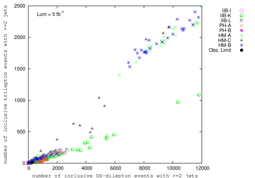
Figure 2: Plot of number of events with opposite-sign dileptons and $\geq$ 2 jets and number of events with three leptons and $\geq$ 2 jets. The black dot represents the lower limit of observability of the two signatures, according to conditions in equation (1). Note that the HM-A and overlaping HM-B and HM-C construction can be distinguished easily from the PH-A, PH-B, II-A, IIB-K and IIB-L constructions, as they occupy very different regions. The plots are best seen in color.

Both squarks and gluinos ultimately decay to $\tilde{N_{2}}$ and $\tilde{C_{1}}$ and since most sleptons (including selectrons, smuons) are accessible, both $\tilde{N_{2}}$ and $\tilde{C_{1}}$ decay to leptons and the LSP via sleptons. Since the mass difference between $\tilde{N_{2}}$, $\tilde{C_{1}}$ and LSP ($\tilde{N_{1}}$) is big (because of universal boundary conditions, $\Delta M_{\tilde{N_{2}}-\tilde{N_{1}}},\Delta M_{\tilde{C_{1}}-\tilde{N_{1}}}\sim M_{\tilde{N_{1}}}$), most of the leptons produced pass the cuts. The $\tilde{N_{2}}$ and $\tilde{C_{1}}$ by themselves are also comparatively light ($<200$ GeV). On the other hand, the PH-A, PH-B, II-A and IIB-L constructions are required to have heavy scalars and gluinos varying in mass from light to heavy. So, the $\tilde{N_{2}}$ and $\tilde{C_{1}}$ produced from gluinos decay to the LSP mostly through a virtual $Z$ and $W$ respectively, which makes their branching ratio to leptons much smaller. Because of non-universal soft terms, $\Delta M_{\tilde{N_{2}}-\tilde{N_{1}}}$ and $\Delta M_{\tilde{C_{1}}-\tilde{N_{1}}}$ can be bigger or smaller than in the universal case. In the PH-A, PH-B, II-A and IIB-L constructions, they are required to be comparatively smaller, leading to leptons which are comparatively softer on average, many of which do not pass the cuts.

For clean dilepton events, direct production of $\tilde{N_{2}}$ and $\tilde{C_{1}}$ is required. The HM-A construction and overlapping HM-B and HM-C constructions have comparatively lighter $\tilde{N_{2}}$ and $\tilde{C_{1}}$, so $\tilde{N_{2}}$ and $\tilde{C_{1}}$ are directly produced. On the other hand, most models of the PH-B and II-A constructions have heavier $\tilde{N_{2}}$ and $\tilde{C_{1}}$ compared to the HM-A construction, making it harder to produce them directly. The PH-A and IIB-L constructions have some models with light $\tilde{N_{2}}$ and $\tilde{C_{1}}$, but the other factors (decay via virtual W and Z, and smaller mass separation between $\tilde{N_{2}}$, $\tilde{C_{1}}$ and LSP) turn out to be more important, leading to no observable clean dilepton events. Therefore, the result is that none of the models of the PH-A, PH-B, II-A and IIB-L constructions have observable clean dilepton events. Thus, it is possible to distinguish the HM-A construction and overlapping HM-B and HM-C constructions from the PH-A, PH-B, II-A and IIB-L constructions by signatures A and B in Table 3 (shown in Figures 2 and 3).

The case with the IIB-K construction is slightly different. These constructions have many models with a heavy spectrum which implies that those models do not have observable events with the given luminosity of 5 $fb^{-1}$. However, these constructions can also have light gluinos and squarks with staus also being light in some cases. So $\tilde{g}\tilde{q}$ production is typically dominant for these models. The gluinos and squarks decay to $\tilde{N_{2}}$ and $\tilde{C_{1}}$ as for other constructions. Since for many IIB-K models, the lightest stau is heavier than $\tilde{N_{2}}$ and $\tilde{C_{1}}$ (even though it is relatively lighter than in the PH-A, PH-B, II-A and IIB-L constructions), the $\tilde{N_{2}}$ and $\tilde{C_{1}}$ decay to the LSP through a virtual $Z$ and $W$ respectively, making the branching fraction to leptons much smaller than for the HM-A and overlapping HM-B and HM-C constructions. In addition, the mass differences $\Delta M_{\tilde{N_{2}}-\tilde{N_{1}}}$ and $\Delta M_{\tilde{C_{1}}-\tilde{N_{1}}}$ are required to be smaller for the IIB-K construction in general compared to that for the HM-A and overlapping HM-B and HM-C constructions, making it harder for the leptons to pass the cuts. Some IIB-K models have comparable mass differences $\Delta M_{\tilde{N_{2}}-\tilde{N_{1}}}$ and $\Delta M_{\tilde{C_{1}}-\tilde{N_{1}}}$ as the HM-A construction, but they have much heavier gluinos compared to those for the HM-A construction, making their overall cross-section much smaller. Therefore, the IIB-K construction has fewer events for leptons in general (in particular for trileptons) compared to that for the HM-A and overlapping HM-B and HM-C constructions, as seen from Figure 2.

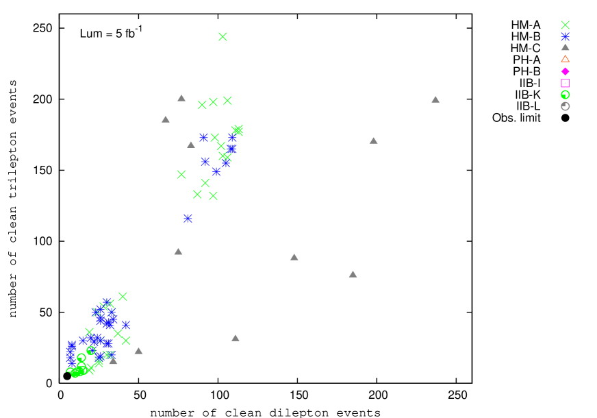
Figure 3: Plot of number of events with clean dileptons and number of events with clean trileptons. “clean” means not accompanied by jets. The black dot represents the lower limit of observability of the two signatures, according to conditions in equation (1). The models below the observable limit have not been shown. Note that the HM-A and overlapping HM-B and HM-C constructions can be distinguished from the PH-A, PH-B, II-A and IIB-L constructions, since the latter are not observable with the given luminosity. The plots are best seen in color.

Region II of the HM-B construction and the non-overlapping region of the HM-C construction (with HM-A) cannot be cleanly distinguished from the PH-A, PH-B, II-A, IIB-K and IIB-L constructions from the above signatures. Region II of the HM-B construction (the “focus point” or “funnel region” of mSUGRA) however, can be distinguished from these constructions with the help of other signatures. The entries for the HM-B construction in Table 3 correspond to the overall HM-B region, which explains the “Both” in all columns for the HM-B construction. Since one can distinguish region II of HM-B with other constructions by using other signatures as explained in the footnote, inspite of the “Both” entry in Table 3 one has a “Yes” for the HM-B row in the appropriate columns in Table 1. The non-overlapping region of the HM-C construction is a very big region in signature space because of its big parameter space (explained in the Appendix), making it relatively harder to distinguish it from some of the other constructions. Since we have not found signatures cleanly distinguishing the whole msoft-II region from some of the other constructions, we have put a “Probably Yes” for the HM-C row in the appropriate columns in Table 1.

Now we explain the distinguishibility of the PH-A, PH-B, II-A, IIB-K and IIB-L constructions. Figure 4 shows that the PH-B and II-A constructions can be distinguished from the PH-A, IIB-K and IIB-L constructions (signature $C$ in Table 3). Figure 5 shows that the PH-B and II-A constructions can be distinguished from each other and that the PH-A and IIB-L constructions can be partially distinguished from each other (signature $D$ in Table 3). To understand why it is possible to do so, we look at these constructions in detail.

Let’s start with the IIB-K construction. As explained earlier, the IIB-K construction typically gives a heavy spectrum, although it is possible to have a light spectrum with light gluinos and squarks (stops) with the stau also being light in some cases. So, $\tilde{g}\tilde{q}$ production is typically dominant. First and second generation squarks are copiously produced. The first and second generation squarks decay to non b-jets and the gluino also decays more to non b jets than to b jets because the IIB-K construction always has a bino LSP. Therefore, as seen from Figure 5, the IIB-K construction has more events with 2 leptons, 0 b jets and $\geq$ 2 jets compared to those with 2 leptons, 1 or 2 b jets and $\geq$ 2 jets. Also, since the mass difference between $\tilde{N_{2}},\tilde{C_{1}}$ and $\tilde{N_{1}}$ is only big enough for leptons to pass the cuts but not for jets to pass the cuts, the number of events with 0 leptons, 1 or 2 b jets and $\geq$ 6 jets is smaller than those with 2 leptons, 0 b jets and $\geq$ 2 jets, as seen from Figure 4.

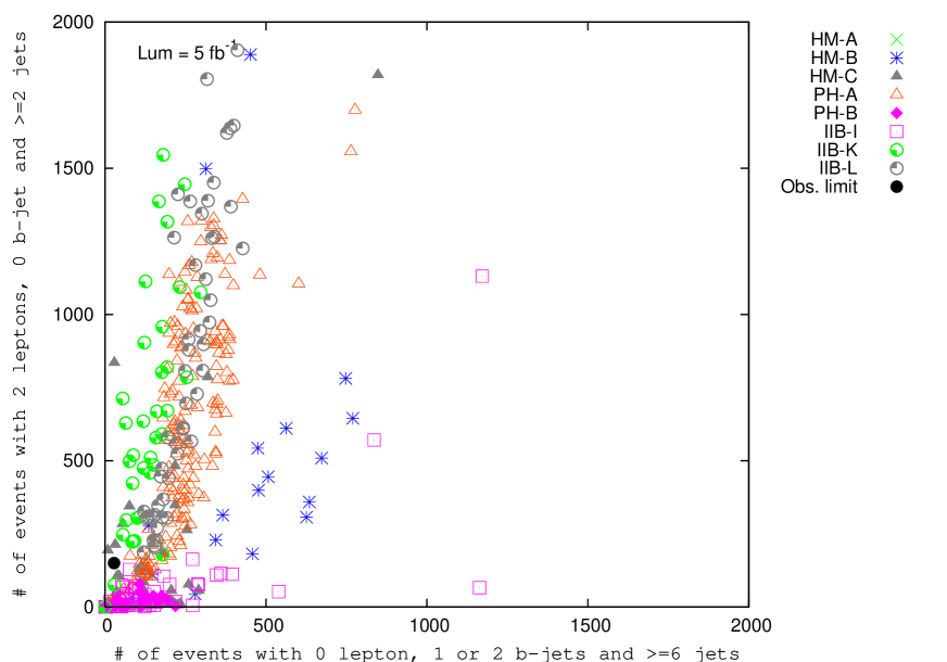
Figure 4: Plot of number of events with 0 leptons, 1 or 2 b jets and $\geq$ 6 jets and number of events with 2 leptons, 0 b jets and $\geq$ 2 jets. The black dot represents the lower limit of observability of the two signatures, according to conditions in equation (1). The models below the observable limit have also been shown to emphasize that the II-A construction has very different number of events for these signatures compared to other constructions even without imposing the observability constraint. Note that the PH-B and II-A constructions can be distinguished from the PH-A, IIB-K and IIB-L constructions because they have very different slopes. The plots are best seen in color.

The PH-B construction has scalars which are quite heavy ($>1$ TeV). So, gluino pair production is dominant. The branching ratio of gluinos to $\tilde{C_{1}}$ + jets is typically the largest for $\tan\beta\geq 20$, if it is kinematically allowed Bartl:1994bu , followed by $\tilde{N_{i}}$ + jets, $i=1,2,3$, which are smaller. This is generally true for this construction.

When the gluino is light ($\leq 550$ GeV), the PH-B construction has wino LSP. Since $\mu$ is large ($>1.3$ TeV), $m_{\tilde{C_{1}}}\sim m_{\tilde{N_{1}}}$. Since $\tilde{C_{1}}$ and $\tilde{N_{1}}$ are wino and $\tilde{N_{2}}$ is bino, the gluino decays mostly to non b jets. Also, the leptons and jets coming from the decay of $\tilde{C_{1}}$ to $\tilde{N_{1}}$ are very soft and do not pass the cuts. When the gluino directly decays to $\tilde{N_{1}}$, there are no leptons and only two jets. When the gluino is heavier ($>550$ GeV), the PH-B construction can have wino as well as bino LSPs. Because of a heavier gluino, the overall cross-section goes down. For the wino LSP case, the same argument as above applies in addition to the small cross-section implying even fewer lepton events. For the bino LSP case, the gluino again decays mostly to non b jets as $\tilde{C_{1}}$ and $\tilde{N_{2}}$ are wino and $\tilde{N_{1}}$ is bino. Also, $m_{\tilde{C_{1}}}\sim m_{\tilde{N_{2}}}$ but at the same time $\Delta M_{\tilde{N_{2}}-\tilde{N_{1}}}$ and $\Delta M_{\tilde{C_{1}}-\tilde{N_{1}}}$ are quite small ($\leq 20$ GeV), leading to soft leptons and jets many of which don’t pass the cuts. So the result is that PH-B models have very few events with leptons and/or b jets. Therefore, as seen from Figures 4 and 5, the PH-B construction does not give rise to observable events for signatures $D$ and $E$ in Table 3.

Figure 5: Plot of number of events with 2 leptons, 0 b jets and $\geq$ 2 jets and number of events with 2 leptons, 1 or 2 b jets and $\geq$ 2 jets. The black dot represents the lower limit of observability of the two signatures, according to conditions in equation (1). The models below the observable limit have not been shown. Note that the PH-B and II-A constructions can be distinguished from each other since the former is not observable while the latter is observable. One can also partially distinguish the PH-A and IIB-L constructions. The plots are best seen in color.

The PH-A construction is required to have bino, higgsino or mixed bino-higgsino LSP with very heavy scalar masses ($\geq 2$ TeV). Light gluinos ($\leq 600$ GeV) have bino LSP, while higgsino or mixed bino-higgsino LSPs have heavier gluinos ($600-1200$ GeV). $\tilde{N_{2}}$ and $\tilde{C_{1}}$ are also quite light ($<250$ GeV).

For the bino LSP case, gluinos typically decay to $\tilde{N_{1}}$, $\tilde{N_{2}}$ and $\tilde{C_{1}}$ and non b jets most of the time compared to b jets, as $\tilde{N_{1}}$ is bino and $\tilde{N_{2}}$ and $\tilde{C_{1}}$ are wino. The decays of $\tilde{N_{2}}$ and $\tilde{C_{1}}$ can give rise to leptons passing the cuts. In addition, direct production of $\tilde{N_{2}}$ and $\tilde{C_{1}}$ is also important as they are light. They can also give rise to 2 leptons, 0 b jets and $\geq 2$ jets. Therefore, in this case, one has more events with (two) leptons and non b jets compared to those with (two) leptons and b jets. This can be seen clearly from Figure 5. The decays of $\tilde{N_{2}}$ and $\tilde{C_{1}}$ also give jets (as they decay through virtual Z and W). Since the gluino is light, the cross-section is quite big implying that there are also a fair number of events with 0 leptons, 1 or 2 b jets and $\geq 6$ jets. However, the number of events with 2 leptons, 0 b jets and $\geq 2$ jets is more than with 0 leptons, 1 or 2 b jets and $\geq 6$ jets due to the dominant branching ratio of gluinos to non b jets. This can be seen from Figure 4.

For the higgsino LSP case, the gluino is comparatively heavier ($600-1200$ GeV), leading to a significant decrease in cross-section. Now $\tilde{N_{1}}$, $\tilde{N_{2}}$ and $\tilde{C_{1}}$ are mostly higgsino, leading to a lot of production of b jets as the relevant coupling is proportional to the mass of the associated quark. The fact that $\tilde{N_{1}}$, $\tilde{N_{2}}$ and $\tilde{C_{1}}$ are mostly higgsino also makes their masses quite close to each other, implying that leptons and jets produced from the decays of $\tilde{N_{2}}$ and $\tilde{C_{1}}$ to $\tilde{N_{1}}$ are very soft and do not pass the cuts. Thus, these models have very few events with leptons. Since the jets coming from the decays of $\tilde{N_{2}}$ and $\tilde{C_{1}}$ to $\tilde{N_{1}}$ are also very soft, the PH-A higgsino LSP models also have very few events with 0 leptons, 1 or 2 b jets and $\geq 6$ jets. Therefore, these do not give rise to observable events for the signatures in Figures 4 and 5.

For the mixed bino-higgsino LSP case, the gluino is again quite heavy ($600-1200$ GeV), making the cross section much smaller compared to the bino LSP case. Since $\tilde{N_{1}}$, $\tilde{N_{2}}$ and $\tilde{C_{1}}$ have a significant higgsino fraction, the gluinos again decay more to b jets compared to non b jets. The mass separation between $\{\tilde{N_{2}},\tilde{N_{3}},\tilde{C_{1}}\}$ and $\tilde{N_{1}}$ is such that the decays of $\tilde{N_{2}}$ and $\tilde{C_{1}}$ to $\tilde{N_{1}}$ produce leptons which typically pass the cuts and jets which only sometimes pass the cuts. Therefore, these PH-A models have few events with 2 leptons, 0 b jets and $\geq 2$ jets. They give rise to events with 2 leptons, 1 or 2 b jets and $\geq 2$ jets but since the overall cross-section is much smaller than for the bino LSP case, the number of events for the above signature for these PH-A models is just a little above the observable limit, as can be seen from Figure 5. This is the origin of the “Both” entry for signature $D$ in the row for the PH-A construction. Because of the small overall cross-section as well as the fact that jets produced from the decays of $\tilde{N_{2}}$ and $\tilde{C_{1}}$ only sometimes pass the cuts, the number of events for 0 leptons, 1 or 2 b jets and $\geq 6$ jets is also small for these PH-A models, as seen from Figure 4.

The IIB-L construction always has a mixed bino-higgsino LSP, for both light and heavy gluino models. The light gluino IIB-L models have a large overall cross-section. The gluinos decay both to non b jets and b jets owing to the mixed bino-higgsino nature of the LSP. Also, the mass separation between $\tilde{N_{2}}$, $\tilde{C_{1}}$ and $\tilde{N_{1}}$ is not large which means that the leptons produced from the decays of $\tilde{N_{2}}$ and $\tilde{C_{1}}$ pass the cuts but the jets produced seldom pass the cuts. So, the IIB-L construction has many events with 2 leptons, 0 b jets and $\geq$ 2 jets as well as with 2 leptons 1, or 2 b jets and $\geq$ 2 jets but not as many with 0 leptons, 1 or 2 b jets and $\geq$ 6 jets, as seen from Figures 4 and 5.

From Figure 5, one sees that the IIB-L construction can be distinguished partially from the PH-A construction, leading to a “Probably Yes (PY)” in the pattern table. One can understand it as follows - as mentioned above, the IIB-L construction always has a mixed bino-higgsino LSP while the PH-A construction has a mixed bino higgsino LSP only when the gluino is heavy (i.e. for a heavy spectrum). For light gluino models, as mentioned before, the PH-A construction has a bino LSP. Therefore, for light gluino models, the ratio of number of events with 2 leptons, 1 or 2 b jets and $\geq$ 2 jets and number of events with 2 leptons 0 b jets and $\geq$ 2 jets is much more for the IIB-L construction compared to the PH-A construction. These are the models which differentiate the IIB-L and PH-A constructions in Figure 5. It turns out that mixed bino-higgsino LSP models with heavy gluinos in both constructions have very similar spectra, leading to very similar signatures in all studied channels. Therefore, the IIB-L construction and the PH-A construction are not distinguishable in this special region of spectrum and signature space with the present set of signatures. Using more sophisticated signatures may help distinguish these signatures more cleanly. As already mentioned before, the PH-A construction also has models with a pure higgsino LSP. Those models have very heavy gluinos however, leading to no observable events in Figures 4 and 5.

Moving on to the II-A construction, we note that it can have a bino, wino, higgsino or mixed bino-higgsino LSP with light to moderately heavy gluino ($300-600$ GeV) and moderately heavier scalars (stops can be specially light). The spectrum and signature pattern are quite complicated. Let’s analyze all possible cases.

In this construction, the branching ratio of gluinos to $\tilde{C_{1}}$ + jets is the largest as mentioned before, since $\tan\beta\geq 20$. For the wino LSP case, since $M_{\tilde{C_{1}}}\sim M_{\tilde{N_{1}}}$ the leptons and jets from the decays of $\tilde{C_{1}}$ to $\tilde{N_{1}}$ are very soft and do not pass the cuts. The decay of the gluino to $\tilde{C_{1}}$ is accompanied by non b jets since $\tilde{N_{1}}$ and $\tilde{C_{1}}$ are wino and $\tilde{N_{2}}$ is bino. So, the II-A models with wino LSP do not give rise to observable events with leptons and/or b jets. This implies that the signatures in Figures 4 and 5 are not observable for these II-A models.

For the bino LSP case, $\tilde{N_{2}}$ and $\tilde{C_{1}}$ are quite heavy ($>350$ GeV), sometimes being even heavier than the gluino, in which case only the decay of gluino to $\tilde{N_{1}}$ is allowed leading to no leptons. Even when the decays of gluino to $\tilde{C_{1}}$ and $\tilde{N_{2}}$ are allowed, they are mostly accompanied by comparatively soft non b jets (due to kinematic reasons). Since these II-A models are required to have $\tilde{N_{2}}$ and $\tilde{C_{1}}$ much heavier than the PH-A bino LSP models, the direct production of $\tilde{N_{2}}$ and $\tilde{C_{1}}$ which could be a source of events with 2 leptons, 0 b jets and $\geq 2$ jets, is also relatively suppressed. Therefore these models do not give rise to observable events with 2 leptons 0 b jets and $\geq 2$ jets as well as with 2 leptons, 1 or 2 b jets and $\geq 2$ jets. However, there are some bino LSP II-A models which also have light squarks (stops mostly) and light gluinos in addition to having heavy $\tilde{N_{2}}$ and $\tilde{C_{1}}$ as above. For these bino LSP models, $\tilde{q}\tilde{q}$ pair production is quite important. These squarks mostly decay to a gluino and quarks, followed by the decay of the gluino to mostly the LSP and jets (both b and non b jets). Thus, these bino LSP II-A models have many events with 0 leptons, 1 or 2 b jets and $\geq 6$ jets but no observable events with 2 leptons, 1 or 2 b jets and $\geq 2$ jets.

For the higgsino LSP case, since $\tan\beta\geq 20$, the gluino mostly decays to $\tilde{C_{1}}$ + b jets as the associated coupling is proportional to the mass of the relevant quark. Also, in this case $\tilde{N_{1}}$, $\tilde{N_{2}}$ and $\tilde{C_{1}}$ are all higgsino like and very close to each other. So, leptons from the decays of $\tilde{N_{2}}$ and $\tilde{C_{1}}$ to $\tilde{N_{1}}$ are very soft and do not pass the cuts. Therefore II-A models with higgsino LSP do not give rise to observable events with leptons and/or non b jets. For some of these higgsino LSP II-A models, there are still a fair number of events with 0 leptons 1 or 2 b jets and $\geq 6$ jets. This is because even though $\tilde{q}\tilde{q}$ pair production is less important compared to those in bino LSP II-A models, the branching ratio of gluinos to b jets is much bigger (due to a higgsino LSP).

For the mixed bino-higgsino LSP case, the decay of gluino to $\tilde{C_{1}}$ + b jets is dominant since $\tilde{C_{1}}$ is mostly higgsino. The next important decays are to $\tilde{N_{1}}$, $\tilde{N_{2}}$ and $\tilde{N_{3}}$ + b jets followed by a small fraction to non b jets. The mass separation between $\{\tilde{N_{2}},\tilde{N_{3}},\tilde{C_{1}}\}$ and $\tilde{N_{1}}$ is such that leptons produced can easily pass the cuts, while the jets produced sometimes pass the cuts. Some of these mixed bino-higgsino LSP II-A models also have comparatively light squarks, implying that $\tilde{q}\tilde{q}$ and $\tilde{q}\tilde{g}$ production are also important. The squark decays to a quark and a gluino, followed by the usual decays of the gluino. For these models, $\tilde{N_{2}}$ and $\tilde{C_{1}}$ are also light, implying that in such cases direct production of $\tilde{N_{2}}$ and $\tilde{C_{1}}$ is also possible. The decays of $\tilde{N_{2}}$ and $\tilde{C_{1}}$ can give rise to events with 2 leptons, 0 b jets and $\geq 2$ jets.

Therefore, the conclusion is that for II-A models with mixed bino-higgsino LSP and light squarks, there are observable events with 2 leptons, 1 or 2 b jets and $\geq 2$ jets; with 0 leptons, 1 or 2 b jets and $\geq 6$ jets as well as with 2 leptons 0 b jets and $\geq 2$ jets. The number of events with 2 leptons, 1 or 2 b jets and $\geq 2$ jets is greater than those with 2 leptons, 0 b jets and $\geq 2$ jets because of the dominant branching fraction of gluinos to b jets. Therefore, signature $D$ (ratio of the above two type of events - Figure 5) can distinguish the II-A and PH-B constructions as the II-A construction has observable events while the PH-B construction does not give rise to observable events. The number of events for 0 leptons 1 or 2 b jets and $\geq 6$ jets will be larger than those with 2 leptons, 0 b jets and $\geq 2$ jets, again due to the dominant branching ratio of the gluino to b jets. So, signature $C$ (ratio of the above two type of events - Figure 4) can distinguish the PH-A,IIB-K and IIB-L constructions from the II-A and PH-B constructions. The above results can be seen from Figures 4 and 5, where the qualitative difference between the constructions is clear.

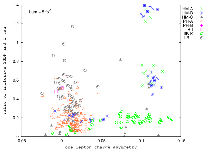
Figure 6: Plot of the charge asymmetry in events with a single electron or muon $\&\;\geq$ 2 jets $\&$ the ratio of number of events with same sign different flavor (SSDF) dileptons and $\geq$ 2 jets and number of events with 1 tau and $\geq$ 2 jets. The models which are below the observable limit as defined by (1) are not shown. Note that the IIB-K construction can be distinguished from the PH-A and IIB-L constructions, as the former occupies a mostly horizontal region while the latter occupy a mostly vertical region. The overlapping IIB-K and PH-A models can be distinguished from Figure 7. The plots are best seen in color.

The II-A models shown above the observable limit have mixed bino-higgsino LSP with lighter squarks than in other II-A cases.

We are now left with explaining the distinguishibility of the PH-A and IIB-L constructions on the one hand and the IIB-K construction on the other. Figures 6 and 7 show that the IIB-K construction can be distinguished from the PH-A and IIB-L constructions. The reason is as follows - As explained earlier, the IIB-K construction can have a light spectrum with light gluinos, light stop and sometimes a light stau. So, $\tilde{g}\tilde{q}$ production is typically dominant. Since up-type squarks are produced preferentially at the LHC (as it is a $pp$ collider), they decay preferentially to a positive chargino $\tilde{C}_{1}^{+}$, which in turn decays preferentially to a positively charged lepton $l^{+}$ (in its leptonic decays). Therefore, the asymmetry in number of events with a single electron or muon and $\geq$ 2 jets ($A_{c}^{(1)}$) is much greater than in the case of PH-A and IIB-L constructions where $\tilde{g}\tilde{g}$ pair production is dominant. There are a few IIB-K models which have a small $A_{c}^{(1)}$ and which overlap with some PH-A models (seen in Figure 6) even though $\tilde{g}\tilde{q}$ production is dominant. This is due to some special features of their spectrum, such as the lightest stop and/or the lightest stau being very light. These features either suppress the production of $\tilde{C}_{1}^{+}$ or suppress the decay of $\tilde{C}_{1}^{+}$ to electrons or muons. However, as seen from Figure 7, these overlapping IIB-K models can be distinguished from the PH-A and IIB-L constructions by the peak of the $E\kern-6.00006pt\hbox{/}\kern 0.50003pt_{T}$ distribution. This is related to the mass of the LSP. The IIB-K constructions (which are observable with 5 $fb^{-1}$) have a comparatively heavier LSP than the IIB-L constructions in general, making the peak of the $E\kern-6.00006pt\hbox{/}\kern 0.50003pt_{T}$ distribution larger than those for the IIB-L constructions. The PH-A models which overlap with the small $A_{c}^{(1)}$ IIB-K models have bino LSPs which are lighter than that of the IIB-K models. So, the PH-A models have a smaller $E\kern-6.00006pt\hbox{/}\kern 0.50003pt_{T}$ peak than the overlapping IIB-K models in Figure 6, as can be seen from Figure 7.

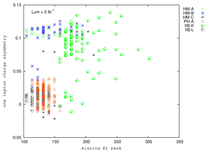
Figure 7: Plot of the peak of the $E\kern-4.80005pt\hbox{/}\kern 0.40002pt_{T}$ distribution and the charge asymmetry in events with a single electron or muon $\&\;\geq$ 2 jets. The models which are below the observable limit as defined by (1) are not shown. Note that this plot distinguishes the overlapping PH-A and IIB-K models in Figure 6. The plots are best seen in color.

We have thus explained the distinguishibility of all constructions based on the spectrum at the low scale. Typically, there are more than one (sometimes many) signatures which can distinguish any two given constructions. This redundancy gives us confidence that our analysis is robust and that the conclusions will not be affected with more sophisticated analysis. For simplicity, we have only explained one signature distinguishing a pair of constructions but all such signatures can be understood similarly.

VII.4 Explanation of Spectrum from the Soft Parameters

We now turn to understanding the origin of the spectrum of particles at the low scale (which are responsible for the signature pattern) for the constructions in terms of pattern of soft parameters. For illustrative purposes, we carry out this exercise for two constructions – the HM-A construction and the PH-B construction. If we take the soft parameters at the string (or unification) scale as given, then it does not matter that these are really only toy constructions. The kind of analysis carried out for these constructions below can also be carried out for more well motivated constructions such as the KKLT and Large Volume ones, as well. However, to go to the final step, i.e. from the soft parameters to the structure of the underlying theoretical construction, it makes sense to stick to the more well motivated constructions – the KKLT and Large Volume constructions, as we will in the following subsection.

Starting with the HM-A construction, one would like to understand its characteristic spectrum, viz. $m_{\tilde{g}}\sim m_{\tilde{q}}>m_{\tilde{l}}$. Why does the gluino mass lie in the range $550-650$ GeV? We note that the HM-A construction is a heterotic M theory construction compactified on a Calabi-Yau with only one Kähler modulus. This implies that the soft terms obtained at the unification scale are universal Choi:1997cm . Thus, the soft terms obtained at the unification scale are a special case of the well studied mSUGRA boundary condition. Now, phenomenological studies of the mSUGRA boundary condition have shown that in order to get a small relic density (satisfying the WMAP upper bound ), there are three allowed regions in the $m-M$ plane Ellis:2003cw . Here $m$ stands for the universal scalar mass parameter while $M$ stands for the universal gaugino mass parameter. These three regions are the following:

• The stau coannihilation region – In this region, the stau is almost degenerate with the LSP which is a bino. One gets an acceptable relic density because of coannihilation of the stau and the LSP to a tau. This requires $m<M$ with $m$ roughly between 100 and 150 GeV and $M$ roughly between 150 and 300 GeV (assuming $A_{0}$ = 0).

• The focus point region – This region requires a large scalar mass parameter ($m>M$) at the unification scale, and gives rise to a higgsino LSP with acceptable relic density.

• The funnel region – In this region, the LSP is annihilated by a $s$-channel pole, with $m_{LSP}\approx m_{A}/2$. This also requires $m>M$.

In the case of the HM-A construction, the soft mass parameters always have the hierarchy $M>m$ Choi:1997cm , which implies that only the stau coannihilation region is possible for the HM-A construction. Also, the allowed ranges for the $m$ and $M$ parameters roughly explains the mass scale of the gluino and squarks at the low scale from standard RG evolution. Therefore, one has to now understand the origin of the allowed values of the $m$ and $M$ parameters from the nature of the expressions for soft terms and the “theory” input parameters.

The expressions for the soft terms depend on three input parameters – the goldstino angle $\theta$, the gravitino mass $m_{3/2}$ and the parameter $\alpha(t+\bar{t})$ with $t$ as the Kähler modulus, in addition to $\tan{\beta}$. For futher details, the reader is referred to Choi:1997cm . The expressions for the soft parameters are given by :

$$M = \frac{\sqrt{3}Cm_{3/2}}{(s+\bar{s})+\alpha(t+\bar{t})}\{(s+\bar{s})\sin(\theta)e^{-i\gamma_{s}}+\frac{\alpha(t+\bar{t})}{\sqrt{3}}\cos(\theta)e^{-i\gamma_{t}}\}$$ (2)

$$m^{2} = V_{0}+m_{3/2}^{2}-\frac{3m_{3/2}^{2}C^{2}}{3(s+\bar{s})+\alpha(t+\bar{t})}\,\{\alpha(t+\bar{t})\,(2-\frac{\alpha(t+\bar{t})}{3(s+\bar{s})+\alpha(t+\bar{t})})\sin^{2}(\theta)+$$

$$(s+\bar{s})\,(2-\frac{3(s+\bar{s})}{3(s+\bar{s})+\alpha(t+\bar{t})})\cos^{2}(\theta)-\frac{2\sqrt{3}\alpha(t+\bar{t})(s+\bar{s})}{3(s+\bar{s})+\alpha(t+\bar{t})}\sin(\theta)\cos(\theta)\cos(\gamma_{s}-\gamma_{t})\}$$

$$A = \sqrt{3}Cm_{3/2}\{-1+\frac{3\alpha(t+\bar{t})}{3(s+\bar{s})+\alpha(t+\bar{t})}\sin(\theta)e^{-i\gamma_{s}}+\sqrt{3}(-1+\frac{3(s+\bar{s})}{3(s+\bar{s})+\alpha(t+\bar{t})})\cos(\theta)e^{-i\gamma_{t}}\}$$

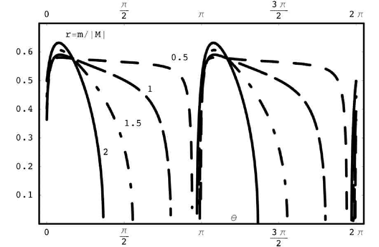
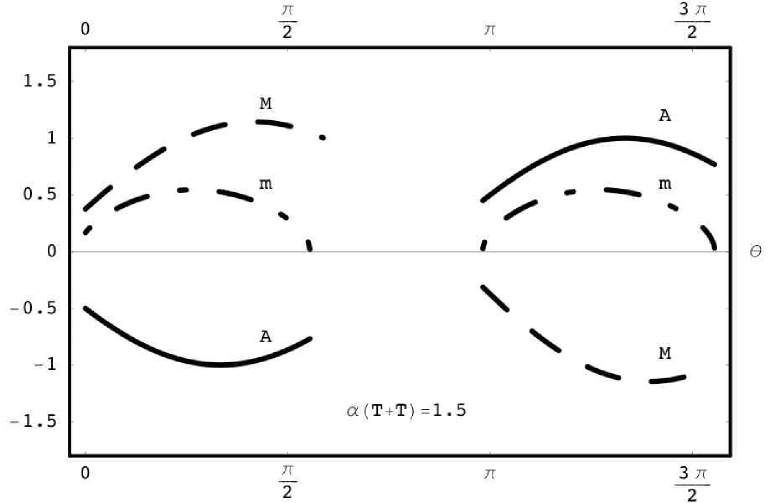
Figure 8: Left : The ratio $r\equiv m/|M|$ as a function of $\theta$ for four different values of $\alpha(T+\bar{T})$ represented by various curves. Right: The universal soft parameters as a function of $\theta$ for $\alpha(T+\bar{T})=1.5$. The solid curve stands for trilinears, dotted dashed curve for scalars and dashed curve for gauginos.

where we are using the following parameterization, which define $F$ terms for the moduli Brignole:1997dp :

$$F^{s} = \sqrt{3}m_{3/2}C(s+\bar{s})\sin(\theta)e^{-i\gamma_{s}}$$ (3)

$$F^{t} = m_{3/2}C(t+\bar{t})\cos(\theta)e^{-i\gamma_{t}}$$

$$C^{2} = 1+\frac{V_{0}}{3m_{3/2}^{2}}$$

The ratio of the scalar to the gaugino mass parameter $r\equiv m/|M|$ is shown in the first plot in Figure 8 as a function of the goldstino angle $\theta$. For the stau coannihilation region, the ratio $r$ has to be roughly $0.5-0.6$. We see that for this value of $r$, one set of allowed values of $\theta$ lie near $0,\pi,2\pi$ for all allowed values of $\alpha(T+\bar{T})$. This means that the supersymmetry breaking is moduli dominated ($F_{s}\approx 0$). In addition, there also exist other values of $\theta$ which are closer to ($\frac{1}{2}\pi,\frac{3}{2}\pi$) rather than to ($0,\pi,2\pi$). However, these values are ruled out by constraints on low energy phenomenology, as the trilinear parameter $A_{0}$ for these values is pretty large, as seen from the second plot in Figure 8. This is because a very large value of the trilinear parameter makes the scalar mass squared run negative at the low scale and also causes problems for EWSB. Once the correct ratio $r$ of the gaugino mass parameter to the scalar mass parameter is obtained, one can get their correct absolute scales by tuning $m_{3/2}$ as all the soft parameters are proportional to them. One thus gets a gluino in the $550-650$ GeV range. The allowed values of $m_{3/2}$ lie in the TeV range.

Moving on to the PH-B construction, one would again like to understand the origin of the characteristic features of its spectrum, viz. heavy squarks ($\geq 1$ TeV), moderately heavy sleptons except the stau which is considerably lighter, and gluinos which can vary from being light ($250-450$ GeV) to heavy ($\geq 1000$ GeV). Light gluinos ($<450$GeV) in this construction always give rise to a wino LSP while the heavier ones give rise to bino or wino LSPs, as we explain below.

The PH-B construction is a weakly coupled heterotic string construction with a tree level Kähler potential and two gaugino condensates. The soft terms for this construction depend on the “theory” input parameters – the gravitino mass $m_{3/2}$, the Green-Schwarz coefficient $\delta_{GS}$ and the $vev$ of the Kähler modulus $t$, in addition to $\tan{\beta}$. In these kind of constructions, it was further noted that a minimum with $F_{s}=0$ and $F_{t}\neq 0$ is preferred with $t$ being stabilized at values slightly greater than 1. For details, refer to Casas:1990qi . The result is that all soft terms are zero at tree level. The expressions for the soft parameters are approximately given by Kane:2002qp :

$$M_{a} \approx \frac{g_{a}^{2}}{2}\,[(2\frac{\delta_{GS}}{16{\pi}^{2}}+b_{a})\,G_{2}(t,\bar{t})+2b_{a}m_{3/2}];\;\;G_{2}(t,\bar{t})\equiv(2\zeta(t)+\frac{1}{t+\bar{t}})$$ (4)

$$m_{i}^{2} \approx \gamma_{i}\,m_{3/2}^{2}$$

$$A_{ijk} \approx m_{3/2}\,(\gamma_{i}+\gamma_{j}+\gamma_{k})$$

where $\zeta(t)$ is the Riemann zeta function. The dominant contribution to the soft scalar mass parameters is proportional to the gravitino mass with the proportionality constant being the anomalous dimension of the respective fields ($\gamma_{i}$). Since the anomalous dimension of the quarks is bigger than that of the leptons, the squarks turn out to be heavier than the sleptons. Also, the anomalous dimension of the stau ($\tilde{\tau}$) is the smallest (smaller by a factor of about 3 compared to that for $\tilde{Q}_{3}$), leading to the stau as the lightest slepton. To get the absolute scale correct, one has to realize that soft terms in this case arise from one loop contributions. Thus, they are suppressed and therefore need a much heavier $m_{3/2}$ $(\sim 20$ TeV) in order to evade the chargino, neutralino and higgs mass lower bounds. This is the reason for the heavy squarks, moderately heavy sleptons and a light stau at the low scale.

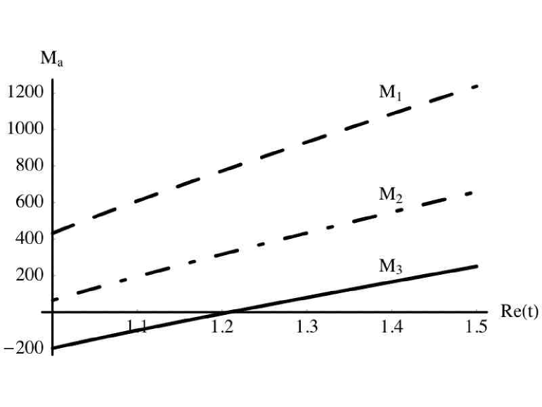
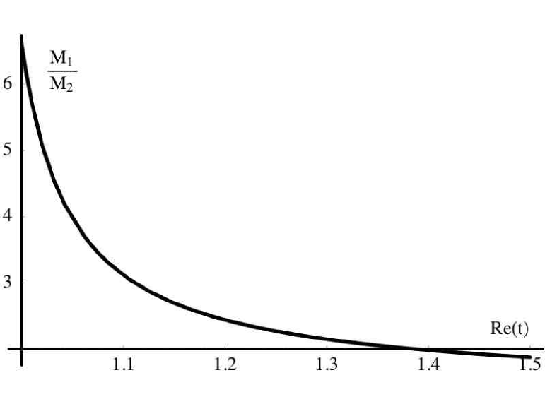
Figure 9: Left : Plots for gaugino mass parameters as a function of Re($t$): The solid curve stands for $M_{3}$, dotted-dashed for $M_{2}$ and dashed for $M_{1}$. Right : The ratio $M_{1}/M_{2}$ as a function of $Re(t)$. Re($t$) varies from 1 to 1.5. The plots are shown for a given value of $\delta_{GS}$ and $m_{3/2}$. $\delta_{GS}$ is -15 and $m_{3/2}$ is 20 TeV.

For the gaugino sector, it is instructive to look at the plots of the variation of gaugino mass parameters as a function of Re($t$) and the ratio of bino and wino mass parameter ($\frac{M_{1}}{M_{2}}$) as functions of Re($t$) for a given value of $\delta_{GS}$ and $m_{3/2}$. Choosing different values of $\delta_{GS}$ does not change the qualitative feature of the plots. Since all gaugino mass parameters are proportional to $m_{3/2}$, changing $m_{3/2}$ changes the overall scale of all gaugino mass parameters. We first explain why light gluinos give rise to a wino LSP while heavier ones to a bino LSP for a fixed $m_{3/2}$. We then consider the effects of changing $m_{3/2}$. The first plot in Figure 9 shows that the gluino mass parameter is the smallest of the three (taking the sign into account) at the unification scale. This arises from the fact that the combination ($G_{2}(t,\bar{t})+2m_{3/2}$) in (4) is negative and the one loop beta function coefficient $b_{3}$ is the largest for $M_{3}$ Kane:2002qp . From the second plot, we see that ratio $\frac{M_{1}}{M_{2}}$ is greater than 2 for Re($t$) smaller than a certain value, which is around 1.4 for the value of $\delta_{GS}$ chosen in the figure. Since we roughly have :

$$M_{1_{low}}\approx 0.45\,M_{1_{unif}};\;\;M_{2_{low}}\approx 0.9\,M_{2_{unif}},$$ (5)

it implies that if the ratio $\frac{M_{1_{unif}}}{M_{2_{unif}}}$ is greater than 2, we have $M_{1_{low}}>M_{2_{low}}$, leading to a wino LSP. Therefore for Re($t$) smaller than a certain value (1.4 in the figure), one obtains a wino LSP while for greater values of Re($t$) one obtains a bino LSP. From the first plot, one now sees that for values of Re($t$) smaller than the critical value, the gluino mass is quite small at the unification scale. Thus for a given $m_{3/2}$, PH-B models with small gluino masses have wino LSPs while those with heavy gluinos have bino LSPs. If we now change the gravitino mass, we change the overall scale of the gaugino mass parameters. Since the scalars are also proportional to $m_{3/2}$, it is not possible to make $m_{3/2}$ very small as the higgs mass bound will be violated. But one can have a large gravitino mass giving rise to a large gluino mass, with both wino and bino LSPs. Bino LSP models however have heavier gluino masses than those with wino LSP as $M_{3}$ is bigger for the bino LSP models, as explained above. One also finds that for Re($t$) around a particular value (1.2 in the above figure), the gluino mass almost vanishes leading to a gluino LSP at the low scale, which is not considered in our analysis. Therefore that region in Re($t$) is not allowed. Another region which is not allowed by low energy constraints is the region near Re($t$)=1, where $M_{2}$ becomes very small, leading to incompatibilities with the lightest chargino and LSP bounds.

VII.5 Explanation of Soft Parameters from the Underlying Theoretical Construction

One finally needs to explain the structure of soft terms (which explains the spectrum pattern and hence the signature pattern) from the structure of the underlying theoretical construction. This would complete the sequence of steps to go from LHC signatures to string theory. As explained before, we carry out this exercise for the KKLT and Large Volume constructions, since they are well defined from a microscopic point of view, and have a reasonably well understood mechanism of supersymmetry breaking and moduli stabilization.

Both of the constructions have complex structure moduli and dilaton stabilized by turning on generic fluxes. The Kähler moduli are stabilized by including non-perturbative corrections to the superpotential. In Large Volume (IIB-L) vacua, a certain kind of $\alpha^{\prime}$ correction is also taken into account in the scalar potential unlike that in the KKLT (IIB-K) vacua. In type IIB-K constructions, the flux superpotential has to be fine-turned so as to give a small ($\sim$ TeV) gravitino mass. For the IIB-L construction however, no fine-tuning of the flux superpotential is required. This gives rise to a relatively low (intermediate scale) string scale if one wants a small gravitino mass.

The common feature of these two constructions is that the Kähler moduli are stabilized mostly by non-peturbative corrections. This leads to a particular feature in the gaugino sector. It was shown in Conlon:2006us that the gaugino masses are suppressed relative to the gravitino mass $(\sim m_{3/2}/\ln(m_{pl}/m_{3/2}))$ in all type IIB vacua with matter residing on stacks of D7-branes and with all Kähler moduli stabilized mostly by non-perturbative corrections to the superpotential.

For the IIB-K constructions studied mostly in the literature, there is only one overall Kähler modulus, the F-term of which is suppressed. Since both the scalar masses and trilinear terms are proportional to this F-term, they are both suppressed relative to the gravitino in the IIB-K construction Choi:2004sx . Anomaly mediated contributions to soft terms have to be added as they are comparable with those at tree level, leading to mixed modulus-anomaly soft supersymmetry breaking terms. The above feature survives for cases with more Kähler moduli, if all of them are stabilized mostly by non-perturbative effects Denef:2005mm . On the other hand, the IIB-L constructions require the presence of a large volume limit – this means that the Calabi-Yau manifold must have at least two Kähler moduli- one of which is small ($T_{s}$) and the other is big ($T_{b}$)Balasubramanian:2005zx . The presence of the perturbative $\alpha^{\prime}$ correction in the Kähler potential gives a contribution to the scalar potential of the same order as the non-perturbative corrections for the “big” Kähler modulus, in contrast to that in the IIB-K construction. The F-term of the small Kähler modulus ($F_{s}$) is suppressed by $\ln(m_{pl}/m_{3/2})$, while that of the big Kähler modulus ($F_{b}$) is not suppressed. Since only D7-branes wrapping the small 4-cycle (represented by the small modulus) give a reasonable gauge coupling, the visible sector gaugino masses are proportional to $F_{s}$ and are suppressed relative to $m_{3/2}$. However both $F_{s}$ and $F_{b}$ enter into the expression for scalar masses and trilinear terms. Since $F_{b}$ is not suppressed, therefore for the IIB-L construction, only the gaugino sector has mixed modulus-anomaly terms, with the scalars and trilinears generically of the same order as the gravitino mass. This characteristic feature is also true for Calabi-Yaus with more Kähler moduli provided they admit a large volume limit, though the explicit soft terms are hard to obtain. Another difference between the IIB-K and IIB-L constructions is that the soft terms for the IIB-K construction are first computed at the unification scale ($\sim 10^{16}$ GeV) while those for the IIB-L construction are computed at the intermediate string scale ($\sim 10^{11}$ GeV).

The above analysis thus explains the origin of the pattern of soft parameters in terms of the structure of the underlying theoretical construction for the two constructions which leads to a distinguishable signature pattern at the LHC. The important thing to take home from this analysis is that different constructions lead to different effective actions and therefore to different expressions for the soft terms in terms of the underlying microscopic input parameters. In addition, the relations among the different soft parameters ($M_{a},m^{2}_{i}\,\&\,A_{ijk}$) also change for different constructions. Therefore, a proper understanding of these relations and their implications for relevant features of the phenomenology is the key to relating high scale theory and data. In this sense, we think that the approach advocated here is likely to work even if one has much more realistic constructions from different parts of the M-theory amoeba which stabilize all the moduli, generate a stable hierarchy and also give a realistic spectrum and couplings.

VIII Distinguishing Theories Qualitatively

In the previous section, we analyzed the eight constructions in great detail – in particular, we computed the LHC signatures of these constructions and understood the origin of these signatures from features of the theoretical constructions. It is worthwhile to ask whether one can abstract important lessons from this exercise so that one could use them to analyze other classes of constructions, and to draw qualitative reliable conclusions from data.

For example, one could try to first extract relevant phenomenological features of the effective beyond-the-Standard Model theory from data and then focus on classes of M theory vacua which give rise to those particular features. This alternative may also be more helpful to people who are interested primarily in understanding general features of beyond-the-Standard Model (BSM) physics from LHC data rather than connecting it to an underlying high scale theory like string theory. From our studies, we find that a combination of features of any construction crucially determine the broad pattern of LHC signatures. For concreteness, we write our results in the framework of low-scale supersymmetry as BSM physics, similar results will hold true for other approaches as well. The important features we find are:

• The universality (or not) of gaugino masses at the unification (or compactification) scale.

• If gauginos are non-universal - the origin of the non-universality, i.e. whether the non-universality is present at tree-level itself as opposed to arising mostly due to one-loop anomaly mediated contributions.

• If gauginos are non-universal - the hierarchy between $M_{1}$, $M_{2}$, $M_{3}$ and $\mu$.

• The relative hierarchy between the scalars and gauginos at the string scale, i.e. whether the scalars are of the same order as the gauginos as opposed to being heavier or lighter than the gauginos.

• Nature and content of the LSP.

• Hierarchy among scalars at the string scale, particularly third family vs the first and second families.

Some comments are in order. These features are not always independent of each other. For example, the hierarchy between $M_{1}$, $M_{2}$ and $M_{3}$ determines the nature of the LSP (combined with a knowledge of $\mu$). Also, if tree-level gaugino masses are small so that non-universality arises only due to the anomaly mediated contributions, then the gauginos are typically suppressed relative to the scalars and the hierarchy between $M_{1}$, $M_{2}$ and $M_{3}$ is fixed. Another important fact which should be kept in mind is that a combination of all the features above gives rise to the observed pattern of LHC signatures, not just a particular one. Therefore, once one obtains data, the task boils down to figuring out the correct combination of “relevant features” which reproduces the data (at least roughly). Let’s explain this with two examples - the HM-A construction and the IIB-L construction. Since we are only concerned with relevant features of the effective BSM theory, all constructions considered can be treated equally.

The HM-A and overlapping HM-B and HM-C constructions have universal gaugino masses at the unification scale and have a bino LSP. They also have scalars of the same order as the gauginos at the unification scale, so RGE effects make the scalars (the third generation in particular) lighter than the gauginos at the low scale. This combination of “relevant features” determines the broad pattern of LHC signatures for these constructions. Since the gauginos are universal at the unification scale, the ratio of $M_{1}$, $M_{2}$ and $M_{3}$ at the low scale is $1:2:7$, which controls the lower bound on the gluino mass and the LSP mass due to experimental constraints on the chargino mass. Also, since scalars are slightly lighter than gluinos at the low scale, both $\tilde{g}\tilde{q}$ and $\tilde{q}\tilde{q}$ pair production are comparable. The fact that the LSP is bino-like is also due to universal gaugino masses as well as the fact that the scalars are comparable to gauginos at the unification scale. A bino LSP can then reduce its relic density by stau coannihilation, which can only happen if the stau is light and almost degenerate with the LSP. All these factors give rise to a very specific set of signature pattern, as analyzed in section VII.3.

In contrast, the IIB-L construction has a different set of “relevant features” which determine its broad pattern of LHC signatures and also allow it to be distinguishable from the other constructions. The gaugino masses are non-universal at the string scale and the scalars are heavier than the gauginos at the low scale. One also a mixed bino-higgsino LSP in this case. Since the scalars are heavier than the gauginos, $\tilde{g}\tilde{g}$ pair production is the dominant production mechanism. Also, the only way to decrease the relic density of a bino-like LSP is to have a significant higgsino fraction as the stau (or stop) coannihilation channel is not open. Again, these features result in a very specific set of signature pattern, as analyzed in section VII.3.

We therefore see that the features mentioned above are crucial in determining the pattern of signatures at the LHC. Having said that, it is important to remember that these features only determine the broad pattern of LHC signatures and one needs more inputs to explain the entire signature pattern in detail.

IX Possible Limitations

One may raise questions about a few aspects of our analysis. The first concerns the sampling of the parameter space of each construction. One may worry that by only considering $\sim$50 models ($\sim$100 for the PH-A construction), the parameter space of each construction is sampled very sparsely and adding more models could qualitatively change the overall signature pattern of the constructions. We think however, that it is reasonable to expect that that is not true.

Figure 10: Plot of number of events with 1 lepton and $\geq$ 2 jets and number of events with opposite sign dileptons and $\geq$ 2 jets, each sampled with $\sim 50$ models, except PH-A ($\sim$100 models).

This is because, as explained in the previous sections, we have outlined the origin of the pattern of signatures of the various constructions on the basis of their spectrum and in turn on the basis of their underlying theoretical setup. Since the dependence of the soft terms on the microscopic input parameters as well as relations between the soft terms are known and have been understood, we expect our results for the pattern table to be robust even when the parameter space is sampled more densely. This will be strictly true only if one understands the theoretical construction well enough so that one has a “representative sample” of the entire parameter space of that construction. We expect this to be true for our constructions. In order to confirm our expectation, we simulated $\sim$400 models for the PH-A construction and $\sim$100 for the IIB-K construction and we found that the results obtained with $\sim$100 (and $\sim$50) models did not change when other models were added in our analysis. This can be seen from Figures 10 and 11 as well as Figures 12 and 13. The other signatures also do not change the final result. In the future, we plan to do a much more comprehensive analysis with a dense sampling of the parameter space for all the other constructions.

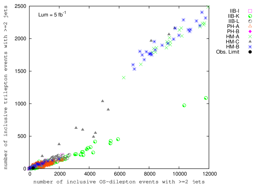
Figure 11: The same plot as in Figure 10, in which the IIB-K construction is sampled with $\sim 100$ models and the PH-A construction with $\sim$400 models.

Another possible objection could be that the procedure of dividing a signature into two classes arbitrarily and distinguishing them on the basis of falling into one class or the other is too naive and may lead to misleading results arising from intrinsic statistical uncertainties and background uncertainties in the value of each signature and impreciseness of the boundary. While this is a valid concern in general, we think that this does not affect the main results of our analysis at this level. This can again be attributed to the fact that the pattern of signatures is understood on the basis of their underlying theoretical structure. We are also encouraged as there are typically more than one (sometimes many) signatures distinguishing any two particular constructions.

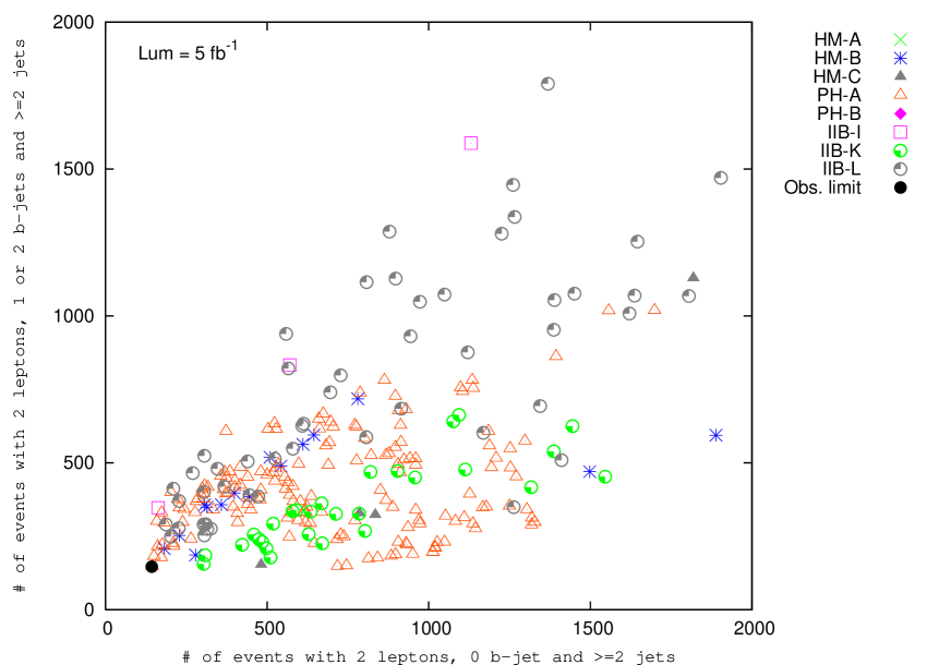
Figure 12: Plot with x axis showing number of events with 2 leptons, 0 b jets and $\geq$2 jets, and y axis showing the number of events with 2 leptons, 1 or 2 b jets and $\geq 2$ jets each sampled with $\sim 50$ models, except PH-A ($\sim$100 models).

Another possible limitation which one could point out is that distinguishing theoretical constructions on the basis of two dimensional signature plots is not very powerful. Since we are only looking at various two-dimensional projections of a multi-dimensional signature space, it is possible that two different theoretical constructions occupy different regions in the multi-dimensional signature space even though they overlap in all the two-dimensional projections. One would then not be able to cleanly distinguish two constructions by this approach even though they are intrinsically distinguishible. However, one can get around this limitation by tagging individual models of each theoretical construction. It would then be possible to figure out if two different constructions are distinguishible even if they overlap in all two dimensional signature plots. As already noted in section V, our purpose was to outline the approach in a simple manner. It is clear that the approach has to be made more sophisticated for more complicated situations.

For a mathematically precise way of distinguishing pairs of constructions, one could use the following procedure. Imagine dividing the parameter space of the two constructions into a coarse grid with coordinates given by their parameter vectors $\vec{x}$. For example, for the PH-A construction, $\vec{x}=\{m_{3/2},a_{np},\tan(\beta)\}$ Kane:2002qp . We can then construct a ${\chi}^{2}$-like variable defined as follows:

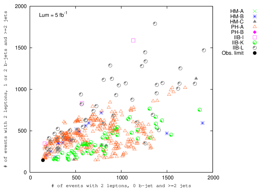
Figure 13: The same plot as in Figure 12, in which the IIB-K construction is sampled with $\sim 100$ models and the PH-A construction with $\sim$400 models.

$$(\Delta S)_{AB}=\mathrm{min}_{\{\vec{x},\vec{y}\}}\sum_{i=1}^{n_{sig}}\left(\frac{s_{A}^{i}(\vec{x})-s_{B}^{i}(\vec{y})}{\sigma_{AB}^{i}}\right)^{2}$$ (6)

where $A$ and $B$ stand for the two constructions, $s_{i}$ stands for the $i$-th signature and $\sigma_{AB}^{i}$ stands for the error bar assigned between the $A$ and $B$ constructions for the $i$-th signature. $\sigma_{AB}^{i}$ can be determined from statistical errors of the $i$-th signature for constructions $A$ and $B$ as well as the standard model background error for the $i$-th signature.

Since we minimize with respect to the parameter vectors $\vec{x}$ and $\vec{y}$ of the two constructions, equation (6) can be geometrically visualized as the “minimum distance squared” in the full multi-dimensional signature space between the two constructions $A$ and $B$ with an appropriate “metric” , and serves as a measure of the difference between the two constructions $A$ and $B$. Carrying out the minimization procedure in practice is quite a non-trivial task, especially when the parameter vectors have many components, as the time required to complete the minimization procedure in a satisfactory way is too large. However techniques have been introduced to get around this problem, for example see Allanach:2004my . In the future, we plan to do a comprehensive analysis with more statistics and a precise method to distinguish models, as explained above.

Finally, one might object to the approach of figuring out experimental predictions for various classes of underlying theoretical constructions and distinguishing different theoretical constructions from each other before actual data, instead of the more “standard” approach of comparing each theoretical construction with actual data. Many reasons can be given in this regard. From a conceptual point of view, this approach fits will with the philosophy of addressing the Inverse Problem in a general framework. It is also crucial to addressing the question of predictivity of an underlying theory like string theory in general and the particular string vacuum we live in, in particular. From a more practical point of view, studying the various subtle aspects of connecting an underlying theoretical construction with collider signatures is quite a non-trivial and subtle exercise and requires considerable time and investment. It is therefore very helpful to build knowledge and intuition in this regard and be prepared for actual data. Carrying out this exercise could help discover important properties of the low-energy implications of various classes of theoretical constructions, in turn pointing to new classes of collider observables as well as helping design new analysis techniques.

X Summary and Future Directions

In this work, we have tried to address the goal of learning about the underlying theory from LHC data - the deeper Inverse Problem. We have proposed an approach by which it can be shown that the two prerequisites to addressing the deeper Inverse Problem, namely, a) To reliably go from a microscopic theory to the space of experimental observables, and b) To distinguish among the various classes of microscopic theoretical constructions on the basis of their experimental signatures, can be satisfied for many semi-realistic string constructions which can be described within the supergravity approximation. In our opinion, the paper is seminal in the sense that it proposes a new way of thinking about fundamental theory, model-building and collider phenomenology such that there is a better synergy between each of these subfields. Perhaps the most important result, which has never before been presented, is that different classes of string constructions give finite footprints in signature space and that different string constructions give practically overlapping but different and distinguishable footprints.

The reason it is possible to distinguish theoretical constructions is that patterns of experimental observables (for eg. signatures at the LHC) are sensitive to the structure of the underlying theoretical constructions, because of correlations (see section VII.2). More precisely, this means that a given theoretical construction occupies a finite region of signature space which is in general different from another theoretical construction. Moreover, the origin of this difference can be understood from the underlying structure of the construction. Therefore, even though we have carried out a simplified analysis in terms of the imposition of cuts, detection efficiencies of particles, detector simulation and calculation of backgrounds, we still have confidence in the robustness of our results. We have analyzed two classes of string vacua and six other string-motivated constructions in detail. The point of this exercise was to illustrate our approach, the same procedure should be carried out for more classes of realistic vacua so that the procedure becomes more-and-more useful. If the approach fails, it will not be because of these and similar issues discussed above, but rather because many regions of the entire M theory amoeba cannot yet be analyzed by the approach we use. However, we think that rather than giving up ahead of time, the best attitude is to continue to expand both theoretical understanding as well as our approach, and confront them with data.

There are two directions in which the approach advocated in this paper can be generalized and sharpened further. The first concerns theoretical issues – efforts should be made to go beyond toy models focussing on few aspects of theory and phenomenology to more holistic ones that address (if not solve) all of the issues an underlying string theoretic construction might be expected to explain. For instance, a better understanding of the theory can fix some (or all) of the microscopic input parameters of a given construction, increasing the predictivity of the construction. The approach advocated by M. Douglas and W. Taylor, viz. to look for correlations in the space of observables by analyzing different classes of vacua is very similar to our approach in principle douglas-taylor .

The second concerns the analysis and interpretation of data and its connection to the underlying theory. Creative thinking is needed in identifying collider observables which more directly probe the key features of the Beyond-the-Standard Model (BSM) lagrangian and its connection to the underlying theory. We were able to identify some useful observables by examining specific constructions. In addition, one should find ways in which observables from all fields – collider physics, flavor physics, cosmology, etc. could be used in conjunction to distinguish among, and favor or exclude, many classes of string constructions in a quick and robust manner. Our proposed technique is very useful in this regard as it is very easy to add non-collider observables – such as from flavor physics, cosmology, etc. to the collider observables such that they are all treated in a uniform manner.

It is important to understand that the proposed approach should be applied at various stages, with different tools and techniques useful for each stage. The first stage would consist of distinguishing many classes of constructions with limited amount of data by using simple signatures and simple analysis techniques. This has the advantage that one can rule out various classes of constructions with relative ease. However, in order to go further, it is important to develop more specialized analysis techniques and use more exclusive signatures. This is best done in subsequent stages, when one zooms in to a more limited set of constructions and also obtains more data. Since one has better statistics, one can use optimized and more exclusive signatures as well as use more sophisticated analysis techniques to get more detailed information about the constructions. Many of these sophisticated analysis techniques already exist in the literature Kneur:1998gy , although they have been applied to very special scenarios like minimal supergravity, minimal gauge mediation, etc. One would now need to apply similar techniques (suitably modified) to the set of constructions consistent with limited data. Also, in the past year, a lot of progress has been made towards uncovering the low energy spectrum and parameters from (simulated) LHC signatures in the form of “blackboxes” constructed by some groups. This has been the program of the LHC Olympics Workshops in the past year LHCO-talks .

Combining these sophisticated techniques with (some) knowledge of the connection between theoretical constructions and data obtained in the first stage, we hope that one can further distinguish the remaining constructions, learn more about underlying theoretical issues, like supersymmetry breaking and mediation, moduli stabilization, inflation, etc.

On a more philosophical note, we understand that in many cases the structure of string theory is not understood well enough to permit a connection to low energy physics in general and collider data in particular. In such a situation, we think that the most useful approach one can take is to compute predictions for low energy experimental observables for as many classes of realistic string vacua as possible and try to learn how information from experimental data may favor some regions of the M-theory amoeba over others. Doing so will lead to learning more about string theory, and could be crucial to learning how or if string theory can be related to the real world.

XI Acknowledgments

The authors appreciate helpful conversations with and suggestions from Marcus Berg, Joseph Lykken, David Morrissey, Brent Nelson, Fernando Quevedo, Michael Schulz, Washington Taylor, Jesse Thaler, Lian-Tao Wang, Ting Wang and James Wells. GLK and PK thank the Kavli Insitute for Theoretical Physics (KITP), UCSB for its hospitality where part of the research was conducted. The research of GLK and PK supported in part by the US Department of Energy and in part by the National Science Foundation under Grant No. PHY99-07949. The research of JS is supported by the US Department of Energy.

Appendix A Description of “String-motivated” Constructions

Here we give a description of the string motivated constructions used in our study. As stated earlier, we work in the framework of string theory giving rise to semi-realistic constructions with low-energy supersymmetry. Taking the extraordinary (apparent) unification of gauge couplings in the MSSM to be an important clue to fundamental physics, we only consider constructions which can lead to unification of gauge couplings. In addition for simplicity, in this paper we assume that the low energy spectrum is that of the MSSM with no intermediate scale physics between the TeV scale and the unification scale.

The constructions used in our study come from different corners of the string/M theory amoeba. As explained in section IV, these constructions are not complete from a theoretical point of view, especially because aspects of moduli stabilization and supersymmetry breaking have not been taken into account in a comprehensive manner. Supersymmetry breaking, for instance, is only parameterized. The constructions are described below:

Weakly coupled Heterotic string constructions

Weakly coupled heterotic string constructions are the oldest branch of string phenomenology, with many papers in the literature Dixon:1986qv . A good review of the subject can be found in Font:1989aj . In most examples of such constructions, one compactifies on a six dimensional toroidal orbifold with $\mathcal{N}=1$ SUSY and calculates the exact spectrum and some couplings. Many examples are known, with a spectrum close to that the MSSM, albeit with some exotics. There are also constructions with compactifications on Calabi-Yaus, although one has less control on the spectrum and couplings. The effective lagrangian thus obtained is given by $\mathcal{N}=1,d=4$ supergravity, which is encoded by three functions - the Kahler potential ($K$), the superpotential ($W$) and the gauge kinetic function ($f$). These functions depend in general on moduli fields which basically parametrize the size and shape of the compactified dimensions. Among the moduli fields is the dilaton which is unique in the sense that it appears at low energies in a uniform way. Its vacuum expectation value gives the value of the string coupling constant ($g_{str}$). For the weakly coupled heterotic string, it also represents the tree level value of the gauge kinetic function.

Constructions with non-perturbative contributions to the Kähler Potential

In this class of constructions, one considers compactification on a toroidal orbifold with $\mathcal{N}=1$ SUSY and a spectrum similar to that of the MSSM. The SUSY breaking mechanism is thought to be provided by the non-perturbative phenomenon of gaugino condensation which generates a non-perturbative superpotential for the dilaton. The susy breaking mechanism in the closed string (moduli) sector is mediated to the visible sector by gravity. However, if one takes the tree level Kähler potential, it is known that one gaugino condensate cannot stabilize the dilaton with vanishing vacuum energy without resorting to strong coupling. In this class of models, one considers a non-perturbative contribution to the Kähler potential á la Shenker:1990uf to get around this problem. Explicit models have been constructed which incorporate this Kähler stabilization mechanism with a realistic model of modular invariant gaugino condensation in the hidden sector Binetruy:1996xj . Instead of constructing explicit detailed models of supersymmetry breaking, one can generate benchmark models by parameterizing the supersymmetry breaking by the F-term for the dilaton and treating the gravitino mass and the nonperturbative contribution to the Kähler potential as tunable parameters (within appropriate ranges) Kane:2002qp .

Constructions with tree level Kähler Potential and multiple gaugino condensates

As in the previous case, one again considers compactification on toroidal orbifolds leading to a semi-realistic spectrum. However, here one considers a tree level Kähler potential with multiple gaugino condensates (typically two) to stabilize the dilaton and break supersymmetry. Supersymmetry breaking is mediated by gravity. In addition, one also has to take into account a Green Schwarz counterterm, which is inherited from the underlying string theory and can be thought of as a loop correction. Explicit models stabilizing the dilaton and the untwisted moduli at reasonable values and giving a gravitino mass of the order of 1-10 TeV have been constructed Casas:1990qi . This typically leads to a minimum with $\langle F^{S}\rangle=0$ and $\langle F^{T_{i}}\rangle\neq 0$. For generating benchmark models, one can take the gravitino mass, the Green-Schwarz coefficient and the vev of the untwisted moduli of the orbifold as tunable parameters (within appropriate ranges). For further details, please refer to Kane:2002qp .

Strongly coupled Heterotic string constructions

In this class of constructions, as the name suggests one looks at the strongly coupled limit of $E_{8}\times E_{8}$ heterotic string theory. Horava and Witten showed that this limit of heterotic string theory can be described by eleven-dimensional supergravity on a manifold with boundaries where the two $E_{8}$ gauge multiplets are restricted to the two ten dimensional boundaries HW1 . So, it is also known as Heterotic M theory, as eleven dimensional supergravity is the low energy description of M theory. To go to four dimensions, one compactifies the eleven dimensional M theory on a Calabi-Yau manifold times an interval. The effective action for this class of constructions, which is again four dimensional $\mathcal{N}=1$ supergravity, has been studied up to the first order in the eleven dimensional parameter $\epsilon$ Witten . Heterotic M theory has some nice phenomenological properties, for eg. it is possible to lower the eleven dimensional Planck scale ($M_{11}$) to the phenomenologically favored scale of unification of the known gauge couplings ($M_{unif}$) in a natural manner BD , thereby achieving a truly unified theory. However, concrete model building such as getting the precise spectrum and couplings and stabilizing all the moduli with the desired properties, is difficult.

Heterotic M theory Constructions with one modulus

The simplest situation occurs when one considers compactification on a Calabi-Yau with Hodge-Betti number $h_{1,1}=1$ and $h_{2,1}=0$, as the relevant expressions are simple. In this class of constructions, the gauge coupling of the $E_{8}$ on the hidden boundary typically becomes large at around the unification scale and so it is reasonable to expect gaugino condensation in the hidden $E_{8}$ sector. This phenomenon breaks supersymmetry which is transmitted to the visible boundary by gravity. For constructing benchmark models, one can parametrize the supersymmetry breaking by F terms for the dilaton ($S$) and the radius modulus of the eleventh dimension ($T$). This gives rise to universal soft terms Choi:1997cm .

Heterotic M theory Constructions with many moduli

Here one considers compactification on a more general Calabi-Yau, with $h_{1,1}>1$, i.e. more than one Kähler modulus. While from a conceptual point of view this should not be treated differently from the previous case, it turns out that from the phenomenological point of view it gives rise to different consequences. The basic reason is that in this case, one loses universality of soft terms. In addition, most of the explicit semi-realistic compactifications with a spectrum similar to that of the MSSM have been on Calabi-Yaus with $h_{1,1}>1$. Therefore, it makes sense to consider this more general case separately. Soft terms have been computed in the supergravity limit for Calabi-Yau compactifications in ten dimensions with more than one Kähler modulus BIMS . Using the above and the general result for the effective action up to the first order in the expansion parameter $\epsilon$, the (numerical) computation of soft parameters can be extended for some Calabi-Yau manifolds with two Kähler moduli jing .

Heterotic M theory Constructions with five-branes

In Heterotic M theory, one has non-perturbative objects called M-5 branes which are sources for the dual of the four-form field strength present in eleven dimensional supergravity. It can be shown that under certain circumstances, these M5 branes survive the orbifold projection of the Horava-Witten construction, permitting much more freedom to play with matter fields, gauge groups and yukawa textures. The functions encoding the effective action of $\mathcal{N}=1$ supergravity taking the effect of five-brane moduli into account have been computed Lukas:1998hk . In this setup, it can also be shown that supersymmetry can still be broken by the same global mechanism (as in the case without five-branes) and is transmitted to the visible sector by gravity. For benchmark models, one can assume supersymmetry braking to be parametrized by F terms for the dilaton, Kähler moduli and the five-brane moduli. An explicit calculation of soft-terms has been done in Cerdeno:1999ur .

Type II String theory Constructions

This class of constructions is relatively more recent than the previously considered heterotic constructions. It has been shown that there exist new classes of perturbative $\mathcal{N}=1$, $D=4$ vacua which have their origin in type II string theory Ibanez:2001jhep . Blumenhagen:2005mu is a good review. The development of D-brane physics is crucial for these constructions. Here one considers type II (A or B) string theory compactified on a six dimensional manifold $X$. For explicit calculations of the couplings, one typically takes $X$ to be a toroidal orientifold, although Calabi-Yau manifolds can also be used in general. In addition, one has various stacks of Dp-branes wrapping different cycles. The spectrum for this setup naturally consists of non-abelian gauge theory coupled to chiral matter. The dependence of the quantities - $K,W,f$ encoding the $\mathcal{N}=1$ effective action on the moduli has been derived for many cases Cvetic:2003ch .

Type II String theory Constructions on toroidal orientifolds with Intersecting D-branes

In type IIA language, in this class of constructions one compactifies on toroidal orientifolds with stacks of intersecting IIA D-branes wrapping intersecting cycles in the compact space. Various examples have been constructed with a spectrum close to that of the MSSM, although with exotics Ibanez:2001jhep . In type IIB language, which is related by T-duality to the previous one, one has background magnetic fluxes on IIB D-brane world volumes. Supersymmetry in type II models can be broken either by strong gauge dynamics in hidden sector D-brane stacks Cvetic:2003yd or by supergravity fluxes gkp01 . The supersymmetry breaking is transmitted to the visible D-brane stacks by gravity, if one assumes that the there is no intersection between the visible and hidden stacks. For benchmark models, one can parametrize the supersymmetry breaking by F terms for the moduli. For concreteness, we will use the soft terms calculated for a particular intersecting D-brane setup in terms of the moduli and their F terms Kane:2004hm . Even though gauge coupling unification is not unified in D-brane models in general, the parameter space can be constrained by imposing such a requirement. This was done in Kane:2004hm .

References

-
(1)
M. Battaglia, A. Datta, A. De Roeck, K. Kong and K. T. Matchev,
JHEP 0507, 033 (2005)
[arXiv:hep-ph/0502041].
J. M. Smillie and B. R. Webber, JHEP 0510, 069 (2005) [arXiv:hep-ph/0507170].
A. Datta, K. Kong and K. T. Matchev, Phys. Rev. D 72, 096006 (2005) [Erratum-ibid. D 72, 119901 (2005)] [arXiv:hep-ph/0509246].
A. Datta, G. L. Kane and M. Toharia, arXiv:hep-ph/0510204.
H. C. Cheng, I. Low and L. T. Wang, arXiv:hep-ph/0510225.
P. Meade and M. Reece, arXiv:hep-ph/0601124. - (2) P. Binetruy, G. L. Kane, B. D. Nelson, L. T. Wang and T. T. Wang, Phys. Rev. D 70, 095006 (2004) [arXiv:hep-ph/0312248].
-
(3)
S. Weinberg,
Phys. Rev. D 13, 974 (1976).
T. W. Appelquist, D. Karabali and L. C. R. Wijewardhana, Phys. Rev. Lett. 57, 957 (1986).
B. Holdom and J. Terning, Phys. Lett. B 247, 88 (1990).
C. T. Hill, Phys. Lett. B 345, 483 (1995) [arXiv:hep-ph/9411426]. M. A. Luty and T. Okui, arXiv:hep-ph/0409274.
T. Appelquist, N. Christensen, M. Piai and R. Shrock, Phys. Rev. D 70, 093010 (2004) [arXiv:hep-ph/0409035].
M. Perelstein, JHEP 0410, 010 (2004) [arXiv:hep-ph/0408072]. -
(4)
N. Arkani-Hamed, S. Dimopoulos and G. R. Dvali,
Phys. Lett. B 429, 263 (1998)
[arXiv:hep-ph/9803315].
N. Arkani-Hamed, S. Dimopoulos and G. R. Dvali, Phys. Rev. D 59, 086004 (1999) [arXiv:hep-ph/9807344].
N. Arkani-Hamed, S. Dimopoulos, G. R. Dvali and J. March-Russell, Phys. Rev. D 65, 024032 (2002) [arXiv:hep-ph/9811448].
N. Arkani-Hamed, S. Dimopoulos, G. R. Dvali and N. Kaloper, Phys. Rev. Lett. 84, 586 (2000) [arXiv:hep-th/9907209].
Phys. Lett. B 436, 257 (1998) [arXiv:hep-ph/9804398].
I. Antoniadis, Phys. Lett. B 246, 377 (1990). -
(5)
L. Randall and R. Sundrum,
Nucl. Phys. B 557, 79 (1999)
[arXiv:hep-th/9810155].
L. Randall and R. Sundrum, Phys. Rev. Lett. 83, 3370 (1999) [arXiv:hep-ph/9905221].
L. Randall and R. Sundrum, Phys. Rev. Lett. 83, 4690 (1999) [arXiv:hep-th/9906064]. -
(6)
Y. Nomura,
JHEP 0311, 050 (2003)
[arXiv:hep-ph/0309189].
C. Csaki, C. Grojean, J. Hubisz, Y. Shirman and J. Terning, Phys. Rev. D 70, 015012 (2004) [arXiv:hep-ph/0310355].
C. Csaki, C. Grojean, H. Murayama, L. Pilo and J. Terning, Phys. Rev. D 69, 055006 (2004) [arXiv:hep-ph/0305237].
C. Csaki, C. Grojean, L. Pilo and J. Terning, Phys. Rev. Lett. 92, 101802 (2004) [arXiv:hep-ph/0308038].
R. S. Chivukula, E. H. Simmons, H. J. He, M. Kurachi and M. Tanabashi, Phys. Lett. B 603, 210 (2004) [arXiv:hep-ph/0408262]. -
(7)
D. B. Kaplan, H. Georgi and S. Dimopoulos,
Phys. Lett. B 136, 187 (1984).
H. Georgi and D. B. Kaplan, Phys. Lett. B 145, 216 (1984).
R. S. Chivukula, C. Hoelbling and N. J. Evans, Phys. Rev. Lett. 85, 511 (2000) [arXiv:hep-ph/0002022].
K. Agashe, R. Contino and A. Pomarol, Nucl. Phys. B 719, 165 (2005) [arXiv:hep-ph/0412089]. -
(8)
N. Arkani-Hamed, A. G. Cohen, E. Katz, A. E. Nelson, T. Gregoire and J. G. Wacker,
JHEP 0208, 021 (2002)
[arXiv:hep-ph/0206020].
N. Arkani-Hamed, A. G. Cohen, E. Katz and A. E. Nelson, JHEP 0207, 034 (2002) [arXiv:hep-ph/0206021].
S. Chang and J. G. Wacker, Phys. Rev. D 69, 035002 (2004) [arXiv:hep-ph/0303001].
M. Schmaltz, JHEP 0408, 056 (2004) [arXiv:hep-ph/0407143].
M. Schmaltz and D. Tucker-Smith, arXiv:hep-ph/0502182. -
(9)
N. Arkani-Hamed and S. Dimopoulos,
JHEP 0506, 073 (2005)
[arXiv:hep-th/0405159].
G. F. Giudice and A. Romanino, Nucl. Phys. B 699, 65 (2004) [Erratum-ibid. B 706, 65 (2005)] [arXiv:hep-ph/0406088].
N. Arkani-Hamed, S. Dimopoulos, G. F. Giudice and A. Romanino, Nucl. Phys. B 709, 3 (2005) [arXiv:hep-ph/0409232]. - (10) S. Kachru, R. Kallosh, A. Linde, and S. P. Trivedi, “De Sitter vacua in string theory.” Phys. Rev. D68 (2003) 046005,
- (11) V. Balasubramanian, P. Berglund, J. P. Conlon and F. Quevedo, “Systematics of moduli stabilisation in Calabi-Yau flux JHEP 0503, 007 (2005) [arXiv:hep-th/0502058]. J. P. Conlon, F. Quevedo and K. Suruliz, “Large-volume flux compactifications: Moduli spectrum and D3/D7 soft JHEP 0508, 007 (2005) [arXiv:hep-th/0505076]. B. C. Allanach, F. Quevedo and K. Suruliz, arXiv:hep-ph/0512081.
- (12) C. P. Burgess, R. Kallosh and F. Quevedo, JHEP 0310, 056 (2003) [arXiv:hep-th/0309187].
-
(13)
K. Choi, A. Falkowski, H. P. Nilles, M. Olechowski and S. Pokorski,
JHEP 0411, 076 (2004)
[arXiv:hep-th/0411066].
K. Choi, A. Falkowski, H. P. Nilles and M. Olechowski, Nucl. Phys. B 718, 113 (2005) [arXiv:hep-th/0503216].
A. Falkowski, O. Lebedev and Y. Mambrini, JHEP 0511, 034 (2005) [arXiv:hep-ph/0507110].
K. Choi, K. S. Jeong, T. Kobayashi and K. i. Okumura, Phys. Lett. B 633, 355 (2006) [arXiv:hep-ph/0508029].
H. Baer, E. K. Park, X. Tata and T. T. Wang, “Collider and dark matter searches in models with mixed modulus-anomaly arXiv:hep-ph/0604253. -
(14)
M.K. Gaillard, B.D. Nelson and Y.-Y. Wu,
Phys. Lett. B 459 (1999) 549.
J. Bagger, T. Moroi and E. Poppitz, JHEP 0004 (2000) 009. -
(15)
F. Quevedo, Talk at KITP:
http://online.itp.ucsb.edu/online/strings06/quevedo/
Private Communication. - (16) J. P. Conlon and F. Quevedo, JHEP 0606, 029 (2006) [arXiv:hep-th/0605141].
-
(17)
B. Acharya, K. Bobkov, G. Kane, P. Kumar and D. Vaman,
Phys. Rev. Lett. 97, 191601 (2006)
[arXiv:hep-th/0606262].
B. S. Acharya, K. Bobkov, G. L. Kane, P. Kumar and J. Shao, arXiv:hep-th/0701034. - (18) A. Djouadi, J. L. Kneur and G. Moultaka, [arXiv:hep-ph/0211331].
- (19) B. C. Allanach, Comput. Phys. Commun. 143, 305 (2002) [arXiv:hep-ph/0104145].
-
(20)
C. L. Bennett et al.,
Astrophys. J. Suppl. 148, 1 (2003)
[arXiv:astro-ph/0302207].
D. N. Spergel et al. [WMAP Collaboration], Astrophys. J. Suppl. 148, 175 (2003) [arXiv:astro-ph/0302209]. -
(21)
K. Abe et al. [Belle Collaboration],
Phys. Lett. B 511, 151 (2001)
[arXiv:hep-ex/0103042].
D. Cronin-Hennessy et al. [CLEO Collaboration], Phys. Rev. Lett. 87, 251808 (2001) [arXiv:hep-ex/0108033].
R. Barate et al. [ALEPH Collaboration], Phys. Lett. B 429, 169 (1998). -
(22)
G. W. Bennett et al. [Muon g-2 Collaboration],
Phys. Rev. Lett. 89, 101804 (2002)
[Erratum-ibid. 89, 129903 (2002)]
[arXiv:hep-ex/0208001].
G. W. Bennett et al. [Muon g-2 Collaboration], Phys. Rev. Lett. 92, 161802 (2004) [arXiv:hep-ex/0401008]. - (23) T. Sjostrand, L. Lonnblad, S. Mrenna and P. Skands, LU TP 06-13, FERMILAB-PUB-06-052-CD-T [hep-ph/0603175].
- (24) http://www.physics.ucdavis.edu/ conway/research/software/pgs/pgs4-general.htm.
-
(25)
http://physics.princeton.edu/ verlinde/research/lhco/
http://ph-dep-th.web.cern.ch/ph-dep-th/lhcOlympics/lhcolympicsII.html.
http://www.phys.washington.edu/users/strasslr/LHCO.BBpage.html. -
(26)
H. Baer, C. h. Chen, F. Paige and X. Tata,
Phys. Rev. D 53, 6241 (1996)
[arXiv:hep-ph/9512383].
H. Baer, C. h. Chen, F. Paige and X. Tata, Phys. Rev. D 52, 2746 (1995) [arXiv:hep-ph/9503271]. - (27) N. Arkani-Hamed, G. L. Kane, J. Thaler and L. T. Wang, JHEP 0608, 070 (2006) [arXiv:hep-ph/0512190].
- (28) A. Bartl, W. Majerotto and W. Porod, Z. Phys. C 64, 499 (1994) [Erratum-ibid. C 68, 518 (1995)].
- (29) K. Choi, H. B. Kim and C. Munoz, Phys. Rev. D 57, 7521 (1998) [arXiv:hep-th/9711158].
-
(30)
J. R. Ellis, K. A. Olive, Y. Santoso and V. C. Spanos,
Phys. Lett. B 565, 176 (2003)
[arXiv:hep-ph/0303043].
J. L. Feng, eConf C0307282, L11 (2003) [arXiv:hep-ph/0405215]. - (31) A. Brignole, L. E. Ibanez and C. Munoz, arXiv:hep-ph/9707209.
-
(32)
J. A. Casas, Z. Lalak, C. Munoz and G. G. Ross,
Nucl. Phys. B 347, 243 (1990).
B. de Carlos, J. A. Casas and C. Munoz, Nucl. Phys. B 399, 623 (1993) [arXiv:hep-th/9204012].
B. de Carlos, J. A. Casas and C. Munoz, Phys. Lett. B 299, 234 (1993) [arXiv:hep-ph/9211266].
A. de la Macorra and G. G. Ross, Nucl. Phys. B 404, 321 (1993) [arXiv:hep-ph/9210219]. - (33) F. Denef, M. R. Douglas, B. Florea, A. Grassi and S. Kachru, arXiv:hep-th/0503124.
- (34) G. L. Kane, J. D. Lykken, S. Mrenna, B. D. Nelson, L. T. Wang and T. T. Wang, Phys. Rev. D 67, 045008 (2003) [arXiv:hep-ph/0209061].
- (35) B. C. Allanach, D. Grellscheid and F. Quevedo, JHEP 0407, 069 (2004) [arXiv:hep-ph/0406277].
-
(36)
M. R. Douglas and W. Taylor,
arXiv:hep-th/0606109.
Talk at KITP : http://online.itp.ucsb.edu/online/strings06/taylor/
Private Communication. -
(37)
J. L. Kneur and G. Moultaka,
Phys. Rev. D 59, 015005 (1999)
[arXiv:hep-ph/9807336].
A. Djouadi et al. [MSSM Working Group], arXiv:hep-ph/9901246.
J. L. Kneur and G. Moultaka, Phys. Rev. D 61, 095003 (2000) [arXiv:hep-ph/9907360].
C. G. Lester, M. A. Parker and M. J. White, JHEP 0601, 080 (2006) [arXiv:hep-ph/0508143].
J. A. Aguilar-Saavedra et al., arXiv:hep-ph/0511344.
B. C. Allanach et al., arXiv:hep-ph/0602198. -
(38)
http://physics.princeton.edu/ verlinde/research/lhco/
http://ph-dep-th.web.cern.ch/ph-dep-th/lhcOlympics/2ndWin06/program.html -
(39)
L. J. Dixon, D. Friedan, E. J. Martinec and S. H. Shenker,
Nucl. Phys. B 282, 13 (1987);
S. Hamidi and C. Vafa, Nucl. Phys. B 279, 465 (1987);
I. Antoniadis, J. R. Ellis, J. S. Hagelin and D. V. Nanopoulos, Phys. Lett. B 231, 65 (1989);
G. Cleaver, M. Cvetic, J. R. Espinosa, L. L. Everett, P. Langacker and J. Wang, Phys. Rev. D 59, 115003 (1999) [arXiv:hep-ph/9811355];
G. B. Cleaver, A. E. Faraggi, D. V. Nanopoulos and J. W. Walker, Mod. Phys. Lett. A 15, 1191 (2000) [arXiv:hep-ph/0002060];
L. J. Dixon, V. Kaplunovsky and J. Louis, Nucl. Phys. B 329, 27 (1990);
L. J. Dixon, V. Kaplunovsky and J. Louis, Nucl. Phys. B 355, 649 (1991);
L. E. Ibanez and D. Lust, Nucl. Phys. B 382, 305 (1992) [arXiv:hep-th/9202046];
H. P. Nilles and S. Stieberger, Nucl. Phys. B 499, 3 (1997) [arXiv:hep-th/9702110].
P. Binetruy, M. K. Gaillard and B. D. Nelson, Nucl. Phys. B 604, 32 (2001) [arXiv:hep-ph/0011081]. - (40) A. Font, L. E. Ibanez, F. Quevedo and A. Sierra, Nucl. Phys. B 331, 421 (1990).
-
(41)
S. H. Shenker,
RU-90-47
Presented at the Cargese Workshop on Random Surfaces, Quantum
Gravity and Strings, Cargese, France, May 28 - Jun 1, 1990
J. Polchinski, Phys. Rev. D 50, 6041 (1994) [arXiv:hep-th/9407031].
E. Silverstein, Phys. Lett. B 396, 91 (1997) [arXiv:hep-th/9611195]. -
(42)
P. Binetruy, M. K. Gaillard and Y. Y. Wu,
Nucl. Phys. B 481, 109 (1996)
[arXiv:hep-th/9605170].
P. Binetruy, M. K. Gaillard and Y. Y. Wu, Nucl. Phys. B 493, 27 (1997) [arXiv:hep-th/9611149].
P. Binetruy, M. K. Gaillard and Y. Y. Wu, Phys. Lett. B 412, 288 (1997) [arXiv:hep-th/9702105]. -
(43)
P. Horava and E. Witten, Nucl. Phys. B 460 (1996)
506.
P. Horava and E. Witten, Nucl. Phys. B 475(1996) 94.
P. Horava, Phys. Rev. D 54(1996) 7561. -
(44)
E. Witten, Nucl. Phys. B
471(1996) 135.
A. Lukas, B. A. Ovrut and D. Waldram, Nucl. Phys. B 532, 43 (1998) [arXiv:hep-th/9710208].
A. Lukas, B. A. Ovrut, D. Waldram, JHEP 9904 (1999) 009. -
(45)
T. Banks and M. Dine, Nucl. Phys. B 479 (1996) 137.
T. Banks and M. Dine, arXiv:hep-th/9609046. -
(46)
A. Brignole, L.E. Ibáñez, C. Muñoz and C. Scheich,
Z. Phys. C74 (1997) 157.
H. B. Kim and C. Muñoz, Z. Phys. C 75 (1997) 367. - (47) G.L. Kane, P. Kumar and J. Shao, To appear.
-
(48)
A. Lukas, B. A. Ovrut and D. Waldram,
Phys. Rev. D 59, 106005 (1999)
[arXiv:hep-th/9808101].
A. Lukas, B. A. Ovrut and D. Waldram, Fortsch. Phys. 48, 167 (2000) [arXiv:hep-th/9903144]. -
(49)
D. G. Cerdeno and C. Munoz,
Phys. Rev. D 61, 016001 (2000)
[arXiv:hep-ph/9904444].
D. G. Cerdeno and C. Munoz, Phys. Rev. D 66, 115007 (2002) [arXiv:hep-ph/0206299]. -
(50)
L. E. Ibanez, F. Marchesano and R. Rabadan, JHEP 0111, 002
(2001) [arXiv:hep-th/0105155];
C. Angelantonj and A. Sagnotti, Phys. Rept. 371 (2002) 1 [Erratum-ibid. 376 (2003) 339] [hep-th/0204089].
R. Blumenhagen, L. Görlich and B. Körs, Nucl. Phys. B 569 (2000) 209 [hep-th/9908130];
R. Blumenhagen, L. Görlich and B. Körs, JHEP 0001 (2000) 040 [hep-th/9912204].
G. Pradisi, Nucl. Phys. B 575 (2000) 134 [hep-th/9912218].
R. Blumenhagen, L. Görlich and B. Körs, hep-th/0002146.
C. Angelantonj, I. Antoniadis, E. Dudas and A. Sagnotti, Phys. Lett. B 489 (2000) 223 [hep-th/0007090].
S. Förste, G. Honecker and R. Schreyer, Nucl. Phys. B 593 (2001) 127 [hep-th/0008250].
C. Angelantonj and A. Sagnotti, hep-th/0010279.
S. Förste, G. Honecker and R. Schreyer, JHEP 0106 (2001) 004 [hep-th/0105208].
Nucl. Phys. B 616, 3 (2001) [arXiv:hep-th/0107138];
G. Shiu and S. H. H. Tye, Phys. Rev. D 58, 106007 (1998) [arXiv:hep-th/9805157];
M. Cvetic, P. Langacker and G. Shiu, Phys. Rev. D 66, 066004 (2002) [arXiv:hep-ph/0205252];
D. Lust and S. Stieberger, [arXiv:hep-th/0302221];
I. Antoniadis, E. Kiritsis and T. N. Tomaras, Phys. Lett. B 486, 186 (2000) [arXiv:hep-ph/0004214];
D. Cremades, L. E. Ibanez and F. Marchesano, JHEP 0207, 009 (2002) [arXiv:hep-th/0201205];
R. Blumenhagen, D. Lust and S. Stieberger, JHEP 0307, 036 (2003) [arXiv:hep-th/0305146];
D. Cremades, L. E. Ibanez and F. Marchesano, JHEP 0307, 038 (2003) [arXiv:hep-th/0302105];
F. Marchesano, JHEP 0405, 079 (2004) [arXiv:hep-th/0404229];
M. Cvetic and I. Papadimitriou, Phys. Rev. D 68, 046001 (2003) [Erratum-ibid. D 70, 029903 (2004)] [arXiv:hep-th/0303083];
S. A. Abel and A. W. Owen, Nucl. Phys. B 682, 183 (2004) [arXiv:hep-th/0310257]; Nucl. Phys. B 664, 3 (2003)[arXiv:hep-th/0303124];
B. Kors and P. Nath, Nucl. Phys. B 681, 77 (2004) [arXiv:hep-th/0309167];
D. Lust, P. Mayr, R. Richter and S. Stieberger, Nucl. Phys. B 696, 205 (2004) [arXiv:hep-th/0404134].
I. Antoniadis, E. Kiritsis, J. Rizos and T. N. Tomaras, Nucl. Phys. B 660, 81 (2003) [arXiv:hep-th/0210263].
P. Anastasopoulos, T. P. T. Dijkstra, E. Kiritsis and A. N. Schellekens, arXiv:hep-th/0605226. - (51) R. Blumenhagen, M. Cvetic, P. Langacker and G. Shiu, [arXiv:hep-th/0502005].
-
(52)
M. Bertolini, M. Billo, A. Lerda, J. F. Morales and R. Russo,
Nucl. Phys. B 743, 1 (2006) [arXiv:hep-th/0512067].
M. Cvetic and I. Papadimitriou, Phys. Rev. D 68, 046001 (2003) [Erratum-ibid. D 70, 029903 (2004)] [arXiv:hep-th/0303083];
D. Cremades, L. E. Ibanez and F. Marchesano, JHEP 0307, 038 (2003) [arXiv:hep-th/0302105].
D. Lust, P. Mayr, R. Richter and S. Stieberger, Nucl. Phys. B 696, 205 (2004) [arXiv:hep-th/0404134]; - (53) M. Cvetic, P. Langacker and J. Wang, Phys. Rev. D 68, 046002 (2003) [arXiv:hep-th/0303208].
-
(54)
S. B. Giddings, S. Kachru, and J. Polchinski, “Hierarchies from
fluxes in
string compactifications,” Phys. Rev. D66 (2002) 106006;
P. G. Cámara, L. E. Ibáñez, and A. M. Uranga, “Flux-induced SUSY-breaking soft terms;” Nucl. Phys. B689 (2004) 195–242;
J. Louis, “Soft supersymmetry breaking in Calabi-Yau orientifolds with D-branes and fluxes,” Nucl. Phys. B690 (2004) 21–61;
P. G. Cámara, L. E. Ibáñez, and A. M. Uranga, “Flux-induced SUSY-breaking soft terms on D7-D3 brane systems;”
M. Cvetič, T. Li, and T. Liu, “Standard-like Models as Type IIB Flux Vacua;” - (55) G. L. Kane, P. Kumar, J. D. Lykken and T. T. Wang, Phys. Rev. D 71, 115017 (2005) [arXiv:hep-ph/0411125].