Static properties and semileptonic decays of doubly heavy baryons in a nonrelativistic quark model.

Abstract

We evaluate static properties and semileptonic decays for the ground state of doubly heavy $\Xi,\,\Xi^{\prime},\,\Xi^{*}$ and $\Omega,\,\Omega^{\prime},\,\Omega^{*}$ baryons. Working in the framework of a nonrelativistic quark model, we solve the three–body problem by means of a variational ansatz made possible by heavy quark spin symmetry constraints. To check the dependence of our results on the inter-quark interaction we use five different quark-quark potentials that include a confining term plus Coulomb and hyperfine terms coming from one–gluon exchange. Our results for static properties (masses, charge radii and magnetic moments ) are, with a few exceptions for the magnetic moments, in good agreement with a previous Faddeev calculation. Our much simpler wave functions are used to evaluate semileptonic decays of doubly heavy $\Xi,\Xi^{\prime}(J=1/2)$ and $\Omega,\Omega^{\prime}(J=1/2)$ baryons. Our results for the decay widths are in good agreement with calculations done within a relativistic quark model in the quark–diquark approximation.

I Introduction

Baryon	$S$	$J^{P}$	$I$	$S_{h}^{\pi}$	Quark content
$\Xi_{cc}$	0	$\frac{1}{2}^{+}$	$\frac{1}{2}$	$1^{+}$	$ccl$
$\Xi^{*}_{cc}$	0	$\frac{3}{2}^{+}$	$\frac{1}{2}$	$1^{+}$	$ccl$
$\Omega_{cc}$	$-1$	$\frac{1}{2}^{+}$	0	$1^{+}$	$ccs$
$\Omega^{*}_{cc}$	$-1$	$\frac{3}{2}^{+}$	$0$	$1^{+}$	$ccs$
$\Xi_{bb}$	0	$\frac{1}{2}^{+}$	$\frac{1}{2}$	$1^{+}$	$bbl$
$\Xi^{*}_{bb}$	0	$\frac{3}{2}^{+}$	$\frac{1}{2}$	$1^{+}$	$bbl$
$\Omega_{bb}$	$-1$	$\frac{1}{2}^{+}$	0	$1^{+}$	$bbs$
$\Omega^{*}_{bb}$	$-1$	$\frac{3}{2}^{+}$	$0$	$1^{+}$	$bbs$
$\Xi^{\prime}_{bc}$	0	$\frac{1}{2}^{+}$	$\frac{1}{2}$	$0^{+}$	$bcl$
$\Xi_{bc}$	0	$\frac{1}{2}^{+}$	$\frac{1}{2}$	$1^{+}$	$bcl$
$\Xi^{*}_{bc}$	0	$\frac{3}{2}^{+}$	$\frac{1}{2}$	$1^{+}$	$bcl$
$\Omega^{\prime}_{bc}$	$-1$	$\frac{1}{2}^{+}$	0	$0^{+}$	$bcs$
$\Omega_{bc}$	$-1$	$\frac{1}{2}^{+}$	0	$1^{+}$	$bcs$
$\Omega^{*}_{bc}$	$-1$	$\frac{3}{2}^{+}$	$0$	$1^{+}$	$bcs$

Table 1: Quantum numbers of doubly heavy baryons analyzed in this study. $S$, $J^{P}$ are strangeness and the spin parity of the baryon, $I$ is the isospin, and $S_{h}^{\pi}$ is the spin parity of the heavy degrees of freedom. $l$ denotes a light $u$ or $d$ quark .

The subject of doubly heavy baryons has been attracting attention for a long time. Magnetic moments of doubly charmed baryons were evaluated back in the 70’s by Lichtenberg lichtenberg77 within a nonrelativistic approach. The infinite heavy quark mass limit was already used in the 90’s to relate the spectrum of doubly heavy baryons to the one of mesons with a single heavy quark savage90 , or to analyze their semileptonic decay white91 . A factor of two error in the hyperfine splittings of Ref. savage90 have been recently noticed by the potential nonrelativistic QCD (pNRQCD) calculation of Ref. brambilla05 .

On the experimental side the SELEX Collaboration claimed evidence for the $\Xi^{+}_{cc}$ baryon, in the $\Lambda_{c}^{+}K^{-}\pi^{+}$ and $pD^{+}K^{-}$ decay modes, with a mass of $M_{\Xi^{+}_{cc}}=3519\pm 1\ \mathrm{MeV/c^{2}}$ mattson02 . Those results were challenged by a theoretical analysis kili which claimed the observed events by the SELEX Collaboration could be explained without the involvement of doubly charmed baryons. Other experimental collaborations like FOCUS focus03 , BABAR  babar06 and BELLE lesiak06 have found no evidence for doubly charmed baryons so far. At present the $\Xi^{+}_{cc}$ has only a one star status and it is not listed in the particle summary table pdg06 .

In hadrons with a heavy quark and working in the infinite heavy quark mass limit the dynamics of the light degrees of freedom becomes independent of the heavy quark flavor and spin. This is known as heavy quark symmetry (HQS) hqs1 ; hqs2 ; hqs3 ; hqs4 . This symmetry was developed into an effective theory (HQET) georgi90 that allowed a systematic, order by order, evaluation of corrections in inverse powers of the heavy quark masses. Unfortunately ordinary HQS can not be applied directly to hadrons containing two heavy quarks as the kinetic energy term needed in those systems to regulate infrared divergences breaks heavy flavor symmetry thacker91 . For those hadrons the symmetry that survives is heavy quark spin symmetry (HQSS) jenkins93 , which amounts to the decoupling of the heavy quark spins in the infinite heavy quark mass limit. In that limit one can consider the total spin of the two heavy quark subsystem ($S_{h}$) to be well defined. In this work we shall assume this is a good approximation for the actual heavy quark masses. This approximation, which is the only one related to the infinite heavy quark mass limit that we shall use, will certainly simplify the solution of the baryon three–quark problem. Recently the authors of Ref. brambilla05 have developed and effective theory (pNRQCD) suitable to describe baryons with two and three heavy quarks.

Solving the three–body problem is not an easy task and here we shall do it by means of a variational approach. The approach, with obvious changes, was already applied with good results in the study of baryons with one heavy quark conrado04 . This method, that leads to simple and manageable wave functions, is made possible by the simplifications introduced in the problem by the fact that we can consider $S_{h}$ to be well defined. We shall consider several simple phenomenological quark–quark interactions BD81 ; SS94 ; Si96 which free parameters have been adjusted in the meson sector and are thus free of three–body ambiguities. The use of different interactions will allow us to estimate part of the theoretical uncertainties affecting our calculation. Uncertainties related to the nonrelativistic baryon states that we use are difficult to estimate. We are aware of the limitations of a non-relativistic approach to describe light quark physics. However, for the kind of study performed in this work these are likely not as relevant as in other contexts. We study the semileptonic decays of double heavy baryons, in which the light quark is merely an spectator (heavy-to-heavy transitions). Indeed the lack of a proper relativistic treatment did prevent us to study semileptonic transitions of the type $b\to u$ of a greater phenomenological interest. One should notice however that at least part of the relativistic effects not explicitly taken into account are included in an effective way in the parameters of the interaction which had been fitted to experimental data. We think this explains why the nonrelativistic quark model is so successful phenomenologically even in the presence of light quarks.

Our simple variational calculation reproduces the results for static properties obtained in Ref. Si96 by solving more involved Faddeev type equations. Our method has the advantage that we provide explicit and manageable wave functions that can be used to evaluate further observables. Static properties like masses and magnetic moments of doubly heavy baryons have also been studied in other models. Masses have been calculated in the relativistic quark model assuming a light quark heavy diquark structure ebert02 , the potential approach and sum rules of QCD kiselev02 , the nonperturbative QCD approach narodetskii02 , the Bethe–Salpeter equation applied to the light quark heavy diquark tong00 , the nonrelativistic quark model with harmonic oscillator potential itoh00 or with the use of QCD derived potentials vijande04 ; gershtein00 , the relativistic quasi–potential quark model ebert97 , with the use of the Feynman-Hellman theorem and semi-empirical mass formulas within the framework of a nonrelativistic constituent quark model roncaglia95 , in effective field theories korner94 ; brambilla05 , or in lattice nonrelativistic QCD mathur02 . There are also lattice QCD determinations  khan00 ; lewis01 ; flynn03 . Similarly, magnetic moments have been evaluated in a nonrelativistic approach lichtenberg77 , in the relativistic three–quark model faessler06 , the relativistic quark model using different forms of the relativistic kinematics bruno04 , in the skyrmion model oh91 , in the Dirac equation formalism jena86 , or using the MIT bag model bose80 .

We shall further use our manageable wave functions to study semileptonic decays of doubly heavy , $J=1/2$, baryons. We shall evaluate form factors, decay widths and angular asymmetry parameters. Previous calculations of semileptonic decay widths have been done in different relativistic quark model approaches  ebert04 ; faessler01 ; guo98 , or with the use of HQET sanchis95 .

The paper is organized as follows. In Sect. II we study the Hamiltonian of the system (Subsect. II.1) and briefly introduce the different inter-quark interactions used in this work (Subsect. II.2). The variational wave functions are discussed in Sect. III. In Sect. IV we present results for the static properties: masses (Subsect. IV.1), charge densities and radii (Subsect. IV.2), and magnetic moments (Subsect. IV.3). Semileptonic decays are analyzed in Sect. V. After the presentation of general formulas, in Subsect. V.1 we relate the form factors to matrix elements and show how the latter ones are evaluated within our model. In Subsect. V.2 we present our results for the form factors, differential and total semileptonic decay widths, and angular asymmetry parameters. The findings of this work are summarized in Sect. VI. The paper also includes three appendices: in appendix  A we analyze the infinite heavy quark mass limit of our radial wave functions. In appendix B we relate the form factors for semileptonic decay to the two basic integrals in terms of which all of them can be obtained. Finally, in appendix C we give explicit expressions for those basic integrals.

In Table 1 we summarize the quantum numbers of the doubly heavy baryons considered in this study.

II Three Body Problem

II.1 Intrinsic Hamiltonian

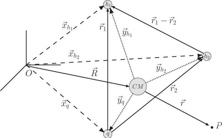
Figure 1: Definition of different coordinates used throughout this work.

In the Laboratory (LAB) frame (see Fig. 1), the Hamiltonian ($H$) of the three quark ($h_{1},\,h_{2},\,q$, where $h_{1},\,h_{2}=c,b$ and $q=l(u,\,d),\,s$) system reads:

$$H = \sum_{j=h_{1},\,h_{2},\,q}\left(m_{j}-\frac{\stackrel{{\scriptstyle\rightarrow}}{{\nabla}}\stackrel{{\scriptstyle}}{{{}^{2}}}_{\vec{x}_{j}}}{2m_{j}}\right)+V_{h_{1}h_{2}}+V_{h_{1}q}+V_{h_{2}q}$$ (1)

where $m_{h_{1}},\,m_{h_{2}},\,m_{q}$ are the quark masses and the quark-quark interaction terms $V_{jk}$ depend on the quark spin-flavor quantum numbers and the quark coordinates ($\vec{x}_{h_{1}},\vec{x}_{h_{2}},\,\vec{x}_{q}$ for the $h_{1},\,h_{2},\,q$ quarks respectively). To separate the Center of Mass (CM) free motion, we go to the light quark frame ($\vec{R},\vec{r}_{1},\vec{r}_{2}$),

$$\vec{R} = \frac{m_{h_{1}}\vec{x}_{h_{1}}+m_{h_{2}}\vec{x}_{h_{2}}+m_{q}\vec{x}_{q}}{m_{h_{1}}+m_{h_{2}}+m_{q}}$$

$$\vec{r}_{1} = \vec{x}_{h_{1}}-\vec{x}_{q}$$

$$\vec{r}_{2} = \vec{x}_{h_{2}}-\vec{x}_{q}$$ (2)

where $\vec{R}$ and $\vec{r}_{1},\,\vec{r}_{2}$ are the CM position in the LAB frame and the relative positions of the $h_{1},\,h_{2}$ heavy quarks with respect to the light quark $q$. The Hamiltonian now reads

$$H = -\frac{\stackrel{{\scriptstyle\rightarrow}}{{\nabla}}\stackrel{{\scriptstyle}}{{{}^{2}}}_{\vec{R}}}{2\overline{M}}+H^{\rm int}$$ (3)

$$H^{\rm int} = \overline{M}+\sum_{j=1,2}\,H_{j}^{sp}+V_{h_{1}h_{2}}(\vec{r}_{1}-\vec{r}_{2},\,spin)-\frac{\stackrel{{\scriptstyle\rightarrow}}{{\nabla}}_{1}\cdot\stackrel{{\scriptstyle\rightarrow}}{{\nabla}}_{2}}{m_{q}}$$

$$H_{j}^{sp} = -\frac{\stackrel{{\scriptstyle\rightarrow}}{{\nabla}}\stackrel{{\scriptstyle}}{{{}^{2}}}_{j}}{2\mu_{j}}+V_{h_{j}q}(\vec{r}_{j},\,spin),\ j=1,2$$ (4)

where $\overline{M}=m_{h_{1}}+m_{h_{2}}+m_{q}$, $\mu_{j}=\left(1/m_{h_{j}}+1/m_{q}\right)^{-1}$ and $\stackrel{{\scriptstyle\rightarrow}}{{\nabla}}_{j}=\partial/\partial_{\vec{r}_{j}},\ j=1,2$. The intrinsic Hamiltonian $H^{\rm int}$ describes the dynamics of the baryon. Apart from the sum of the quark masses $\overline{M}$, it consists of the sum of two single particle Hamiltonian $H^{sp}_{j}$, each of them describing the dynamics of a heavy-light quark system, plus the heavy–heavy interaction term, including the Hughes-Eckart term ($\stackrel{{\scriptstyle\rightarrow}}{{\nabla}}_{1}\cdot\stackrel{{\scriptstyle\rightarrow}}{{\nabla}}_{2}$). We will use a variational approach to solve it.

II.2 Quark–Quark Interactions

We have examined five different interactions, one suggested by Bhaduri and collaborators BD81 (BD) and four suggested by B. Silvestre-Brac and C. Semay Si96 ; SS94 (AL1, AL2, AP1 y AP2). All of them contain a confinement term, plus Coulomb and hyperfine terms coming from one-gluon exchange, and differ from each other in the form factors used for the hyperfine terms, the power of the confining term or the use of a form factor in the one gluon exchange Coulomb potential. All free parameters in the potentials had been adjusted to reproduce the light ($\pi$, $\rho$, $K$, $K^{*}$, etc.) and heavy-light ($D$, $D^{*}$, $B$, $B^{*}$, etc.) meson spectra. All details on the above interactions can be found in Refs. BD81 ; Si96 ; SS94 .

These interactions were also used in Ref. Si96 to obtain, within a Faddeev calculation, the spectrum and static properties of heavy baryons. Our simpler variational method will not only give equally good results for the observables analyzed in Si96 , but it will also provide us with easy to handle wave functions that can be used to evaluate other observables.

III Variational Wave Functions

For the above mentioned interactions, we have that both the total spin and the internal orbital angular momentum given as

$${\vec{S}} = \left({\vec{\sigma}}_{h_{1}}+{\vec{\sigma}}_{h_{2}}+{\vec{\sigma}}_{q}\right)/2$$

$${\vec{L}} = {\vec{l}}_{1}+{\vec{l}}_{2},\qquad{\rm with}~{}~{}{\vec{l}}_{j}=-{\rm i}~{}~{}{\vec{r}}_{j}\times{\stackrel{{\scriptstyle\rightarrow}}{{\nabla}}}_{j},\quad j=1,2$$ (5)

commute with the intrinsic Hamiltonian and are thus well defined. We are interested in the ground state of baryons with total angular momentum $J=1/2,\,3/2$ so that we can assume the orbital angular momentum of the baryons to be $L=0$. This implies that the spatial wave function can only depend on the relative distances $r_{1}$, $r_{2}$ and $r_{12}=|\vec{r}_{1}-\vec{r}_{2}|$. Furthermore when the heavy quark mass is infinity ($m_{h}\to\infty$), the total spin of the heavy degrees of freedom, $\vec{S}_{\rm heavy}=\left({\vec{\sigma}}_{h_{1}}+{\vec{\sigma}}_{h_{2}}\right)/2$, commutes with the intrinsic Hamiltonian, since the spin–spin terms in the potentials vanish in this limit. We can then assume the spin of the heavy degrees of freedom to be well defined.

With these simplifications we have used the following intrinsic wave functions in our variational approach

• $\Xi_{h_{1}h_{2}},\,\Omega_{h_{1}h_{2}}-$type baryons:

  $$|\Xi_{h_{1}h_{2}},\,\Omega_{h_{1}h_{2}};J=\frac{1}{2},M_{J}\rangle = \sum_{M_{S_{h}}M_{S_{q}}}(1\frac{1}{2}\frac{1}{2}|M_{S_{h}}M_{S_{q}}M_{J})\ |h_{1}h_{2};1M_{S_{h}}\rangle\otimes|q;\frac{1}{2}M_{S_{q}}\rangle$$ (6)

  $$\hskip 85.35826pt\times\Psi_{h_{1}h_{2}}^{\Xi,\,\Omega}(r_{1},r_{2},r_{12})$$

  where $M_{J}$ is the third component of the baryon total angular momentum while $|h_{1}h_{2};S_{h},M_{S_{h}}\rangle$ and $|q;\frac{1}{2}M_{S_{q}}\rangle$ represent spin states of the $h_{1}h_{2}$ subsystem and the light quark respectively. $(j_{1}j_{2}j|m_{1}m_{2}m)$ is a Clebsch-Gordan coefficient. For $h_{1}=h_{2}$ we need $\Psi_{h_{1}h_{1}}^{\Xi,\,\Omega}(r_{1},r_{2},r_{12})=\Psi_{h_{1}h_{1}}^{\Xi,\,\Omega}(r_{2},r_{1},r_{12})$ to guarantee a complete symmetry of the wave function under the exchange of the two heavy quarks.

• $\Xi^{*}_{h_{1}h_{2}},\,\Omega^{*}_{h_{1}h_{2}}-$type baryons:

  $$|\Xi^{*}_{h_{1}h_{2}},\,\Omega^{*}_{h_{1}h_{2}};J=\frac{3}{2},M_{J}\rangle = \sum_{M_{S_{h}}M_{S_{q}}}(1\frac{1}{2}\frac{3}{2}|M_{S_{h}}M_{S_{q}}M_{J})\ |h_{1}h_{2};1M_{S_{h}}\rangle\otimes|q;\frac{1}{2}M_{S_{q}}\rangle$$ (7)

  $$\hskip 85.35826pt\times\Psi_{h_{1}h_{2}}^{\Xi^{*},\,\Omega^{*}}(r_{1},r_{2},r_{12})$$

  Similarly to the case before for $h_{1}=h_{2}$ we need $\Psi_{h_{1}h_{1}}^{\Xi^{*},\,\Omega^{*}}(r_{1},r_{2},r_{12})=\Psi_{h_{1}h_{1}}^{\Xi^{*},\,\Omega^{*}}(r_{2},r_{1},r_{12})$.

• $\Xi^{\prime}_{h_{1}h_{2}},\,\Omega^{\prime}_{h_{1}h_{2}}-$type baryons:

  $$|\Xi^{\prime}_{h_{1}h_{2}},\,\Omega^{\prime}_{h_{1}h_{2}};J=\frac{1}{2},M_{J}\rangle = |h_{1}h_{2};00\rangle\otimes|q;\frac{1}{2}M_{J}\rangle$$ (8)

  $$\hskip 85.35826pt\times\Psi_{h_{1}h_{2}}^{\Xi^{\prime},\,\Omega^{\prime}}(r_{1},r_{2},r_{12})$$

  In this case $h_{1}\neq h_{2}$ and we do not need the orbital part to have a definite symmetry under the exchange of the two quarks.

The spatial wave functions $\Psi(r_{1},r_{2},r_{12})$ in the above expressions will be determined by the variational principle: $\delta\langle B|H^{\rm int}|B\rangle=0$. For simplicity, we shall assume a Jastrow–type functional form:

$$\Psi_{h_{1}h_{2}}^{B}(r_{1},r_{2},r_{12}) = N\,F^{B}(r_{12})\,\phi_{h_{1}q}(r_{1})\,\phi_{h_{2}q}(r_{2})$$ (9)

where $N$ is a constant, which is determined from normalization

$$1=\int d^{3}r_{1}\int d^{3}r_{2}\ \left|\Psi_{h_{1}h_{2}}^{B}(r_{1},r_{2},r_{12})\right|^{2}=8\pi^{2}\int_{0}^{+\infty}dr_{1}~{}r_{1}^{2}~{}\int_{0}^{+\infty}dr_{2}~{}r_{2}^{2}\int_{-1}^{+1}d\mu~{}\left|\Psi_{h_{1}h_{2}}^{B}(r_{1},r_{2},r_{12})\right|^{2}$$ (10)

with $\mu$ being the cosine of the angle between the vectors $\vec{r}_{1}$ and $\vec{r}_{2}$ ($r_{12}=(~{}r_{1}^{2}+r_{2}^{2}-2r_{1}r_{2}\mu)^{1/2}$).

The functions $\phi_{h_{1}q}$ and $\phi_{h_{2}q}$ will be taken as the $S-$wave ground states $\varphi_{j}(r_{j})$ of the single particle Hamiltonians $H^{sp}_{j}$ of Eq. (4) modified at large distances.

$$\phi_{h_{j}q}(r_{j}) = (1+\alpha_{j}\,r_{j})\,\varphi_{j}(r_{j}),\ \ j=1,2$$ (11)

The heavy–heavy correlation function $F^{B}$ will be given by a linear combination of gaussians

$$F^{B}(r_{12}) = \sum_{j=1}^{4}a_{j}e^{-b_{j}^{2}(r_{12}+d_{j})^{2}},\quad a_{1}=1$$ (12)

The value of one of the $a_{j}$ parameters can be absorbed into the normalization constant $N$, so that we fix $a_{1}=1$. The rest of the variational parameters are determined by the variational condition $\delta\langle B|H^{\rm int}|B\rangle=0$.

Although it is not self-evident from the functional form assumed, our variational wave functions are consistent with the infinite heavy quark mass limit, reducing in that limit to the product of the internal wave function for the heavy diquark times the wave function for the relative motion of the light quark with respect to a pointlike heavy diquark. All this is discussed in appendix A.

IV Static Properties

IV.1 Masses

The mass of the baryon is simply given by the expectation value of the intrinsic Hamiltonian. Our results (VAR) appear in Table 2 where we compare them with the ones obtained in Ref. Si96 with the use of the same inter-quark interactions but within a Faddeev approach (FAD). For that purpose we have eliminated from the latter a small three-body force contribution of the type $V_{123}={\rm constant}/m_{h_{1}}m_{h_{2}}m_{q}$ that was also included in the evaluation of Ref. Si96 . We will show their full results in the following tables. Whenever comparison is possible we find an excellent agreement between the two calculations. In some cases the variational masses are even lower than the Faddeev ones. Besides we give predictions for states that were not considered in the study of Ref. Si96 .

		AL1	AL2	AP1	AP2	BD
$\Xi_{cc}$	VAR	3612	3619	3629	3630	3639
	FAD Si96	3609	3616	3625	3628	3633
$\Xi_{cc}^{*}$	VAR	3706	3715	3722	3729	3722
$\Xi_{bb}$	VAR	10197	10180	10207	10179	10202
	FAD Si96	10194	10175	10204	10176	10197
$\Xi_{bb}^{*}$	VAR	10236	10219	10245	10219	10235
$\Xi_{bc}$	VAR	6919	6912	6933	6917	6936
	FAD Si96	6916	6913	6928	6907	6934
$\Xi_{bc}^{\prime}$	VAR	6948	6942	6957	6944	6965
$\Xi_{bc}^{*}$	VAR	6986	6981	7000	6987	6993

		AL1	AL2	AP1	AP2	BD
$\Omega_{cc}$	VAR	3702	3718	3711	3710	3743
	FAD Si96	3711	3718	3710	3709	3741
$\Omega_{cc}^{*}$	VAR	3783	3802	3800	3802	3805
$\Omega_{bb}$	VAR	10260	10249	10259	10226	10274
	FAD Si96	10267	10246	10258	10224	10271
$\Omega_{bb}^{*}$	VAR	10297	10287	10301	10269	10302
$\Omega_{bc}$	VAR	6986	6986	6990	6969	7013
	FAD Si96	7003	6996	6996	6971	7023
$\Omega_{bc}^{\prime}$	VAR	7009	7010	7011	6994	7033
$\Omega_{bc}^{*}$	VAR	7046	7047	7055	7037	7057

Table 2: Doubly heavy $\Xi$ and $\Omega$ baryons masses in MeV. VAR stands for the results of our variational calculation. FAD stands for the results obtained in Ref. Si96 using the same interquark interactions but within a Faddeev approach.

In Tables 3 and 4 we compare our results with other theoretical calculations. Our central values correspond to the results obtained with the AL1 potential, while the errors quoted take into account the variation when using different potentials. The same presentation is used for the results obtained in Ref. Si96 for which we now show their full values including the contribution of the three-body force. All calculations give similar results that vary within a few per cent. From the experimental point of view the SELEX Collaboration mattson02 has recently measured the value of $M_{\Xi_{cc}}$. This experimental value is 100 MeV smaller that our result. On account of what has been said in the introduction, one should take this experimental value with due caution. Note also that in Ref. mattson02 the systematic error is not given. There are also different lattice determinations for baryons with two equal heavy quarks khan00 ; lewis01 ; flynn03 . Our results agree within errors with the lattice data for baryons with two $c$ quarks, while they are roughly 100 MeV below lattice results for doubly $b$-quark baryons. The best overall agreement with lattice data available so far is achieved in the calculation of Ref. roncaglia95 where they use the Feynman-Hellmann theorem and semiempirical mass formulas in the framework of a nonrelativistic quark model but without the use of an explicit Hamiltonian. Within full dynamical calculations, ours and the relativistic calculations in Refs. ebert02 ; tong00 ; ebert97 have the best overall agreement with lattice data.

	This work	Si96	ebert02	kiselev02	narodetskii02	tong00	itoh00	vijande04	gershtein00	ebert97	roncaglia95	korner94	mathur02
$\Xi_{cc}$	$3612^{+17}$	$3607^{+24}$	3620	3480	3690	3740	3646	3524	3478	3660	$3660\pm 70$	3610	$3588\pm 72$
$\Xi^{*}_{cc}$	$3706^{+23}$		3727	3610		3860	3733	3548	3610	3810	$3740\pm 80$	3680
$\Xi_{bb}$	$10197^{+10}_{-17}$	$10194^{+10}_{-19}$	10202	10090	10160	10300			10093	10230	$10340\pm 100$
$\Xi^{*}_{bb}$	$10236^{+9}_{-17}$		10237	10130		10340			10133	10280	$10370\pm 100$
$\Xi_{bc}$	$6919^{+17}_{-7}$	$6915^{+17}_{-9}$	6933	6820	6960	7010			6820	6950	$6965\pm 90^{\dagger}$		$6840\pm 236$
$\Xi^{\prime}_{bc}$	$6948^{+17}_{-6}$		6963	6850		7070			6850	7000	$7065\pm 90^{\dagger}$
$\Xi^{*}_{bc}$	$6986^{+14}_{-5}$		6980	6900		7100			6900	7020	$7060\pm 90$

	This work	Exp. mattson02	Latt. khan00	Latt. lewis01	Latt. flynn03
$\Xi_{cc}$	$3612^{+17}$	$3519\pm 1$		$3605\pm 23$	$3549\pm 95$
$\Xi^{*}_{cc}$	$3706^{+23}$			$3685\pm 23$	$3641\pm 97$
$\Xi_{bb}$	$10197^{+10}_{-17}$		$10314\pm 47$
$\Xi^{*}_{bb}$	$10236^{+9}_{-17}$		$10333\pm 55$

Table 3: First panel: doubly heavy $\Xi$ masses in MeV as obtained in different models. Our central values, and the ones of Ref. Si96 , have been evaluated with the AL1 potential. Second panel: we compare our results with the experimental value for $M_{\Xi_{cc}}$ measured by the SELEX Collaboration mattson02 (Note the cautions that appear on this experimental mass in the introduction), and lattice results from Refs. khan00 ; lewis01 ; flynn03 . Entries with ^† should be taken with due caution (see footnote 6).

	This work	Si96	ebert02	kiselev02	narodetskii02	tong00	itoh00	gershtein00	ebert97	roncaglia95	korner94	mathur02
$\Omega_{cc}$	$3702^{+41}$	$3710^{+29}_{-2}$	3778	3590	3860	3760	3749	3590	3760	$3740\pm 70$	3710	$3698\pm 65$
$\Omega^{*}_{cc}$	$3783^{+22}$		3872	3690		3900	3826	3690	3890	$3820\pm 80$	3760
$\Omega_{bb}$	$10260^{+14}_{-34}$	$10267^{+4}_{-43}$	10359	10180	10340	10340		10180	10320	$10370\pm 100$
$\Omega^{*}_{bb}$	$10297^{+5}_{-28}$		10389	10200		10380		10200	10360	$10400\pm 100$
$\Omega_{bc}$	$6986^{+27}_{-17}$	$7003^{+20}_{-32}$	7088	6910	7130	7050		6910	7050	$7045\pm 90^{\dagger}$		$6954\pm 225$
$\Omega^{\prime}_{bc}$	$7009^{+24}_{-15}$		7116	6930		7110		6930	7090	$7105\pm 90^{\dagger}$
$\Omega^{*}_{bc}$	$7046^{+11}_{-9}$		7130	6990		7130		6990	7110	$7120\pm 90$

	This work	Latt. khan00	Latt. lewis01	Latt. flynn03
$\Omega_{cc}$	$3702^{+41}$		$3733\pm 9^{+7}_{-38}$	$3663\pm 97$
$\Omega^{*}_{cc}$	$3783^{+22}$		$3801\pm 9^{+3}_{-34}$	$3734\pm 98$
$\Omega_{bb}$	$10260^{+14}_{-34}$	$10365\pm 40^{-11}_{+12}$${}^{+16}_{-0}$
$\Omega^{*}_{bb}$	$10297^{+5}_{-28}$	$10383\pm 39^{-8}_{+8}$${}^{+12}_{-0}$

Table 4: Same as Table 3 for doubly heavy $\Omega$ baryons.

There are also independent determinations of mass splittings in lattice QCD khan00 ; lewis01 ; flynn03 , nonrelativistic lattice QCD mathur02 and pNRQCD brambilla05 . In Table 5 we compare those results to the ones obtained in the present calculation and in other models.

	This work	ebert02	kiselev02	tong00	gershtein00	ebert97	brambilla05	mathur02	Latt. khan00	Latt. lewis01	Latt. flynn03
$M_{\Xi^{*}_{cc}}-M_{\Xi_{cc}}$	$94^{+5}_{-11}$	107	130	120	132	150	$120\pm 40$	$70\pm 13$		$80\pm 11$	$87\pm 19$
$M_{\Xi^{*}_{bb}}-M_{\Xi_{bb}}$	$39^{+1}_{-6}$	35	40	40	40	50	$34\pm 4$	$20\pm 7$	$20\pm 6$
$M_{\Xi^{*}_{bc}}-M_{\Xi_{bc}}$	$67^{+3}_{-10}$	47	80	90	80	70		$43\pm 11$
$M_{\Xi^{\prime}_{bc}}-M_{\Xi_{bc}}$	$29^{+1}_{-5}$	30	30	60	30	50		$9\pm 7$
$M_{\Omega^{*}_{cc}}-M_{\Omega_{cc}}$	$81^{+11}_{-19}$	94	100	140	100	130		$63\pm 9$		$68\pm 7$	$67\pm 16$
$M_{\Omega^{*}_{bb}}-M_{\Omega_{bb}}$	$37^{+6}_{-9}$	30	20	40	20	40		$19\pm 5$	$20\pm 5$
$M_{\Omega^{*}_{bc}}-M_{\Omega_{bc}}$	$60^{+8}_{-16}$	42	80	80	80	60		$39\pm 8$
$M_{\Omega^{\prime}_{bc}}-M_{\Omega_{bc}}$	$23^{+2}_{-3}$	28	20	60	20	40		$9\pm 6$

Table 5: Mass splittings in MeV for doubly heavy $\Xi$ and $\Omega$ baryons. Our central values have been obtained with the AL1 potential. Entries with a ^† should be taken with due caution (see footnote 6).

Our central results evaluated with the AL1 potential are larger than the ones obtained in lattice QCD khan00 ; lewis01 ; flynn03 and lattice nonrelativistic QCD mathur02 . The agreement is better when we use the BD potential of Ref. BD81 for which we always get the lowest results. Similar results are obtained by the relativistic calculation of Ref. ebert02 , whereas for the relativistic calculations in Refs. kiselev02 ; tong00 ; ebert97 and the nonrelativistic one in Ref. gershtein00 the agreement with lattice QCD and nonrelativistic lattice QCD data worsens. As for the calculation in Ref. roncaglia95 we do not quote their results due to the large theoretical errors involved.

IV.2 Charge densities and radii

The baryon charge density at the point $P$ (coordinate vector $\vec{r}$ in the CM frame, see Fig. 1) is given by:

$$\rho_{e}^{B}(\vec{r}\,) = \int d^{3}r_{1}d^{3}r_{2}\ \Big{|}\Psi_{h_{1}h_{2}}^{B}(r_{1},r_{2},r_{12})\Big{|}^{2}\left\{e_{h_{1}}\delta^{3}(\vec{r}-\vec{y}_{h_{1}})+e_{h_{2}}\delta^{3}(\vec{r}-\vec{y}_{h_{2}})+e_{q}\delta^{3}(\vec{r}-\vec{y}_{q})\right\}$$ (14)

$$\equiv \rho_{e}^{B}(\vec{r}\,)\big{|}_{h_{1}}+\rho_{e}^{B}(\vec{r}\,)\big{|}_{h_{2}}+\rho_{e}^{B}(\vec{r}\,)\big{|}_{q}$$

where $e_{h_{1},\,h_{2},\,q}$ are the quark charges in proton charge units $e$, and from Fig. 1 we have $\vec{y}_{h_{1}}=\vec{y}_{q}+\vec{r}_{1}$, $\vec{y}_{h_{2}}=\vec{y}_{q}+\vec{r}_{2}$ and $\vec{y}_{q}=-\left(m_{h_{1}}\vec{r}_{1}+m_{h_{2}}\vec{r}_{2}\right)/\overline{M}$. Since our $L=0$ wave functions only depend on scalars ($r_{1},r_{2}$ and $r_{12}$) the charge density is spherically symmetric ($\rho_{e}^{B}(\vec{r}\,)=\rho_{e}^{B}(|\vec{r}~{}|)$).

The charge form factor is defined as usual

$${\cal F}_{e}^{B}(\vec{q}~{})=\int d^{3}r\ e^{{\rm i}\vec{q}\cdot\vec{r}}\rho_{e}^{B}(r)$$ (15)

and it only depends on $|\vec{q}~{}|$. Its value at $\vec{q}=\vec{0}$ gives the baryon charge in units of the proton charge.

The charge mean square radii are defined

$$\langle r^{2}\rangle_{e}^{B}=\int d^{3}r\ r^{2}\rho_{e}^{B}(r)=4\pi\int_{0}^{+\infty}dr\ r^{4}\rho_{e}^{B}(r)$$ (16)

Figure 2: Charge form factor of the $\Xi_{cc}$ and $\Xi_{bb}$ baryons evaluated with the AL1 Si96 ; SS94 (solid line) and BD BD81 (dashed line) potentials. We show the two possible charge states. Similar results are obtained for $\Xi^{*}_{cc}$ and $\Xi^{*}_{bb}$.

Figure 3: Charge form factor of the $\Omega_{cc}$ and $\Omega_{bb}$ baryons evaluated with the AL1 (solid line) and BD (dashed line) potentials. Similar results are obtained for $\Omega^{*}_{cc}$ and $\Omega^{*}_{bb}$.

In Figs. 2, 3 and 4 we show the charge form factors for $\Xi_{cc},\,\Xi_{bb}$, $\Omega_{cc},\,\Omega_{bb}$ and $\Xi_{bc},\,\Omega_{bc}$ baryons. In each case similar results are obtained for the star and prime excitations. We show the calculations with both the AL1 potential of Refs. Si96 ; SS94 and the BD potential of Ref. BD81 . The differences between the two calculations are minor in most cases.

Figure 4: Charge form factor of the $\Xi_{bc}$ and $\Omega_{bc}$ baryons evaluated with the AL1 (solid line) and BD (dashed line) potentials. For $\Xi_{bc}$ baryons we show the two possible charge states. Similar results are obtained for $\Xi^{*}_{bc},\,\Xi^{\prime}_{bc}$ and $\Omega^{*}_{bc},\,\Omega^{\prime}_{bc}$

In Table 6 we show the charge mean square radii. With the exceptions of the $\Xi_{bc}^{0}$ and $\Omega_{bc}^{0}$, we find good agreement with the results obtained in Ref. Si96 within a Faddeev calculation. The possible presence of a $S_{h}=0$ contribution in the wave functions of Ref. Si96 could be the possible explanation for this discrepancy. We also compare with the results obtained, for a few states, in Ref. bruno04 with the use a relativistic quark model in the instant form. The agreement is bad in this case.

	This work	Si96	bruno04
$\Xi_{cc}^{+}$	$-0.030^{+0.003}_{-0.016}$	$-0.038^{+0.004}_{-0.016}$	$0.1$
$\Xi_{cc}^{++}$	$0.298^{+0.034}_{-0.028}$	$0.315^{+0.035}_{-0.030}$	$1.3$
$\Xi_{cc}^{*+}$	$-0.042^{+0.007}_{-0.019}$
$\Xi_{cc}^{*++}$	$0.341^{+0.041}_{-0.042}$
$\Xi_{bb}^{0}$	$0.221^{+0.033}_{-0.025}$	$0.242^{+0.035}_{-0.027}$
$\Xi_{bb}^{-}$	$-0.133^{+0.014}_{-0.016}$	$-0.143^{+0.006}_{-0.018}$
$\Xi_{bb}^{*-}$	$-0.142^{+0.018}_{-0.018}$
$\Xi_{bb}^{*0}$	$0.238^{+0.035}_{-0.031}$
$\Xi_{bc}^{0}$	$-0.057^{+0.006}_{-0.013}$	$-0.072^{+0.008}_{-0.017}$
$\Xi_{bc}^{+}$	$0.279^{+0.026}_{-0.031}$	$0.306^{+0.035}_{-0.011}$
$\Xi_{bc}^{\prime 0}$	$-0.065^{+0.010}_{-0.015}$
$\Xi_{bc}^{\prime+}$	$0.283^{+0.036}_{-0.025}$
$\Xi_{bc}^{*0}$	$-0.065^{+0.010}_{-0.018}$
$\Xi_{bc}^{*+}$	$0.305^{+0.031}_{-0.039}$

	This work	Si96	bruno04
$\Omega_{cc}^{+}$	$0.013^{+0.001}_{-0.002}$	$0.009_{-0.003}$	$0.2$
$\Omega_{cc}^{*+}$	$0.009^{+0.001}_{-0.002}$
$\Omega_{bb}^{-}$	$-0.086^{+0.008}_{-0.001}$	$-0.090^{+0.007}_{-0.002}$
$\Omega_{bb}^{*-}$	$-0.092^{+0.011}_{-0.001}$
$\Omega_{bc}^{0}$	$-0.016_{+0.003}$	$-0.025^{+0.002}_{-0.003}$
$\Omega_{bc}^{\prime 0}$	$-0.019^{+0.003}_{-0.003}$
$\Omega_{bc}^{*0}$	$-0.021^{+0.004}_{-0.002}$

Table 6: Charge mean square radii in fm² for doubly heavy $\Xi$ and $\Omega$ baryons. Our central values, and the ones of Ref. Si96 , have been evaluated with the AL1 potential.

IV.3 Magnetic moments

The orbital part of the magnetic moment is defined in terms of the velocities $\vec{v}$ of the quarks, with respect to the position of the CM, and it reads

$${\mu}^{B} = \int d^{3}r_{1}d^{3}r_{2}\left(\Psi_{h_{1}h_{2}}^{B}(r_{1},r_{2},r_{12})\right)^{*}\left\{\frac{e_{h_{1}}}{2m_{h_{1}}}(\vec{y}_{h_{1}}\times m_{h_{1}}\vec{v}_{{h_{1}}})_{z}\right.$$ (17)

$$+ \left.\frac{e_{h_{2}}}{2m_{h_{2}}}(\vec{y}_{h_{2}}\times m_{h_{2}}\vec{v}_{h_{2}})_{z}+\frac{e_{q}}{2m_{q}}(\vec{y}_{q}\times m_{q}\vec{v}_{y_{q}})_{z}\right\}\Psi_{h_{1}h_{2}}^{B}(r_{1},r_{2},r_{12})$$

with $m_{h_{1}}\vec{v}_{h_{1}}=-i\vec{\nabla}_{1}$, $m_{h_{2}}\vec{v}_{h_{2}}=-i\vec{\nabla}_{2}$ and $m_{q}\vec{v}_{q}=i\left(\vec{\nabla}_{1}+\vec{\nabla}_{2}\right)$. Since our orbital wave function has $L=0$, the orbital magnetic moment vanishes. The magnetic moment of the baryon is then entirely given by the spin contribution.

$$\langle B;\,J,\,M_{J}=J|\ \frac{e_{h_{1}}}{2m_{h_{1}}}(\vec{\sigma}_{h_{1}})_{z}+\frac{e_{h_{2}}}{2m_{h_{2}}}(\vec{\sigma}_{h_{2}})_{z}+\frac{e_{q}}{2m_{q}}(\vec{\sigma}_{q})_{z}\ |B;\,J,\,M_{J}=J\rangle$$ (18)

Those matrix elements are trivially evaluated with the results

$$\Xi_{h1h_{2}},\ \Omega_{h1h_{2}} \longrightarrow \frac{2}{3}\left(\frac{e_{h_{1}}}{2m_{h_{1}}}+\frac{e_{h_{2}}}{2m_{h_{2}}}-\frac{1}{2}\ \frac{e_{q}}{2m_{q}}\right)$$

$$\Xi^{*}_{h1h_{2}},\ \Omega^{*}_{h1h_{2}} \longrightarrow \frac{e_{h_{1}}}{2m_{h_{1}}}+\frac{e_{h_{2}}}{2m_{h_{2}}}+\frac{e_{q}}{2m_{q}}$$

$$\Xi^{\prime}_{h1h_{2}},\ \Omega^{\prime}_{h1h_{2}} \longrightarrow \frac{e_{q}}{2m_{q}}$$ (19)

In Table 7 we give our numerical results. Our central values, as the ones obtained in Ref. Si96 within a Faddeev approach, have been evaluated with the use of the AL1 potential. When compared to the values obtained in Ref. Si96 we find very good agreement with just a few exceptions ($\Xi_{bc}^{0},\,\Xi_{bc}^{+},\,\Omega_{bc}^{0}$). The discrepancy for the latter baryons may come from a possible non negligible $S_{h}=0$ contribution to their wave functions in the calculation of Ref. Si96 . In our case we have fixed $S_{h}=1$ which we think is a very good approximation since in the limit of infinite heavy quark masses the spin of the heavy quark degrees of freedom is well defined.

We also compare our results to the ones obtained in Refs.lichtenberg77 ; faessler06 ; bruno04 ; oh91 ; jena86 ; bose80 using different approaches. The differences between different calculations are in some cases large. Being $L=0$ a good approximation the magnetic moments are essentially determined by the spin contribution of the quarks. With $m_{b}\gg m_{u},\,m_{d},\,m_{s}$, the contribution from the $b$ quarks is negligible compared to the one of the light quark. This is also true to a lesser extent for the $c$ quark.

	This work	Si96	lichtenberg77	faessler06	bruno04	oh91	jena86	bose80
$\Xi_{cc}^{+}$	$0.785^{+0.050}_{-0.030}$	$0.784^{+0.050}_{-0.029}$	0.806	0.72	$0.72$	$0.89\sim 0.98$	$0.778\sim 0.790$	0.86
$\Xi_{cc}^{++}$	$-0.208^{+0.035}_{-0.086}$	$-0.206^{+0.034}_{-0.086}$	$-0.124$	0.13	$-0.10$	$-0.47$	$-0.172\sim-0.154$	0.17
$\Xi_{cc}^{*+}$	$-0.311^{+0.052}_{-0.130}$		$-0.186$			$-1.17\sim-0.98$		0.20
$\Xi_{cc}^{*++}$	$2.67^{+0.27}_{-0.15}$		2.60			$3.16\sim 3.18$		2.54
$\Xi_{bb}^{0}$	$-0.742^{+0.044}_{-0.091}$	$-0.742^{+0.044}_{-0.092}$		$-0.53$			$-0.726\sim-0.705$	0.61
$\Xi_{bb}^{-}$	$0.251^{+0.045}_{-0.021}$	$0.251^{+0.046}_{-0.021}$		0.18			$0.226\sim 0.236$	0.14
$\Xi_{bb}^{*0}$	$1.87^{+0.27}_{-0.13}$							1.37
$\Xi_{bb}^{*-}$	$-1.11^{+0.06}_{-0.14}$							$-0.95$
$\Xi_{bc}^{0}$	$0.518^{+0.048}_{-0.020}$	$0.058^{+0.059}_{-0.054}$		0.42
$\Xi_{bc}^{+}$	$-0.475^{+0.040}_{-0.088}$	$-0.198^{+0.057}_{-0.056}$		$-0.12$
$\Xi_{bc}^{\prime 0}$	$-0.993^{+0.065}_{-0.137}$			$-0.76$			$-0.385\sim-0.366$
$\Xi_{bc}^{\prime+}$	$1.99^{+0.27}_{-0.13}$			1.52			$1.50\sim 1.54$
$\Xi_{bc}^{*0}$	$-0.712^{+0.059}_{-0.133}$							$-0.39$
$\Xi_{bc}^{*+}$	$2.27^{+0.27}_{-0.14}$							2.04

	This work	Si96	lichtenberg77	faessler06	bruno04	oh91	jena86	bose80
$\Omega_{cc}^{+}$	$0.635^{+0.012}_{-0.015}$	$0.635^{+0.011}_{-0.015}$	0.688	0.67	$0.72$	$0.59\sim 0.64$	$0.657\sim 0.663$	0.84
$\Omega_{cc}^{*+}$	$0.139^{+0.009}_{-0.017}$		0.167			$-0.20\sim 0.03$		0.39
$\Omega_{bb}^{-}$	$0.101^{+0.007}_{-0.007}$	$0.101^{+0.007}_{-0.006}$		0.04			$0.105\sim 0.108$	0.084
$\Omega_{bb}^{*-}$	$-0.662^{+0.022}_{-0.024}$							$-1.28$
$\Omega_{bc}^{0}$	$0.368^{+0.010}_{-0.011}$	$0.009^{+0.038}_{-0.029}$		0.45
$\Omega_{bc}^{\prime 0}$	$-0.542^{+0.021}_{-0.024}$			$-0.61$			$-0.130\sim-0.125$
$\Omega_{bc}^{*0}$	$-0.261^{+0.015}_{-0.021}$							$-0.22$

Table 7: Magnetic moments, in nuclear magnetons ($|e|/2m_{p}$, with $m_{p}$ the proton mass), of doubly heavy $\Xi$ and $\Omega$ baryons. Our central values, and the ones of Ref. Si96 , have been evaluated with the AL1 potential.

V Semileptonic decay

In this section we shall use the wave functions obtained with the variational method to study different doubly $B(1/2^{+})\to B^{\prime}(1/2^{+})$ baryon semileptonic decays involving a $b\to c$ transition at the quark level.

The differential decay width reads

$${\rm d}\Gamma=8|V_{cb}|^{2}m_{B^{\prime}}G_{F}^{\,2}\frac{d^{3}p^{\prime}}{(2\pi)^{3}2E^{\prime}_{B^{\prime}}}\frac{d^{3}k}{(2\pi)^{3}2E_{\bar{\nu}_{l}}}\frac{d^{3}k^{\prime}}{(2\pi)^{3}2E^{\prime}_{l}}(2\pi)^{4}\delta^{4}(p-p^{\prime}-k-k^{\prime})\ {\cal L}^{\alpha\beta}(k,k^{\prime}){\cal H}_{\alpha\beta}(p,p^{\prime})$$ (20)

where $|V_{cb}|$ is the modulus of the corresponding Cabibbo–Kobayashi–Maskawa matrix element, $m_{B^{\prime}}$ is the mass of the final baryon, $G_{F}=1.16637(1)\times 10^{-11}$ MeV^-2pdg06 is the Fermi decay constant, $p$, $p^{\prime}$, $k$ and $k^{\prime}$ are the four-momenta of the initial baryon, final baryon, final anti-neutrino and final lepton respectively, and ${\cal L}$ and ${\cal H}$ are the lepton and hadron tensors.

The lepton tensor is given as

$${\cal L}^{\mu\sigma}(k,k^{\prime}) = k^{\prime\mu}k^{\sigma}+k^{\prime\sigma}k^{\mu}-g^{\mu\sigma}k\cdot k^{\prime}+{\rm i}\epsilon^{\mu\sigma\alpha\beta}k^{\prime}_{\alpha}k_{\beta}$$ (21)

where we use the convention $\epsilon^{0123}=-1$, $g^{\mu\mu}=(+,-,-,-)$.

The hadron tensor is given as

$${\cal H}_{\mu\sigma}(p,p^{\prime}) = \frac{1}{2}\sum_{r,r^{\prime}}\left\langle B^{\prime},r^{\prime}\ \vec{p}^{\,\prime}\left|\,\overline{\Psi}^{c}(0)\gamma_{\mu}(I-\gamma_{5})\Psi^{b}(0)\right|B,r\ \vec{p}\right\rangle\ \left\langle B^{\prime},r^{\prime}\ \vec{p}^{\,\prime}\left|\,\overline{\Psi}^{c}(0)\gamma_{\sigma}(I-\gamma_{5})\Psi^{b}(0)\right|B,r\ \vec{p}\right\rangle^{*}$$ (22)

with $\left|B,r\ \vec{p}\right\rangle\,(\left|B^{\prime},r^{\prime}\ \vec{p}\,^{\prime}\right\rangle)$ representing the initial (final) baryon with three–momentum $\vec{p}$ ($\vec{p}\,^{\prime}$) and spin third component $r$ ($r^{\prime}$). The baryon states are normalized such that $\langle r\ \vec{p}\,|\,r^{\prime}\ \vec{p}^{\,\prime}\rangle=(2\pi)^{3}(E(\vec{p}\,)/m)\,\delta_{rr^{\prime}}\,\delta^{3}(\vec{p}-\vec{p}^{\,\prime})$. The hadron matrix elements can be parametrized in terms of six form factors as

$$\left\langle B^{\prime},r^{\prime}\ \vec{p}^{\,\prime}\left|\,\overline{\Psi}^{c}(0)\gamma_{\mu}(I-\gamma_{5})\Psi^{b}(0)\right|B,r\ \vec{p}\right\rangle = {\bar{u}}^{B^{\prime}}_{r^{\prime}}(\vec{p}^{\,\prime})\Big{\{}\gamma_{\mu}\left(F_{1}(w)-\gamma_{5}G_{1}(w)\right)+v_{\mu}\left(F_{2}(w)-\gamma_{5}G_{2}(w)\right)$$ (23)

$$\hskip 42.67912pt+v^{\prime}_{\mu}\left(F_{3}(w)-\gamma_{5}G_{3}(w)\right)\Big{\}}u^{B}_{r}(\vec{p}\,)$$

where $u^{B,B^{\prime}}$ are dimensionless Dirac spinors, normalized as ${\bar{u}}u=1$, and $v_{\mu}=p_{\mu}/m_{B}$ ($v^{\prime}_{\mu}=p^{\prime}_{\mu}/m_{B^{\prime}}$) is the four velocity of the initial $B$ (final $B^{\prime}$) baryon. The form factors are functions of the velocity transfer $w=v\cdot v^{\prime}$ or equivalently of the four momentum transfer ($q=p-p^{\prime}$) square $q^{2}=m_{B}^{2}+m_{B^{\prime}}^{2}-2m_{B}m_{B^{\prime}}w$. In the decay $w$ ranges from $w=1$, corresponding to zero recoil of the final baryon, to a maximum value given by $w=w_{\rm max}=(m_{B}^{2}+m_{B^{\prime}}^{2})/(2m_{B}m_{B^{\prime}})$ which depends on the transition.

Neglecting lepton masses, we have for the differential decay rates from transversely $(\Gamma_{T})$ and longitudinally $(\Gamma_{L})$ polarized $W$’s (the total width is $\Gamma=\Gamma_{L}+\Gamma_{T}$) korner92

$$\frac{{\rm d}\Gamma_{T}}{{\rm d}w} = \frac{G^{2}_{F}|V_{cb}|^{2}}{12\pi^{3}}m_{B^{\prime}}^{3}\sqrt{w^{2}-1}\,q^{2}\Big{\{}(w-1)|F_{1}(w)|^{2}+(w+1)|G_{1}(w)|^{2}\Big{\}}$$

$$\frac{{\rm d}\Gamma_{L}}{{\rm d}w} = \frac{G^{2}_{F}|V_{cb}|^{2}}{24\pi^{3}}m_{B^{\prime}}^{3}\sqrt{w^{2}-1}\Big{\{}(w-1)|{\cal F}^{V}(w)|^{2}+(w+1)|{\cal F}^{A}(w)|^{2}\Big{\}}$$

$${\cal F}^{V,A}(w) = \Big{[}(m_{B}\pm m_{B^{\prime}})F_{1}^{V,A}(w)+(1\pm w)\left(m_{B^{\prime}}F_{2}^{V,A}(w)+m_{B}F_{3}^{V,A}(w)\right)\Big{]},$$

$$\quad F_{j}^{V}\equiv F_{j}(w),~{}F_{j}^{A}\equiv G_{j}(w),~{}j=1,2,3$$

One can also evaluate the polar angle distribution korner92 :

$$\frac{{\rm d}^{2}\Gamma}{{\rm d}w\,{\rm d}\cos\theta}=\frac{3}{8}\left(\frac{{\rm d}\Gamma_{T}}{{\rm d}w}+2\frac{{\rm d}\Gamma_{L}}{{\rm d}w}\right)\Big{\{}1+2\alpha^{\prime}\cos\theta+\alpha^{\prime\prime}\cos^{2}\theta\Big{\}}$$ (25)

where $\theta$ is the angle between $\vec{k}^{\prime}$ and $\vec{p}^{\,\prime}$ measured in the off–shell $W$ rest frame, and $\alpha^{\prime}$ and $\alpha^{\prime\prime}$ are asymmetry parameters given by

$$\alpha^{\prime} = -\frac{G^{2}_{F}|V_{cb}|^{2}}{6\pi^{3}}{m_{B^{\prime}}^{3}}\frac{q^{2}\,(w^{2}-1)\,F_{1}(w)G_{1}(w)}{{\rm d}\Gamma_{T}/{{\rm d}w}+2\,{\rm d}\Gamma_{L}/{{\rm d}w}}$$

$$\alpha^{\prime\prime} = \frac{{\rm d}\Gamma_{T}/{{\rm d}w}-2\,{\rm d}\Gamma_{L}/{{\rm d}w}}{{\rm d}\Gamma_{T}/{{\rm d}w}+2\,{\rm d}\Gamma_{L}/{{\rm d}w}}$$ (26)

These asymmetry parameters are functions of the velocity transfer $w$ and on averaging over $w$ the numerators and denominators are integrated separately and thus we have

$$\langle\alpha^{\prime}\rangle = -\frac{G^{2}_{F}|V_{cb}|^{2}}{6\pi^{3}}\frac{m_{B^{\prime}}^{3}}{\Gamma_{T}}\frac{\int_{1}^{w_{\rm max}}q^{2}\,(w^{2}-1)\,F_{1}(w)G_{1}(w){\rm d}w}{1+2R_{L/T}},\quad\langle\alpha^{\prime\prime}\rangle=\frac{1-2R_{L/T}}{1+2R_{L/T}},\qquad R_{L/T}=\frac{\Gamma_{L}}{\Gamma_{T}}$$ (27)

V.1 Form factors

To obtain the form factors we have to evaluate the matrix elements

$$\left\langle B^{\prime},r^{\prime}\ \vec{p}^{\,\prime}\left|\,\overline{\Psi}^{c}(0)\gamma_{\mu}(I-\gamma_{5})\Psi^{b}(0)\right|B,r\ \vec{p}\right\rangle$$ (28)

which in our model are given by

$$\sqrt{\frac{E_{B}(\vec{p}\,)}{m_{B}}}\ \sqrt{\frac{E_{B^{\prime}}(\vec{p}\,^{\prime})\,}{m_{B^{\prime}}}}\ {}_{\stackrel{{\scriptstyle}}{{\stackrel{{\scriptstyle}}{{NR}}}}}\left\langle B^{\prime},r^{\prime}\ \vec{p}^{\,\prime}\left|\,\overline{\Psi}^{c}(0)\gamma_{\mu}(I-\gamma_{5})\Psi^{b}(0)\right|B,r\ \vec{p}\right\rangle_{NR}$$ (29)

where the suffix “$NR$” denotes our nonrelativistic states and the factors $\sqrt{E/m}$ take into account the different normalization. We shall work in the initial baryon rest frame so that $\vec{p}=\vec{0},\,\vec{p}\,^{\prime}=-\vec{q}$, and take $\vec{q}$ in the positive $z$ direction. Furthermore we shall use the spectator approximation. Having all this in mind we have in momentum space

$$\sqrt{\frac{E_{B^{\prime}}(-\vec{q}\,)}{m_{B^{\prime}}}}\ {}_{\stackrel{{\scriptstyle}}{{\stackrel{{\scriptstyle}}{{NR}}}}}\left\langle B^{\prime},r^{\prime}\ -\vec{q}\left|\,\overline{\Psi}^{c}(0)\gamma_{\mu}(I-\gamma_{5})\Psi^{b}(0)\right|B,r\ \vec{0}\right\rangle_{NR}$$

$$\hskip 28.45274pt=\sqrt{2}\sqrt{\frac{E_{B^{\prime}}(-\vec{q}\,)}{m_{B^{\prime}}}}\ \sum_{s_{1}}\sum_{s_{2}}\left(\frac{1}{2}\frac{1}{2}S_{h}\bigg{|}s_{1},s_{2}-s_{1},s_{2}\right)\left(S_{h}\frac{1}{2}\frac{1}{2}\bigg{|}s_{2},r-s_{2},r\right)$$

$$\hskip 95.3169pt\times\left(\frac{1}{2}\frac{1}{2}S^{\prime}_{h}\bigg{|}r^{\prime}-r+s_{1},s_{2}-s_{1},r^{\prime}-r+s_{2}\right)\left(S^{\prime}_{h}\frac{1}{2}\frac{1}{2}\bigg{|}r^{\prime}-r+s_{2},r-s_{2},r^{\prime}\right)$$

$$\hskip 95.3169pt\times\int d\,^{3}q_{1}\,d\,^{3}q_{2}\,\left(\Phi^{B^{\prime}}_{c\,h_{2}}(\vec{q}_{1}-\frac{m_{h_{2}}+m_{q}}{\overline{M}\,^{\prime}}\,\vec{q},\,\vec{q}_{2}+\frac{m_{h_{2}}}{\overline{M}\,^{\prime}}\,\vec{q}\,)\right)^{*}\ \Phi^{B}_{b\,h_{2}}(\vec{q}_{1},\vec{q}_{2})$$

$$\hskip 95.3169pt\times\sqrt{\frac{m_{b}}{E_{b}(\vec{q}_{1})}}\sqrt{\frac{m_{c}}{E_{c}(\vec{q}_{1}-\vec{q}\,)}}\ \bar{u}^{c}_{r^{\prime}-r+s_{1}}(\vec{q}_{1}-\vec{q}\,)\gamma_{\mu}(I-\gamma_{5})\,u^{b}_{s_{1}}(\vec{q}_{1})$$ (30)

where $\Phi^{B}_{b\,h_{2}}(\vec{q}_{1},\vec{q}_{2})$ ($\Phi^{B^{\prime}}_{c\,h_{2}}(\vec{q}_{1},\vec{q}_{2})$) is the Fourier transform of the coordinate space wave function $\Psi^{B}_{b\,h_{2}}(r_{1},r_{2},r_{12})$ ($\Psi^{B^{\prime}}_{c\,h_{2}}(r_{1},r_{2},r_{12})$) with $\vec{q}_{1},\,\vec{q}_{2}$ being the conjugate momenta to the space variables $\vec{r}_{1},\,\vec{r}_{2}$. The factor of two comes from the fact that: i) for $bc-$baryon decays, the charm quark resulting from the $b\to c$ transition could be either the particle 1 or the particle 2 in the final $cc$ baryon, while ii) for $bb-$baryon decays, there exist two equal contributions resulting for the decay of each of the two bottom quarks of the initial baryon.

The actual calculation is done in coordinate space where we have

$$\sqrt{\frac{E_{B^{\prime}}(-\vec{q}\,)}{m_{B^{\prime}}}}\ {}_{\stackrel{{\scriptstyle}}{{\stackrel{{\scriptstyle}}{{NR}}}}}\left\langle B^{\prime},r^{\prime}\ -\vec{q}\left|\,\overline{\Psi}^{c}(0)\gamma_{\mu}(I-\gamma_{5})\Psi^{b}(0)\right|B,r\ \vec{0}\right\rangle_{NR}$$

$$\hskip 28.45274pt=\sqrt{2}\sqrt{\frac{E_{B^{\prime}}(-\vec{q}\,)}{m_{B^{\prime}}}}\ \sum_{s_{1}}\sum_{s_{2}}\left(\frac{1}{2}\frac{1}{2}S_{h}\bigg{|}s_{1},s_{2}-s_{1},s_{2}\right)\left(S_{h}\frac{1}{2}\frac{1}{2}\bigg{|}s_{2},r-s_{2},r\right)$$

$$\hskip 95.3169pt\times\left(\frac{1}{2}\frac{1}{2}S^{\prime}_{h}\bigg{|}r^{\prime}-r+s_{1},s_{2}-s_{1},r^{\prime}-r+s_{2}\right)\left(S^{\prime}_{h}\frac{1}{2}\frac{1}{2}\bigg{|}r^{\prime}-r+s_{2},r-s_{2},r^{\prime}\right)$$

$$\hskip 95.3169pt\times\int d\,^{3}r_{1}\,d\,^{3}r_{2}\,\Psi^{B^{\prime}}_{c\,h_{2}}(r_{1},r_{2},r_{12})\ e^{i\frac{m_{h_{2}}}{\overline{M}\,^{\prime}}\,\vec{q}\cdot\vec{r}_{2}}\,e^{-i\frac{m_{h_{2}}+m_{q}}{\overline{M}\,^{\prime}}\,\vec{q}\cdot\vec{r}_{1}}$$

$$\hskip 95.3169pt\times\sqrt{\frac{m_{b}}{E_{b}(\vec{l}\ )}}\sqrt{\frac{m_{c}}{E_{c}(\vec{l}-\vec{q}\,)}}\ \bar{u}^{c}_{r^{\prime}-r+s_{1}}(\vec{l}-\vec{q}\,)\gamma_{\mu}(I-\gamma_{5})\,u^{b}_{s_{1}}(\vec{l}\ )\ \Psi^{B}_{b\,h_{2}}(r_{1},r_{2},r_{12})$$ (31)

where $\vec{l}=-i\stackrel{{\scriptstyle\rightarrow}}{{\nabla}}_{1}$ represents an internal momentum which is much smaller than the heavy quark masses $m_{b},\,m_{c}$. On the other hand $|\vec{q}\,|$ can be large. Thus, to evaluate the above expression we have made use of an expansion in $\vec{l}$, introduced in Ref. albertus05 , where second order terms in $\vec{l}$ are neglected, while all orders in $|\vec{q}\,|$ are kept. For instance $E_{c}(\vec{l}-\vec{q}\,)$ is approximated by $E_{c}(\vec{l}-\vec{q}\,)\approx E_{c}(\vec{q}\,)\times(1-\vec{l}\cdot\vec{q}\,/E_{c}^{2}(\vec{q}\,))$ with $E_{c}(\vec{q}\,)=\sqrt{m_{c}^{2}+\vec{q}\,^{2}}$.

The three vector and three axial form factors can be extracted from the set of equations

$$\left\langle B^{\prime},1/2\ -\vec{q}\left|\,\overline{\Psi}^{c}(0)\gamma_{1}\Psi^{b}(0)\right|B,-1/2\ \vec{0}\right\rangle = \sqrt{\frac{E_{B^{\prime}}(-\vec{q}\,)+m_{B^{\prime}}}{2m_{B^{\prime}}}}\,\frac{|\vec{q}\,|}{E_{B^{\prime}}(-\vec{q}\,)+m_{B^{\prime}}}\ F_{1}(|\vec{q}\,|)$$

$$\left\langle B^{\prime},1/2\ -\vec{q}\left|\,\overline{\Psi}^{c}(0)\gamma_{3}\Psi^{b}(0)\right|B,1/2\ \vec{0}\right\rangle = \sqrt{\frac{E_{B^{\prime}}(-\vec{q}\,)+m_{B^{\prime}}}{2m_{B^{\prime}}}}\ |\vec{q}\,|\,\left(\frac{F_{1}(|\vec{q}\,|)}{E_{B^{\prime}}(-\vec{q}\,)+m_{B^{\prime}}}+\frac{F_{3}(|\vec{q}\,|)}{m_{B^{\prime}}}\right)$$

$$\left\langle B^{\prime},1/2\ -\vec{q}\left|\,\overline{\Psi}^{c}(0)\gamma_{0}\Psi^{b}(0)\right|B,1/2\ \vec{0}\right\rangle = \sqrt{\frac{E_{B^{\prime}}(-\vec{q}\,)+m_{B^{\prime}}}{2m_{B^{\prime}}}}\left(F_{1}(|\vec{q}\,|)+F_{2}(|\vec{q}\,|)+\frac{E_{B^{\prime}}(-\vec{q}\,)}{m_{B^{\prime}}}\,F_{3}(|\vec{q}\,|)\right)$$

for the vector form factors and

$$\left\langle B^{\prime},1/2\ -\vec{q}\left|\,\overline{\Psi}^{c}(0)\gamma_{1}\gamma_{5}\Psi^{b}(0)\right|B,-1/2\ \vec{0}\right\rangle = \sqrt{\frac{E_{B^{\prime}}(-\vec{q}\,)+m_{B^{\prime}}}{2m_{B^{\prime}}}}\ (-G_{1}(|\vec{q}\,|))$$

$$\left\langle B^{\prime},1/2\ -\vec{q}\left|\,\overline{\Psi}^{c}(0)\gamma_{3}\gamma_{5}\Psi^{b}(0)\right|B,1/2\ \vec{0}\right\rangle = \sqrt{\frac{E_{B^{\prime}}(-\vec{q}\,)+m_{B^{\prime}}}{2m_{B^{\prime}}}}\ \ \left(-G_{1}(|\vec{q}\,|)+\frac{|\vec{q}\,|^{2}\,G_{3}(|\vec{q}\,|)}{m_{B^{\prime}}(E_{B^{\prime}}(-\vec{q}\,)+m_{B^{\prime}})}\right)$$

$$\left\langle B^{\prime},1/2\ -\vec{q}\left|\,\overline{\Psi}^{c}(0)\gamma_{0}\gamma_{5}\Psi^{b}(0)\right|B,1/2\ \vec{0}\right\rangle = \sqrt{\frac{E_{B^{\prime}}(-\vec{q}\,)+m_{B^{\prime}}}{2m_{B^{\prime}}}}\,\frac{|\vec{q}\,|}{E_{B^{\prime}}(-\vec{q}\,)+m_{B^{\prime}}}\bigg{(}-G_{1}(|\vec{q}\,|)+G_{2}(|\vec{q}\,|)$$

$$\hskip 163.60333pt+\frac{E_{B^{\prime}}(-\vec{q}\,)}{m_{B^{\prime}}}\,G_{3}(|\vec{q}\,|)\bigg{)}$$

for the axial ones. All the left hand side terms can be evaluated using Eq.(31) with the approximation mentioned above.

For each transition there are only two different coordinate space integrals from which all different matrix elements can be evaluated. Those integrals are

$${\cal I}^{B^{\prime}B}(|\vec{q}\,|) = \int\,d\,^{3}r_{1}\,d\,^{3}r_{2}\,e^{i\frac{m_{h_{2}}}{\overline{M}\,^{\prime}}\,\vec{q}\cdot\vec{r}_{2}}\,e^{-i\frac{m_{h_{2}}+m_{q}}{\overline{M}\,^{\prime}}\,\vec{q}\cdot\vec{r}_{1}}\ \left[\Psi^{B^{\prime}}_{c\,h_{2}}(r_{1},r_{2},r_{12})\right]^{*}\ \Psi^{B}_{b\,h_{2}}(r_{1},r_{2},r_{12})$$

$${\cal K}^{B^{\prime}B}(|\vec{q}\,|) = \frac{1}{|\vec{q}\,|^{2}}\int\,d\,^{3}r_{1}\,d\,^{3}r_{2}\,e^{i\frac{m_{h_{2}}}{\overline{M}\,^{\prime}}\,\vec{q}\cdot\vec{r}_{2}}\,e^{-i\frac{m_{h_{2}}+m_{q}}{\overline{M}\,^{\prime}}\,\vec{q}\cdot\vec{r}_{1}}\ \left[\Psi^{B^{\prime}}_{c\,h_{2}}(r_{1},r_{2},r_{12})\right]^{*}\ \vec{l}\cdot\vec{q}\ \Psi^{B}_{b\,h_{2}}(r_{1},r_{2},r_{12})$$ (34)

In appendix B we relate the form factors to the integrals ${\cal I}^{B^{\prime}B}(|\vec{q}\,|)$ and ${\cal K}^{B^{\prime}B}(|\vec{q}\,|)$ for the different $S_{h},\,S^{\prime}_{h}$ combinations, while in appendix C we give the actual expressions we use to evaluate those integrals.

V.1.1 Current conservation

In the limit $m_{b}=m_{c}$ and for $B^{\prime}=B$ (and thus $S_{h}=S^{\prime}_{h}$) vector current conservation provides a relation among the vector $F_{2}$ and $F_{3}$ form factors, namely

$$F_{2}(w)=F_{3}(w)$$ (35)

On the other hand, if the two quarks in the current had the same flavour, vector current conservation would fix the normalization of the zeroth component of the vector current matrix element at $w=1$, since this just counts the number of heavy quarks, two, in that case. For quarks with distinct flavours, but still in the limit $m_{b}=m_{c}$, the forward vector matrix element has an extra Clebsch-Gordan factor of $1/\sqrt{2}$, and thus we have

$$F_{1}(1)+F_{2}(1)+F_{3}(1)=\sqrt{2}$$ (36)

In this limiting situation the integrals ${\cal I}^{BB}(|\vec{q}\,|)$ and ${\cal K}^{BB}(|\vec{q}\,|)$ are related by

$${\cal K}^{BB}(|\vec{q}\,|)=\frac{m_{h_{2}}+m_{q}}{2\overline{M}}\ {\cal I}^{BB}(|\vec{q}\,|)$$ (37)

Besides one has that ${\cal I}^{BB}(0)=1$.

Using now the relations in Eq.(LABEL:eq:appf123) in appendix B we see that our model satisfies the constraint in Eq.(36) exactly. On the other hand we have a small violation of vector current conservation due to binding effects. For instance, and again using the relations in Eq.(LABEL:eq:appf123), we obtain for $w=1$

$$F_{2}(1)=F_{3}(1)+\sqrt{2}(1-\frac{m_{B}}{\overline{M}})$$ (38)

which shows that current conservation is violated by a term proportional to the binding energy of the baryon divided by the sum of the masses of its constituents. This violation disappears in the infinite heavy quark mass limit. This deficiency is avoided in most calculations by the neglect of binding effects between the heavy diquark and the light quark. Improvements on vector current conservation would require at minimum the introduction of two–body currents buchmann94 , going thus beyond the spectator approximation, that we have not considered in this analysis.

Note also that, for transitions that do not conserve the spin of the heavy quark subsystem $S_{h}$ (i.e. $\Xi^{\prime 0}_{bc}\to\Xi^{+}_{cc}l\bar{\nu}_{l})$ we have in the $m_{b}=m_{c}$ limit and at zero recoil that

$$F_{1}(1)+F_{2}(1)+F_{3}(1)=0$$ (39)

due to the orthogonality of the initial and final baryon wave–functions.

V.2 Results

Figure 5: Vector $F_{1},\,F_{2},\,F_{3}$ and axial $G_{1},\,G_{2},\,G_{3}$ form factors for doubly $\Xi(J=1/2)$ baryons decays evaluated with the AL1 potential. The results for $\Omega(J=1/2)$ baryons (not shown) are very much the same.

In Fig. 5 we show the form factors for $\Xi$ decays evaluated with the AL1 potential. Variations when using a different potential are at the level a few per cent at most. The results for doubly heavy $\Omega$ decays are almost identical to the corresponding ones for doubly heavy $\Xi$ decays. The fact that we have two heavy quarks and that the light one acts as a spectator makes the results almost independent of the light quark mass.

In Fig. 6 we show now our results for the differential $d\Gamma_{T}/dw$, $d\Gamma_{L}/dw$ and $d\Gamma/dw$ decay widths evaluated with the AL1 and BD potentials. The differences between the results obtained with the two inter-quark interactions could reach 30% for some transitions and for some regions of $w$. As a consequence of the apparent SU(3) symmetry in the form factors we also find that the results for doubly heavy $\Xi$ and $\Omega$ decays (not shown) are very close to each other. This apparent SU(3) symmetry goes over to the integrated decay widths and asymmetry parameters.

Figure 6: $d\Gamma/dw$, $d\Gamma_{L}/dw$ and $d\Gamma_{T}/dw$ semileptonic decay widths in units of $|V_{cb}|^{2}\cdot 10^{-11}$ GeV, for doubly $\Xi(J=1/2)$ baryons decays. Solid line, long–dashed line and short–dashed line: $d\Gamma/dw$, $d\Gamma_{L}/dw$ and $d\Gamma_{T}/dw$ evaluated with the AL1 potential; dotted line, long–dashed dotted line and short–dashed dotted line: $d\Gamma/dw$, $d\Gamma_{L}/dw$ and $d\Gamma_{T}/dw$ evaluated with the BD potential. The results for $\Omega$ decay (not shown) are very similar.

In Table 8 we give our results for the semileptonic decay width (transverse $\Gamma_{T}$, longitudinal $\Gamma_{L}$ and total $\Gamma$) for the different processes under study. Our central values have been evaluated using the AL1 potential while the errors show the variations when changing the interaction. The biggest variations appear for the BD potential for which one obtains results which are larger by $7\sim 12\%$. In Table 9 we compare our results to the ones calculated in different models. For that purpose we need a value for $|V_{cb}|$ for which we take $|V_{cb}|=0.0413$. Our results are in reasonable agreement with the ones in Ref. ebert04 where they use a relativistic quark model evaluated in the quark-diquark approximation. The result for $\Gamma(\Xi_{bc}\to\Xi_{cc})$ obtained in Ref. sanchis95 using HQET is a factor of 4 larger than ours. We can not directly compare our result for the latter transition with the one published in Ref. faessler01 , the reason being that in this reference the $\Xi_{bc}$ state is defined differently, with the $c$ and the light quark coupled to total spin 1. Had they defined the state with the $bc$ pair coupled to spin 1 they would had obtained roughly a factor of 4 larger result gutsche08 , in reasonable agreement with our calculation or the one by Ebert et al.. Finally in Ref. guo98 , where they use the Bethe–Salpeter equation applied to a quark-diquark system, they obtain much larger results for all transitions.

	$\Gamma_{T}$	$\Gamma_{L}$	$\Gamma$
$\Xi_{bb}\to\Xi_{bc}\,l\bar{\nu}_{l}$	$0.49^{+0.5}_{-0.01}$	$0.64^{+0.10}_{-0.02}$	$1.13^{+0.15}_{-0.03}$
$\Xi_{bc}\to\Xi_{cc}\,l\bar{\nu}_{l}$	$0.58^{+0.04}_{-0.01}$	$0.93^{+0.11}_{-0.01}$	$1.51^{+0.15}_{-0.02}$
$\Xi_{bb}\to\Xi_{bc}^{\prime}\,l\bar{\nu}_{l}$	$0.37^{+0.04}_{-0.01}$	$0.26^{+0.04}_{-0.01}$	$0.62^{+0.08}_{-0.02}$
$\Xi_{bc}^{\prime}\to\Xi_{cc}\,l\bar{\nu}_{l}$	$0.45^{+0.03}_{-0.01}$	$0.35^{+0.03}_{-0.01}$	$0.80^{+0.06}_{-0.02}$

	$\Gamma_{T}$	$\Gamma_{L}$	$\Gamma$
$\Omega_{bb}\to\Omega_{bc}\,l\bar{\nu}_{l}$	$0.53^{+0.04}_{-0.01}$	$0.73^{+0.08}_{-0.01}$	$1.26^{+0.12}_{-0.01}$
$\Omega_{bc}\to\Omega_{cc}\,l\bar{\nu}_{l}$	$0.58^{+0.03}$	$0.94^{+0.09}$	$1.52^{+0.12}$
$\Omega_{bb}\to\Omega_{bc}^{\prime}\,l\bar{\nu}_{l}$	$0.40^{+0.04}$	$0.29^{+0.04}$	$0.68^{+0.08}$
$\Omega_{bc}^{\prime}\to\Omega_{cc}\,l\bar{\nu}_{l}$	$0.45^{+0.03}$	$0.35^{+0.03}$	$0.80^{+0.05}$

Table 8: Semileptonic decay widths in units of $|V_{cb}|^{2}\cdot 10^{-11}$ GeV. $\Gamma_{T}$ and $\Gamma_{L}$ stand for the transverse and longitudinal contributions to the width $\Gamma$. The central values have been obtained with the AL1 potential. $l$ stands for a light charged lepton, $l=e,\,\mu$

	This work	ebert04 †	faessler01 ‡	guo98	sanchis95 §
$\Gamma(\Xi_{bb}\to\Xi_{bc}\,l\bar{\nu}_{l})$	$1.92^{+0.25}_{-0.05}$	1.63		28.5
$\Gamma(\Xi_{bc}\to\Xi_{cc}\,l\bar{\nu}_{l})$	$2.57^{+0.26}_{-0.03}$	2.30	0.79	8.93	8.0
$\Gamma(\Xi_{bb}\to\Xi_{bc}^{\prime}\,l\bar{\nu}_{l})$	$1.06^{+0.13}_{-0.03}$	0.82		4.28
$\Gamma(\Xi_{bc}^{\prime}\to\Xi_{cc}\,l\bar{\nu}_{l})$	$1.36^{+0.10}_{-0.03}$	0.88		7.76

	This work	ebert04 †
$\Gamma(\Omega_{bb}\to\Omega_{bc}\,l\bar{\nu}_{l})$	$2.14^{+0.20}_{-0.02}$	1.70
$\Gamma(\Omega_{bc}\to\Omega_{cc}\,l\bar{\nu}_{l})$	$2.59^{+0.20}$	2.48
$\Gamma(\Omega_{bb}\to\Omega_{bc}^{\prime}\,l\bar{\nu}_{l})$	$1.16^{+0.13}$	0.83
$\Gamma(\Omega_{bc}^{\prime}\to\Omega_{cc}\,l\bar{\nu}_{l})$	$1.36^{+0.09}$	0.95

Table 9: Semileptonic decay widths in units of $10^{-14}$ GeV. We have used a value $|V_{cb}|=0.0413$. $l$ stands for a light charged lepton, $l=e,\,\mu$. For results with ${\dagger},\,{\ddagger}$ and $\S$ see text for details.

In Table 10 we compile our results for the average angular asymmetries $\alpha^{\prime}$ and $\alpha^{\prime\prime}$, as well as the $R_{L/T}$ ratio, introduced in Eq.(27). The central values have been obtained with the AL1 potential. Being all quantities ratios the variation when changing the inter-quark interaction are in most cases small.

	$\left<\alpha^{\prime}\right>$	$\left<\alpha^{\prime\prime}\right>$	$R_{L/T}$
$\Xi_{bb}\to\Xi_{bc}\,l\bar{\nu}_{l}$	$-0.13^{+0.01}$	$-0.45_{-0.02}$	$1.33^{+0.06}_{-0.01}$
$\Xi_{bc}\to\Xi_{cc}\,l\bar{\nu}_{l}$	$-0.12^{+0.01}$	$-0.53_{-0.01}$	$1.62^{+0.07}$
$\Xi_{bb}\to\Xi_{bc}^{\prime}\,l\bar{\nu}_{l}$	$-0.19$	$-0.17_{-0.01}$	$0.71^{+0.01}_{-0.01}$
$\Xi_{bc}^{\prime}\to\Xi_{cc}\,l\bar{\nu}_{l}$	$-0.19$	$-0.23_{-0.01}$	$0.79^{+0.02}$

	$\left<\alpha^{\prime}\right>$	$\left<\alpha^{\prime\prime}\right>$	$R_{L/T}$
$\Omega_{bb}\to\Omega_{bc}\,l\bar{\nu}_{l}$	$-0.13^{+0.01}$	$-0.47_{-0.01}$	$1.37^{+0.06}$
$\Omega_{bc}\to\Omega_{cc}\,l\bar{\nu}_{l}$	$-0.12^{+0.01}$	$-0.53_{-0.01}$	$1.63^{+0.06}$
$\Omega_{bb}\to\Omega_{bc}^{\prime}\,l\bar{\nu}_{l}$	$-0.19_{-0.01}$	$-0.18_{-0.01}$	$0.72^{+0.02}$
$\Omega_{bc}^{\prime}\to\Omega_{cc}\,l\bar{\nu}_{l}$	$-0.19$	$-0.23_{-0.01}$	$0.79^{+0.02}$

Table 10: Averaged values of the asymmetry parameters $\alpha^{\prime}$ and $\alpha^{\prime\prime}$ evaluated as indicated in Eq.(27). We also show the ratio $R_{L/T}=\Gamma_{L}/\Gamma_{T}$. The central values have been obtained with the AL1 potential. $l$ stands for a light charged lepton, $l=e,\,\mu$

VI Summary

We have evaluated static properties and semileptonic decays for the ground state of doubly heavy $\Xi$ and $\Omega$ baryons. The calculations have been done in the framework of a nonrelativistic quark model with the use of five different inter-quark interactions. The use of different quark-quark potentials allows us to obtain an estimation of the theoretical uncertainties related to the quark-quark interaction. In order to build our wave functions we have made use of the constraints imposed by the infinite heavy quark mass limit. In this limit the spin–spin interactions vanish and the total spin of the two heavy quarks is well defined. With this approximation we have used a simple variational approach, with Jastrow type orbital wave functions, to solve the involved three-body problem.

Among the static properties, our results for the masses are in very good agreement with previous results obtained with the same inter-quark interactions but within a more complicated Faddeev approach Si96 . In some cases we even get lower, and thus better, masses. We have calculated mass densities and charge densities (charge form factors) finding that the corresponding mean square radii are again in good agreement with the Faddeev calculation of Ref. Si96 . We have also evaluated magnetic moments. Being the total orbital angular momentum of the baryon $L=0$, the magnetic moments come from the spin contributions alone. With the exception of $\Xi_{bc}^{0}$, $\Xi_{bc}^{+}$ and $\Omega_{bc}^{0}$ we agree perfectly with the Faddeev calculation in Ref. Si96 . For the magnetic moments of $\Xi_{bc}^{0}$, $\Xi_{bc}^{+}$ and $\Omega_{bc}^{0}$ the discrepancies between the two calculation are very large. The origin might be attributed to the presence of a non–negligible $S_{h}=0$ component in the wave functions of Ref. Si96 . In our case we have $S_{h}=1$ which we think is a good approximation based on the infinite heavy quark mass limit. This assertion seems to be corroborated by the results obtained in the relativistic calculation of Ref. faessler06 , at least for the $\Xi_{bc}^{0}$ and $\Omega_{bc}^{0}$ cases.

We have used our wave functions to study the semileptonic decay of doubly $\Xi(J=1/2)$ and $\Omega(J=1/2)$ baryons. We have worked in the spectator approximation with one–body currents alone. In the $m_{b}=m_{c}$ case and for $B=B^{\prime}$ baryons we have checked that our model satisfies baryon number conservation. On the other hand we have a small vector current violation by an amount given by the binding energy over the mass of the baryon, violation that disappears in the infinite heavy quark mass limit. Small vector current violations due to binding effects seems to be present in most calculations to date. With this model we have evaluated form factors, asymmetry parameters, differential decay widths and total decay widths. Our results for the latter are in reasonable agreement with the ones obtained in Ref. ebert04 using a relativistic quark model in the quark–diquark approximation, while they are much smaller than the ones obtained in Ref. guo98 by means of the Bethe–Salpeter equation applied to a quark-diquark system.

For the weak form factors the results exhibit an apparent SU(3) symmetry when going from $\Xi$ to $\Omega$ baryons. This is due to the fact that we have two heavy quarks and the light one acts as a spectator in the weak transition. This apparent symmetry appears also in the decay widths and asymmetry parameters. On the other hand SU(3) violating effects are clearly visible in some static quantities like the charge form factors and radii, and the magnetic moments, that depend strongly on the light quark charge and/or mass.

Appendix A Infinite heavy quark mass limit of our variational wave functions

In the infinite heavy quark mass limit the wave function of the system should look like the one for a “meson” composed of a light quark and a heavy diquark. The two heavy quarks bind into a $\bar{3}$ color source diquark that to the light degrees of freedom appears to be pointlike white91 . In our model the pointlike nature of the heavy diquark comes about through the one-gluon exchange Coulomb potential which binds the two heavy quarks into a distance

$$r_{h_{1}h_{2}}\propto\frac{1}{\mu_{h_{1}h_{2}}};\ \mu_{h_{1}h_{2}}=\frac{m_{h_{1}}m_{h_{2}}}{m_{h_{1}}+m_{h_{2}}}$$ (40)

that tends to zero if both quark masses go to infinity.

For our wave functions we can define the probability distribution $P_{h1h2}$ for the two heavy quarks to be found at a distance $r_{h_{1}h_{2}}$

$$P_{h1h2}\,(r_{h_{1}h_{2}})=\int d^{3}r_{1}\int d^{3}r_{2}\ \delta(r_{12}-r_{h_{1}h_{2}})\left|\Psi^{B}_{h_{1}h_{2}}(r_{2},r_{2},r_{12})\right|^{2}$$ (41)

In Fig. 7, we show the $P_{h1h2}$ probability distributions for the $\Xi_{cc},\,\Xi_{bc},\,\Xi_{bb}$ and $\Omega_{cc},\,\Omega_{bc},\,\Omega_{bb}$ baryons evaluated for the AL1 potential.

Figure 7: $P_{h_{1}h_{2}}$ probabilities (see Eq.(41)) for the $\Xi_{cc},\,\Xi_{bc},\,\Xi_{bb}$ and $\Omega_{cc},\,\Omega_{bc},\,\Omega_{bb}$ baryons evaluated with the AL1 potential.

We see how the maximum moves, as expected, to lower $r_{h_{1}h_{2}}$ values as the quark masses increase.

On the other hand the relative wave function for the light quark with respect to the heavy quark subsystem should tend to the one of a light quark relative to a pointlike diquark. This limit is not evident in the coordinates we work as one has first to separate the diquark internal orbital wave function from the total one. To see that this limiting situation is in fact reached within our variational ansatz let us do the following: introduce the new set of coordinates

$$\vec{R} = \frac{m_{h_{1}}\vec{x}_{h_{1}}+m_{h_{2}}\vec{x}_{h_{2}}+m_{q}\vec{x}_{q}}{m_{h_{1}}+m_{h_{2}}+m_{q}}$$

$$\vec{r}_{12} = \vec{x}_{h_{1}}-\vec{x}_{h_{2}}$$

$$\vec{r}_{q} = \frac{m_{h_{1}}\vec{x}_{h_{1}}+m_{h_{2}}\vec{x}_{h_{2}}}{m_{h_{1}}+m_{h_{2}}}-\vec{x}_{q}=\frac{m_{h_{1}}\vec{r}_{1}+m_{h_{2}}\vec{r}_{2}}{m_{h_{1}}+m_{h_{2}}}$$ (42)

in terms of which the Hamiltonian now reads

$$H = -\frac{\stackrel{{\scriptstyle\rightarrow}}{{\nabla}}\stackrel{{\scriptstyle}}{{{}^{2}}}_{\vec{R}}}{2\overline{M}}+H^{\rm int}$$

$$H^{\rm int} = \overline{M}+H_{h1h_{2}}+H_{qh_{1}h_{2}}$$ (43)

where

$$H_{h1h_{2}} = -\frac{\stackrel{{\scriptstyle\rightarrow}}{{\nabla}}_{12}^{2}}{2\mu_{h_{1}h_{2}}}+V_{h_{1}h_{2}}(\vec{r}_{12},\,spin)$$

$$H_{qh_{1}h_{2}} = -\frac{1}{2}\left(\frac{1}{m_{h_{1}}+m_{h_{2}}}+\frac{1}{m_{q}}\right)\stackrel{{\scriptstyle\rightarrow}}{{\nabla}}_{q}^{2}+V_{h_{1}q}(\vec{r}_{q}+\frac{m_{h_{2}}}{m_{h_{1}}+m_{h_{2}}}\vec{r}_{12},\,spin)$$ (44)

$$\hskip 129.46011pt+V_{h_{2}q}(\vec{r}_{q}-\frac{m_{h_{1}}}{m_{h_{1}}+m_{h_{2}}}\vec{r}_{12},\,spin)$$

with $\stackrel{{\scriptstyle\rightarrow}}{{\nabla}}_{12}=\partial/\partial_{\vec{r}_{12}}$ and $\stackrel{{\scriptstyle\rightarrow}}{{\nabla}}_{q}=\partial/\partial_{\vec{r}_{q}}$. Defining now

$$H^{0}_{qh_{1}h_{2}} = -\frac{1}{2}\left(\frac{1}{m_{h_{1}}+m_{h_{2}}}+\frac{1}{m_{q}}\right)\stackrel{{\scriptstyle\rightarrow}}{{\nabla}}_{q}^{2}+V_{h_{1}q}(\vec{r}_{q},\,spin)+V_{h_{2}q}(\vec{r}_{q},\,spin)$$ (45)

one would have

$$H^{\mathrm{int}}=H_{h_{1}h_{2}}+H^{0}_{qh_{1}h_{2}}+(H_{qh_{1}h_{2}}-H^{0}_{qh_{1}h_{2}})$$ (46)

$H_{h_{1}h_{2}}$ is the Hamiltonian for the relative movement of the two heavy quarks while $H^{0}_{qh_{1}h_{2}}$ is the Hamiltonian for the relative movement of the light quark with respect to a pointlike heavy diquark where the two heavy quarks are located in their center of mass. Both movements are coupled through the term $(H_{qh_{1}h_{2}}-H^{0}_{qh_{1}h_{2}})$. If the heavy quark masses get arbitrarily large the average $r_{12}$ value tends to zero and thus one can neglect the effect of $H_{qh_{1}h_{2}}-H^{0}_{qh_{1}h_{2}}$. In that limiting situation the light and heavy quark degrees of freedom decouple completely and the internal Hamiltonian reduces, as it should, to the sum of the Hamiltonians $H_{h_{1}h_{2}}$, corresponding to the relative movement of the two heavy quarks, and $H^{0}_{qh_{1}h_{2}}$, corresponding to the relative movement of the light quark with respect to the pointlike heavy diquark subsystem.

As to the wave function it should reduce in that limit to the product $\Phi_{h_{1}h_{2}}(r_{12})\cdot\Phi^{0}_{qh_{1}h_{2}}(r_{q})$, being $\Phi_{h_{1}h_{2}}(r_{12}),\,\Phi^{0}_{qh_{1}h_{2}}(r_{q})$ the ground state wave functions for $H_{h_{1}h_{2}},\,H^{0}_{qh_{1}h_{2}}$ respectively. To check that we reach that limiting situation we have evaluated the projection ${\cal P}$ of our variational wave functions onto $\Phi_{h_{1}h_{2}}(r_{12})\cdot\Phi^{0}_{qh_{1}h_{2}}(r_{q})$ evaluated with the actual heavy quark masses. This projection is given by

$${\cal P}=\int d^{3}r_{1}\int d^{3}r_{2}\left(\Psi^{B}_{h_{1}h_{2}}(r_{1},r_{2},r_{12}\right)^{*}\Phi_{h_{1}h_{2}}(r_{12})\ \Phi^{0}_{qh_{1}h_{2}}(r_{q})$$ (47)

and the values for $|{\cal P}|^{2}$ that we obtain for the $\Xi_{cc},\,\Xi_{bc},\,\Xi_{bb}$ and $\Omega_{cc},\,\Omega_{bc},\,\Omega_{bb}$ baryons using the AL1 potential are given in Table 11. We see how $|{\cal P}|^{2}$ increases with increasing heavy quark masses indicating that for very high heavy quark masses the total wave function tends to the one of a light quark relative to a pointlike diquark times the diquark internal wave function.

	$\Xi_{cc}$	$\Xi_{bc}$	$\Xi_{bb}$	$\Omega_{cc}$	$\Omega_{bc}$	$\Omega_{bb}$
$|{\cal P}|^{2}$	0.974	0.975	0.991	0.959	0.966	0.984

Table 11: Absolute value square of the ${\cal P}$ projection coefficient defined in Eq. (47)

In summary, our variational wave functions respect the infinite heavy quark mass limit.

We note by passing that the product $\Phi_{h_{1}h_{2}}(r_{12})\cdot\Phi^{0}_{qh_{1}h_{2}}(r_{q})$ corrected by a correlation function in the variable $\vec{r}_{12}\cdot\vec{r}_{q}$ would have been a good variational orbital wave function. For instance, a calculation using the AL1 potential and an orbital wave function given just by that product $\Phi_{h_{1}h_{2}}(r_{12})\cdot\Phi^{0}_{qh_{1}h_{2}}(r_{q})$ gives for the expectation value of $H^{\mathrm{int}}$ for the $\Xi_{cc},\,\Xi_{bc},\,\Xi_{bb}$ baryons

$$\left.\langle H^{\mathrm{int}}\rangle\right|^{AL1}_{\Xi_{cc}}=3640\,\mathrm{MeV};\ \left.\langle H^{\mathrm{int}}\rangle\right|^{AL1}_{\Xi_{bc}}=6943\,\mathrm{MeV};\ \left.\langle H^{\mathrm{int}}\rangle\right|^{AL1}_{\Xi_{bb}}=10198\,\mathrm{MeV}$$ (48)

which are respectively 28 MeV, 24 MeV, and 1 MeV larger, and therefore worse (see footnote 13), than our best values in Table 2. The correlation function would clearly be needed, being its role more important for the “$cc$” and “$bc$” systems. The improvement in going from a “$cc$” to a “$bc$ system” is not as good as one would naively expect, the reason being that, considering $\vec{r}_{12}$ to be a small quantity, $H_{qh_{1}h_{2}}-H^{0}_{qh_{1}h_{2}}$ is first order in $\vec{r}_{12}$ for the “$bc$” system while, for symmetry reasons, it is necessarily of second order for the “$cc$” and “$bb$” ones. In any case one sees how the expectation values obtained with this simple ansatz get closer to our best values in Table 2 as the heavy quark masses increase.

Appendix B Form factors in terms of the ${\cal I}^{B^{\prime}B}(|\vec{q}\,|)$ and ${\cal K}^{B^{\prime}B}(|\vec{q}\,|)$ integrals

In this appendix we relate the vector $F_{1},\,F_{2},\,F_{3}$ and axial $G_{1},\,G_{2},\,G_{3}$ form factors, that we evaluate in the center of mass of the decaying baryon, to the integrals ${\cal I}^{B^{\prime}B}(|\vec{q}\,|),\,{\cal K}^{B^{\prime}B}(|\vec{q}\,|)$ defined in Eq.(34). To simplify the expressions it is convenient to introduce

$$\widehat{F}_{j}(|\vec{q}\,|) = \sqrt{\frac{E_{B^{\prime}}(-\vec{q}\,)+m_{B^{\prime}}}{2E_{B^{\prime}}(-\vec{q}\,)}}\,\sqrt{\frac{2E_{c}(\vec{q}\,)}{E_{c}(\vec{q}\,)+m_{c}}}\ F_{j}(|\vec{q}\,|)\ \ ,\ j=1,2,3$$

$$\widehat{G}_{j}(|\vec{q}\,|) = \sqrt{\frac{E_{B^{\prime}}(-\vec{q}\,)+m_{B^{\prime}}}{2E_{B^{\prime}}(-\vec{q}\,)}}\,\sqrt{\frac{2E_{c}(\vec{q}\,)}{E_{c}(\vec{q}\,)+m_{c}}}\ G_{j}(|\vec{q}\,|)\ \ ,\ j=1,2,3$$

• Cases $S_{h}=1,\,S^{\prime}_{h}=0$ or $S_{h}=0,\,S^{\prime}_{h}=1$:

  $$\frac{\widehat{F}_{1}(|\vec{q}\,|)}{E_{B^{\prime}}(-\vec{q}\,)+m_{B^{\prime}}}\ = -\sqrt{\frac{2}{3}}\,\left(\frac{{\cal I}^{B^{\prime}B}(|\vec{q}\,|)}{E_{c}(\vec{q}\,)+m_{c}}-\frac{{\cal K}^{B^{\prime}B}(|\vec{q}\,|)}{2}\left(\frac{m_{c}}{E^{2}_{c}(\vec{q}\,)}-\frac{1}{m_{b}}\right)\right)$$

  $$\frac{\widehat{F}_{1}(|\vec{q}\,|)}{E_{B^{\prime}}(-\vec{q}\,)+m_{B^{\prime}}}+\frac{\widehat{F}_{3}(|\vec{q}\,|)}{m_{B^{\prime}}} = 0$$

  $$\widehat{F}_{1}(|\vec{q}\,|)+\widehat{F}_{2}(|\vec{q}\,|)+\frac{E_{B^{\prime}}(-\vec{q}\,)}{m_{B^{\prime}}}\,\widehat{F}_{3}(|\vec{q}\,|) = 0$$

  where $E_{c}(\vec{q}\,)=\sqrt{m_{c}^{2}+\vec{q}^{\,2}}$. From the above expressions we have that $F_{2}=F_{3}$.

  $$-\widehat{G}_{1}(|\vec{q}\,|) = \sqrt{\frac{2}{3}}\,\left(\,{\cal I}^{B^{\prime}B}(|\vec{q}\,|)+\frac{|\vec{q}\,|^{2}\,{\cal K}^{B^{\prime}B}(|\vec{q}\,|)}{2\left(E_{c}(\vec{q}\,)+m_{c}\right)}\left(\frac{m_{c}}{E^{2}_{c}(\vec{q}\,)}+\frac{1}{m_{b}}\right)\right)$$

  $$\left(-\widehat{G}_{1}(|\vec{q}\,|)+\frac{|\vec{q}\,|^{2}\,\widehat{G}_{3}(|\vec{q}\,|)}{m_{B^{\prime}}(E_{B^{\prime}}(-\vec{q}\,)+m_{B^{\prime}})}\right) = \sqrt{\frac{2}{3}}\,\left(\,{\cal I}^{B^{\prime}B}(|\vec{q}\,|)+\frac{|\vec{q}\,|^{2}\,{\cal K}^{B^{\prime}B}(|\vec{q}\,|)}{2\left(E_{c}(\vec{q}\,)+m_{c}\right)}\left(\frac{m_{c}}{E^{2}_{c}(\vec{q}\,)}-\frac{1}{m_{b}}\right)\right)$$

  $$\frac{-\widehat{G}_{1}(|\vec{q}\,|)+\widehat{G}_{2}(|\vec{q}\,|)+\frac{E_{B^{\prime}}(-\vec{q}\,)}{m_{B^{\prime}}}\,\widehat{G}_{3}(|\vec{q}\,|)}{E_{B^{\prime}}(-\vec{q}\,)+m_{B^{\prime}}} = \sqrt{\frac{2}{3}}\,\left(\,\frac{{\cal I}^{B^{\prime}B}(|\vec{q}\,|)}{E_{c}(\vec{q}\,)+m_{c}}-\frac{{\cal K}^{B^{\prime}B}(|\vec{q}\,|)}{2}\left(\frac{m_{c}}{E^{2}_{c}(\vec{q}\,)}+\frac{1}{m_{b}}\right)\right)$$

• Case $S_{h}=1,\,S^{\prime}_{h}=1$

  $$\frac{\widehat{F}_{1}(|\vec{q}\,|)}{E_{B^{\prime}}(-\vec{q}\,)+m_{B^{\prime}}}\ = \frac{4}{3\sqrt{2}}\,\left(\frac{{\cal I}^{B^{\prime}B}(|\vec{q}\,|)}{E_{c}(\vec{q}\,)+m_{c}}-\frac{{\cal K}^{B^{\prime}B}(|\vec{q}\,|)}{2}\left(\frac{m_{c}}{E^{2}_{c}(\vec{q}\,)}-\frac{1}{m_{b}}\right)\right)$$

  $$\frac{\widehat{F}_{1}(|\vec{q}\,|)}{E_{B^{\prime}}(-\vec{q}\,)+m_{B^{\prime}}}+\frac{\widehat{F}_{3}(|\vec{q}\,|)}{m_{B^{\prime}}} = \sqrt{2}\,\left(\frac{{\cal I}^{B^{\prime}B}(|\vec{q}\,|)}{E_{c}(\vec{q}\,)+m_{c}}-\frac{{\cal K}^{B^{\prime}B}(|\vec{q}\,|)}{2}\left(\frac{m_{c}}{E^{2}_{c}(\vec{q}\,)}+\frac{1}{m_{b}}\right)\right)$$

  $$\widehat{F}_{1}(|\vec{q}\,|)+\widehat{F}_{2}(|\vec{q}\,|)+\frac{E_{B^{\prime}}(-\vec{q}\,)}{m_{B^{\prime}}}\,\widehat{F}_{3}(|\vec{q}\,|) = \sqrt{2}\,\left(\,{\cal I}^{B^{\prime}B}(|\vec{q}\,|)+\frac{|\vec{q}\,|^{2}\,{\cal K}^{B^{\prime}B}(|\vec{q}\,|)}{2\left(E_{c}(\vec{q}\,)+m_{c}\right)}\left(\frac{m_{c}}{E^{2}_{c}(\vec{q}\,)}-\frac{1}{m_{b}}\right)\right)$$

  $$\widehat{G}_{1}(|\vec{q}\,|) = \frac{4}{3\sqrt{2}}\,\left(\,{\cal I}^{B^{\prime}B}(|\vec{q}\,|)+\frac{|\vec{q}\,|^{2}\,{\cal K}^{B^{\prime}B}(|\vec{q}\,|)}{2\left(E_{c}(\vec{q}\,)+m_{c}\right)}\left(\frac{m_{c}}{E^{2}_{c}(\vec{q}\,)}+\frac{1}{m_{b}}\right)\right)$$

  $$\left(-\widehat{G}_{1}(|\vec{q}\,|)+\frac{|\vec{q}\,|^{2}\,\widehat{G}_{3}(|\vec{q}\,|)}{m_{B^{\prime}}(E_{B^{\prime}}(-\vec{q}\,)+m_{B^{\prime}})}\right) = -\frac{4}{3\sqrt{2}}\,\left(\,{\cal I}^{B^{\prime}B}(|\vec{q}\,|)+\frac{|\vec{q}\,|^{2}\,{\cal K}^{B^{\prime}B}(|\vec{q}\,|)}{2\left(E_{c}(\vec{q}\,)+m_{c}\right)}\left(\frac{m_{c}}{E^{2}_{c}(\vec{q}\,)}-\frac{1}{m_{b}}\right)\right)$$

  $$\frac{-\widehat{G}_{1}(|\vec{q}\,|)+\widehat{G}_{2}(|\vec{q}\,|)+\frac{E_{B^{\prime}}(-\vec{q}\,)}{m_{B^{\prime}}}\,\widehat{G}_{3}(|\vec{q}\,|)}{E_{B^{\prime}}(-\vec{q}\,)+m_{B^{\prime}}} = -\frac{4}{3\sqrt{2}}\,\left(\,\frac{{\cal I}^{B^{\prime}B}(|\vec{q}\,|)}{E_{c}(\vec{q}\,)+m_{c}}-\frac{{\cal K}^{B^{\prime}B}(|\vec{q}\,|)}{2}\left(\frac{m_{c}}{E^{2}_{c}(\vec{q}\,)}+\frac{1}{m_{b}}\right)\right)$$

Appendix C ${\cal I}^{B^{\prime}B}(|\vec{q}\,|)$ and ${\cal K}^{B^{\prime}B}(|\vec{q}\,|)$ integrals

To evaluate ${\cal I}^{B^{\prime}B}(|\vec{q}\,|)$ and ${\cal K}^{B^{\prime}B}(|\vec{q}\,|)$ we use a partial wave expansion of the orbital wave functions:

$$\Psi^{B}_{b\,h_{2}}(r_{1},r_{2},r_{12})=\sum_{l=0}^{\infty}f_{l}^{B}(r_{1},r_{2})P_{l}(\mu)$$

$$\Psi^{B^{\prime}}_{c\,h_{2}}(r_{1},r_{2},r_{12})=\sum_{l=0}^{\infty}f_{l}^{B^{\prime}}(r_{1},r_{2})P_{l}(\mu)$$ (54)

where $\mu$ is the cosine of the angle made by $\vec{r}_{1}$ and $\vec{r}_{2}$ and $P_{l}(\mu)$ is a Legendre polynomial of rank $l$. The radial functions $f_{l}^{B}(r_{1},r_{2}),\,f_{l}^{B^{\prime}}(r_{1},r_{2}),\,$ are evaluated as

$$f_{l}^{B}(r_{1},r_{2}) = \frac{2l+1}{2}\int_{-1}^{+1}d\mu\ P_{l}(\mu)\,\Psi^{B}_{b\,h_{2}}(r_{1},r_{2},r_{12})$$

$$f_{l}^{B^{\prime}}(r_{1},r_{2}) = \frac{2l+1}{2}\int_{-1}^{+1}d\mu\ P_{l}(\mu)\,\Psi^{B^{\prime}}_{c\,h_{2}}(r_{1},r_{2},r_{12})$$ (55)

In terms of those we have

• ${\cal I}^{B^{\prime}B}(|\vec{q}\,|)$

  $${\cal I}^{B^{\prime}B}(|\vec{q}\,|) = 16\pi^{2}\sum_{l}\sum_{l^{\prime}}\sum_{l^{\prime\prime}}\left(ll^{\prime}l^{\prime\prime}\left|\right.000\right)^{2}\int_{0}^{\infty}d\,r_{1}\,r_{1}^{2}\ j_{l^{\prime\prime}}(\,\frac{m_{h_{2}}+m_{q}}{\overline{M}^{\prime}}|\vec{q}\,|r_{1})\int_{0}^{\infty}d\,r_{2}\,r_{2}^{2}\ j_{l^{\prime\prime}}(\,\frac{m_{h_{2}}}{\overline{M}^{\prime}}|\vec{q}\,|r_{2})$$ (56)

  $$\hskip 142.26378pt\times f_{l^{\prime}}^{B^{\prime}}(r_{1},r_{2})\,f_{l}^{B}(r_{1},r_{2})$$

  with $j^{\prime}s$ being spherical Bessel functions.

• ${\cal K}^{B^{\prime}B}(|\vec{q}\,|)$

  $${\cal K}^{B^{\prime}B}(|\vec{q}\,|) = -\frac{16\pi^{2}}{\sqrt{3}\,|\vec{q}\,|}\sum_{l}\sum_{l^{\prime}}\sum_{l^{\prime\prime}}\sum_{l^{\prime\prime\prime}}\sum_{L}(-1)^{(l{{}^{\prime\prime}}+l{{}^{\prime\prime\prime}}+1)/2}\sqrt{(2L+1)(2l^{\prime\prime}+1)(2l^{\prime\prime\prime}+1)}$$ (57)

  $$\times\left(ll^{\prime}l^{\prime\prime}\left|\right.000\right)\,\left(l^{\prime\prime}l^{\prime\prime\prime}1\left|\right.000\right)\,\left(l^{\prime}Ll^{\prime\prime\prime}\left|\right.000\right)\,W(l^{\prime\prime}l^{\prime}1L:ll^{\prime\prime\prime})$$

  $$\times\int_{0}^{\infty}d\,r_{1}\,r_{1}^{2}\ j_{l^{\prime\prime\prime}}(\,\frac{m_{h_{2}}+m_{q}}{\overline{M}^{\prime}}|\vec{q}\,|r_{1})\int_{0}^{\infty}d\,r_{2}\,r_{2}^{2}\ j_{l^{\prime\prime}}(\,\frac{m_{h_{2}}}{\overline{M}^{\prime}}|\vec{q}\,|r_{2})\ f_{l^{\prime}}^{B^{\prime}}(r_{1},r_{2})\,\Omega_{L}\,f_{l}^{B}(r_{1},r_{2})\hskip 28.45274pt$$

  with $W(l^{\prime\prime}l^{\prime}1L;l,l^{\prime\prime\prime})$ being a Racah coefficient and $\Omega_{L}$ the differential operator

  $$\Omega_{L=l+1} = -\sqrt{\frac{l+1}{2l+1}}\left(\frac{\partial}{\partial r_{1}}-\frac{l}{r_{1}}\right)$$

  $$\Omega_{L=l-1} = \ \sqrt{\frac{l}{2l+1}}\left(\frac{\partial}{\partial r_{1}}+\frac{l+1}{r_{1}}\right)$$ (58)

For the actual evaluation we restrict the $l,\,l^{\prime}$ values to $l,\,l^{\prime}=0,\cdots,6$

References

- (1) D. B. Lichtenberg, Phys. Rev. D 15, 345 (1977).
- (2) M.J. Savage and M.B. Wise, Phys. Lett. B 248, 177 (1990).
- (3) M.J. White and M.J. Savage, Phys. Lett. B 271, 410 (1991).
- (4) N. Brambilla, A. Vairo, and T. Rösch, Phys. Rev. D 72, 034021 (2005).
- (5) M. Mattson et al. (SELEX) Collaboration, Phys. Rev. Lett. 89, 112001 (2002) .
- (6) V.V. Kiselev and A.K. Likhoded, hep-ph/0208231.
-
(7)
S.P. Ratti (FOCUS Collaboaration), Nuc. Phys. B (Proc.
Suppl.) 115, 33 (2003). See also
www-focus.fnal.gov/xicc/xicc_focus.html. - (8) B. Aubert et al. (BABAR Collaboration), Phys. Rev. D 74, 011103 (2006).
- (9) T. Lesiak (BELLE Collaboration), hep-ex/0605047 to appear in the Proceedings of Moriond QCD 2006.
- (10) W.-M- Yao et al. (Particle Data Group), J. Phys. G 33, 1 (2006)
- (11) S. Nussinov and W. Wetzel, Phys. Rev. D 36, 130 (1987).
- (12) M.A. Shifman and M.B. Voloshin, Sov. J. Nucl. Phys. 45, 292 (1987) (Yad. Fiz. 45, 463 (1987)) .
- (13) H.D. Politzer and M.B. Wise, Phys. Lett. B 206, 681 (1988); 208, 504 (1988).
- (14) N. Isgur and M.B. Wise, Phys. Lett. B 232, 113 (1989); 237, 527 (1990).
- (15) H Georgi, Phys. Lett. B 240, 447 (1990).
- (16) B.A. Thacker and G.P. Lepage, Phys. Rev. D43, 196 (1991).
- (17) E. Jenkins, M. Luke. A.V. Manohar, and M.J. Savage, Nucl. Phys. B 390, 463 (1993).
- (18) C. Albertus, J.E. Amaro, E. Hernández, and J. Nieves, Nucl. Phys. A 740, 333 (2004).
- (19) R. K. Bhaduri, L.E. Cohler, Y. Nogami, Nuovo Cim. A 65, 376 (1981).
- (20) C. Semay and B. Silvestre-Brac, Z. Phys. C 61, 271 (1994).
- (21) B. Silvestre-Brac, Few-Body Systems 20, 1 (1996).
- (22) D. Ebert, R.N. Faustov, V.O. Galkin, and A.P. Martynenko, Phys. Rev. D 66, 014008 (2002).
- (23) V.V. Kiselev and A.K. Likhoded, Phys. Usp. 45, 455 (2002) (Usp. Fiz. Nauk 172, 497 (2002)). arXiv:hep-ph/0103169.
- (24) I.M. Narodetskii and M.A. Trusov, Phys. At. Nucl. 65, 917 (2002) (Yad. Fiz. 65, 944 (2002)).
- (25) S.-P. Tong, Y.-B. Ding, X.-H. Guo, H.-Y. Jin, X.-Q. Li, P.-N. Shen, and R. Zhang, Phys. Rev. D 62, 054024 (2000).
- (26) C. Itoh, T. Minamikawa, K. Miura, and T. Watanabe, Phys. Rev. D 61, 057502 (2000).
- (27) J. Vijande, H. Garcilazo, A. Valcarce, and F. Fernández, Phys. Rev. D 70, 054022 (2004).
- (28) S.S. Gershtein, V.V. Kiselev, A.K. Likhoded, and A.I. Onishchenko, Phys. Rev. D 62, 054021 (2000).
- (29) D. Ebert, R.N. Faustov, V.O. Galkin, A.P. Martynenko, and V.A. Saleev, Z. Phys. C 76, 111 (1997).
- (30) R. Roncaglia, D. B. Lichtenberg, and E. Predazzi, Phys. Rev. D 52, 1722 (1995); R. Roncaglia, A. Dzierba, D. B. Lichtenberg, and E. Predazzi, Phys. Rev D 51, 1248 (1995).
- (31) J.G. Körner, M. Krämer, and D. Pirjol, Prog. Part. Nucl. Phys. 33, 787 (1994).
- (32) N. Mathur, R. Lewis, and R.M. Woloshyn, Phys. Rev. D 66, 014502 (2002).
- (33) A. Ali Khan et al., Phys. Rev. D 62, 054505 (2000).
- (34) R. Lewis, N. Mathur, and R.M. Woloshyn, Phys. Rev D 64, 094509 (2001).
- (35) J.M. Flynn, F. Mescia, and A.S.B. Tariq (UKQCD Collaboration), JHEP 0307, 066 (2003).
- (36) A. Faessler, Th. Gutsche, M.A. Ivanov, J.G. Körner, V.E. Lyubovitskij, D. Nicmorus, and K. Pumsa-ard, Phys. Rev. D 73, 094013 (2006).
- (37) B. Juliá-Díaz and D.O. Riska, Nucl. Phys. A 739, 69 (2004).
- (38) Y. Oh, D.-P. Min, M. Rho, and N. Scoccola, Nucl. Phys. A 534, 493 (1991).
- (39) S.N. Jena and D.P. Rath, Phys. Rev. D 34, 196 (1986).
- (40) S.K. Bose and L.P. Singh, Phys. Rev. D 22, 773 (1980).
- (41) D. Ebert, R.N. Faustov, V.O. Galkin, and A.P. Martynenko, Phys. Rev. D 70, 014018 (2004). Erratum to be published.
- (42) A. Faessler, Th. Gutsche, M.A. Ivanov, J. G. Körner, and V.E. Lyubovitdkij, Phys. Lett. B 518, 55 (2001).
- (43) X.-H. Guo, H.-Y. Jin, and X.-Q. Li, Phys. Rev. D 58, 114007 (1998).
- (44) M. A. Sanchis-Lozano, Nucl. Phys. B 440, 251 (1995).
- (45) J.G. Körner and M. Krämer, Phys. Lett. B 275, 495 (1992).
- (46) C. Albertus, E. Hernández, and J. Nieves, Phys. Rev. D 71, 014012 (2005).
- (47) A. Buchmman, E. Hernández, and K. Yazaki, Nucl. Phys. A 569, 661 (1994).
- (48) D. Ebert, R.N. Faustov, and V.O. Galkin, private communication.
- (49) M. A. Sanchis-Lozano, private communication.
- (50) Th. Gutsche, private communication.