QCD, Spin-Glass and String
Cracow School of Theoretical Physics, XLVI Course, 2006, Zakopane

Abstract

When quarks and gluons tend to form a dense medium, like in high energy or/and heavy-ion collisions, it is interesting to ask the question which are the relevant degrees of freedom that Quantum Chromodynamics predict. The present notes correspond to two lectures given at Zakopane in the (rainy) summer of 2006, where this question is adressed concretely in two cases, one in the QCD regime of weak coupling, the other one at strong coupling. Each case corresponds to the study of an elusive but dynamically important transient phase of quarks and gluons expected to appear from Quantum Chromodynamics during high energy collisions.

In lecture I, we examine the dynamical phase space of gluon transverse momenta near the so-called “saturation” phase including its fluctuation pattern. “Saturation” is expected to appear when the density of gluons emitted during the collision reaches the limit when recombination effects cannot be neglected, even in the perturbative QCD regime. We demonstrate that the gluon-momenta exhibit a nontrivial clustering structure, analoguous to “hot spots”, whose distributions are derived using an interesting matching with the thermodynamics of directed polymers on a tree with disorder and its “spin-glass” phase.

In lecture II, we turn towards the non-perturbative regime of QCD, which is supposed to be relevant for the description of the transient phase as quark-gluon plasma formed during heavy-ion collisions at very high energies. Since there is not yet an available field-theoretical scheme for non perturbative QCD in those conditions, we study the dynamics of strongly interacting gauge-theory matter (modelling quark-gluon plasma) using the AdS/CFT duality between gauge field theory at strong coupling and a gravitational background in Anti-de Sitter space. The relevant gauge theory is a-priori equipped with ${\cal N}=4$ supersymmetries, but qualitative results may give lessons on this issue. As an explicit example, we show that perfect fluid hydrodynamics emerges at large times as the unique nonsingular asymptotic solution of the nonlinear Einstein equations in the bulk. The gravity dual can be interpreted as a black hole moving off in the fifth dimension.

I Contents

II Lecture I: QCD near Saturation: a Spin-Glass structure

1. Introduction

2. Rapidity evolution of QCD dipoles

3. Mapping to thermodynamics of directed polymers

4. The Spin-Glass phase of gluons

5. Summary of lecture I

III Lecture II: A Perfect Fluid from String/Gauge Duality

6. Introduction

7. AdS/CFT correspondence

8. Bjorken hydrodynamics

9. Boost-invariant geometries and Black Holes

10. Summary of Lecture II

IV Lecture I: QCD near Saturation: a Spin-Glass structure

IV.1 Introduction

1.  Saturation in QCD is expected to occur when parton densities inside an hadronic target are so high that their wave-functions overlap. This is expected from the rapidity $Y=\log(W^{2})$ evolution of deep-inelastic scattering amplitudes governed by the Balitsky Fadin Kuraev Lipatov (BFKL) kernel bfkl . The BFKL evolution equation is such that the number of gluons of fixed size increases exponentially and would lead without modification to a violation of unitarity. By contrast, the renormalisation-group evolution equations following Dokshitzer, Gribov and Lipatov, Altarelli and Parisi (DGLAP) dglap explains the evolution at fixed $Y$ as a function of the hard scale $Q^{2}.$ It leads to a dilute system of asymptotically free partons. As schematized in Fig.1, the transition to saturation GLR ; CGC is characterized by a typical transverse momentum scale $Q_{s}(Y)$, depending on the overal rapidity of the reaction, when the unitarity bound is reached by the BFKL evolution of the amplitude. The two-dimensional plot showing the two QCD evolution schemes and the transition boundary to saturation are represented in Fig.1.

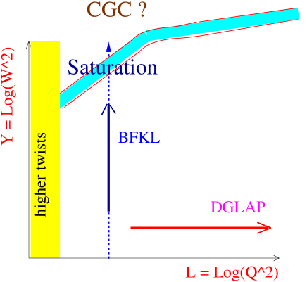
Figure 1: Schematic view of the transition region to saturation. The DGLAP and BFKL evolution ranges are displayed, together with the saturation region where the density bounds are reached.

The problem we address here is the characterization of the gluon-momentum distribution near saturation. Our aim is to understand the transverse-momenta spectrum of the gluons which are generated by the BFKL evolution in rapidity, i.e. as characterising a transient QCD phase structure near saturation as a whole. The new material contained in this lecture comes from Ref. RP .

As a guide for the further developments, the basic structure underlying the transition to saturation can be understood in terms of traveling waves. If at first one neglects the fluctuations (in the mean-field approximation), the effect of saturation on a dipole-target amplitude is described by the nonlinear Balitsky-Kovchegov Balitsky (BK) equation, where a nonlinear damping term adds to the BFKL equation. As shown in munier , this equation falls into the universality class of the Fisher and Kolmogorov Petrovsky Piscounov (F-KPP) nonlinear equation KPP which admits asymptotic traveling-wave solutions. The exponential behaviour of the BFKL evolution quickly enhances the effects of the tail towards a region where finally the nonlinear damping regulates both the traveling-wave propagation and structure.

Indeed, one of the major recent challenges in QCD saturation is the problem of taking into account the rôle of fluctuations, i.e. the structure of gluon momenta beyond the average. In these conditions it was realized for traveling waves brunet and thus in the QCD case Iancu:2004es , that the fluctuations may have a surprisingly large effect on the overall solution of the nonlinear equations of saturation. Indeed, a fluctuation in the dilute regime may grow exponentially and thus modify its contribution to the overall amplitude. Hence, in order to enlarge our understanding of the QCD evolution with rapidity, it seems important to give a quantitative description of the pattern of momenta generated by the BFKL evolution equations for the set of cascading dipoles (or, equivalently gluons) near saturation, which is the subject of the lecture.

Technically speaking, we shall work in the leading order in $1/N_{c},$ where the QCD dipole framework is valid Mueller:1993rr . Moreover we will use the diffusive approximation of the 1-dimensional BFKL kernel. In fact, the phase structure appears quite rich already within this approximation scheme. Many aspects we will obtain show “universality” features and thus are expected to be valid beyond the approximations.

IV.2 Rapidity evolution of cascading QCD dipoles

2.  Let us start by briefly describing the QCD evolution of the dipole distributions Mueller:1993rr ; salam ; Hatta:2006hs .

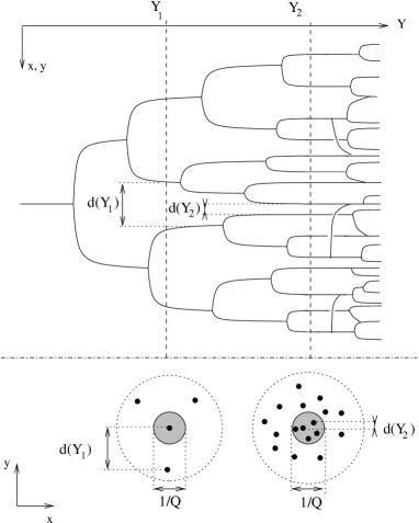
Figure 2: BFKL cascading and saturation. The QCD branching process in the BFKL regime and beyond is represented along the rapidity axis (upper part). Its 2-dimensional counterpart in transverse position space is displayed at two different rapidities (lower part). The interaction region is represented by a shaded disk of size $1/Q$. At rapidity $Y_{1}$, the interaction still probes individual dipoles (or gluons), which corresponds to the exponential BFKL regime. There exists a smooth transition to a regime where the interaction only probes groups of dipoles or gluons, e.g. at rapidity $Y_{2}$. This gives a description of the near-saturation region corresponding to a mean-field approximation, where correlations can be neglected. Further in rapidity, $Y>Y_{2},$ other dynamical effects, such that merging and correlations appear.

The structure of BFKL cascading describes a 2-dimensional tree structure of dipoles in transverse position space evolving with rapidity. Let us, for instance, focus on the rapidity evolution starting from one massive $q\bar{q}$ pair or onium Mueller:1993rr , see Fig.2. At each branching vertex, the wave function of the onium-projectile is described by a collection of color dipoles. The dipoles split with a probability per unit of rapidity defined by the BFKL kernel bfkl

$${\cal K}({\bf v},{\bf w};{\bf z})={\alpha_{s}N_{c}}/{\pi}\ \frac{\left({\bf v}-{\bf w}\right)^{2}}{\left({\bf v}-{\bf z}\right)^{2}\left({\bf z}-{\bf w}\right)^{2}}\$$ (1)

describing the dissociation vertex of one dipole $({\bf v},{\bf w})$ into two dipoles at $({\bf v},{\bf z})$ and $({\bf z},{\bf w}),$ where ${\bf v},{\bf w},{\bf z}$ are arbitrary 2-dimensional transverse space coordinates.

As an approximation of the 2-dimensional formulation of the BFKL kernel (1) obtained when one neglects the impact-parameter dependence, we shall restrict our analysis in the present paper to the 1-dimensional reduction of the problem to the transverse-momenta moduli $k_{i}$ of the cascading gluons. After Fourier transforming to transverse-momentum space, the leading-order BFKL kernel bfkl defining the rapidity evolution in the 1-dimensional approximation is known Balitsky to act in transverse momentum space as a differential operator of infinite order

$$\chi(-\partial_{l})\equiv 2\psi(1)-\psi(-\partial_{l})-\psi(1+\partial_{l})$$ (2)

where $l=\log k^{2}$ and $Y$ is the rapidity in units of the fixed coupling constant ${\alpha_{s}N_{c}}/{\pi}$.

In the sequel, we shall restrict further our analysis to the diffusive approximation of the BFKL kernel. We thus expand the BFKL kernel to second order around some value $\gamma_{c}$

$$\chi(\gamma)\sim\chi_{c}+\chi^{\prime}_{c}(\gamma-\gamma_{c})+{\scriptstyle\frac{1}{2}}\chi^{\prime\prime}_{c}(\gamma-\gamma_{c})^{2}=A_{0}-A_{1}\gamma+A_{2}\gamma^{2}\ ,$$ (3)

where $\gamma_{c}$ will be defined in such a way to be relevant for the near-saturation region of the BFKL regime.

Within this diffusive approximation, it is easy to realize that the first term ($A_{0}$) is responsible for the exponential increase of the BFKL regime while the third term ($A_{2}$) is a typical diffusion term. The second term ($A_{1}$) is a “shift” term since it amounts to a rapidity-dependent redefinition of the kinematic variables, as we shall see.

In Eq.(3), $\gamma_{c}$ is chosen in order to ensure the validity of the kernel (3) in the transition region from the BFKL regime towards saturation. Indeed, the derivation of asymptotic solutions of the BK equation munier leads to consider the condition

$$\chi(\gamma_{c})=\gamma_{c}\ \chi^{\prime}(\gamma_{c})\$$ (4)

whose solution determines $\gamma_{c}.$

This condition applied to the kernel formula (2) gives $\gamma_{c}=\sqrt{A_{0}/A_{2}}\approx 0.6275...$ and $\{A_{0},A_{1},A_{2}\}\approx\{9.55,25.56,24.26\}.$ These numbers may appear anecdotic, but they fully characterize the critical parameters of the saturation transition, as we will realize later on. For different kernels, e.g. including next-leading log effects Peschanski:2005ic , they could be different, of course. But, then the traveling-wave solution will be in a different “universality class” in mathematical terms.

IV.3 Mapping to thermodynamics of directed polymers

3. From the properties in transverse-momentum space and within the 1-dimensional diffusive approximation (3), we already noticed that the BFKL kernel models boils down to a branching, shift and diffusion operator acting in the gluon transverse-momentum-squared space. Hence the cascade of gluons can be put in correspondence with a continuous branching, velocity-shift and diffusion probabilistic process, see Fig.2, whose probability by unit of rapidity is defined by the coefficients $A_{i}$ of (3).

Figure 3: Branching diffusion model for polymers. The coordinates $x_{1}(t)\cdots x_{7}(t)$ correspond to the random paths along the tree in the $x,t$ phase-space. The oblique axis is for $L=\beta x+{A_{1}}/{A_{0}}\ t,$ which takes into account the “time-drift” in the mapping to the QCD problem.

Let us first introduce the notion of gluon-momenta “histories” $k_{i}(y).$ They register the evolution of the gluon-momenta starting from the unique initial gluon momentum $k(0)$ and terminating with the specific $i$-th momentum $k_{i},$ after successive branchings. They define a random function of the running rapidity $y,$ with $0\leq y\leq Y,$ the final rapidity range when the evolution ends up (say, for a given total energy). It is obvious that two different histories $k_{i}(y)$ and $k_{j}(y)$ are equal before the rapidity when they branch away from their common ancestor.

In order to fromulate precisely the mapping to the polymer problem, we then introduce random paths $x_{i}(t)$ using formal space and time coordinates $x,t\ ,\ 0\leq t\leq{\Delta t}$ which we relate to gluon-momenta “histories” as follows:

$$\ y=\ \frac{t}{A_{0}}\ ;\quad\quad\log{k_{i}^{2}(y)}\equiv-\beta\ (x_{i}(t)-x(0))+({A_{0}}-{A_{1}})y$$ (5)

where $(A_{0}-A_{1})y$ is a conveniently chosen and deterministic “drift term”, $x(0)$ is an arbitrarily fixed origin of an unique initial gluon and thus the same for all subsequent random paths. The random paths $x_{i}(t)$ are generated by a continuous branching and Brownian diffusion process in space-time (cf. Fig.3).

As we shall determine later on, the important parameter $\beta,$ which plays the rôle of an inverse of the temperature $T$ for the Brownian movements of the polymer process, is given by

$$\frac{1}{T}\equiv\beta=\sqrt{{2A_{2}}/{A_{0}}}\ .$$ (6)

In fact, the relation (6) will be required by the condition that the stochastic process of random paths describes the BFKL regime of QCD near saturation. Another choice of $\beta$ would eventually describe the same branching process but in other conditions. Hence the condition (6) will be crucial to determine the QCD phase at saturation (within the diffusive approximation).

Let now introduce the tree-by-tree random function defined as the partition function of the random paths system

$$Z(t)\equiv\sum_{i=1}^{n}e^{-\beta x_{i}(t)}=e^{-\beta x_{0}+A_{1}y}\times\frac{1}{n}\sum_{i=1}^{n=e^{A_{0}y}}k_{i}^{2}(y)\ \propto\ e^{A_{1}y}\times\bar{k}^{2}(y)\ ,$$ (7)

where $\frac{1}{n}\sum_{i=1}^{n}k_{i}^{2}(y)\equiv\bar{k}^{2}(y)$ is the event-by-event average over gluon momenta at rapidity $y.$ Note that one has to distinguish $\ \overline{\ \cdots\ }$ i.e. the average made over only one event from $\langle\ \cdots\ \rangle,$ which denotes the average over samples (or events).

$Z(t)$ is an event-by-event random function. The physical properties are obtained by averaging various observables over the events. Note that the distinction between averaging over one event and the sample-to-sample averaging appears naturally in the statistical physics problem in terms of “quenched” disorder: the time scale associated with the averaging over one random tree structure is much shorter than the one corresponding to the averaging over random trees.

With these definitions, $Z$ appears to be nothing else than the partition function for the model of directed polymers on a random tree Derrida .

Let us now justify the connection of the directed-polymer properties with the description of the gluon-momentum phase near saturation by rederiving the known saturation features from the statistical model point-of-view. Using the known properties Derrida of the partition function of the polymer problem, one finds

$$\log Q_{s}^{2}\equiv\langle\ \log\bar{k}^{2}\ \rangle\equiv\langle\ \log Z\ \rangle-A_{1}Y=\left[(2\sqrt{{A_{2}}{A_{0}}}-A_{1})Y-\frac{3}{2}\sqrt{\frac{A_{0}}{A_{2}}}\log Y\right]+{\cal O}(1)\ ,$$ (8)

which in fact matches exactly the asymptotic expansion found in munier for the saturation scale.

In the same way, the solution of the statistical-physics problem allows to derive the event-by-event spectrum of the free energy $\log Z(t)$ of the system around its average. From (7), one gets

$${\cal N}(\bar{k}^{2},Y)\sim{\cal P}\left(\log Z-\langle\log Z\rangle\right)\ \propto\ \log\left[\frac{\bar{k}^{2}}{Q_{s}^{2}}\right]\ \exp\left\{-\sqrt{\frac{A_{0}}{A_{2}}}\log\left[\frac{\bar{k}^{2}}{Q_{s}^{2}}\right]\right\}\ ,$$ (9)

which is the well-known geometrical scaling property, empirically found in Ref.geom and theoretically derived in munier from the BK equation for the dipole amplitude ${\cal N}(\bar{k}^{2},Y).$

Both properties (8),(9) prove the consistency of the model with the properties expected from saturation. We shall then look for other properties of the cascading gluon model. It is important to realize that this consistency fails for a different choice of the parameter $\beta$ different from (6). This justifies a-posteriori the identification of the equivalent temperature of the system in the gluon/polymer mapping framework.

IV.4 The Spin-Glass Phase of gluons

4. Let us now come to the main new results concerning the determination of structure of the gluon-momentum phase at saturation.

The striking property of the directed polymer problem on a random tree is the spin-glass structure of the low temperature phase. As we shall see this will translate directly into a specific clustering structure of gluon transverse momenta in their phase near the “unitarity limit”, see Fig.4.

Figure 4: The clustering structure of gluons near saturation. The drawing represents the $s_{1}\cdots s_{4}$ clusters near momenta $k_{s1}\cdots k_{s4}$. They branch either near $t\ll 1$ or $(\Delta t-t)\ll 1,$ where $\Delta t$ is the total amount of time evolution.

Following the relation (6) , one is led to consider the polymer system at temperature $T$ with

$$\frac{T_{c}-T}{T_{c}}\equiv 1-\frac{\beta_{c}}{\beta}=1-\gamma_{c}\ ,$$ (10)

where $\gamma_{c}$ is the critical exponent defined by (4). We are thus naturally led to consider the low-temperature phase ($T<T_{c}$), at some distance $T_{c}-T$ from the critical temperature $T_{c}=\scriptstyle{1/{\sqrt{2}}}.$ In the language of traveling waves wave , this corresponds to a “pulled-front” condition with “frozen”and “universal” velocity and front profile.

As derived in Derrida , the phase space of the polymer problem is structured in “valleys” which are in the same universality class as those of the Random Energy Model (REM) REM and of the infinite range Sherrington-Kirkpatrick (SK) model SK .

Translating these results in terms of gluon-momenta moduli, the phase space landscape consists in event-by-event distribution of clusters of momenta around some values $k_{si}^{2}\equiv 1/(n_{i})\ \sum_{i\in si}k_{i}^{2},$ where $n_{i}$ is the cluster multiplicity. The probability weights to find a cluster $s_{i}$ after the whole evolution range $Y$ is defined by

$$W_{si}=\frac{\sum_{i\in si}k_{i}^{2}}{\sum_{i}k_{i}^{2}},$$ (11)

where the summation in the numerator is over the momenta of gluons within the $s_{i}^{th}$ cluster (see Fig.4). The normalized distribution of weights $W_{si}$ thus allows one to study the probability distribution of clusters. The clustering tree structure, (called “ultrametric” in statistical mechanics) is the most prominent feature of spin-glass systems overlap .

Note again that, for the QCD problem, this property is proved for momenta in the region of the “unitarity limit”, or more concretely in the momentum region around the saturation scale. This means that the cluster average-momentum is also such that $k_{si}^{2}={\cal O}(Q^{2}_{s}).$ Hence the clustering structure is expected to appear in the range which belongs to the traveling-wave front munier or, equivalently, of clustering with finite fluctuations around the saturation scale.

In order to quantify the cluster structure, one may introduce a well-known “overlap function” in statistical physics of spin-glasses overlap . Translating the definitions (cf. Derrida ) in terms of the QCD problem, one introduces an event-by-event indicator of the strength of clustering which is built in from the weights (11), namely ${\cal Y}=\sum_{si}W^{2}_{si}.$ The non-trivial probability distribution of overlaps ${\Pi}({\cal Y})$ possesses some universality features, since it is identical to the one of the REM and SK models and shares many qualitative similarities with other systems possessing a spin-glass phase toulouse ; toulouse1 . Exemples are given in Fig.5.

Figure 5: The probability distribution of overlaps ${\Pi}({\cal Y})$. The figure (the simulation is by courtesy from private , using the method of Ref.toulouse1 ) is drawn both for the theoretical QCD value $\gamma_{c}=0.7,$ and for $\gamma_{c}=0.3$ for comparison. The statistics used for the simulation is $10^{8}$ events in $10^{3}$ bins for $\gamma_{c}=0.3$ and $3.25\ 10^{6}$ events in $10^{2}$ bins for $\gamma_{c}=0.7.$

The rather involved probability distribution $\Pi({\cal Y})$ is quite intringuing. It possesses a priori an infinite number of singularities at ${\cal Y}=1/n,n\ {\rm integer}.$ It can be seen when the temperature is significantly lower from the critical value, see for instance the curve for $1-T/T_{c}=.7$ in Fig.5. However, the predicted curve for the QCD value $1-T/T_{c}\sim.3$ is smoother and shows only a final cusp at $W_{s}=1$ within the considered statistics. It thus seems that configurations with only one cluster can be more prominent than the otherwise smooth generic landscape. However, it is also a “fuzzy” landscape since many clusters of various sizes seem to coexist in general.

IV.5 Summary of lecture I

5. We investigated the landscape of transverse momenta in gluon cascading around the saturation scale at asymptotic rapidity. Limiting our study to a diffusive 1-dimensional modelization of the BFKL regime of gluon cascading, we make use of a mapping on a statistical physics model for directed polymers propagating along random tree structures at fixed temperature. We then focus our study on the region near the unitarity limit where information can be obtained on saturation, at least in the mean-field approximation. Our main result is to find a low-temperature spin-glass structure of phase space, characterized by event-by-event clustering of gluon transverse momenta (in modulus) in the vicinity of the rapidity-dependent saturation scale. The weight distribution of clusters and the probability of momenta overlap during the rapidity evolution are derived.

Interestingly enough the clusters at asymptotic rapidity are branching either near the beginning (“overlap $0$” or $y/Y\ll 1$) or near the end (“overlap $1$” or $1-y/Y\ll 1$) of the cascading event. The probability distribution of overlaps is derived and shows a rich singularity structure.

On a phenomenological ground, it is remarkable that saturation density effects are not equally spread out on the event-by-event set of gluons; our study suggests that there exists random spots of higher density whose distribution may possess some universality properties. In fact it is natural to expect this clustering property to be present not only in momentum modulus (as we could demonstrate) but also in momentum azimuth-angle. This is reminiscent of the “hot spots” which were some time ago Bartels:1992bx advocated from the production of forward jets in deep-inelastic scattering at high energy (small-$x$). The observability of the cluster distribution through the properties of “hot spots” is an interesting possibility.

V Lecture II: A Perfect Fluid from Gauge/Gravity Duality

V.1 Introduction

6. From the first years of the running of heavy-ion collisions at RHIC, evidence has been advocated that various observables are in good agreement with models based on hydrodynamics hydro and with quark-gluon plasma (QGP) in a strongly coupled regime strongQGP . To a large extent it seems that the QGP behaves approximately as a perfect fluid as was first considered in Bjorken . A schematic view of the theoretical expectations in given in Fig.6. It is a challenge in QCD to derive from first principles the properties of the dynamics of a strongly interacting plasma formed in heavy-ion collisions and in particular to understand why the perfect-fluid hydrodynamic equations appear to be relevant.

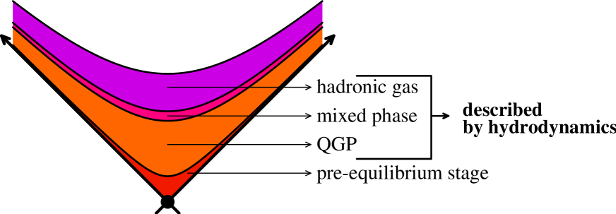
Figure 6: Scenario for the quark-gluon plasma(QGP) formation. After a pre-equilibrium stage in a heavy-ion collision, probably governed by a weak-coupling but dense regime, the QGP is formed with local equilibrium and hydrodynamic properties.

Even if the experimental situation is still developing and rather complex, it is worth simplifying the problem in order to be able to attack it with appropriate theoretical tools. Recently the AdS/CFT correspondence adscft ; adscftrev emerged as a new approach to study strongly coupled gauge theories. This has been largely worked out in the supersymmetric case and in particular for the conformal case of ${\cal N}=4$ super Yang-Mills theory (SYM). Interestingly enough, since the QGP is a deconfined and strongly interacting phase of QCD we could expect that results for the nonconfining ${\cal N}=4$ theory may be relevant or at least informative on the unknown strong coupling QCD problem. We will start from this assumption in our work.

In this lecture we focus on the spacetime evolution of the gauge theory (4d) energy-momentum tensor, and derive its asymptotic behaviour from the solutions of the nonlinear Einstein equations of the gravity dual.

Imposing the absence of curvature singularities in the gravity dual, we will show that, in the boost invariant setting (as in Bjorken ), perfect fluid hydrodynamics emerges from the AdS/CFT solution at large times. The new material contained here comes from Refs. janik .

V.2 String/Gauge fields Duality

7. As an introduction to our lecture, let us briefly recall some aspects of the String/Gauge Duality. The AdS/CFT correspondence adscft has many interesting formal and physical facets. Concerning the aspects which are of interest for our problem, it allows one to find relations between gauge field theories at strong coupling and string gravity at weak coupling in the limit of large number of colours ($N_{c}\!\to\!\infty$). It can be examined quite precisely in the AdS₅/CFT₄ case which conformal field theory corresponds to $SU(N)$ gauge theory with ${\cal N}\!=\!4$ supersymmetries.

Let us recall the canonical derivation leading to the AdS₅ background , see Fig.7. One starts from the (super)gravity classical solution of a system of $N\ D_{3}$-branes in a $10\!-\!D$ space of the (type IIB) superstrings. The metrics solution of the (super)Einstein equations read

$$ds^{2}=f^{\!-\!1/2}(\!-\!dt^{2}\!+\!\sum_{1\!-\!3}dx_{i}^{2})\!+\!f^{1/2}(dr^{2}\!+\!r^{2}d\Omega_{5})\ ,$$ (12)

where the first four coordinates are on the brane and $r$ corresponds to the coordinate along the normal to the branes. In formula (12), one defines

$$f=1+\frac{R^{4}}{r^{4}}\ ;\ \ \ \ \ R=4\pi g^{2}_{YM}\alpha^{\prime 2}{N}\ ,$$ (13)

where $g^{2}_{YM}{N}$ is the ‘t Hooft-Yang-Mills coupling and $\alpha^{\prime}$ the string tension.

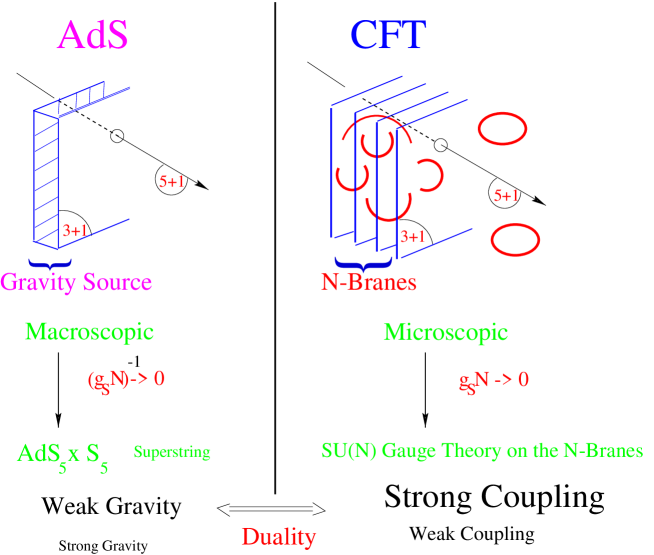
Figure 7: Schematic view of the Gauge/String Duality. Left: The string background is the Anti-de Sitter space (AdS); Right: the gauge theory is a Conformal field theory (CFT) on the 4-d N-branes.

One considers the limiting behaviour considered by Maldacena, where one zooms on the neighbourhood of the branes while in the same time going to the limit of weak string slope $\alpha^{\prime}.$ The near-by space-time is thus distorted due to the (super) gravitational field of the branes. One goes to the limit where

$$\ R\ fixed\ ;\ \frac{\alpha^{\prime}(\to 0)}{r(\to 0)}\to z\ fixed\ .$$ (14)

This, from the second equation of (13) obviously implies

$${\alpha^{\prime}\to 0}\ ,\ g^{2}_{YM}{N}\sim\frac{1}{\alpha^{\prime 2}}\to\infty\ ,$$ (15)

i.e. both a weak coupling limit for the string theory and a strong coupling limit for the dual gauge field theory. By reorganizing the two parts of the metrics one obtains

$$ds^{2}={\frac{1}{z^{2}}(-dt^{2}+\sum_{1-3}dx_{i}^{2}+dz^{2})}+{R^{2}d\Omega_{5}}\ ,$$ (16)

which corresponds to the AdS₅ $\times\ {S_{5}}$ background structure, ${S_{5}}$ being the 5-sphere. More detailed analysis shows that the isometry group of the 5-sphere is the geometrical dual of the ${\cal N}\!=\!4$ supersymmetries. More intricate is the quantum number dual to $N_{c},$ the number of colours, which is the invariant charge carried by the Ramond-Ramond form field.

V.3 Bjorken hydrodynamics

8. Coming back to the physical world, a model of the central rapidity region of heavy-ion reactions based on hydrodynamics was pioneered in Bjorken and involved the assumption of boost invariance. Our goal is to study the dynamics of strongly interacting gauge-theory matter assuming boost invariance.

We will be interested in the spacetime evolution of the energy-momentum tensor $T_{\mu\nu}$ of the gauge-theory matter. It is convenient to introduce proper-time ($\tau$) and space-rapidity ($y$) coordinates in the longitudinal position plane:

$$x^{0}=\tau\cosh y\quad\quad\quad\quad x^{1}=\tau\sinh y\ .$$ (17)

In these coordinates, all components of the energy momentum tensor can be expressed (see janik ) in terms of a single function $f(\tau)$:

$$T_{\mu\nu}\!=\!\left(\begin{tabular}[]{cccc}$f(\tau)$&0&0&0\\ 0&$-\tau^{3}\frac{d}{d\tau}f(\tau)\!-\!\tau^{2}f(\tau)$&0&0\\ 0&0&$f(\tau)\!+\!\frac{1}{2}\tau\frac{d}{d\tau}f(\tau)$&0\\ 0&0&0&$f(\tau)\!+\!\frac{1}{2}\tau\frac{d}{d\tau}f(\tau)$\end{tabular}\right)$$ (18)

where the matrix $T_{\mu\nu}$ is expressed in $(\tau,y,x_{1},x_{2})$ coordinates.

Furthermore the function $f(\tau)$ is constrained to verify

$$f(\tau)\geq 0\quad\quad\quad\quad f^{\prime}(\tau)\leq 0\quad\quad\quad\quad\tau f^{\prime}(\tau)\geq-4f(\tau)\ .$$ (19)

The dynamics of the gauge theory should pick a specific $f(\tau)$. A perfect fluid or a fluid with nonzero viscosity and/or other transport coefficients will lead to different choices of $f(\tau)$.

We thus address the problem of determination of the function $f(\tau)$ from the AdS/CFT correspondence. Let us first describe two distinct cases of physical interest:

For a perfect fluid (Bjorken hydrodynamics) $f(\tau)\sim{1}/{\tau^{\frac{4}{3}}},$ while for a “free streaming case” expected just at the beginning of the interaction Kovchegov , $f(\tau)\sim{1}/{\tau}.$ In the following we introduce a family of $f(\tau)$ with the large $\tau$ behaviour of the form

$$f(\tau)\sim\tau^{-s}.$$ (20)

V.4 Boost-invariant geometries

9. The most general form of the bulk metric respecting boost-invariance can be written

$$ds^{2}=\frac{-e^{a(\tau,z)}d\tau^{2}+\tau^{2}e^{b(\tau,z)}dy^{2}+e^{c(\tau,z)}dx^{2}_{\perp}}{z^{2}}+\frac{dz^{2}}{z^{2}}\ .$$ (21)

The three coefficient functions can be (non trivially) derived from the Einstein equations

$$R_{\mu\nu}-\frac{1}{2}g_{\mu\nu}R-6\,g_{\mu\nu}=0\ ,$$ (22)

in the asymptotic limit where $\tau\to\infty.$ Interestingly enough, they depend only on the scaling variable $v=z/\tau^{s/4},$ where $s$ labels the one-parameter family of solutions (20).

After quite painful calculations, the solution reads janik

$$a(v)=A(v)-2m(v)\ b(v)=A(v)+(2s-2)m(v)\ c(v)=A(v)+(2-s)m(v)$$ (23)

where

$$A(v)=\frac{1}{2}\left(\log(1+\Delta(s)\,v^{4})+\log(1-\Delta(s)\,v^{4})\right)\ m(v)=\frac{1}{4\Delta(s)}\left(\log(1+\Delta(s)\,v^{4})-\log(1-\Delta(s)\,v^{4})\right)$$ (24)

with

$$\Delta(s)=\sqrt{\frac{3s^{2}-8s+8}{24}}\ .$$ (25)

Specializing first to the perfect fluid case, this gives rise to the following asymptotic geometry

$$z^{2}\ ds^{2}=-\frac{\left(1-\frac{e_{0}}{3}\frac{z^{4}}{\tau^{4/3}}\right)^{2}}{1+\frac{e_{0}}{3}\frac{z^{4}}{\tau^{4/3}}}d\tau^{2}+\left({\textstyle 1+\frac{e_{0}}{3}\frac{z^{4}}{\tau^{4/3}}}\right)(\tau^{2}dy^{2}+dx^{2}_{\perp})+{dz^{2}}$$ (26)

Remarkably enough this geometry can be identified (in suitable metrics) to be a moving Black Hole, which evolves in the fifth dimension $z.$

For the free streaming case, one finds

$$z^{2}\ ds^{2}={-(1\!+\!\frac{v^{4}}{\sqrt{8}})^{\frac{1\!-\!2\sqrt{2}}{2}}(1\!-\!\frac{v^{4}}{\sqrt{8}})^{\frac{1\!+\!2\sqrt{2}}{2}}dt^{2}+(1\!+\!\frac{v^{4}}{\sqrt{8}})^{\frac{1}{2}}(1\!-\!\frac{v^{4}}{\sqrt{8}})^{\frac{1}{2}}\tau^{2}dy^{2}+(1\!+\!\frac{v^{4}}{\sqrt{8}})^{\frac{1\!+\!\sqrt{2}}{2}}(1\!-\!\frac{v^{4}}{\sqrt{8}})^{\frac{1\!-\!\sqrt{2}}{2}}dx^{2}_{\perp}}+{dz^{2}}\ ,$$ (27)

which is qualitatively different from the perfect fluid case, in particular it displays singularities or zeroes at $v^{4}=\sqrt{8}$ in all coefficients. More generally, it is possible to show janik that the perfect fluid case is the only one free of physical singularities, namely singularities which cannot be removed by a change of coordinates. In order to check this feature, we considered the metric-invariant curvature scalar

$${\mathfrak{R}^{2}}=R^{\mu\nu\alpha\beta}R_{\mu\nu\alpha\beta}\ .$$ (28)

As an illustration, we represent this property in Fig.8, where the value of ${\mathfrak{R}^{2}}$ is studied as a function of the distance from the horizon, for $s$ values at the perfect fluid point and very near-by values.

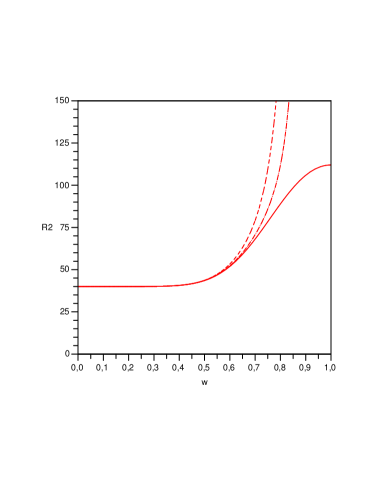
Figure 8: The curvature scalar ${\mathfrak{R}^{2}}.$ ${\mathfrak{R}^{2}}$ is calculated as a function of $w=v/\Delta(s)^{1/4}$ for the perfect fluid case $s=4/3$ (solid line), $s=4/3-0.1$ (dotted line) and $s=4/3+0.2$ (dashed line).

Let us add some comments on the specific features of our approach and results. We concentrate on looking for solutions of the full nonlinear Einstein equations. It would be interesting to confront this approach with the linearization methods of refs. son . In particular viscosity terms are expected to appear in the study of subasymptotic terms. Note that the possibility of black hole formation in the dual geometry has been argued in ref. nastase . More specifically, the geometry of a brane moving w.r.t. a black hole background has been advocated in ref. zahedsin for the dual description of the cooling and expansion of a quark-gluon plasma. In our case we could interpret the solution (26) as a kind of ‘mirror’ situation in terms of a black hole moving off from the AdS boundary.

V.5 Summary of Lecture II

10.  We have introduced a general framework for studying the dynamics of matter (plasma) in strongly coupled gauge theory using the AdS/CFT correspondence for the ${\cal N}=4$ SYM theory. We constructed dual geometries for given 4-dimensional gauge theory energy-momentum tensor profiles. Further imposing boost-invariant dynamics inspired by the Bjorken hydrodynamic picture, we have found the corresponding asymptotic solutions of the nonlinear Einstein equations. Among the family of asymptotic solutions, the only one with bounded curvature scalars is the gravity dual of a perfect fluid through its energy-momentum tensor profile. This selected nonsingular solution, given by the metric (26), corresponds to a black hole moving off in the 5th dimension as a function of the physical proper time. As an application of this framework, we can obtain janik the thermalization time of the perfect fluid, which describes the decay back to equilibrium of a scalar excitation of the perfect fluid out of equilibrium, by computation of the quasi-normal modes of the moving Black Hole. In some sense, the moving Black Hole is a quite stable geometric configuration. We conjecture that it may represent, through the Gauge/Gravity duality, a powerful “attractor” for the QGP evolution, or even perhaps for more general evolution of a strongly coupled system of quarks and gluons.

Acknowledgments. Many aspects depicted in Lecture I come from constant collaboration and discussion inside (and outside) our “Saturation Team” in Saclay 2006, in particular Edmond Iancu, Cyrille Marquet, Gregory Soyez. I warmly thank Romuald Janik for its major contribution in the fruitful collaboration whose results are discussed in Lecture II.

References

- (1) L. N. Lipatov, Sov. J. Nucl. Phys. 23, 338 (1976); E. A. Kuraev, L. N. Lipatov, and V. S. Fadin, Sov. Phys. JETP 45, 199 (1977); I. I. Balitsky and L. N. Lipatov, Sov. J. Nucl. Phys. 28, 822 (1978).
- (2) G.Altarelli and G.Parisi, Nucl. Phys. B126 18C (1977) 298. V.N.Gribov and L.N.Lipatov, Sov. Journ. Nucl. Phys. (1972) 438 and 675. Yu.L.Dokshitzer, Sov. Phys. JETP. 46 (1977) 641.
- (3) L.V. Gribov, E.M. Levin and M.G. Ryskin, Phys. Rep. 100, 1 (1983).
- (4) L. McLerran and R. Venugopalan, Phys. Rev. D 49, 2233 (1994); 49, 3352 (1994); 50, 2225 (1994); A. Kovner, L. McLerran and H. Weigert, ibid. 52, 6231 (1995); 52, 3809 (1995); R. Venugopalan, Acta Phys.Pol. B 30, 3731 (1999); E. Iancu, A. Leonidov, and L. McLerran, Nucl. Phys. A692, 583 (2001); idem, Phys. Lett. B 510, 133 (2001); E. Iancu and L. McLerran, ibid. 510, 145 (2001); E. Ferreiro, E. Iancu, A. Leonidov and L. McLerran, Nucl. Phys. A703, 489 (2002); H. Weigert, ibid. A703, 823 (2002). For comprehensive reviews on saturation and other references, see e.g. A.H. Mueller, “Parton saturation: An overview”, hep-ph/0111244; E. Iancu and R. Venugopalan, “The color glass condensate and high energy scattering in QCD,” arXiv:hep-ph/0303204.
- (5) R. Peschanski, Nucl. Phys. B 744, 80 (2006) [arXiv:hep-ph/0602095].
- (6) I. I. Balitsky, Nucl. Phys. B 463, 99 (1996) [arXiv:hep-ph/9509348]; Y. V. Kovchegov, Phys. Rev. D60, 034008 (1999), [arXiv:hep-ph/9901281].
- (7) S. Munier and R. Peschanski, Phys. Rev. Lett. 91, 232001 (2003) [arXiv:hep-ph/0309177]; Phys. Rev. D69, 034008 (2004) [arXiv:hep-ph/0310357]; Phys. Rev. D70, 077503 (2004) [arXiv:hep-ph/0310357].
- (8) R. A. Fisher, Ann. Eugenics 7, 355 (1937); A. Kolmogorov, I. Petrovsky, and N. Piscounov, Moscou Univ. Bull. Math. A1, 1 (1937).
- (9) E. Brunet and B. Derrida, Phys. Rev. E57 (1997) 2597 [arXiv:cond-mat/0005362]; Comp. Phys. Comm. 121 (1999) 376 [arXix:cond-mat/0005364].
- (10) A. H. Mueller and A. I. Shoshi, Nucl. Phys. B 692 (2004) 175 [arXiv:hep-ph/0402193]; E. Iancu, A. H. Mueller and S. Munier, Phys. Lett. B 606, 342 (2005) [arXiv:hep-ph/0410018]. S. Munier, Nucl. Phys. A 755, 622 (2005) [arXiv:hep-ph/0501149]; E. Iancu and D. N. Triantafyllopoulos, Nucl. Phys. A 756 (2005) 419 [arXiv:hep-ph/0411405]; Phys. Lett. B 610 (2005) 253 [arXiv:hep-ph/0501193]. C. Marquet, R. Peschanski and G. Soyez, Phys. Rev. D 73, 114005 (2006) [arXiv:hep-ph/0512186].
- (11) A. H. Mueller, Nucl. Phys. B 415, 373 (1994); A. H. Mueller and B. Patel, Nucl. Phys. B 425, 471 (1994) [arXiv:hep-ph/9403256]; A. H. Mueller, Nucl. Phys. B 437, 107 (1995) [arXiv:hep-ph/9408245]. See also, N. N. Nikolaev and B. G. Zakharov, Z. Phys. C49 (1991) 607.
- (12) G. P. Salam, Nucl. Phys. B 449, 589 (1995) [arXiv:hep-ph/9504284], ibid. 461, 512 (1996) [arXiv:hep-ph/9509353]; Comput. Phys. Commun. 105, 62 (1997) [arXiv:hep-ph/9601220]; A. H. Mueller and G. P. Salam, Nucl. Phys. B 475, 293 (1996) [arXiv:hep-ph/9605302].
- (13) For recent discussion and applications of the dipole generating functionale, see Y. Hatta, E. Iancu, C. Marquet, G. Soyez and D. N. Triantafyllopoulos, Nucl. Phys. A 773, 95 (2006) [arXiv:hep-ph/0601150]
- (14) R. Peschanski, Phys. Lett. B 622, 178 (2005) [arXiv:hep-ph/0505237]; C. Marquet, R. Peschanski and G. Soyez, Phys. Lett. B 628, 239 (2005) [arXiv:hep-ph/0509074].
- (15) B. Derrida and H. Spohn, J. Stat. Phys. 51, 817 (1988).
- (16) M. Bramson, Mem. Am. Math. Soc. 44, 285 (1983); E. Brunet and B. Derrida, Phys. Rev. E56, 2597 (1997); U. Ebert, W. van Saarloos, Physica D 146, 1 (2000).
- (17) A. M. Staśto, K. Golec-Biernat, and J. Kwiecinski, Phys. Rev. Lett. 86, 596 (2001), [arXiv:hep-ph/0007192].
- (18) G. Soyez, private communication.
- (19) B. Derrida, Phys. Rev. Lett. 45, 79 (1980) Phys. Rev. B 24,2613 (1980)
- (20) D. Sherrington and S. Kirkpatrick Phys. Rev. Lett. 35, 1972 (1975) Phys. Rev. B 17, 4384 (1978)
- (21) The classical book on spin-glass theory and the overlap function is: M. Mézard, G. Parisi and M. A. Virasoro “Spin glass theory and beyond” World Scientific Lecture Notes in Physics, 9 (1987).
- (22) B. Derrida and G. Toulouse J. Physique Lett. 46, L223 (1985);
- (23) B. Derrida and H. Flyvbjerg J. Phys. A: Math. Gen. 20, 5273 (1987).
- (24) A. H. Mueller, Nucl. Phys. Proc. Suppl. B18C (1990) 125; J. Phys. G17 (1991) 1443. Jochen Bartels (Hamburg U.), M. Besancon (Saclay), A. De Roeck (Munich, Max Planck Inst.), J. Kurzhofer (Dortmund U.),. 1991, “Measurement of hot spots at HERA, In *Hamburg 1991, Proceedings, Physics at HERA, vol. 1* 203-213. (see High energy physics index 30 (1992) No. 12988). J. Bartels, “Measurement of hot spots in the proton at HERA,” Prepared for International Workshop on Quark Cluster Dynamics, Bad Honnef, Germany, 29 Jun - 1 Jul 1992 J. Bartels and H. Lotter, Phys. Lett. B 309, 400 (1993).
- (25) P. F. Kolb and U. W. Heinz, “Hydrodynamic description of ultrarelativistic heavy-ion collisions,” arXiv:nucl-th/0305084.
- (26) see e.g. E. V. Shuryak, Nucl. Phys. A 750 (2005) 64 [arXiv:hep-ph/0405066].
- (27) J. D. Bjorken, Phys. Rev. D 27 (1983) 140.
-
(28)
J. M. Maldacena,
Adv. Theor. Math. Phys. 2, 231 (1998)
[Int. J. Theor. Phys. 38, 1113 (1999)]
[arXiv:hep-th/9711200];
S. S. Gubser, I. R. Klebanov and A. M. Polyakov, Phys. Lett. B 428, 105 (1998) [arXiv:hep-th/9802109];
E. Witten, Adv. Theor. Math. Phys. 2, 253 (1998) [arXiv:hep-th/9802150]. - (29) O. Aharony, S. S. Gubser, J. M. Maldacena, H. Ooguri and Y. Oz, Phys. Rept. 323, 183 (2000) [arXiv:hep-th/9905111].
-
(30)
R. A. Janik and R. Peschanski,
Phys. Rev. D 73, 045013 (2006)
[arXiv:hep-th/0512162];
Phys. Rev. D 74, 046007 (2006) [arXiv:hep-th/0606149]. - (31) G. Policastro, D. T. Son and A. O. Starinets, Phys. Rev. Lett. 87, 081601 (2001) [arXiv:hep-th/0104066];
- (32) H. Nastase, “The RHIC fireball as a dual black hole,” arXiv:hep-th/0501068.
- (33) E. Shuryak, S. J. Sin and I. Zahed, “A gravity dual of RHIC collisions,” arXiv:hep-th/0511199.
- (34) Y. V. Kovchegov, “Isotropization and thermalization in heavy ion collisions,” Nucl. Phys. A 774, 869 (2006) [Eur. Phys. J. A 29, 43 (2006)] [arXiv:hep-ph/0510232].