hep-ph/0610005
FERMILAB-Conf-06-359
Tevatron-for-LHC Report of the QCD Working Group
Abstract
The experiments at Run 2 of the Tevatron have each accumulated over 1 fb-1 of high-transverse momentum data. Such a dataset allows for the first precision (i.e. comparisons between theory and experiment at the few percent level) tests of QCD at a hadron collider. While the Large Hadron Collider has been designed as a discovery machine, basic QCD analyses will still need to be performed to understand the working environment. The Tevatron-for-LHC workshop was conceived as a communication link to pass on the expertise of the Tevatron and to test new analysis ideas coming from the LHC community. The TeV4LHC QCD Working Group focussed on important aspects of QCD at hadron colliders: jet definitions, extraction and use of Parton Distribution Functions, the underlying event, Monte Carlo tunes, and diffractive physics. This report summarizes some of the results achieved during this workshop.
1 Introduction and Overview
Quantum Chromodynamics (QCD) is the underlying theory for scattering processes, both hard and soft, at hadron-hadron colliders. At the LHC, experimental particle physics will enter a new regime of complexity. But, both the signal channels for possible new physics as well as their backgrounds, will be composed of building blocks ( and bosons, photons, leptons, heavy quarks, jets, etc.) which have been extensively studied at the Tevatron, both singly and in combination. Measurements have been carried out at the Tevatron, for both inclusive and exclusive final states, in regions that can be described by simple power-counting in factors of and in regions where large logarithms need to be re-summed.
In this document, we summarize some of the experience that has been gained at the Tevatron, with the hope that this knowledge will serve to jump-start the early analyses to be carried out at the LHC. The main topics covered are: (1) jet algorithms; (2) aspects of parton distribution functions, including heavy flavor; (3) event generator tunings; (4) diffractive physics; and (5) an exposition of useful measurements that can still be performed at the Tevatron into the LHC startup period.
Most physics analyses at the Tevatron or LHC involve final states with jets. Thus, jet definitions and algorithms are crucial for accurate measurements of many physics channels. Jet algorithms are essential to map the long distance hadronic degrees of freedom observed in detectors onto the short distance colored partons of the underlying hard scattering process most easily described in perturbation theory. Any mismatch between these two concepts will ultimately limit how well we can measure cross sections including jets and how well we can measure the masses of (possibly new) heavy particles. The report on jet algorithms reviews the history of jet algorithms at the Tevatron, their application to current Run 2 analyses, the differences that arise between comparisons to parton-level final states and real data, and some of the current controversies. Suggestions are made for improvements to the Midpoint cone algorithm that should remove some of the controversy, and which should serve as a robust algorithm for analyses at the LHC. Comparisons are made between inclusive jet analyses using the cone and algorithms and excellent agreement is noted. A plea is made for analyses at both the Tevatron and LHC to make use of both algorithms wherever possible.
Parton distribution functions (PDF’s) are another essential ingredient for making predictions and performing analyses at hadron colliders. The contributions to this report concern the development of tools for evaluating PDF’s and their uncertainties and for including more datasets into the fits, and also strategies and first results on extracting heavy flavor PDF’s from the Tevatron. The LHAPDF tools provides a uniform framework for including PDF fits with uncertainties into theoretical calculations. At the LHC, as at the Tevatron, this will be important for estimating background rates and extracting cross section information (of possibly new objects). fastNLO is a powerful tool for performing very fast pQCD calculations for given observables for arbitrary parton density functions. This will enable future PDF fits to include data sets (such as multiply-differential dijet data in hadron-hadron collisions and the precise DIS jet data from HERA) that have been neglected so far because the computing time for conventional calculations was prohibitive. Finally, as it is expected that some aspect of physics beyond the standard model will couple proportional to mass, heavy flavor PDF’s will be needed to calculate production cross sections of Higgs-boson-like objects. First results on the extraction of heavy flavor PDF’s at the Tevatron are presented, as well as a theoretical study of the treatment of heavy flavor PDF’s in Higgs boson calculations.
For good or for bad, the bulk of our understanding of the Standard Model at hadron colliders relies on parton shower event generators. While these tools are based on perturbative QCD, the details of their predictions do depend on tuneable parameters. Our ability to estimate backgrounds to new physics searches, at least early on in the running of the LHC, will rely on quick, accurate tunes. The report contains several contributions on Run II methods for tuning parameters associated with the parton shower and the underlying event, with comments on how these tunes apply to the LHC and what the current estimated uncertainties are.
The success of the diffractive physics program at the Tevatron has raised the profile of such experimental exploration. Three contributions to the report highlight the measurements performed at the Tevatron, and the opportunities at the LHC of even discovering new physics through exclusive production channels.
The final contribution was inspired by the pointed questions of a Fermilab review committee, and states the case for running the Tevatron into the LHC era.
2 Jet Algorithms
The fundamental challenge when trying to make theoretical predictions or interpret experimentally observed final states at hadron colliders is that the theory of the strong interactions (QCD) is most easily applied to the short distance ( 1 fermi) degrees of freedom, the color-charged quarks and gluons, while the long distance degrees of freedom seen in the detectors are color singlet bound states of these degrees of freedom. We can approximately picture the evolution between the short-distance and long distance states as involving several (crudely) distinct steps. First comes a color radiation step when many new gluons and quark pairs are added to the original state, dominated by partons that have low energy and/or are nearly collinear with the original short distance partons. These are described by the parton showers in Monte Carlo programs and calculated in terms of summed perturbation theory. The next step involves a non-perturbative hadronization process that organizes the colored degrees of freedom from the showering and from the softer interactions of other initial state partons (the underlying event simulated in terms of models for multiple parton interactions of the spectators) into color-singlet hadrons with physical masses. This hadronization step is estimated in a model dependent fashion (i.e., a different fashion) in different Monte Carlos. The union of the showering and the hadronization steps is what has historically been labeled as fragmentation, as in fragmentation functions describing the longitudinal distribution of hadrons within final state jets. In practice, both the radiation and hadronization steps tend to smear out the energy that was originally localized in the individual short distance partons, while the contributions from the underlying event (and any “pile-up” from multiple hadron collisions) add to the energy originally present in the short distance scattering (a “splash-in” effect). Finally the hadrons, and their decay products, are detected with finite precision in a detector. This vocabulary (and the underlying picture) is summarized in Fig. 2.0.1[1]. It is worthwhile noting that the usual naïve picture of hard scattering events, as described in Fig. 2.0.1, includes not only the showering of the scattered short-distance partons as noted above, typically labeled as Final State Radiation (FSR), but also showering from the incoming partons prior to the scattering process, labeled as Initial State Radiation (ISR). This separation into two distinct processes is not strictly valid in quantum mechanics where interference plays a role; we must sum the amplitudes before squaring them and not just sum the squares. However, the numerical dominance of collinear radiation ensures that the simple picture presented here and quantified by Monte Carlo generated events, without interference between initial and final state processes, provides a reliable first approximation. We will return to this issue below.
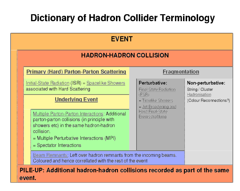
In order to interpret the detected objects in terms of the underlying short distance physics, jet algorithms are employed to associate “nearby” objects into jets. The jet algorithms are intended to cluster together the long distance particles, or energies measured in calorimeter cells, with the expectation that the kinematics (energy and momentum) of the resulting cluster or jet provides a useful measure of the kinematics (energy and momentum) of the underlying, short-distance partons. The goal is to characterize the short-distance physics, event-by-event, in terms of the discrete jets found by the algorithm. A fundamental assumption is that the basic mismatch between colored short-distance objects and the colorless long-distance objects does not present an important limitation.
As noted, jet algorithms rely on the merging of objects that are, by some measure, nearby each other. This is essential in perturbation theory where the divergent contributions from virtual diagrams must contribute in exactly the same way as the divergent contributions from soft and collinear real emissions in order that these contributions can cancel. It is only through this cancellation that jet algorithms serve to define an IR-safe (finite) quantity. The standard measures of “nearness” (see [2]) include pair-wise relative transverse momenta, as in the algorithm, or angles relative to a jet axis, as in the cone algorithm. By definition a “good” algorithm yields stable (i.e., similar) results whether it is applied to a state with just a few partons, as in NLO perturbation theory, a state with many partons after the short distance partons shower as simulated in a Monte Carlo, a state with hadrons as simulated in a Monte Carlo including a model for the hadronization step and the underlying event, or applied to the observed tracks and energy deposition in a real detector. As we will see, this constitutes a substantial challenge. Further, it is highly desirable that the identification of jets be insensitive to the contributions from the simultaneous uncorrelated soft collisions that occur during pile-up at high luminosity. Finally we want to be able to apply the same algorithm (in detail) at each level in the evolution of the hadronic final state. This implies that we must avoid components in the algorithm that make sense when applied to data but not to fixed order perturbation theory, or vice versa. This constraint will play a role in our subsequent discussion.
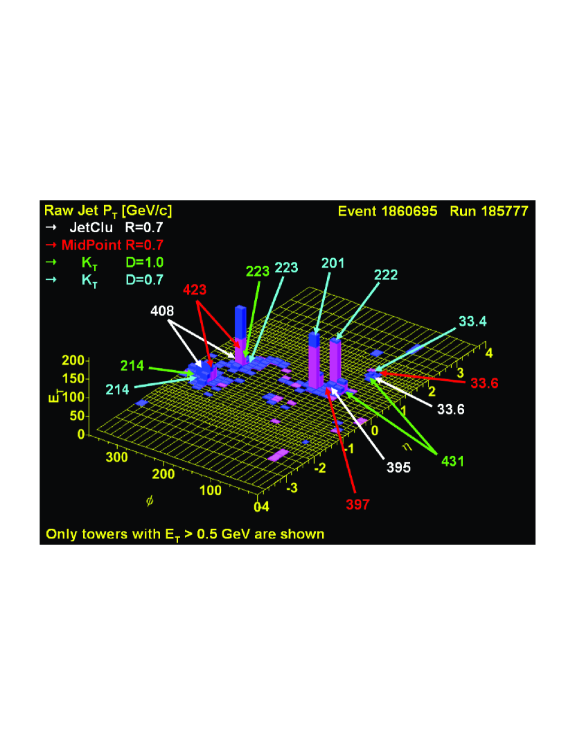
For many events, the jet structure is clear and the jets, into which the individual towers should be assigned, are fairly unambiguous, i.e. are fairly insensitive to the particular definition of a jet. However, in other events such as Fig. 2.0.2, the complexity of the energy depositions means that different algorithms will result in different assignments of towers to the various jets. This is not a problem if a similar complexity is exhibited by the theoretical calculation, which is to be compared to the data. However, the most precise and thoroughly understood theoretical calculations arise in fixed order perturbation theory, which can exhibit only limited complexity, e.g., at most two partons per jet at NLO. On the other hand, for events simulated with parton shower Monte Carlos the complexity of the final state is more realistic, but the intrinsic theoretical uncertainty is larger. Correspondingly the jets identified by the algorithms vary if we compare at the perturbative, shower, hadron and detector level. Thus it is essential to understand these limitations of jet algorithms and, as much as possible, eliminate or correct for them. It is the goal of the following discussion to highlight the issues that arose during Run I at the Tevatron and outline their current understanding and possible solution during Run II and at the LHC.
Parton Level Vs Experiment - A Brief History of Cones
The original Snowmass[3] implementation of the cone algorithm can be thought of in terms of a simple sum over all objects within a cone, centered at rapidity (the actual original version used the pseudorapidity ) and azimuthal angle and defining a -weighted centroid via
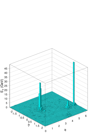
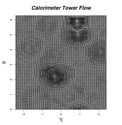
If the -weighted centroid does not coincide with the geometric center of the cone, , a cone is placed at the -weighted centroid and the calculation is repeated. This simple calculation is iterated until a “stable” cone is found, , which serves to define a jet (and the name of this algorithm as the iterative cone algorithm). Thus, at least in principle, one can think in terms of placing trial cones everywhere in and allowing them to “flow” until a stable cone or jet is found. This flow idea is illustrated in Fig, 2.0.3, where a) illustrates the LEGO plot for a simple (quiet) Monte Carlo generated event with 3 apparent jets and b) shows the corresponding flows of the trial cones. Compared to the event in Fig. 2.0.2 there is little ambiguity in this event concerning the jet structure.
To facilitate the subsequent discussion and provide some mathematical structure for this image of “flow” we define the “Snowmass potential” in terms of the 2-dimensional vector via
The flow described by the iteration process is driven by the “force”
where and is defined by . As desired, this force pushes the cone to the stable cone position.
Note that in the Run II analyses discussed below 4-vector techniques are used and the corresponding E-scheme centroid is given instead by
In the NLO perturbative calculation these changes in definitions result in only tiny numerical changes.
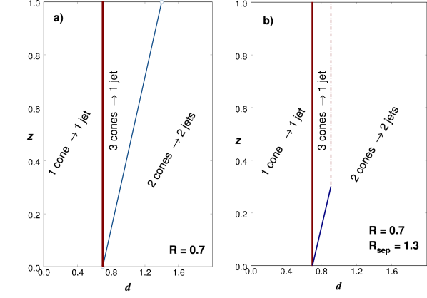
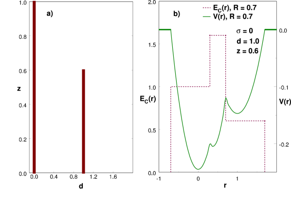
To understand how the iterative cone algorithm works consider first its application to NLO level in perturbation theory (see, e.g., [4, 5, 6, 7]), where there are most 2 partons in a cone. As defined above, the cone algorithm specifies that two partons are included in the same jet (i.e., form a stable cone) if they are both within (e.g., 0.7 in space) of the centroid, which they themselves define. This means that 2 partons of equal can form a single jet as long as their pair-wise angular separation does not exceed the boundaries of the cone, . On the other hand, as long as , there will also be stable cones centered around each of the partons. The corresponding 2-parton phase space for is illustrated in Fig. 2.0.4 a) in terms of the ratio and the angular separation variable . To the left of the line the two partons always form a single stable cone and jet, while to the far right, , there are always two distinct stable cones and jets, with a single parton in each jet. More interesting is the central region, , which exhibits both the case of two stable cones (one of the partons in each cone) and the case of three stable cones (the previous two cones plus a third cone that includes both partons). The precise outcome depends on the specific values of and . (Note that the exactly straight diagonal boundary in the figure corresponds to the -weighted definition of the Snowmass algorithm, but is only slightly distorted, , when full 4-vector kinematics is used as in the Run II algorithms.) To see the three stable cone structure in terms of the 2-parton “Snowmass potential” consider the point and , which is the 3 cones 1 jet region. The corresponding potential is illustrated in Fig. 2.0.5. This potential exhibits the expected 3 minima corresponding to a stable cone at each parton and a more central stable cone that includes both partons. A relevant point is that the central minimum is not nearly as deep (i.e., as robust) as the other two. As we shall see, this minimum often does not survive the smearing inherent in the transition from the short distances of fixed order perturbation theory to the long distances of the physical final state. As indicated by the labeling in Fig. 2.0.4, in the 3 stable cone region the original perturbative calculation[4, 5, 6, 7] kept as the jet the 2-in-1 stable cone, maximum configuration, i.e., the cone that included all of the energy in the other two cones consistent with the merging discussion below.
As we will see, much of the concern and confusion about the cone algorithm arises from the treatment of this 3 stable cone region. It is intuitively obvious that, as the energy in the short-distance partons is smeared out by subsequent showering and hadronization, the structure in this region is likely to change. In particular, while two individual, equal partons separated by nearly may define a stable cone, this configuration is unlikely to yield a stable cone after showering and hadronization.
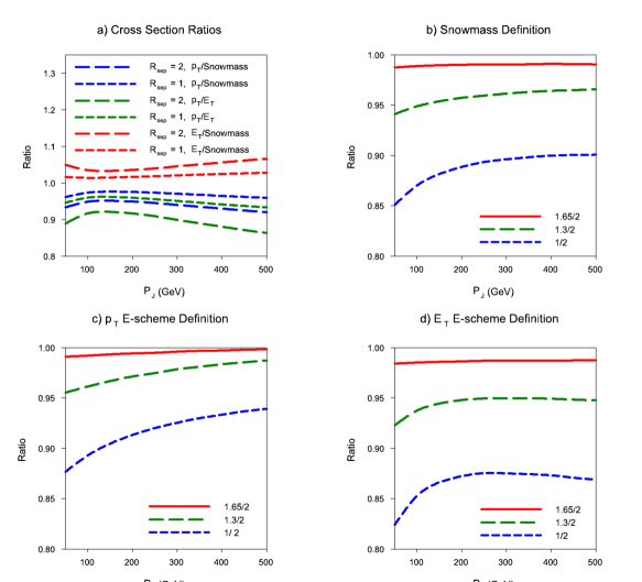
Iterative cone algorithms similar to the one just described were employed by both the CDF and DØ collaborations during Run I with considerable success. There was fairly good agreement with NLO perturbative QCD (pQCD) for the inclusive jet cross section over a dynamic range of order . During Run I the data were corrected primarily for detector effects and for the contributions of the underlying event. In fact, a positive feature of the cone algorithm is that, since the cone’s geometry in space is (meant to be) simple, the correction for the “splash-in” contribution of the (largely uncorrelated) underlying event (and pile-up) is straightforward. (As we will see below the corrections being used in Run II are more sophisticated.) The uncertainties in both the data and the theory were or greater, depending on the kinematic regime, and helped to ensure agreement. However, as cone jets were studied in more detail, various troubling issues arose. For example, it was noted long ago[8, 9] that, when using the experimental cone algorithms implemented at the Tevatron, two jets of comparable energy111These studies were performed using artificial events, constructed by overlaying jets from 2 different events in the data. The fact that these are not “real” events does not raise any serious limitations. are not merged into a single jet if they are separated by an angular distance greater than approximately 1.3 times the cone radius, while the simple picture of Fig. 2.0.4 a) suggests that merging should occur out to an angular separation of . Independently it was also noted that the dependence of the experimental inclusive jet cross section on the cone radius [10] and the shape of the energy distribution within a jet[11] both differed discernibly from the NLO predictions (the data was less dependent and exhibited less energy near the edge of the cone). All three of these issues seemed to be associated with the contribution from the perturbative configuration of two partons with comparable at opposite sides of the cone (, in Fig. 2.0.4 a)) and the data suggested a lower contribution from this configuration than present in the perturbative result. To simulate this feature in the perturbative analysis a phenomenological parameter was added to the NLO implementation of the cone algorithm[12]. In this ”experiment-aware” version of the perturbative cone algorithm two partons are not merged into a single jet if they are separated by more than from each other, independent of their individual distance from the -weighted jet centroid. Thus the two partons are merged into the same jet if they are within of the -weighted jet centroid and within of each other; otherwise the two partons are identified as separate jets. In order to describe the observed dependence of the cross section and the observed energy profile of jets the specific value was chosen (along with a “smallish” renormalization/factorization scale ), which was subsequently noted to be in good agreement with the aforementioned (independent) jet separation study. The resulting 2 parton phase space is indicated in Fig. 2.0.4 b). In the perturbative calculation, this redefinition, leading to a slightly lower average for the leading jet, lowers the NLO jet cross section by about 5% (for and GeV/c). It is important to recognize that the fractional contribution to the inclusive jet cross section of the merged 2 parton configurations in the entire wedge to the right of is only of order for jet of order 100 GeV/c, and, being proportional to , decreases with increasing . Thus it is no surprise that, although this region was apparently treated differently by the cone algorithm implementations of CDF and DØ during Run I as discussed below, there were no relevant cross section disagreements above the uncertainties. While the parameter is ad hoc and thus an undesirable complication in the perturbative jet analysis, it will serve as a useful pedagogical tool in the following discussions. To illustrate this point quantitatively Fig. 2.0.6 shows the dependence on for various choices of the jet momentum at NLO in perturbation theory. The curves labeled Snowmass use the weighted kinematics described above with given by the scalar sum of the transverse momenta of the partons in the cone. The two E-scheme algorithms use full 4-vector kinematics (as recommended for Run II in [2]) and equal to either the magnitude of the true (vector sum) transverse momentum (the recommended choice), or the “transverse energy” defined by (as defined by CDF in Run I). Thus this last variable knows about both the momentum and the invariant mass of the set of partons in the cone, which can be sizable for well separated parton pairs. The differences in the various ratios for different values of tell us about how the 2-parton configurations contribute. For example, Fig. 2.0.6 a) tells us that, since, for a given configuration of 2 partons in a cone, , the cross sections at a given value of will show the same ordering. Further, as expected, the differences are reduced if we keep only configurations with small angular separation, . From Fig. 2.0.6 b) we confirm the earlier statement that lowering from 2 to 1.3 yields a change for the Snowmass algorithm cross section with GeV, while lowering it all the way to , i.e., removing all of the triangular region, lowers the 100 GeV Snowmass jet cross section by approximately . Figs. 2.0.6 c) and d) confirm that 4-vector kinematics with exhibits the smallest sensitivity to , i.e., to the 2-parton configurations in the triangle. The choice , with its dependence on the mass of the pair, exhibits the largest sensitivity to . These are good reasons to use the recommended E-scheme kinematics with .
The difference between the perturbative implementation of the iterative cone algorithm and the experimental implementation at the Tevatron, which is simulated by , was thought to arise from several sources. While the perturbative version (with ) analytically includes all 2-parton configurations that satisfy the algorithm (recall Fig. 2.0.4 a)), the experiments employ the concept of seeds to reduce the analysis time and place trial cones only in regions of the detector where there are seeds, i.e., pre-clusters with substantial energy. This procedure introduces another parameter, the lower threshold defining the seeds, and also decreases the likelihood of finding the 2-showers-in-one-jet configurations corresponding to the upper right-hand corner of the 3 cones 1 jet region of Fig. 2.0.4 a) and the middle minimum in Fig. 2.0.5 b). Thus the use of seeds contributes to the need for . Perhaps more importantly, the desire to match theory with experiment means that we should include seeds in the perturbative algorithm. This is accomplished by placing trial cones only at the locations of each parton and testing to see if any other partons are inside of these cones. Thus at NLO, two partons will be merged into a single jet only if they are closer than in space. This corresponds to in the language of Fig. 2.0.4 and produces a larger numerical change in the analysis than observed, i.e., we wanted . More importantly at the next order in perturbation theory, NNLO, there are extra partons that can play the role of low energy seeds. The corresponding parton configurations are illustrated in Fig. 2.0.7. At NLO, or in the virtual correction in NNLO, the absence of any extra partons to serve as a seed leads to two distinct cones as on the left, while a (soft) real emission at NNLO can lead to the configuration on the right where the soft gluon “seeds” the middle cone that includes all of the partons. The resulting separation between the NNLO virtual contribution and the NNLO soft real emission contribution (i.e., they contribute to different jet configurations) leads to an undesirable logarithmic dependence on the seed threshold[13]. In the limit of an arbitrarily soft seed cutoff, the cone algorithm with seeds is no longer IR-safe. By introducing seeds in the algorithm we have introduced exactly what we want to avoid in order to be Infrared Safe, sensitivity to soft emissions. From the theory perspective seeds are a very bad component in the algorithm and should be eliminated. The labeling of the Run I cone algorithm with seeds as Infrared Unsafe has led some theorists to suggest that the corresponding analyses should be disregarded. This is too strong a reaction, especially since the numerical difference between the jet cross section found in data using seeds is expected to be less than 2% different from an analysis using a seedless algorithm. A more useful approach will be to either avoid the use of seeds, or to correct for them in the analysis of the data, which can then be compared to a perturbative analysis without seeds. We will return to this issue below.
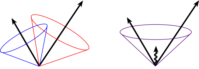
To address the issue of seeds on the experimental side and the parameter on the phenomenological side, the Run II study[2] recommended using the MidPoint Cone Algorithm, in which, having identified 2 nearby jets, one always checks for a stable cone with its center at the MidPoint between the 2 found cones. Thus, in the imagery of Fig. 2.0.7, the central stable cone is now always looked for, whether there is a actual seed there or not. It was hoped that this would remove the sensitivity to the use of seeds and remove the need for the parameter. While this expectation is fully justified with the localized, short distance configuration indicated in Fig. 2.0.7, more recent studies suggest that at least part of the difficulty with the missing stable cones at the midpoint position is due to the (real) smearing effects on the energy distribution in of showering and hadronization, as will be discussed below. Also it is important to note that, in principle, IR-safety issues due to seeds will reappear in perturbation theory at order NNNLO, where the midpoint is not the only problem configuration (a seed at the center of a triangular array of 3 hard and merge-able partons can lead to IR-sensitivity).
Before proceeding, we must consider another important issue that arises when comparing the cone algorithm applied in perturbation theory with its application to data at the Tevatron. The practical definition of jets equaling stable cones does not eliminate the possibility that the stable cones can overlap, i.e., share a subset (or even all) of their calorimeter towers. To address this ambiguity, experimental decisions had to be made as to when to completely merge the two cones (based on the level of overlap), or, if not merging, how to split the shared energy. Note that there is only a weak analogy to this overlap issue in the NLO calculation. As described in Fig. 2.0.4 a), there is no overlap in either the left-hand (1 cone 1 jet) or right-hand (2 cones 2 jets) regions, while in the middle (3 cones 1 jet) region the overlap between the 3 cones is 100% and the cones are always merged. Arguably the phenomenological parameter also serves to approximately simulate not only seeds but also the role of non-complete merging in the experimental analysis. In practice in Run I, CDF and DØ chose to use slightly different merging parameters. Thus, largely unknown to most of the theory community, the two experiments used somewhat different cone jet algorithms in Run I. (The CDF collaboration cone algorithm, JETCLU[14], also employed another “feature” called ratcheting, that was likewise under-documented. Ratcheting ensured that any calorimeter tower in an initial seed was always retained in the corresponding final jet. Stability of the final cones was partially driven by this “no-tower-left-behind” feature.)
Presumably the two experiments reported compatible jet physics result in Run I due to the substantial uncertainties. Note also that after the splitting/merging step, the resulting cone jets will not always have a simple, symmetric shape in , which complicates the task of correcting for the underlying event and leads to larger uncertainties. In any case the plan for Run II as outlined in the Run II Studies[2], called for cone jet algorithms in the two collaborations as similar as possible. Unfortunately, as described in more detail below, events during Run II have moved the collaborations off that track and they are currently employing somewhat different cone algorithms. On the merging question, CDF in Run II merges two overlapping cones when more than 75% of the smaller cone’s energy overlaps with the larger jet. When the overlap is less, the overlap towers are assigned to the nearest jet. DØ, on the other hand, uses a criterion of a 50% overlap in order to merge. While it is not necessary that all analyses use the same jet algorithm, for purposes of comparison or the combination of datasets it would be very useful for the experiments to have one truly common algorithm.
Run II Cone Algorithm Issues
In studies of the Run II cone algorithms, a previously unnoticed problem has been identified[15] at the particle and calorimeter level, which is explicitly not present at the NLO parton level. It is observed in a (relatively small) fraction of the events that some energetic particles/calorimeter towers remain unclustered in any jet. This effect is understood to arise in configurations of two nearby (i.e., nearby on the scale of the cone size) showers, where one shower is of substantially larger energy. Any trial cone at the location of the lower energy shower will include contributions from the larger energy shower, and the resulting -weighted centroid will migrate towards the larger energy peak. This feature is labeled “dark towers” in Ref. [15], i.e., clusters that have a transverse momentum large enough to be designated either a separate jet or to be included in an existing nearby jet, but which are not clustered into either. A Monte Carlo event with this structure is shown in Fig. 2.0.8, where the towers unclustered into any jet are shaded black.
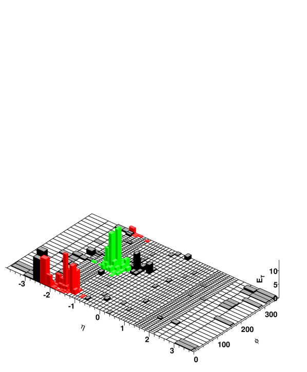
A simple way of understanding the dark towers can be motivated by returning to Fig. 2.0.5, where the only smearing in between the localized energy distribution of part a) (the individual partons) and the “potential” of part b) arises from the size of the cone itself. On the other hand, we know that showering and hadronization will lead to further smearing of the energy distribution and thus of the potential. Sketched in Fig. 2.0.9 is the potential (and the energy-in-cone) distributions that results from Gaussian smearing with a width of a) and b) (in the same angular units as ). In both panels, as in Fig. 2.0.5, the partons have ratio and angular separation . Note that as the smearing increases from zero as in panel a), we first lose the (not so deep) minimum corresponding to the midpoint stable cone (and jet), providing another piece of the explanation for why showers more than apart are not observed to merge by the experiments. In panel b), with even more smearing, the minimum in the potential near the shower from the lower energy parton also vanishes, meaning this (lower energy) shower is part of no stable cone or jet, i.e., leading to dark towers. Any attempt to place the center of a trial cone at the position of the right parton will result in the centroid “flowing” to the position of the left parton and the energy corresponding to the right parton remaining unclustered in any jet. (Note that the Run I CDF algorithm, JETCLU with Ratcheting, limited the role of dark towers by never allowing a trial cone to leave the seed towers, the potential dark towers, behind.) The effective smearing in the data is expected to lie between values of 0.1 and 0.25 (with shower-to-shower fluctuations and some energy dependence, being larger for smaller jets) making this discussion relevant, but this question awaits further study as outlined below. Note that Fig. 2.0.9 also suggests that the Midpoint algorithm will not entirely fix the original issue of missing merged jets. Due to the presence of (real) smearing this middle cone is almost never stable and the merged jet configuration will not be found even though we have explicitly looked for it with the midpoint cone. Thus even using the recommended Midpoint algorithm (with seeds), as the DØ collaboration is doing (with the also recommended value), there may remain a phenomenological need for the parameter value .
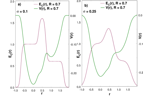
A potential solution for the dark towers problem is described in Ref. [15]. The idea is to decouple the jet finding step from the jet construction step. In particular, the stable cone finding procedure is performed with a cone of radius half that of the final jet radius, i.e., the radius of the search cone, . This procedure reduces the smearing in Figs. 2.0.5 and 2.0.9, and reduces the phase space for configurations that lead to dark towers (and missing merged jets).
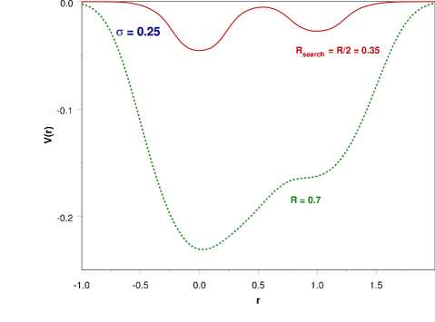
This point is illustrated in Fig. 2.0.10, which shows the potential of Fig. 2.0.9, panel b) corresponding to the reduced radius search cone. Note, in particular, that there is again a minimum at the location of the second parton. Seeds placed at each parton will yield a stable cone at each location even after the smearing. Using the smaller search cone size means there is less influence from the (smeared) energy of nearby partons. After identifying the locations of stable cones, the larger cone size, e.g., , is used to sum all objects inside and construct the energy and momentum of the jet (with no iteration). All pairs of stable cones separated by less than are then used to define midpoint seeds as in the usual MidPoint Cone Algorithm. A trial cone of size is placed at each such seed and iterated to test for stability. (Note that this midpoint cone is iterated with cone size , not the smaller , contrary to what is described in the literature.) Thus, just as in the MidPoint Cone Algorithm, stable midpoint cones will be found by the CDF Search Cone Algorithm. However, as already discussed, we expect that there will be no stable midpoint cone due to the smearing. Note that, even with the reduced smearing when using the smaller search cone radius, there is still no central stable cone in the potential of Fig. 2.0.10. On the other hand, as applied to NLO perturbation theory without smearing, the Search Cone Algorithm should act like the usual MidPoint Cone Algorithm and yield the naïve result of Fig. 2.0.4 a). The net impact of adding the step with the smaller initial search cone as applied to data is an approximately 5% increase in the inclusive jet cross section. In fact, as applied to data the Search Cone Algorithm identifies so many more stable cones, that the CDF collaboration has decided to use the Search Cone Algorithm with the merging parameter (instead of ) to limit the level of merging.
Unfortunately a disturbing feature of the Search Cone Algorithm arises when it is applied at higher orders in perturbation theory as was pointed out during this Workshop[16]. At NNLO in perturbation theory the Search Cone Algorithm can act much like the seeds discussed earlier. In particular, the search cone algorithm can identify a (small, radius ) stable (soft) cone between two energetic cones, exactly the soft gluon between 2 energetic partons configuration discussed earlier. The soft search cone is stable exactly because it “fits” between the two energetic partons without including either; the spacing between the two energetic partons can be in the range . Then, when the radius of the (stable, soft) search cone is increased to , the resulting full size cone will envelop, and serve to merge, the two energetic partons. This can occur even when the two energetic partons do not constitute a stable combined cone in the standard cone algorithm. Thus at NNLO the search cone algorithm can exhibit an IR-sensitivity very similar to, and just as undesirable as, the seed-induced problem discussed earlier. The conclusion is that the search cone algorithm, while it does address the dark tower issue, creates its own set of issues and is not considered to be a real solution of the dark tower problem.
In summary, the DØ collaboration is using the Midpoint Cone algorithm with (and seeds) to analyze Run II data, while the CDF collaboration is using the Search Cone algorithm with (with seeds). CDF is encouraged to return to also using the Midpoint Cone algorithm. The two collaborations are encouraged to determine an optimum value of that is both common and appropriate to future high luminosity running. To compare fixed order perturbation theory with data there must be corrections for detector effects, for the splash-in contributions of the underlying event (and pile-up) and for the splash-out effects of showering and hadronization. It is the response to these last effects that distinguishes the various cone algorithms and drives the issues we have just been discussing. The fact that the splash-in and splash-out corrections come with opposite signs and can cancel in the uncorrected data for the inclusive jet cross section, may help explain why Run I comparisons with perturbation theory sometimes seemed to be better than was justified (with hindsight). We will return to the question of Run II corrections below. The conclusion from the previous discussion is that it would be very helpful to include also a correction in the experimental analysis that accounts for the use of seeds. Then these experimental results could be compared to perturbative results without seeds avoiding the inherent infrared problems caused by seeds in perturbative analyses. At the same time, the analysis described above suggests that using the MidPoint Cone Algorithm, to remove the impact of seeds at NLO, does not eliminate the impact of the smearing due to showering and hadronization, which serves to render the midpoint cone of fixed order perturbation theory unstable. Thus we should still not expect to be able to compare data to NLO theory with (in Run II analyses DØ is comparing to NLO with , while CDF is still using ).
kT Algorithms
With this mixed history of success for the cone algorithm, the (as yet) less well studied algorithm[17, 18, 19] apparently continues to offer the possibility of nearly identical analyses in both experiments and in perturbation theory. Indeed, the algorithm, which was first used in electron-positron colliders, appears to be conceptually simpler at all levels. Two partons/particles/calorimeter towers are combined if their relative transverse momentum is less than a given measure. To illustrate the clustering process, consider a multi-parton final state. Initially each parton is considered as a proto-jet. The quantities and are computed for each parton and each pair of partons , respectively. As earlier is the transverse momentum of the parton, is the distance (in space, ) between each pair of partons. is the parameter that controls the size of the jet (analogous to ). If the smallest of the above quantities is a , then that parton becomes a jet and is removed from the proto-jet list. If the smallest quantity is a , then the two partons are merged into a single proto-jet by summing their four-vector components, and the two original entries in the proto-jet list are replaced by this single merged entry. This process is iterated with the corrected proto-jet list until all the proto-jets have become jets, i.e., at the last step the for all pairs of proto-jets are larger than all for the proto-jets individually (i.e., the remaining proto-jets are well separated) and the latter all become jets.
Note that in the pQCD NLO inclusive jet calculation, the parton pair with the smallest may or may not be combined into a single jet, depending on the of the individual partons. Thus the final state can consist of either 2 or 3 jets, as was also the case for the cone algorithm. In fact, the pQCD NLO result for the inclusive jet cross section[17] suggests near equality with the cone jet cross section in the case that (with no seeds, ). Thus the inclusive cone jet cross section with () is comparable in magnitude to the inclusive jet cross section with , at least at NLO. In the NLO language illustrated in Fig. 2.0.4 the condition that the partons be merged in the algorithm is that or . Thus at NLO the algorithm corresponds to the cone algorithm with , . The earlier result, (with ), is just the NLO statement that the contribution of the rectangular region , is numerically approximately equal to the contribution of the rectangular region , plus the (3 stable cone) triangular region , .
In contrast to the cone case, the algorithm has no problems with overlapping jets and, less positively, every calorimeter tower is assigned to some jet. While this last result made some sense in the collider case, where every final state particle arose from the short-distance process, it is less obviously desirable in the hadron collider case. While the algorithm tends to automatically correct for the splash-out effect by re-merging the energy distribution smeared by showering and hadronization into a single jet, this same feature leads to a tendency to enhance the splash-in effect by ”vacuuming up” the contributions from the underlying event and including them in the large jets. This issue is exacerbated when the luminosity reaches the point that there is more than one collision per beam bunch crossing and pile-up is significant. This is now true at the Tevatron and will certainly be true eventually at the LHC. Thus while the (splash-out) fragmentation corrections for the algorithm are expected to be smaller than for cone algorithms, the (splash-in) underlying event corrections will be larger. This point presumably provides at least a partial explanation for the only marginal agreement between theory and experiment in the Run I results with the algorithm from the DØ Collaboration[20]. A test of our understanding of these corrections will be provided by the comparison of the and parameter values that yield comparable experimental jet cross sections. If we can reliably correct back to the fixed order perturbative level for both the cone and algorithms, we should see . Note that this result assumes that the cone jet cross section has been corrected to the value corresponding to . On the other hand, under-corrected splash-in contributions in the algorithm will require for comparable jet cross section values (still assuming that describes the cone results). If the cone algorithm jet cross section has under-corrected splash-out effects (), we expect that an even smaller ratio of to will required to obtain comparable jet cross sections (crudely we expect for ).
Another concern with the algorithm is the computer time needed to perform multiple evaluations of the list of pairs of proto-jets as 1 pair is merged with each pass, leading to a time that grows as , where is the number of initial proto-jets in the event. Recently[21] an improved version of the algorithm has been defined that recalculates only an intelligently chosen sub-list with each pass and the time grows only as , for large .
It should also be noted that, although it would appear that the algorithm is defined by a single parameter , the suggested code for the algorithm on its “official” web page[22] includes 5 parameters to fully define the specific implementation of the algorithm. Thus, as is the case for the cone algorithm, the algorithm also exhibits opportunities for divergence between the implementation of the algorithm in the various experiments, and care should be taken to avoid this outcome.
Run II Jet Results
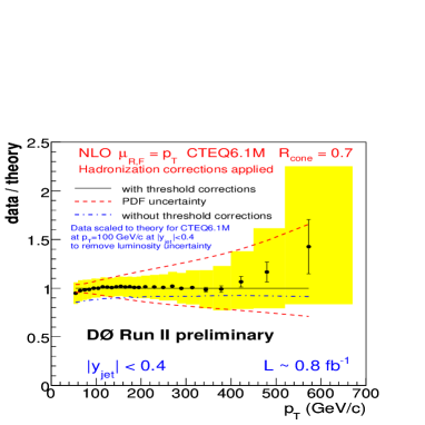
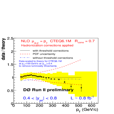
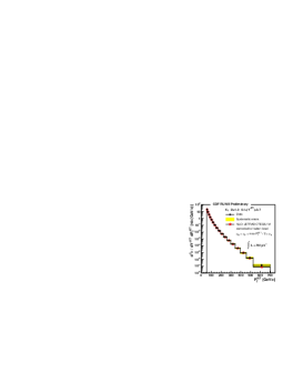
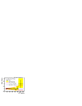
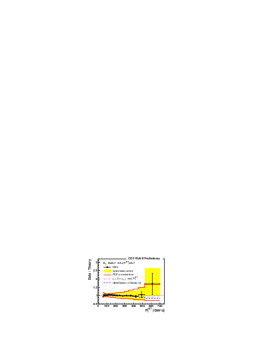
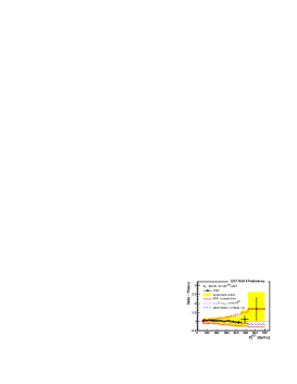
Preliminary Run II inclusive cone jet results[23, 24] suggest that, even with differing algorithms, the two collaborations are in reasonable agreement as indicated in Figs. 2.0.11 and 2.0.12. On the other hand, the challenge, as noted above, is to continue to reduce the systematic uncertainties below the current 10% to 50% level, which effectively guarantees agreement, if the primary differences are also at the 10% level. Indeed, the current studies of the corrections due to splash-in, i.e., the underlying event (and pile-up), and the splash-out corrections due to hadronization are much more sophisticated than in Run I and presented in such a way that they can be applied either to the data (corrected for the detector) or to a theoretical (perturbative) calculation. The evaluation of these corrections is based on data and the standard Monte Carlos, PYTHIA and HERWIG, especially Tune A of PYTHIA, which seems to accurately simulate the underlying event in terms of multiple parton interactions, including the observed correlations with the hard scattering process.[25]

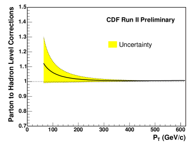
For CDF the multiple interaction (pile-up) correction is measured by considering the minimum bias momentum in a cone placed randomly in with the constraint that (so the rapidity range matches the range for the jet cross section measurement). The in the cone is measured as a function of the number of vertices in the event. The slope, , of the straight line fit to versus the number of vertices is the that needs to be removed from the raw jet for each additional vertex seen in an event, where the number of vertices is proportional to the number of additional interactions per crossing. The measurement of the correction is therefore affected by fake vertices. The correction to the inclusive jet cross section decreases as the jet increases. The towers that are within the cone are summed as 4-vectors just as in the Midpoint jet algorithm. The summation of the towers uses the following prescription: for each tower construct the 4-vectors for the hadronic and electromagnetic compartments of the calorimeter (correctly accounting for the location of the z-vertex). The 4-vectors are then summed. This method, while it does approximate the Midpoint algorithm, makes no attempt to account for the splitting/merging that is performed by the cone jet algorithm (resulting in jets that are not shaped like ideal cones). This random cone method is a reasonable approach when the number of additional interactions is small. At CDF, the correction to a Midpoint jet (cone radius of 0.7) is GeV/c per jet. The effect of this correction is significantly different if there is 1 additional vertex per event than if there are 10. It may be the case that for a large number of additional vertices the systematic uncertainty associated with the pile up correction may become comparable to the other systematic uncertainties. The systematic uncertainty assigned to this correction is determined in part by its inclusion in the generic correction scheme used by CDF. The systematic uncertainty is made large enough to cover the variation of correction as derived in different samples. Note that the jet clustering has a threshold of 100 MeV, towers below this are not included in any jet. Additional energy deposited in a cone can be added to a tower below threshold and thus cause it to be included in the jet or be added to a tower that was already in the jet. Following the methods used in Run I, the correction for pile up was derived with 3 tower thresholds, 50 MeV, 100 MeV, and 150 MeV, which provides some check of the two ways that the pile up energy can be added to a tower. An alternative approach is to derive the correction based on making the shape of the inclusive cross section independent of the instantaneous luminosity (and this approach has been used to compare the corrections in the cone algorithm with those in the algorithm).
The CDF hadronization correction (parton to hadron as described here) for the inclusive jet cross section (cone or ) is obtained using PYTHIA (Tune A), as noted above. The correction is simply the ratio of the hadron level inclusive jet cross section with multiple parton interactions (MPI) turned on over the parton level (after showering) inclusive jet cross section with MPI turned off. This results in a correction (for the Search Cone algorithm) at 60 GeV/c. Although it is unphysical to explicitly separate the effects of organizing the partons into hadrons and including the contributions of the underlying event (UE), it is still a useful approximation in the context of the Monte Carlos and produces fairly stable and intuitively appealing results. Further, since only an underlying event correction was employed in the Run I analyses, the option to apply just the underlying event correction provides a connection between the results from the 2 runs. The underlying event correction found in this way corresponds to adding approximately 1 GeV to the perturbative jet, crudely in agreement with the Run I numbers. The definitions for the separate corrections are as follows:
In these expressions, UE means MPI turned on, no-UE means MPI turned off. The beam-beam remnants in PYTHIA tend to end up at large rapidity and their effect on the central rapidity jet cross section is not included here. The systematic uncertainty assigned to the hadronization correction comes from comparing, in PYTHIA and HERWIG, the fragmentation and UE components. PYTHIA and HERWIG have very similar fragmentation corrections. However, as expected, the UE corrections are different. The resulting systematic uncertainty comes exclusively from the different UE correction and was found to be for jets near 60 GeV/c.
CDF has also undertaken a similar study of corrections for the algorithm[26]. In this case, without the fixed geometry of the cone algorithm, the multiple interaction correction is extracted from the data by asking that the shape of the measured inclusive jet cross section be independent of the instantaneous luminosity after the correction is applied. It was also confirmed that, within systematic uncertainties, the corrections are consistent between the cone and algorithms for . As a further test the luminosity independent inclusive jet cross section shape test (after correction) was applied also to the cone algorithm. This approach yields only a slightly larger correction than found by the method above using minimum bias events, and still within the expected systematic uncertainty. The slightly larger correction is presumably due to the remaining effects from merging/splitting of the cones. As mentioned above, the algorithm hadronization correction is determined just as in the cone algorithm case. The resulting corrections yield quite satisfactory agreement between the corrected theory and experiment as indicated in Fig. 2.0.13 for a range of values of . This figure also exhibits the quite substantial systematic uncertainty in these corrections (of order 50% to 80% of the correction) and an overall systematic uncertainty (see the middle row of graphs in Fig. 2.0.13) of order 20% at low to close to 100% at large . Thus the current systematic uncertainty of the algorithm results are comparable to those for the cone algorithm, as indicated in Figs. 2.0.11 and 2.0.12.


Non-perturbative contributions to jet measurements
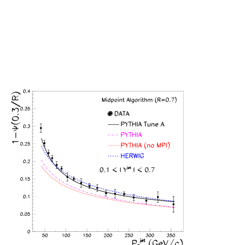
As noted above, in hadron-hadron collisions, the measured inclusive jet production cross section at the particle level, regardless of the jet algorithm considered, includes all-orders and non-perturbative contributions from the underlying event and the fragmentation into hadrons that are not present in the fixed-order parton-level calculation, which become significant at low jet transverse momentum. A proper comparison between the data and the theoretical prediction requires good control of such contributions. Experimentally, they are estimated using leading-order parton-shower Monte Carlo generators, and the variation of the predicted jet cross sections after turning off the interaction between beam remnants and the hadronization in the Monte Carlo. This procedure is model dependent, and strongly relies on the Monte Carlo providing a good description of those observables in the data that are most sensitive to non-perturbative contributions like, for example, the internal structure of the jets. Recent precise measurements on jet shapes[27], as indicated in Fig. 2.0.14, have allowed the detailed study of the models employed to describe the underlying event in inclusive jet production at the Tevatron (see also Ref. [25]). Future measurements of the underlying event in Run II, for different hadronic final states, promise to play a major role in the early understanding of the measured jet cross sections at the LHC.
More details
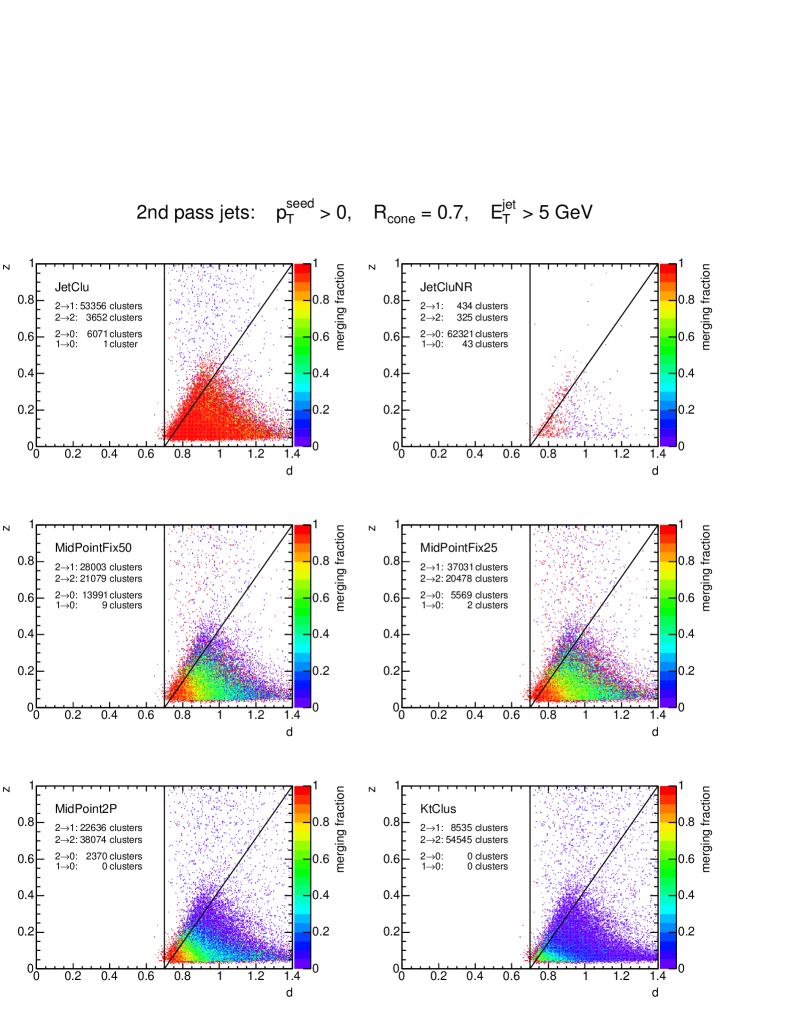
Several of the issues noted above are illustrated in Fig. 2.0.15, taken from a recent analysis[28]. The goal of the analysis, and the figure, is to understand how various cone jet algorithms deal with the issues leading to the dark towers, i.e., with configurations of nearby showers described in the notation of Fig. 2.0.4. The reference algorithm is the standard MidPoint Cone Algorithm with a seed tower threshold of 1 GeV and applied to a set of events simulated with PYTHIA (Tune A) using CTEQ5L parton distribution functions. After stable cones and jets are found, defining the 1st pass jets, the towers in these jets are removed from the analysis. The remaining towers, the dark towers, are then identified into 2nd pass jets by simply placing a cone of size 0.7 about the highest tower, calling that a 2nd pass jet and removing the enclosed towers from the analysis as long as the total in the cone is greater than 5 GeV. This process is repeated to generate the list of 2nd pass jets. For simplicity the 2nd pass jets are constructed without iteration or splitting/merging. The 2nd pass jets can be thought of as populating the plane around the closest 1st pass jet. Recall that is the angular separation and is the ratio (). Next apply the 6 other jet algorithms to the same data. JETCLU is the CDF Run I algorithm (with ratcheting and ); JETCLUNR is the same algorithm but without ratcheting; MidPointFix50 is a Search Cone Algorithm with and ; MidPointFix25 is a Search Cone Algorithm with and . The MidPoint2P algorithm, which also uses , is similar to the reference (standard) MidPoint algorithm with a 2nd pass, except that in this case the 2nd pass cones (with the 1st pass towers removed) are iterated and a midpoint stable cone is looked for. In the final step of MidPoint2P the contents of the 2nd pass cones are calculated using all towers, but no iteration, and then standard splitting/merging is applied to both 1st and 2nd pass cones. The final case studied is the Algorithm with .
To produce the plot the jets found by each of these 6 algorithms are identified with the 2nd pass and closest 1st pass jets found by the reference algorithm by comparing the highest towers. For example, if the highest towers in both a 2nd pass jet and the closest 1st pass jet are in the same JETCLU jet, we conclude that JETCLU merges these 2 clusters (a clustering). If the highest towers in both a 2nd pass jet and the closest 1st pass jet are in different JETCLU jets, we conclude that JETCLU does not merge these 2 clusters (a clustering). If the highest tower in a 2nd pass jet is not in any JETCLU jet, we conclude that it remains a dark tower also in JETCLU (a clustering). The final, unlikely scenario is that the highest tower in a 1st pass jet is not in any JETCLU jet and we conclude that JETCLU is ignoring this 1st pass jet (a clustering). Applying the same tests to each of the 6 algorithms yields the plot in Fig. 2.0.15 which compares the amount of (relative probability of) merging and splitting for the various algorithms. The total numbers of cluster pairs in each category are also listed for each algorithm on the individual plots. An “ideal” cone jet algorithm, i.e., one that matches well to NLO perturbation theory, will exhibit a large merging fraction (red) in the triangular region above the diagonal, a low merging fraction (blue) below the diagonal and few remaining dark towers. The JETCLU algorithm exhibits considerable merging everywhere, especially below the diagonal, presumably due to ratcheting. In contrast JETCLUNR without ratcheting exhibits little merging and yields essentially the same dark tower content as the reference MidPoint Cone Algorithm (i.e., mostly clustering). Thus, while ratcheting ensures a low level of clustering, i.e., few dark towers, the high level of merging over the entire region is undesirable. The MidPoint Fix25 algorithm, the one currently in use at CDF (except here instead of 0.75), has the desirable features of relatively low merging below the diagonal and relatively high merging above the diagonal with few remaining dark towers. This explains the original appeal of the search cone algorithm, but, of course, the current analysis does not speak to the IR-sensitivity issue for this algorithm when applied to perturbation theory. Similar comments apply also to the MidPointFix50 algorithm, but with somewhat less merging and more remaining dark towers. The MidPoint2P algorithm has a lower level of overall merging (a lower clustering count and a higher clustering count), and a lower number of remaining dark towers. This suggests that using a 2nd pass to find jets can address the dark tower issue. However, this approach does not address the problem of the 2-in-1 stable cone solutions that disappear when the smearing effect of fragmentation is included. This conclusion again emphasizes the difficulty of matching the behavior of jet algorithms at the parton and hadron levels. The final plot for the Algorithm illustrates the expected result that this algorithm yields very little merging of objects separated by an angular distance of more than , i.e., it acts like a cone algorithm with .
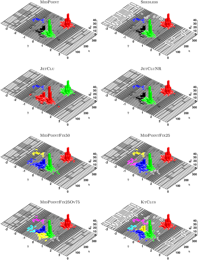
In our discussions above about of how well jet algorithms are working at the Tevatron Run II, we saw that there are detectable differences (10%) between the CDF and DØ implementations of the cone algorithm. These differences arise to a large extent from how the jet algorithms handle configurations where two energetic partons are nearby each other in on the scale of the cone size , i.e., nearby but not collinear. As suggested by the simulated event shown in Fig. 2.0.16, in general the legacy CDF algorithm JETCLU will merge the showers from the two partons (consider in particular the two tower configuration near rapidity , azimuth ) as the ratcheting feature can lead to a stable central cone, while the lower energy shower is left as dark towers when ratcheting is turned off (JetCluNR). The Run II Midpoint Cone Algorithm and the seedless algorithm likewise find only the more energetic jet with the secondary shower not included in any jet (i.e., as dark towers). The two Search Cone Algorithms (MidPointFix50 and MidPointFix25, both with ), identify the secondary shower as a second jet with some differences in the very low energy objects. The Search Cone Algorithm with (MidPointFix25Ov75, which is essentially the current CDF algorithm) finds the secondary shower to be two jets, i.e., showing less merging. Finally the Algorithm identifies all energetic towers into jets with less merging than the cone algorithms with , and only small differences from the algorithm.
The Future
In order to study the jet algorithm situation more thoroughly, we desire an analysis tool that provides NLO accuracy for the jets, i.e., reduced factorization scale dependence (suggesting small theoretical uncertainty), plus an accurate treatment of energetic radiation at angles of order with respect to the core shower direction. At the same time we must include both showering and hadronization. This is just what the development of MC/NLO tools (such as MC@NLO [29, 30]) is meant to do for us. The challenge with light jet calculations in MC/NLO is that, since every object participating in the short-distance process is colored, they can all produce their own shower. Thus the subtraction process outlined in Refs.[29, 30] must be performed for every parton and, to some extent, tuned to minimize the occurrence of events with negative weights. Note that the early work in this field focused on processes with color only in the initial state in order to minimize the required “bookkeeping”. Only recently, with the addition of the single top process[31, 32], where the top quark has essentially no time to radiate before it decays, have colored objects been included in the final state. It is now time to develop the full light jet MC@NLO code so that the optimization of the jet algorithm can be studied. Such code would allow detailed analyses of the corrections necessary to go from the long distance hadronic states measured in the detectors back to the NLO short distance partonic states of perturbation theory. Such studies could illuminate the dependence on various experimental analysis parameters that are currently largely hidden from view. For example, how much does the final jet cross section depend of the parameter used in the split/merge step of the cone algorithm. As noted above, CDF and DØ are currently using different values for this parameter. Similarly there is a question about how energetic a stable cone must be () in order to be included in the split/merge process. CDF includes all stable cones (), while DØ includes only those above 3 GeV (). It is important that we understand quantitatively the impact of the different choices for both these parameters. Their effects are certainly correlated.
Another possible avenue of study is to apply the recent progress in understanding the associated energy in events with jets, which grew out of earlier work in the study of event shapes in collisions. This work, by a variety of theorists[33, 34, 35, 36], will not be reviewed here, except to suggest its useful further application to jet issues at the Tevatron and the LHC.
A quite different approach that deserves further study is the possibility that hard scattering events can be usefully studied without the need to identify a discrete set of jets, as we have assumed here from the outset. The general idea is that the same information now carried by the jets could instead be encoded in a distribution describing the energy flow, event-by-event, removing the need to identify specific jets in each event. Recall that this is where the problems arise in the discussion above. The general idea for this approach was outlined at Snowmass 2001[37] and is touched on in some of the previously mentioned references[33, 34, 35, 36].
We close this discussion of the future with a suggestion, which arose during this Workshop, concerning how the information currently lost in the dark towers can be preserved and subsequently used in analyses. In the study leading to Fig. 2.0.15 the concepts of 1st and 2nd pass jets was introduced. Here we outline a similar 2nd pass jet algorithm in more detail. In the first step we apply the “standard” Midpoint Cone Algorithm as recommended in the Run II Workshop[2] (keeping in mind that there are differences in the current implementations). This step includes the full algorithm, including the iterative procedures to find stable cone solutions around the seeds, and later around the midpoints. It also includes the full split/merge procedure. The resulting identified jets are labeled 1st pass jets. As we have discussed, while this step produces well-defined jets, it sometimes leaves substantial amounts of energy in the event unclustered. To characterize this unclustered energy we identify it as jets in a second pass using exactly the same algorithm, but applied to the final state after all particles/towers assigned to one of the 1st pass jets are removed. These new jets are labeled 2nd pass jets.
Clearly these 2nd pass jets do not stand on the same footing as the 1st pass jets. They do not correspond to stable cone solutions when considering the full final state. Therefore there are various possibilities for making use of the 2nd pass jets. One might simply keep the 2nd pass jets as separate jets, in addition to the 1st pass jets. Since the second pass jets are typically of much smaller energy than the 1st pass jets, this will have little numerical impact on the jet cross section. This point is illustrated in Fig. 2.0.17, where the individual spectra of 1st and 2nd pass jets found in the fashion described above are displayed. A more interesting question is whether a 2nd pass jet can/should be merged with the nearest 1st pass jet (the 2nd pass jets are almost always produced within to a 1st pass jet). For example, we could merge according to the NLO structure in Fig. 2.0.4, and in this way define a dark tower correction. Based on the recent studies of the dark tower issue, we expect the correction of the inclusive single jet cross section to be of order a few percent (i.e., a substantially larger effect than simply including the 2nd pass jets in the single jet sample). Alternatively, we might study how the 2nd pass jets could be used in the reconstruction of interesting physics objects, such as highly boosted ’s, ’s and top quarks, that decay into a 1st pass jets plus a 2nd pass jet.
We recommend that studies of all of these ideas be carried out so that quantitative conclusions can be reached as to the best way to make use of the information carried by the 2nd pass jets. Such studies may benefit from employing the MC@NLO tool mentioned above.
Summary
We have come a long way in our understanding of jet algorithms and their limitations. We still have a way to go if we want to guarantee a precision much better than 10%. Overall, we expect both cone and algorithms to be useful at the LHC. Their differing strengths and weaknesses will provide useful cross checks. Our conclusions and recommendations include the following.
-
•
Seeds introduce undesirable IR sensitivity when used in theoretical calculations. The cone algorithm without seeds is IR-safe. Experimental results for the cone algorithm should be corrected for any use of seeds and compared to theoretical results without seeds.
-
•
More study is required to understand the quantitative impact and possible optimization of the choices for the parameters in the split/merge step of the cone algorithm, and . As in Run I, CDF and DØ are currently using different parameter choices and the implied differences in jet rates are not well documented. The studies aimed at finding optimal choices for the split/merge parameters should include participation by the LHC collaborations to ensure relevance to the LHC environment and an enhanced level of commonality in those experiments.
-
•
The unclustered energy in the dark towers sometimes found when using a cone algorithm requires further study. This issue is now understood to arise from the smearing effects of showering and hadronization. The Search Cone Algorithm currently employed by CDF is not a satisfactory solution to this problem and its use should be discontinued. An alternative approach using 2nd pass jets is outlined in this report and deserves further study.
-
•
Most of the challenges found in using cone algorithms are now understood to arise from the kinematic regime of two nearby (but not collinear) short-distance partons, especially as this configuration is smeared by subsequent showering and hadronization. It is precisely these effects that lead to the observation that the ad hoc phenomenological parameter requires a value less than the default value of . With the imminent appearance of MC@NLO code for jets a substantially improved analysis of this situation will be possible.
-
•
With the limitations of cone algorithms now fairly well understood and mostly correctable to the few percent level, it is extremely important that we achieve a comparable level of maturity in our understanding of the algorithm. By its nature, the algorithm will not suffer from the same issues as cone algorithms. The most pressing question, unanswered by the use of the algorithm at and colliders, is how the algorithm responds to the noisier environment of high energy, high luminosity collisions. By definition the algorithm clusters all energy into jets and the central issue is whether the contributions of the underlying event and pile-up will lead to troublesome fluctuations in the properties of algorithm jets primarily associated with the true short-distance scattering process. Thorough studies of the algorithm during Run II are essential to our preparations for the LHC. These studies should enlist participation from the LHC collaborations to ensure relevance to the even noisier environment expected at LHC energies and luminosities.
-
•
Experimental results need to be reported at the hadron level or higher; corrections between the parton level and hadron level need to be clearly specified, including uncertainties.
3 Parton Distribution Functions
3.1 Heavy Flavor Parton Distributions and Collider Physics
Contributed by: Tung
Motivation
Heavy flavor parton distributions represent an important unchartered territory in the landscape of global QCD analysis of the parton structure of the nucleon. On one hand, since they make relatively small contributions to the conventional Standard Model processes that contribute to global QCD analyses, there exist almost no hard experimental constraints on these distributions. On the other hand, their influence on physics analyses of the next generation of Collider Physics is expected to be increasingly significant— directly for Top and Higgs studies, and hence indirectly for New Physics searches. [38, 39]
Conventional global QCD analyses include heavy flavor partons, i.e. charm, bottom (and, optionally, top), under the key assumption that these partons are “radiatively generated” by QCD evolution—mainly gluon splitting. The rationale for this assumption is twofold: heavy quarks should be decoupled at low energy scales where non-perturbative light parton distributions are normally parametrized; and if the mass of the quark is much larger then , then heavy quark effects should be calculable perturbatively. Thus, in the parton parameter space, no degrees of freedom are associated with heavy flavors in all conventional analyses. While this assumption certainly is reasonable for the top quark, it is obviously questionable for the charm quark since its mass is comparable to that of the nucleon, the existence of which is definitely non-perturbative. The bottom quark case lies in-between.
There are a number of models for heavy flavor parton distributions, particularly the charm distribution, in the literature. Most anticipate distinctive non-perturbative components that are significant mainly in the large- region. However, throughout the history of global QCD analysis of parton distributions, nature has repeatedly surprised us about the flavor dependence of the sea-quarks inside the nucleon. In spite of more than 20 years of continuing efforts, large uncertainties remain even for the strange quark distribution (in addition to the gluon).
It is thus important to follow a model-independent approach in exploring the heavy flavor frontier, keeping an open mind on the range of possibilities—not just for the charm, but also for the bottom, which plays a particularly significant role in Top/Higgs physics and beyond.
Opportunities
Available data on deep inelastic scattering and production of Drell-Yan pairs, jets, and W/Z’s—the conventional sources of parton distribution determination—are not sensitive to the relatively small charm/bottom constituents of the nucleon. Heavy flavor production at HERA offer some limited constraints. To gain quantitative information, one needs to look at new channels opened up in the hadron colliders themselves. In particular, it has been known (and repeatedly emphasized, e.g. [40]) for some time, final states of /W/Z plus a tagged heavy-quark jet are directly sensitive to individual parton distributions, depending on which channel is measured. Cf. 3.1.18.
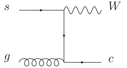
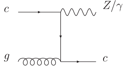

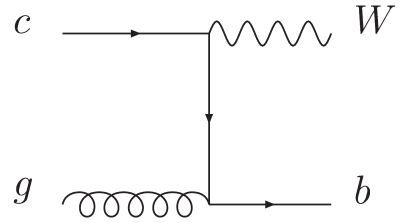
At Run II of the Tevatron, and at LHC, these are challenging measurements. But they are unique, fundamental processes that contain information about the heavy flavors not available elsewhere. Therefore, these measurements should command high priority in the overall physics program at both colliders.
On the theory side, the treatment of heavy quarks in pQCD had followed two distinct, seemingly contradictory, paths, resulting in considerable confusion in the field. On one hand, order-by-order calculations of heavy quark production cross-section were mainly carried out in the so-called fixed-flavor-number scheme (FFNS), based on the premise that the relevant quark mass is the largest scale in the process. Whereas this assumption considerably simplifies the calculation, it is clearly an inappropriate approximation in the high energy regime where the typical energy scale is larger than the quark mass (for both charm and bottom). On the other hand, most practical parton model calculations (global analyses, event generators, etc.) are carried out in the variable-flavor-number scheme (VFNS), in which charm and bottom are put on the same footing as the light quarks (i.e. zero mass) above a scale comparable to their respective mass. Although this is a reasonable description over most high energy regime, it becomes untenable at scales comparable to the mass (where much of the input experimental data for global PDF analysis lie). This dichotomy is naturally resolved in a generalized pQCD framework, most precisely formulated by Collins [41, 42, 43], based on an elegant composite renormalization scheme (CWZ [44], dating back to the 70’s). The extensive recent literature on heavy quark production, sometime described as “fixed-order plus resummation” [38, 39], are all specific implementations of the general principles of this formalism.
Although the theoretical issues have thus been clarified already for quite some time[42], and some aspects of the new insight have been adopted in many recent calculations in a variety of guises [39], a comprehensive global analysis based on the general theory incorporating the heavy quark degrees of freedom has not been carried out. However, the importance of the heavy quark sector for LHC physics is beginning to inspire more focused study on this frontier. [45]
Strategy and First Results
The scale (commonly designated as “”) dependence of the parton distributions are governed by the QCD evolution equation; the dynamical degrees of freedom to be probed reside in the momentum fraction () dependence, usually parametrized at some relatively low , where ample data exist to experimentally constraint them. Since QCD evolution couples all quark flavors to the gluon and to each other, the determination of the heavy flavor content of the nucleon must be done within the context of a comprehensive global analysis. Any viable strategy, thus has to involve the simultaneous improvement of the currents limits on uncertainties of the light partons, in particular the strange quark and the gluon.
In order to provide a quantitative basis for studying the potential for measuring the heavy flavor PDFs in new experiments, such as described above, one can start by establishing the current limits on these in a dedicated global QCD analysis without the usual restrictive assumptions on heavy flavor degrees of freedom, using all available data.
A necessary step in this direction is the establishment of new analysis programs that incorporate the generalized QCD framework with non-zero quark mass effects mentioned in the previous section. This is well underway for the most important input process to global analysis—deep inelastic scattering. Both the MRST and the CTEQ projects have done this. (Comparable effort for the other processes, D-Y, jets, etc. don’t yet exist; but they are less important because the corresponding experimental errors are larger, and the scales are higher.) The existing implementations by these two groups are not the same. Whereas both are consistent with the general formalism in principle, MRST [46] emphasizes higher order effects, while CTEQ [45] emphasizes uniformity and simplicity.
First Results
Figs. 3.1.19 and 3.1.20 show first results on the charm degree of freedom in the parton structure of the nucleon obtained by the CTEQ group. Two scenarios for the input charm distribution at are explored: (i) it has the same shape as the strange distribution (“sea-like”); and (ii) it has a shape suggested by many models of “intrinsic charm” based on lightcone wave-function arguments [47, 48]. Similar conclusions are obtained for both scenarios, since existing experimental constraints are still relatively loose. We reproduce here only the results of the intrinsic charm scenario.
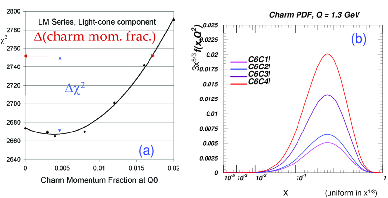
Fig. 3.1.19a shows the overall of the global fit as a function of the size of the input charm degree of freedom of the nucleon at , as measured by the momentum fraction carried by the -quark. We see that, whereas the lowest corresponds to a non-zero charm fraction, the minimum is a very shallow one. By the commonly used tolerance of for an acceptable global fit, this analysis sets an upper limit on the fraction of intrinsic charm at the level of . It is quite interesting that current global QCD analysis can, indeed, place a reasonable upper limit on the charm content of the nucleon.
Fig. 3.1.19b shows the shape of the charm distribution for the series of input functions with increasing amount of charm inside the nucleon in the intrinsic charm scenario. The horizontal axis scale is —intermediate between linear and logarithmic—in order to display both large and small x behaviors clearly. The vertical axis scale is , so that the area under the curves is proportional to the momentum fraction carried by the distribution.
Fig. 3.1.20 shows the shape of charm distributions for the same series as those of the previous plot, but at higher energy scales.
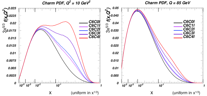
At , we see clearly that has a two-component form: a radiatively generated component peaking at small ; and the evolved intrinsic component at higher . At —around the W/Z mass range, the radiatively generated component is dominant, but the intrinsic component can still be seen. The latter can have physically observable effects on processes that are sensitive to charm in future collider studies, but it would take dedicated efforts to uncover them.
Prospects
The above results represent only the beginning of the exploration of the heavy quark sector of the nucleon structure. They can then help set important benchmarks for new measurements. On one hand, one can map out the range of uncertainties of the predicted cross sections for the proposed measurements. These are expected to be quite wide, given the paucity of existing experimental constraints. On the other hand, by the same global analysis tools, one can assume some measurement goals in terms of hoped for accuracy, and determine how much improvement on our knowledge of the heavy flavor parton distributions can result from such measurements if the goals can be achieved. Such studies would provide valuable input to the planning of the real measurements and the physics analysis of the results.
This effort requires close cooperation between theorists and experimentalists. From the experimental side, it is important to assess the difficulties and the opportunities. The following article [49] summarizes some of the CDF measurements involving heavy quark production in the final state, stating the present status of the analysis, the main sources of systematic errors and possible improvements with larger statistics.
If the course laid out above is actively pursued at Tevatron Run II with concerted effort by experimentalists and theorists, enough real progress might be made to provide valuable input to the execution of Top/Higgs physics studies at the LHC, as well as further improvements on the measurement of heavy quark degrees of freedoms at the LHC itself.
3.2 Some Extrapolations of Tevatron Measurements and the Impact on Heavy Quark PDFs
Contributed by: Campanelli
Most of the measurements at hadron colliders, in particular cross sections, are sensitive to parton distribution functions of the colliding protons. The most uncertain PDF determinations are those referring to heavy quarks, since very few measurements exist and the present estimation are coming from NLO evolutions from the gluon PDF’s.
In the following we summarize some of the CDF measurements involving heavy quark production in the final state, stating the present status of the analysis, the main sources of systematic errors and possible improvements with larger statistics.
When possible, the effect of changing PDF’s has also been included, to be compared to the present and expected uncertainties. The evaluation of the PDF effects follows two different approaches, depending on the analysis. The most used method is to chose a set of PDF’s, and vary by 1 errors the eigenvalues used to express them. Another approach is to consider as an error the maximal variation of the cross section between a given set of PDF’s chosen as standard, and other available sets. Errors obtained using the first method are more rigorous from the statistical point of view, while the second is more conservative.
In general, sources of systematics common to all analyses are the error on luminosity, on the energy scale and on b-tagging. Apart from the luminosity error (that can be reduced using proper normalisation channels), these uncertainties are expected to be reduced with the accumulation of new data. However, this improvement will involve a lot of work to achieve a better knowledge of the detector, and will most likely not scale as fast as the statistical error. Eventually, even if the accumulation of more statistics is the only way to reduce systematic errors, these are most like to end up dominate most of the measurements presented.
Heavy quarks and photons
The present CDF analysis is using data taken with an unbiased photon trigger, with a 25 GeV cut on the transverse photon energy, and no additional requirement on the rest of the event. Offline, the photon is required to pass strong quality requirements, and an hadronic jet with 20 GeV transverse energy, tagged as an heavy flavor. The jet tagging is based on finding a suitable secondary vertex from the tracks in the jet. It has an efficiency of about 40% (jet- dependent) for beauty, few % for charm and about 0.5% for light quarks. However, given the relative abundance of these jets, the tagged sample contains an approximately equal amont of these three categories; to get the cross sections for production of beauty and charm, a fit is performed on the invariant mass of the tracks that constitute the secondary vertex found.
The present CDF analysis uses 67 of data, and an update to higher integrated luminosities is in preparation. The photon energy distribution for selected events is shown in figure 3.2.21. The different corrections for charm and beauty events lead to the cross sections shown on the left and right plots, respectively.

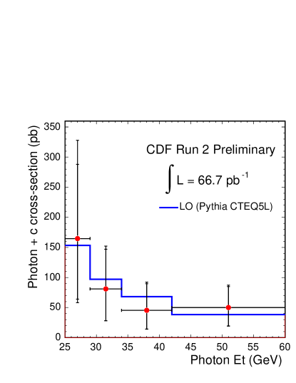
So far statistical error is larger than the systematics, but analyses on datasets about ten times as large as those presented here are almost finished. A table with statistical and systematic errors on the b-photon analysis is shown in 3.2.1; the errors for the c-photon case are very similar in relative importance.
| range (GeV) | 25-29 | 29-34 | 34-42 | 42-60 |
|---|---|---|---|---|
| Tag Efficiency | +1.7-1.3 | +2.6-2.0 | +0.9-0.7 | +1.1-0.9 |
| Photon Id | 0.2 | 0.1 | 0.1 | 0.1 |
| Jet correction | 0.5 | +0.5 | +0.1 | +0.1 |
| Jet energy scale | +3.3-1.4 | +2.2-2.1 | +0.5-0.3 | +0.5-0.4 |
| B jet correction | 0.2 | 0.3 | 0.1 | 0.1 |
| CPR fake estimate | +0.1 | 0.1 | ||
| trigger | +2.5-1.7 | |||
| luminosity | ||||
| 0.3 | 0.5 | 0.2 | 0.2 | |
| Statistical | 11.2 | 17.2 | 6.2 | 7.9 |
| Systematics | +16.4-8.2 | +12.3-10.1 | +6.4-4.4 | +5.0-4.1 |
The dominant systematic errors are the jet energy scale and the tagging efficiency; both of them are expected to decrease with luminosity, albeit not as quick as the statistical error; it is therefore likely that this measurement will start to be systematics dominated. Moreover, while the statistical errors in the various bins are uncorrelated, the effect of a change in PDF’s is likely to be a simultaneous shift of all bins in the same direction, so the biggest obstacle to PDF’s determination will be global effects like enregy scale, -tagging efficiency and luminosity. Although they can be certainly be controlled with a precision at least a factor of 2-3 better than the present analysis, from the numbers in the table it is not likely that their precision can be better than the effect of varying the PDF’s within present limits, indicated as the last source of systematics. This measurement will probably not allow a direct determination of the PDF’s, however it will provade an extremely valid cross-check of the latters, that so far have only been indirectly derived from the gluon distribution. Another experimental approach being pursued by CDF on this measurement is the use of a dataset with a lower threshold on the photon at trigger level (12 GeV), but the requirement for a track with impact parameter measured on-line. This study will allow adding more high-statistics low- bins to the measurement, however the question remains if the trigger efficiencies will be understood at a sufficient level to reach the precision envisaged to observe effects due to PDF’s.
Heavy quarks and bosons
The production of beauty and charm in association with a boson decaying into electrons and muons is presently measured in CDF for an integrated luminosity of about 340 . We require two opposite-charge leptons to lie inside a mass window, and a jet tagged as an heavy quark, with the same -tagging tagging as the previous analysis. The leptonic channel (without -tagging) is used as a normalization channel, to account from trigger and detector effects directly from data. The separate contributions from beauty, charm and light quarks are extracted, similarly to the previous analysis, from a fit to the vertex mass of the tagged jet (figure 3.2.22, left). The distribution of the selected quarks is shown in figure 3.2.22, right. The preliminary measured cross sections and branching fractions have presently a statistical error of about 30%, and a systematic error about half this value.
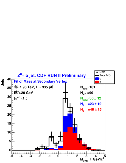
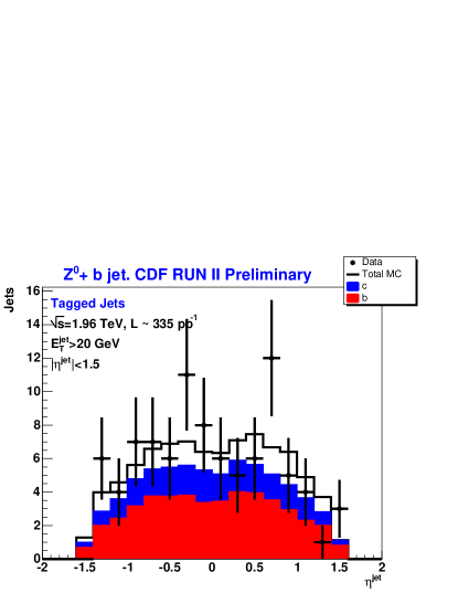
We can assume that systematic errors will end up being around 10%,and that statistical errors of the same order of magnitude will be obtained with data already available. A further improvement towards a total (statistics + systematics) error of the order of 10-15% could be envisaged for the final Tevatron dataset.
Heavy quarks and bosons
The signature of a b quark and a boson is characteristic of single top production, a signal long sought after since Run I. The final state searched for is an electron or muon plus missing energy, compatible with a W bosons, plus at least one b-tagged hadronic jet. The latest CDF publication [50] uses a data sample corresponding to an integrated luminosity of 162 pb-1, and puts a 95% C.L. of 17.8 pb for the combined cross section of s- and t-channel. As expected, from the distribution in figure 3.2.23, most of the observed data comes from QCD production.
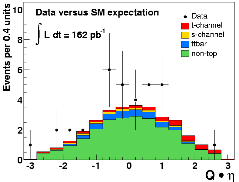
Table 3.2.2 shows the main sources of systematic uncertainty on single top production. The PDF error is the cross section difference between the “standard” set used in the analysis (CTEQ5L) and the one leading to the largest variation (MRST72). Using this conservative method, differences can be relevant even with the present limited statistics. Moreover, since the PDF influence is different for the s- and for the t-channel, the rapidity distribution, shown above, can yield additional information with respect to the simple cross section measurement.
| Source | Syst. error (%) |
|---|---|
| Energy Scale | +0.1-4.3 |
| Initial State Radiation | 1.0 |
| Final State Radiation | 2.6 |
| Generator | 3 |
| Top quark mass | -4.4 |
| Trigger, lepton ID, Lumi | 9.8 |
| 3.8 |
Inclusive cross section
This measurement requires the presence of a tagged hadronic jet in the event, collected with a series of prescaled triggers with cuts on rising values of the jet transverse energy. A vertex mass method is used to extract the fraction, and corrections for the b-tagging efficiency and jet energy scale are applied. This measurement, performed on an integrated luminosity of 300 pb-1 covers a jet range between 38 and 400 GeV, where the cross section spans over six orders of magnitude. The resulting cross section is shwn in figure 3.2.24.
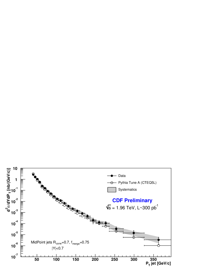
The main systematics for this measurement are summarised in table 3.2.3; since systematics are individually computed for each bin, in the table only an indicative value for the low- and the high- ends of the spectrum are given.
| Source | Syst. low- (%) | Syst. high- (%) |
|---|---|---|
| Energy Scale | +10-8 | +39-22 |
| Energy resolution | 6 | 6 |
| Unfolding | 5 | 15 |
| b fraction | +14-15 | +47-50 |
| b-tagging eff. | 7 | 7 |
| Luminosity | 6 | 6 |
| 7 | 20 |
We see that the jet energy scale and the calculation of the b fraction largely dominate the error, and they increase at high-, where statistics of the control samples is scarcer. More data can certainly improve these errors, possibly by a factor of 2 in the low- and intermediate region, and more in the high-energy region. A global fit of the spectrum, and of the angular distribution will e needed to extract most of the information about PDF’s.
Conclusions
We highlighted some of the production measurements recently performed in CDF, and their sensitivity to PDF’s measurements. With present measurements we are still far from observing effects due to uncertainties in PDF’s in CDF data. A lot of work will be needed to reduce the systematic uncertainties, especially those relative to the jet energy scale and the -tagging efficiency and purity. For doing that, the largest possible control samples are needed, so these measurements will benefit from as much data as possible. Even if they will end up being limited by systematics, the only way to reduce this systematics will be to accumulate more statistics. In any case, even if it will turn out that none of these single measurements will alone be able to constraint present errors on PDF models, they will constitute a fundamental direct cross-check of the validity of these distributions, so far only derived by QCD calculations.
3.3 Issues of QCD Evolution and Mass Thresholds in Variable Flavor Schemes and their Impact on Higgs Production in Association with Heavy Quarks
Contributed by: B. Field, Olness, Smith
We examine some general issues regarding Parton Distribution Functions (PDF’s) involving different numbers of heavy flavors. Specifically we compare the differences and similarities between , , and flavor number scheme PDF’s for lowest order (LO), next-to-leading order (NLO), and next-to-next-to-leading order (NNLO) evolutions. We look at the implications for these different schemes and orders of perturbation expansions, and also study the matching conditions at the threshold. We use the cteq6 data fit as our starting point in comparing the different evolutions.
The LHC will span an unprecedented range of energies and open up new kinematic regions for exploration and discovery. This large energy range poses a theoretical challenge as we encounter multi-scale processes involving many distinct energy/momentum scales. Understanding the data that is to come from the Large Hadron Collider (LHC) in the coming years will require a detailed and precise understanding of parton distribution functions through next-to-next-to-leading order (NNLO).
As we move through these different energy ranges, one can consider implementing PDF’s with varying number of flavors . If our experiments were confined to a limited energy range, a single flavor scheme would be adequate; however, since the energy scales are widely varying, it becomes necessary to use a series of different schemes () to accurately describe the entire energy range. The question of how and where to “join” these schemes also raises significant issues 222The recent paper by Thorne[51] considers some of these issues and choices, particularly the issues that arise at NNLO.. While it is common to join these schemes at an energy scale equal to the quark mass (i.e., ) since the PDF’s will be continuous (but with discontinuous derivatives) at LO and NLO with this matching condition, we see this property is no longer true at NNLO.
Issues of Flavor Schemes
We can illustrate some of these issues by considering the example of Higgs production via b-quarks in the kinematic range where the b-quark mass is too heavy to be ignored, but too light to be decoupled from the hadron dynamics. To work towards a solution which is valid throughout the full energy spectrum, we start by focusing on the asymptotic high and low energy regions (where the issues are simpler), and then try and make these disparate regions match in the (more difficult) intermediate region.
For example, if the characteristic energy range is small compared to the b-quark mass , then the b-quark decouples from the dynamics and does not appear as a partonic constituent of the hadron; that is, and we are working in a flavor scheme. In such a scheme, the Higgs is produced in the process with -pairs in the intermediate state. Calculations in the flavor scheme have the advantage that they do not need to introduce the b-quark PDF. If instead we consider energy scales much larger than the b-quark mass (), then we work in a flavor scheme where the b-quark does appear as a partonic constituent of the hadron []. In this regime, the b-quark mass scale enters as powers of which are resummed via the DGLAP equations. This scheme has the advantage that they involve lower-order Feynman graphs, and the terms are resummed. Ideally, there is an intermediate region where both the 4-flavor and 5-flavor schemes are both a good representation of the physics; in this region we can transition from the low energy 4-flavor scheme to the high energy 5-flavor scheme thereby obtaining a description of the physics which is valid throughout the entire energy range from low to high scales333We label the 4-flavor and 5-flavor schemes as “fixed-flavor-number” (FFN) schemes since the number of partons flavors is fixed. The hybrid scheme which combines these FFS is a “variable-flavor-number” (VFN) scheme since it transitions from a 4-flavor scheme at low energy to a 5-flavor scheme at high energy[42, 52]..
In this report, we will focus on the different PDF’s which result from different orders of evolution (LO, NLO, NNLO) and different numbers of active flavors ().
Generation of PDF Sets
For the purposes of this study, we will start from a given set of PDF’s at an initial scale . We will then evolve the PDF’s from this point and study the effect of the number of active heavy flavors , as well as the order of the evolution: {LO, NLO, NNLO}. No fitting is involved here; the resulting PDF’s are designed to such that they are all related (within their specific -scheme and order of evolution) to be related to the same initial PDF, . In this sense, our comparisons will be focused on comparing schemes and evolution, rather than finding accurate fits to data. Were we able to perform an all-orders calculation, the choice of the number of active heavy flavors would be equivalent; however, since we necessarily must truncate the perturbation expansion at a finite order, there will be differences and some choices may converge better than others.
For our initial PDF, , we chose the cteq6 parametrization as given in Appendix A of Ref. [53]. Using the evolution program described in Ref. [54], we created several PDF tables for our study. Essentially, we explored two-dimensions: 1) the number of active heavy flavors , and 2) the order of the evolution: {LO, NLO, NNLO}; each of these changes effected the resulting PDF. All the sets were defined to be equivalent at the initial scale of GeV. For the set, the charm and bottom quarks are never introduced regardless of the energy scale . The set begins when the charm quark is introduced at GeV. The set begins when the bottom quark is introduced at GeV.
Technical Issues:
Before we proceed to examine the calculations, let’s briefly address two technical issues.
When we evolve the b-quark PDF in the context of the DGLAP evolution equation , we have the option to use splitting kernels which are either mass-dependent [] or mass-independent []. While one might assume that using yields more accurate results, this is not the case. The choice of or is simply a choice of scheme, and both schemes yield identical results up to high-order corrections[55]. For simplicity, it is common to use the mass-independent scheme since the coincide with the kernels.
When the factorization proof of the ACOT scheme was extended to include massive quarks, it was realized that fermion lines with an initial or internal “cut” could be taken as massless[56]. This simplification, referred to as the simplified-ACOT (S-ACOT) scheme, is not an approximation; it is again only a choice of scheme, and both the results of the ACOT and S-ACOT schemes are identical up to high-order corrections[43]. The S-ACOT scheme can lead to significant technical simplifications by allowing us to ignore the heavy quark masses in many of the individual Feynman diagrams. We show how we exploit this feature in the case of NNLO calculation of in the next section.
Consistency Checks
We first recreated the published cteq6 table to check our evolution program and found excellent agreement. The evolution program was also checked against the output described and cataloged in Ref. [57] and was found to be in excellent agreement (generally five decimal places) for all three orders when run with the same inputs444The NNLO results presented here and in Ref. [57] used an approximate form for the three-loop splitting functions since the exact results were not available when the original programs were produced[54]. A comparison of the NNLO splitting functions finds the approximate quark distributions underestimate the exact results by at most a few percent at small x (), and overestimate the gluon distributions by about half a percent for GeV[58]. This accuracy is sufficient for our preliminary study; the evolution program is being updated to include the exact NNLO kernels..
Matching Conditions
A common choice for the matching between and schemes is to perform the transition at . To be specific, let us consider the transition between and flavors at . If we focus on the charm () and gluon () PDF’s, the boundary conditions at NNLO can be written schematically as555Here we use the short-hand notation for the flavor PDF.:
where and . Because the terms vanish when , the above conditions are particularly simple at this point.
An explicit calculation shows that and . Consequently, if we perform the matching at where , we have the continuity condition and . Therefore, the PDF’s will be continuous at LO and NLO.
This is no longer the case at NNLO. Specifically, the coefficients and have been calculated in Ref. [59] and found to be non-zero. Therefore we necessarily will have a discontinuity no matter where we choose the matching between and schemes; is no longer a “special” transition point. This NNLO discontinuity changes the boundary value of the differential equations that govern the evolution of the partons densities, thus changing the distributions at all energy levels; these effects then propagate up to higher scales.
It is interesting to note that there are similar discontinuities in the fragmentation function appearing at NLO. For example the NLO heavy quark fragmentation function first calculated by Nason and Mele[60]
found the coefficient was non-zero. Additionally, we note that is discontinuous across flavor thresholds at order [61]:
Note that the NNLO matching conditions on the running coupling as increases across heavy-flavor flavor thresholds have been calculated in [62, 63] and [64, 65].
Comparison of 3,4, and 5 Flavor Schemes
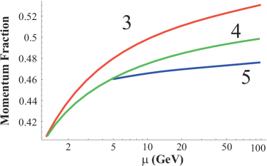
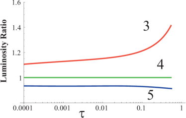
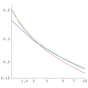
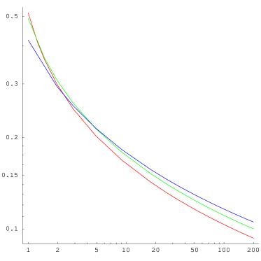
To illustrate how the active number of “heavy” flavors affects the “light” partons, in Fig. 3.3.25a) we show the momentum fraction of the gluon vs. . We have started with a single PDF set at GeV, and evolved from this scale invoking the “heavy” flavor thresholds as appropriate for the specified number of flavors. While all three PDF sets start with the same initial momentum fraction, once we go above the charm threshold ( GeV) the gluon momentum fractions are depleted by the onset of a charm quark density. In a similar fashion, the gluon momentum fraction for is depleted compared to by the onset of a bottom quark density above the bottom threshold ( GeV).
To gauge the effect of the different number of flavors on the cross section, we compute the gluon-gluon luminosity which is defined as . We choose a scale of GeV which is characteristic of a light Higgs. In terms of the luminosity, the cross section is given as with .
To highlight the effect of the different PDF’s, we plot the ratio of the luminosity as compared to the case, c.f., Fig. 3.3.25b). We see that the effects of Fig. 3.3.25a) are effectively squared (as expected—) when examining the thin lines of Fig. 3.3.25b).
However, this is not the entire story. Since we are interested in which is an process, we must also take this factor into account. Therefore we display computed at NLO for as a function of in Fig. 3.3.26. Note at this order, is continuous across flavor boundaries. Fig. 3.3.26 explicitly shows that and . Comparing Figs. 3.3.25 and 3.3.26 we observe that the combination of the and effects tend to compensate each other thereby reducing the difference. While these simple qualitative calculations give us a general idea how the actual cross sections might vary, a full analysis of these effects is required to properly balance all the competing factors. However, there are additional considerations when choosing the active number of flavors, as we will highlight in the next section.
Resummation
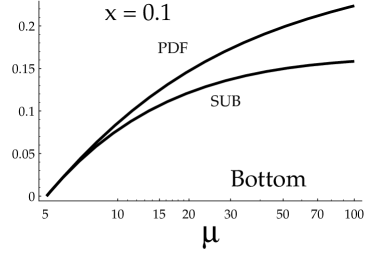
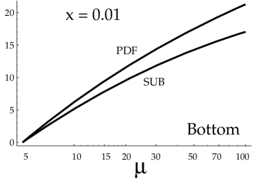
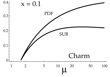
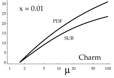
The fundamental difference between the process and the amounts to whether the radiative splittings (e.g., ) are computed by the DGLAP equation as a part of the parton evolution, or whether they are external to the hadron and computed explicitly. In essence, both calculations are represented by the same perturbation theory with two different expansion points; while the full perturbation series will yield identical answers for both expansion points, there will be difference in the truncated series.
To understand source of this difference, we examine the contributions which are resummed into the b-quark PDF by the DGLAP evolution equation, . Solving this equation perturbatively in the region of the b-quark threshold, we obtain . This term simply represents the first-order splitting which is fully contained in the calculation.
In addition to this initial splitting, the DGLAP equation resums an infinite series of such splittings into the non-perturbative evolved PDF, . Both and are shown in Fig. 3.3.27 for two choices of .[66] Near threshold, we expect to be dominated by the single splitting contribution, and this is verified in the figure. In this region, and are comparable, and we expect the 4-flavor calculation should be reliable in this region. As we move to larger scales, we see and begin to diverge at a few times since includes higher-order splitting such as which are not contained in . In this region, we expect the 5-flavor calculation should be most reliable in this region since it resums the iterative splittings. For comparison, and are shown in Fig. 3.3.28 which have similar behavior.
NNLO
The fixed-flavor NLO QCD corrections to charm quark electro-production were calculated in Ref. [67] in the three-flavor scheme. The treatment of the heavy quark as a parton density requires the identification of the large logarithmic terms , which was done in Ref. [59] through next-to-next-leading order (NNLO). Then based on a two-loop analysis of the heavy quark structure functions from an operator point of view, it was shown in Refs. [68], [69] and [70] how to incorporate these large logarithms into charm (and bottom) densities. Two different NNLO variable flavor number schemes were defined in Refs. [71] and [72], where it was shown how they could be matched to the three-flavor scheme at small , the four-flavor scheme at large , and the five-flavor scheme at even larger .
This NNLO analysis yielded two important results. One was the complete set of NNLO matching conditions for massless parton evolution between and flavor schemes. Unlike the LO and NLO case, the NNLO matching conditions are discontinuous at these flavor thresholds. Such matching conditions are necessary for any NNLO calculation at the LHC, and have already been implemented in parton evolution packages by [54], [73].
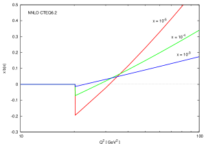
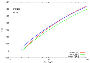
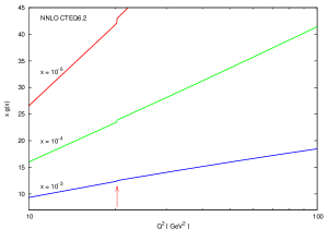
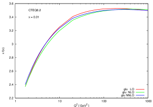
We illustrate this property in Figs. 3.3.29 and 3.3.30. In Fig. 3.3.29, we see that vanishes for ; however, due to the non-vanishing NNLO coefficients, we find is non-zero (and negative) just above the scale. This leads to a discontinuity in the b-quark PDF when making the transition from the to scheme. Additionally, note that the value of the discontinuity is -dependent; hence, there is no simple adjustment that can be made here to restore continuity. We also observe that there is a discontinuity in the gluon PDF across the to transition. While the PDF’s have explicit discontinuities at , the net effect of these NNLO PDF discontinuities will compensate in any (properly calculated) NNLO physical observable such that the final result can only have discontinuities of order .
Finally, we note that the NNLO two-loop calculations above explicitly showed that the heavy quark structure functions in variable flavor approaches are not infrared safe. A precise definition of the heavy-flavor content of the deep inelastic structure function requires one to either define a heavy quark-jet structure function, or introduce a fragmentation function to absorb the uncanceled infrared divergence. In either case, a set of contributions to the inclusive light parton structure functions must be included at NNLO.
Conclusions
While an exact “all-orders” calculation would be independent of the number of active flavors, finite order calculations necessarily will have differences which reflect the higher-order uncalculated terms. To study these effects, we have generated PDFs for flavors using {LO, NLO, NNLO} evolution to quantify the magnitude of these different choices. This work represents an initial step in studying these differences, and understanding the limitations of each scheme.
Acknowledgements
We thank John Collins and Scott Willenbrock for valuable discussions. F.I.O acknowledge the hospitality of Fermilab and BNL, where a portion of this work was performed. This work is supported by the U.S. Department of Energy under grants DE-FG02-97ER41022 and DE-FG03-95ER40908, the Lightner-Sams Foundation, and by the National Science Foundation under grant PHY-0354776.
3.4 LHAPDF: PDF Use from the Tevatron to the LHC
Contributed by: Bourilkov, Group, Whalley
The experimental errors in current and future hadron colliders are expected to decrease to a level that will challenge the uncertainties in theoretical calculations. One important component in the prediction of uncertainties at hadron colliders comes from the Parton Density Functions (PDFs) of the (anti)proton.
The highest energy particle colliders in the world currently, and in the near future, collide hadrons. To make predictions of hadron collisions, the parton cross sections must be folded with the parton density functions:
| (3.4.1) |
with
-
- cross section for the partonic subprocess
-
, - parton momentum fractions,
-
- probability to find a parton with momentum fraction in the (anti)proton.
A long standing problem when performing such calculations is to quantify the uncertainty of the results coming from our limited knowledge of the PDFs. Even if the parton cross section is known very precisely, there may be a sizable error on the hadronic cross section due to the PDF uncertainty. The Tevatron can contribute to PDF knowledge in many ways that will benefit the experiments at the LHC. First, measurements made by the experiments at FNAL will reduce PDF uncertainties by constraining PDF fits. Perhaps more importantly tools and techniques for propagating PDF uncertainty through to physical observables can be improved and tested at the Tevatron.
Next-to-leading order (NLO) is the first order at which the normalization of the hard-scattering cross sections has a reasonable uncertainty. Therefore, this is the first order at which PDF uncertainties are usually applied. To date, all PDF uncertainties have been calculated in the context of NLO global analysis. However, useful information can still be obtained from NLO PDF uncertainties with leading order (LO) calculations and parton shower Monte Carlos [74].
Techniques and tools for calculating PDF uncertainty in the context of LO parton shower Monte Carlos will be the primary topic of this document. Examples are provided employing CTEQ6 [53] error sets from LHAPDF and the parton shower Monte Carlo program PYTHIA [75].
LHAPDF update
Historically, the CERN PDFLIB library [76] has provided a widely used standard FORTRAN interface to PDFs with interpolation grids built into the PDFLIB code itself. However, it was realized that PDFLIB would be increasingly unable to meet the needs of the new generation of PDFs which often involve large numbers of sets (20–40) describing the uncertainties on the individual partons from variations in the fitted parameters. As a consequence of this, at the Les Houches meeting in 2001 [57], the beginnings of a new interface were conceived — the so-called Les Houches Accord PDF (LHAPDF). The LHAGLUE package [77] plus a unique PDF numbering scheme enables LHAPDF to be used in the same way as PDFLIB, without requiring any changes in the PYTHIA or HERWIG codes. The evolution of LHAPDF (and LHAGLUE) is well documented [78, 79].
Recently, LHAPDF has been further improved. With the release of v4.1 in August of 2005 the installation method has been upgraded to the more conventional configure; make; make install. Version 4.2, released in November of 2005, includes the new cteq6AB (variable ) PDF sets. It also includes new modifications by the CTEQ group to other cteq code to improve speed. Some minor bugs were also fixed in this version that affected the a02mnnlo.LHgrid file (previous one was erroneously the same as LO) and SMRSPI code which was wrongly setting usea to zero.
A v5 version, with the addition of the option to store PDFs from multiple sets in memory, has been released. This new functionality speeds up the code by making it possible to store PDF results from many sets while only generating a MC sample once without significant loss of speed.
As a technical check, cross sections have been computed, as well as errors where appropriate, for all PDF sets included in LHAPDF. 10,000 events are generated for each member of a PDF set for both HERWIG [80] and PYTHIA [75], and at both Tevatron and LHC energies. As this study serves simply as a technical check of the interface, no attempt was made to unfold the true PDF error. The maximum Monte Carlo variance (integration error) in our checks is less than 1 percent. This has not been subtracted and will result in an overestimate of the true PDF uncertainty by a factor in our analysis. The results in general show good agreement for most PDFs included in the checks. Overall the consistency is better for Tevatron energies, where we do not have to make large extrapolations to the new energy domain and much broader phase space covered by the LHC.
Two complementary processes are used:
-
•
Drell–Yan Pairs (): the Drell–Yan process is chosen here to probe the functionality of the quark PDFs included in the LHAPDF package.
-
•
Higgs Production: the cross section for probes the gluon PDFs, so this channel is complementary to the case considered above.
PDF uncertainties
As stated above, the need to understand and reduce PDF uncertainties in theoretical predictions for collider physics is of paramount importance. One of the first signs of this necessity was the apparent surplus of high events observed in the inclusive jet cross section in the CDF experiment at FNAL in run I. Subsequent analysis of the PDF uncertainty in this kinematic region indicated that the deviation was within the range of the PDF dominated theoretical uncertainty on the cross section. Indeed, when the full jet data from the Tevatron (including the D0 measurement over the full rapidity range) was included in the global PDF analysis, the enhanced high x gluon preferred by CDF jet data from Run I became the central solution. This was an overwhelming sign that PDF uncertainty needed to be quantified [81]. Below, a short review of one approach to quantify these uncertainties called the Hessian matrix method is given, followed by outlines of two methods used to calculate the PDF uncertainty on physical observables.
Experimental constraints must be incorporated into the uncertainties of parton distribution functions before these uncertainties can be propagated through to predictions of observables. The Hessian Method [82] both constructs a N Eigenvector Basis of PDFs and provides a method from which uncertainties on observables can be calculated. The first step of the Hessian method is to make a fit to data using N free parameters. The global of this fit is minimized yielding a central or best fit parameter set . Next the global is increased to form the Hessian error matrix:
| (3.4.2) |
This matrix can then be diagonalized yielding N (20 for CTEQ6) eigenvectors. Each eigenvector probes a direction in PDF parameter space that is a combination of the 20 free parameters used in the global fit. The largest eigenvalues correspond to the best determined directions and the smallest eigenvalues to the worst determined directions in PDF parameter space. For the CTEQ6 error PDF set, there is a factor of roughly one million between the largest and smallest eigenvectors. The eigenvectors are numbered from highest eigenvalue to lowest eigenvalue. Each N eigenvector direction is then varied up and down within tolerance to obtain 2N new parameter sets, . These parameter sets each correspond to a member of the PDF set, . The PDF library described above, LHAPDF, provides standard access to these PDF sets.
Although the variations applied in the eigenvector directions are symmetric by construction, this is not always the case for the result of these variations when propagated through to an observable. In general the well constrained directions (low eigenvector numbers) tend to have symmetric positive and negative deviations on either side of the central value of the observable (X0). This can not be counted on in the case of the smaller eigenvalues (larger eigenvector numbers). The 2N+1 members of the PDF set provide 2N+1 results for any observable of interest. Two methods for obtaining a set of results are described in detail below. Once results are obtained they can be used to approximate PDF uncertainty through the use of a ’Master Equation’. Although many versions of these equations can be found in the literature, the type which considers maximal positive and negative variations of the physical observable separately is preferred [83]:
| (3.4.3) |
| (3.4.4) |
Other forms of ’Master’ equations with their flaws are summarized:
-
•
This is the original CTEQ ’Master Formula’. It correctly predicts uncertainty on the PDF values since in the PDF basis and are symmetric by construction. However, for physical observables this equation will underestimate the uncertainty if and lie on the same side of . -
•
(,, …)
If and lie on the same side of this equation adds contributions from both in quadrature. NOTE: For symmetric and asymmetric deviations, varies from -
•
positive and negative variations based on eigenvector directions
,
Since the positive and negative directions defined in the PDF eigenvector space are not always related to positive and negative variations on an observable these equations can not be interpreted as positive and negative errors in the general case.
Two main techniques are currently employed to study the effect of PDF uncertainties of physical observables. Both techniques work with the PDF sets derived from the Hessian method.
The ’brute force’ method simply entails running the MC and obtaining the observable of interest for each PDF in the PDF set. This method is robust, and theoretically correct. Unfortunately, it can require very large CPU time since large statistical samples must be generated in order for the PDF uncertainty to be isolated over statistical variations. This method generally is unrealistic when detector simulation is desired.
Because the effect on the uncertainty of the PDF set members is added in quadrature, the uncertainty is often dominated by only a few members of the error set. In this case, a variation of the ’brute force’ method can be applied. Once the eigenvectors that the observable is most sensitive to are determined, MC samples only need to be generated for the members corresponding to the variation of these eigenvalues. This method will always slightly underestimate the true uncertainty.
As mentioned above, often it is not possible to generate the desired MC sample many times in order to obtain the uncertainty on the observable due to the PDF. The ’PDF Weights’ method solves this problem [74]. The idea is that the PDF contribution to Equation 3.4.1 may be factored out. That is, for each event generated with the central PDF from the set, a PDF weight can be stored for each event. The PDF weight technique can be summarized as follows…
-
•
Only one MC sample is generated but 2N (e.g. 40) PDF weights are obtained for
(3.4.5) where
-
•
Only one run, so kinematics do not change and there is no residual statistical variation in uncertainty.
-
•
The observable must be weighted on an event by event basis for each PDF of the set. One can either store a ntuple of weights to be used ’offline’, or fill a set of weighted histograms (one for each PDF in the set).
The benefits of the weighting technique are twofold. First, only one sample of MC must be generated. Second, since the observable for each PDF member is obtained from the same MC sample there is no residual statistical fluctuation in the estimate of the PDF uncertainty. One concern involving this method is that re-weighting events does not correctly modify the Sudakov form factors. However, the difference in this effect due to varying the PDF was shown to be negligible [84]. That is, the initial state parton shower created with the central PDF (CTEQ6.1) also accurately represents the parton shower that would be produced by any other PDF in the error set.
The weighting method is only theoretically correct in the limit that all possible initial states are populated. For this reason, it is important that reasonable statistical samples are generated when using this technique. Any analysis which is sensitive to the extreme tails of distributions should use this method with caution.
There are two options for using the PDF weighting technique. One can either store 2N (e.g. 40 for CTEQ) weights for each event, or store , and and calculate the weights ’offline’. The momentum of the two incoming partons may be obtained from PYTHIA via PARI(33) and PARI(34). Flavour types of the 2 initial partons are stored in and , and the numbering scheme is the same as the one used by LHAPDF, Table 3.4.4, except that the gluon is labeled ’21’ rather than ’0’. The of the interaction is stored in . In theory, this information and access to LHAPDF is all that is needed to use the PDF weights method. This approach has the additional benefit of enabling the ’offline reweighting’ with new PDF sets, which have not been used, or even existed, during the MC generation. We plan to include sample code facilitating the use of PDF weights in future releases of LHAPDF.
| parton | g | d | u | s | c | b | t | ||||||
| n |
Example Studies
The Drell–Yan process is chosen as an almost ideal test case involving quark PDFs for the different flavours.
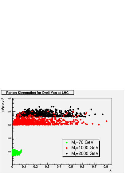
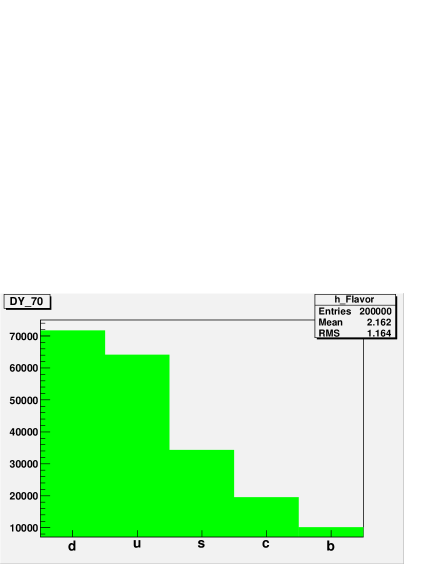
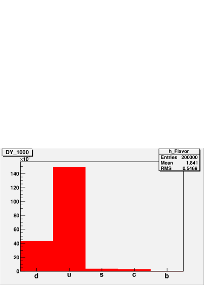
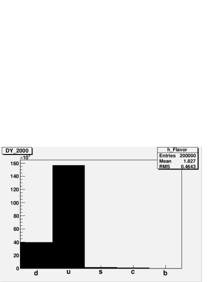
The initial state parton kinematics and flavour contributions are given in Figure 3.4.31 for three regions of invariant mass of the final state lepton pair: GeV. As we can observe, they cover very wide range in X and Q2. It is interesting to note that the flavour composition around the Z peak contains important contributions from five flavours, while at high mass the u and d quarks (in ratio 4:1) dominate almost completely.
Higgs Production in ggH at the LHC is chosen as complementary to the first one and contains only contributions from the gluon PDF. A light Higgs mass of 120 GeV is selected.
As mentioned above, the inclusive jet cross section was one of the first measurements where the need to quantify PDF uncertainty was evident. QCD 2-2 processes are studied for . The kinematic range probed can be seen in Figure 3.4.32.
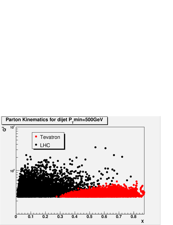
The results for all 3 studies are summarized in Table 3.4.5. The weighting technique produces the same results as the more elaborate ’brute force’ approach for all cases.
| Process (method) | (,) | () | ||||
| DY 70M120 (B.F.) | 1086 | 48 | 42 | |||
| DY 70M120 (W) | 1086 | 48 | 42 | |||
| DY M1000 (B.F.) | 67 | 3.5 | 2.6 | |||
| DY M1000 (W) | 67 | 3.5 | 2.6 | |||
| DY M2000 (B.F.) | 22 | 1.8 | 1.3 | |||
| DY M2000 (W) | 22 | 1.8 | 1.3 | |||
| (B.F.) | 17 | .94 | .68 | |||
| (W) | 17 | .94 | .68 | |||
| DJ500 TeV (B.F.) | 22 | 6.8 | 5.7 | |||
| DJ500 TeV (W) | 22 | 6.8 | 5.7 | |||
| DJ500 LHC (B.F.) | 880 | 63 | 47 | |||
| DJ500 LHC (W) | 880 | 63 | 47 |
Summary
In this contribution, new developments of LHAPDF and consistency checks for all PDF sets are described. The approaches to PDF uncertainty analysis are outlined and the modern method of PDF weighting is described in detail and tested in different channels of current interest. Drell-Yan, gluon fusion to Higgs, and high jet production are studied at the Tevatron and LHC energy scales. The methods are in agreement in all cases. Equations for quantifying PDF uncertainty are discussed and the type which relies on maximal positive and negative variations on the observable is considered superior.
Acknowledgments
The authors would like to thank Joey Huston for encouraging this study. DB wishes to thank the United States National Science Foundation for support from grant NSF 0427110 (UltraLight). CG wishes to thank the US Department of Energy for support from an Outstanding Junior Investigator award under grant DE-FG02-97ER41209. MRW wishes to thank the UK PPARC for support from grant PP/B500590/1.
3.5 fastNLO: Fast pQCD Calculations for PDF Fits
Contributed by Kluge, Rabbertz, Wobisch
We present a method for very fast repeated computations of higher-order
cross sections in hadron-induced processes
for arbitrary parton density functions.
A full implementation of the method
for computations of jet cross sections
in Deep-Inelastic Scattering and in Hadron-Hadron Collisions
is offered by the “fastNLO” project.
A web-interface for online calculations and user code
can be found at
http://hepforge.cedar.ac.uk/fastnlo/.
The aim of the ”fastNLO” project is to make the inclusion of jet data into global fits of parton density functions (PDFs) feasible. Due to the prohibitive computing time required for the jet cross sections using standard calculation techniques, jet data have either been omitted in these fits completely or they were included using a simple approximation. The fastNLO project implements a method that offers exact and very fast pQCD calculations for a large number of jet data sets allowing to take full advantage of their direct sensitivity to the gluon density in the proton in future PDF fits. This includes Tevatron jet data beyond the inclusive jet cross section and also HERA jet data which have been used to determine the proton’s gluon density [85, 86, 87, 88], but which are ignored in current PDF fits [89, 90, 53].
Cross Sections in Perturbative QCD
Perturbative QCD predictions for observables in hadron-induced processes depend on the strong coupling constant and on the PDFs of the hadron(s). Any cross section in hadron-hadron collisions can be written as the convolution of the strong coupling constant in order , the perturbative coefficient for the partonic subprocess , and the corresponding linear combination of PDFs from the two hadrons which is a function of the fractional hadron momenta carried by the partons
| (3.5.6) |
The PDFs and also depend on the factorization and the renormalization scales , respectively, as does the perturbative prediction for the cross section in finite order . An iterative PDF fitting procedure using exact NLO calculations for jet data, based on Monte-Carlo integrations of (3.5.6), is too time-consuming. Only an approximation of (3.5.6) is, therefore, currently being used in global PDF fits.
A Simple Approach

The “-factor approximation” as used in [90, 53] parameterizes higher-order corrections for each bin of the observable by a factor computed from the contributions with () and () for a fixed PDF, averaged over all subprocesses . In the iterative fitting procedure only the LO cross section is computed and multiplied with to obtain an estimate of the NLO cross section. This procedure does not take into account that different partonic subprocesses can have largely different higher-order corrections. Fig. 3.5.33 shows that the -factors for quark-only and gluon-only induced subprocesses can differ by more than from the average. The is therefore minimized under an incorrect assumption of the true PDF dependence of the cross section. Further limitations of this approach are:
-
•
Even the LO Monte-Carlo integration of (3.5.6) is a trade-off between speed and precision. With finite statistical errors, however, theory predictions are not ideally smooth functions of the fit parameters. This contributes to numerical noise in the calculations [91] distorting the contour during the PDF error analysis, especially for fit parameters with small errors.
-
•
The procedure can only be used for observables for which LO calculations are fast. Currently, this prevents the global PDF analyses from using Tevatron dijet data and DIS jet data.
In a time when phenomenology is aiming towards NNLO precision [89, 90], the -factor approximation is clearly not satisfying concerning both its limitation in precision and its restrictions concerning data sets.
The fastNLO Solution


A better solution is implemented in the fastNLO project. The basic idea is to transform the convolution in (3.5.6) into the factorized expression (3.5.9). Many proposals for this have been made in the past, originally related to solving the DGLAP parton evolution equations [92] and later to computing of jet cross sections [93, 94, 95, 96, 97]. The fastNLO method is an extension of the concepts developed for DIS jet production [93, 96] which have been applied at HERA to determine the gluon density in the proton from DIS jet data [85]. Starting from (3.5.6) for the following discussion the renormalization scale is set equal to the factorization scale (). The extension to is, however, trivial. The dependence of the PDFs and the scale dependence of and the PDFs can be approximated using an interpolation between sets of fixed values and ()
| (3.5.7) | |||||
where and are interpolation functions for the and the dependence, respectively. All information of the perturbatively calculable piece (including phase space restrictions, jet definition, etc. but excluding and the PDFs) is fully contained in the quantity
| (3.5.8) |
In the final prediction for the cross section the convolution in (3.5.6) is then reduced to a simple product
| (3.5.9) |
The time-consuming step involving the calculation of the universal (PDF and independent) is therefore factorized and needs to be done only once. Any further calculation of the pQCD prediction for arbitrary PDFs and values can later be done very fast by computing the simple sum of products in (3.5.9). While the extension of the method from one initial-state hadron [96] to two hadrons was conceptually trivial, the case of two hadrons requires additional efforts to improve the efficiency and precision of the interpolation. Both, the efficiency and the precision, are directly related to the choices of the points , and the interpolation functions , . The implementation in fastNLO achieves a precision of better than for and . Computation times for cross sections in fastNLO are roughly 40-200 s per order (depending on ). Further details are given in Ref [98].
Results
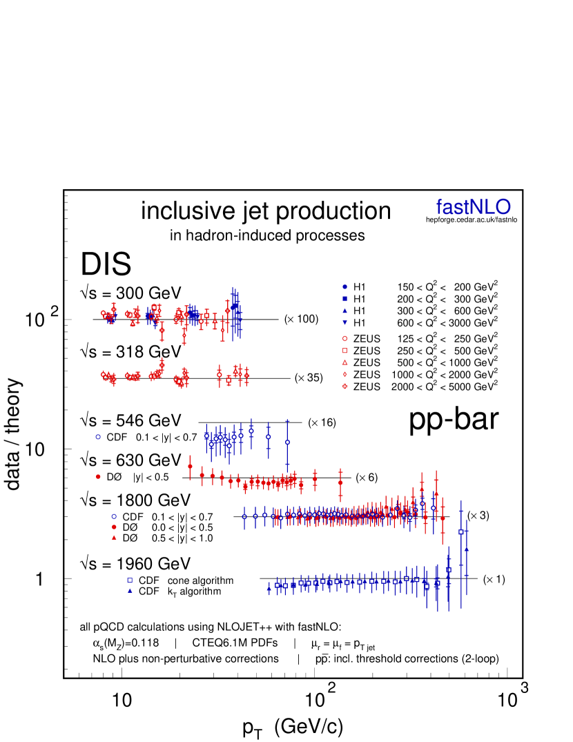
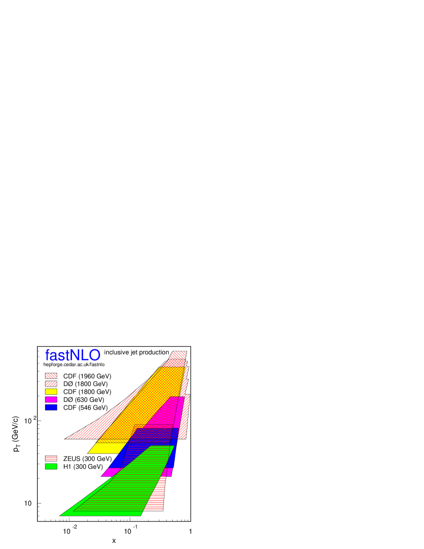
Calculations by fastNLO are available at http://hepforge.cedar.ac.uk/fastnlo for a large set of (published, ongoing, or planned) jet cross section measurements at HERA, RHIC, the Tevatron, and the LHC (either online or as computer code for inclusion in PDF fits). Some fastNLO results for the inclusive jet cross section in different reactions are shown in this section. The contributions from different partonic subprocesses to the central inclusive jet cross section are compared in Fig. 3.5.34 for different colliders: For collisions at RHIC and the LHC, and for scattering at Tevatron Run II energies. It is seen that the quark-induced subprocesses are dominated by the valence quarks: In proton-proton collisions (RHIC, LHC) the quark-quark subprocesses (4,5) give much larger contributions than the quark-antiquark subprocesses (6,7) while exactly the opposite is true for proton-antiproton collisions at the Tevatron. The contribution from gluon-induced subprocesses is significant at all colliders over the whole ranges. It is interesting to note that at fixed the gluon contributions are largest at RHIC. Here, the jet cross section at still receives contributions from gluon-induced subprocesses, as compared to only at the Tevatron or at the LHC. As shown in Fig. 3.5.35, this results in much larger PDF uncertainties for the high inclusive jet cross section at RHIC, as compared to the Tevatron and the LHC for which PDF uncertainties are roughly of the same size (at the same ). This indicates that the PDF sensitivity at the same is about the same at the Tevatron and at the LHC, while it is much higher at RHIC.
An overview over published measurements of the inclusive jet cross section in different reactions and at different center-of-mass energies is given in Fig. 3.5.36. The results are shown as ratios of data over theory. The theory calculations include the best available perturbative predictions (NLO for DIS data and NLO + threshold corrections for data) which have been corrected for non-perturbative effects. Over the whole phase space of GeV jet data in DIS and collisions are well-described by the theory predictions using CTEQ6.1M PDFs [53]. The phase space in and covered by these measurements is shown in Fig. 3.5.37, demonstrating what can be gained by using fastNLO to include these data sets in future PDF fits. A first study using fastNLO on the future potential of LHC jet data has been published in Ref. [102].
4 Event Generator Tuning
4.1 Dijet Azimuthal Decorrelations and Monte Carlo Tuning
Contributed by Begel, Wobisch, Zielinski
Using a recent DØ measurement of correlations in the
dijet azimuthal angle in collisions,
we investigate the description of data
by Monte Carlo event generators.
We analyze the impact of various phenomenological parameters
employed in the generators and demonstrate that the data can
unambiguously constrain the description of Initial State Radiation
(ISR) in PYTHIA.
Finally, we use the next-to-leading order (NLO) pQCD extrapolation
to evaluate the description of QCD radiation effects by
the Monte Carlo tools at the LHC energy.
The proper description of multi-parton radiation is crucial for a wide range of precision measurements as well as for searches for new physical phenomena at the LHC. Thus, it is essential that the Monte Carlo tools employed in data analyses accurately describe the observed aspects of such radiation. While the Monte Carlo generators have been tuned using selected Tevatron and lower energy data, it is interesting to inquire to what extent such tuning will be valid also at the LHC. In particular, the PYTHIA Monte Carlo [103] has been tuned to describe the underlying event in hadron collisions at around TeV [104, 105]. This tuning involved adjusting parameters for (“soft”) physics processes at small transverse momentum, , (hadronization, underlying event) as well as parameters for high (“hard”) physics processes, like parton showering. A significant correlation between the parameters for the soft and the hard contributions was noticed, and the resulting tunes represented different parameter sets which all gave a good description of the underlying-event data [106, 107].
In this paper we study a recent measurement from the DØ collaboration, which allows to isolate the effects of hard physics processes. The DØ collaboration has measured distributions of the azimuthal difference between the two jets with largest in an event [108]. This observable provides an effective probe of radiation effects; consequently, the DØ measurement adds independent information to that included in the previous tunes, and constrains the effects from high initial-state radiation (ISR) unambiguously.
In the following, we compare the data to predictions from Monte Carlo event generators, and investigate the sensitivity of their phenomenological parameters. Finally, we use next-to-leading order (NLO) perturbative QCD (pQCD) predictions to demonstrate that the tuning is successfully transferred to LHC energies.
The Physics of Decorrelations
Dijet azimuthal decorrelations in hadron-hadron collisions are sensitive to different physics processes in different regions of the azimuthal angle between the two leading jets . At Born-level dijet events have two jets with equal with respect to the beam axis and their azimuthal angles are correlated such that . Any deviation from is caused by additional radiation in the event which is not clustered into the two highest jets. Radiation with small will change by a smaller amount, while hard radiation (with high ) can reduce significantly, as illustrated in Fig. 4.1.38. The distribution therefore allows to study the continuous transition from soft (non-perturbative) to hard (perturbative) QCD processes, based on a single observable. The QCD predictions for the different contributions are determined as follows:
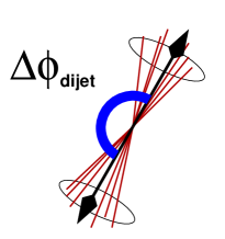
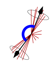
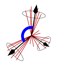
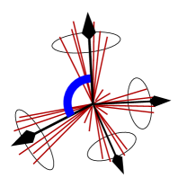
- •
-
•
soft perturbative processes
Fixed-order calculations fail in phase space regions which are dominated by soft multi-parton emissions. In these regions contributions from logarithmic terms are enhanced and need to be resummed to all orders of . Methods for the automated resummation of certain classes of observables in hadron-hadron collisions have recently become available [109, 35]. The distribution is, however, not a “global” observable 666An observable is called “global” when it is sensitive to all particles in the event. The distribution is, however, not sensitive to the particles inside the jets. (as defined in [35]). Therefore these automated resummation methods can not be applied.
An alternative description of multi-parton emissions is given in parton cascade models (parton shower or dipole cascade). These are implemented in Monte Carlo event generators like PYTHIA or HERWIG [80], where they are matched to the Born-level matrix elements. -
•
non-perturbative processes
Processes like hadronization and activity related to the beam remnants (“underlying event”) can not be computed from first principles. Phenomenological models for these processes, matched to the parton cascade models, are used in the Monte Carlo event generators.
Distributions of in Data and Monte Carlo
The experimental observable has been defined as the differential dijet cross section in , normalized by the dijet cross section integrated over in the same phase space: [108]. In this ratio theoretical and experimental uncertainties are reduced. Jets have been defined using an iterative seed-based cone algorithm (including mid-points) [110] with radius at parton, particle, and experimental levels. Four analysis regions have been defined based on the jet with largest in an event (). The second leading- jet in each event is required to have GeV and both jets have central rapidities with .

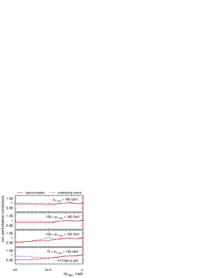
The data are compared to predictions from the PYTHIA and HERWIG generators in Fig. 4.1.39 (left). The observed spectra are strongly peaked at and the peaks are narrower at larger values of . The predictions of the Monte Carlo event generators have been obtained using the respective default settings, unless stated otherwise. The generators are using the cteq6l parton density functions (PDF’s). The values in the generators are adjusted such that the resulting value of is consistent with the world average and with the value that was used in the CTEQ6 PDF fit [53]. Consistent with the procedure in the PDF fit we are using the 2-loop solution for the renormalization group equation. This is the default in HERWIG, but needs to be set in PYTHIA using the switch MSTP(2)=2. Below, these settings will be referred to as the “default” settings.
The default HERWIG (version 6.505) gives a good description of the data over the whole range in all regions. It is slightly below the data around and slightly narrower peaked at . The default version of PYTHIA (version 6.225) does not describe the data. The spectrum is much steeper over the whole range, independent of . These deviations will be investigated in the following.
Non-Perturbative Contributions
Before we investigate the contributions from perturbative QCD processes we study the sensitivity of the distribution to non-perturbative contributions, stemming from the hadronization process or the underlying event.
Fig. 4.1.39 (right, dashed line) shows the underlying event correction, defined as the ratio of the default PYTHIA (including underlying event) and PYTHIA with the underlying event switched off by MSTP(81)=0. It is apparent that the effects from underlying event are below four percent.
The hadronization corrections are defined as the ratio of the observable, on the level of partons (from the parton shower) and on the level of stable particles. Fig. 4.1.39 (right, solid line) shows that these corrections are below 2-5% over the whole range.
We conclude that the distribution is not sensitive to non-perturbative effects and these can not explain the deviations between PYTHIA and the data. Hence we do not attempt to tune the PYTHIA parameters for the hadronization or the underlying event models. We also can neglect the non-perturbative effects when comparing to the purely perturbative NLO QCD predictions.


Parameter Tuning
To investigate the possibilities of tuning PYTHIA we first focus on the impact of the ISR parton shower. PYTHIA contains various parameters by which the ISR shower can be adjusted. The maximum allowed , produced by the ISR shower is limited by the upper cut-off on the parton virtuality. This cut-off is controlled by the product of the parameter PARP(67) and the hard scattering scale squared (which is equal to for massless partons). Increasing this cut-off by varying PARP(67) from its default of 1.0 to 4.0 leads to significant changes of the PYTHIA prediction for . Fig. 4.1.40 shows comparisons of PYTHIA and HERWIG to data over the whole range (left) and in greater detail in the region (right). The increased value of PARP(67) in PYTHIA increases the tail of the distribution strongly, especially at lowest . At large , however, this parameter has not enough effect to bring PYTHIA close to the data. The best description at low is obtained for PARP(67) = 2.5 (referred to as “TeV-tuned” in the following) as shown in Fig. 4.1.43.


In addition, we have tested the impact of other ISR-related parameters in PYTHIA. These are the scale factor () for the renormalization scale for in the ISR shower, PARP(64), and the primordial of partons in the proton: the central value of the gaussian distribution, given by PARP(91), and the upper cut-off, given by PARP(93). We have lowered the factor for the renormalization scale from its default of one to PARP(64)=0.5 which increases the value of . We have alternatively increased the primordial from 1 GeV to 4 GeV, PARP(91)=4.0, and the upper cut-off of the gaussian distribution from 5 GeV to 8 GeV, PARP(93)=8.0. None of these parameter variations has an appreciable effect on the region at low . The effects at large are shown in Fig. 4.1.41 (left). It is clearly visible that they are very small. While the scale factor has almost no influence, there is some small change for the increased primordial which manifests itself only very close to the peak region and only at lower values of .
We have also studied the sensitivity of parameters for the final-state radiation (FSR) parton shower. The maximum of partons from FSR is controlled by the parameter PARP(71) in the same way that PARP(67) controls the maximum from ISR. We have increased PARP(71) from its default value of to . The result is shown in Fig. 4.1.41 (right) and compared to default PYTHIA and to HERWIG. It is seen that the increased in the FSR shower leads only to small changes in the range , decreasing towards higher .
In conclusion, PARP(67) is the only parameter we have found in PYTHIA that has a significant impact on the distribution. While it is not sufficient for a perfect tuning of PYTHIA to data, this observation can be used for an unambiguous determination of the optimal value of this parameter.
Matched Monte Carlo Predictions


Fixed-order matrix-element event generators are used extensively in studies of top and Higgs production. Multi-jet configurations are produced by incorporating high-order tree-level pQCD diagrams with phenomenological parton-shower models such as those from PYTHIA or HERWIG. Verification of their performance using high-statistics QCD processes is of clear interest for applications that require accurate descriptions of processes with several jets. Some of these calculations have prescriptions to avoid double-counting contributions with equivalent phase-space configurations [111, 112]. distributions offer an interesting avenue for testing the smoothness of matching between matrix-element and parton-shower contributions as the average jet multiplicity varies across the range.
ALPGEN [113] uses the MLM matching prescription which rejects events that have reconstructed parton-shower jets that do not overlap with generated partons, thus excluding those events where the jets arose from the parton-shower mechanism. (The highest multiplicity bin includes these extra jets.) Samples with different jet multiplicities are then combined together according to the MLM scheme into an inclusive sample that can be compared to data. Fig. 4.1.42 (left) shows an example of this scheme for multi-jet production. Samples for , , , jet production were combined using the MLM scheme. Individually, none of the contributions compares favorably with the data. However, the combined ALPGEN calculation agrees reasonably well with the data. This result does not depend on the details of the parton-shower model (Fig. 4.1.42 right).
SHERPA [114], another tree-level pQCD event generator, uses the CKKW [115] matching scheme to produce multi-jet events. Here, the parton-shower progression is pruned so that only allowable configurations are produced. SHERPA uses its own parton-shower model; it does not use either PYTHIA or HERWIG. Fig. 4.1.43 shows the results from SHERPA for multi-jet production compared to the DØ data and to the results from HERWIG and the TeV-tuned PYTHIA. The results from SHERPA provide a good description of the data.
Perturbative QCD Predictions
The distributions can be directly employed to test the purely perturbative QCD predictions since non-perturbative corrections can be safely neglected. Fig. 4.1.44 (left) shows the comparison of pQCD calculations obtained using the parton-level event generator nlojet++ [100, 99] and the cteq6.1m PDF’s [53] and data. The integrated dijet cross section and the differential dijet cross section in are computed separately in their respective LO and NLO. In all cases the renormalization and factorization scales are set to .
The leading-order calculation clearly has a limited applicability. Due to the limited phase space for three-parton final states it does not cover the region , and towards it becomes divergent. NLO pQCD provides a good description of the data over most of the range of . Only for the NLO prediction is insufficient, and a resummed calculation is required. It would be of great interest to test the resummation techniques against the data when a resummed result becomes available.


Predictions for the LHC
Having validated the veracity of the NLO calculation for Tevatron data at TeV, we expect it to provide a reliable extrapolation of predictions to the LHC energy of TeV for collisions. To obtain predictions for the LHC, we selected thresholds of 180, 500 and 1200 GeV. The second leading- jet in each event is required to have GeV and both jets have central rapidities with . For these choices, the distributions span a similar range of values as observed at the Tevatron (see Fig. 4.1.44, right).
Summary and Outlook
We conclude that the recent DØ measurement of dijet azimuthal decorrelations unambiguously constrains the ISR parton shower parameters in PYTHIA. While the default parameters produce insufficient levels of ISR with high , a popular tune (tune A which uses PARP(67)=4.0 [106, 107]) predicts too much ISR. Our findings provide additional information for PYTHIA tuning efforts which so far have been based primarily on soft physics in the underlying event. The re-tuned PYTHIA (with PARP(67)=2.5) gives a good description of the DØ data for and it also agrees well with NLO pQCD predictions for this observable. Extrapolated to LHC energies, the agreement of the re-tuned PYTHIA with NLO is preserved. It is encouraging that Monte Carlo tuning to Tevatron data works well also at LHC energies, judging from the comparison to NLO pQCD.
We believe that it will be worthwhile to investigate the distributions at the LHC. They can provide an early test of pQCD and Monte Carlo descriptions of multi-jet processes. This is crucial for the understanding of backgrounds affecting discovery searches. The required dijet data will be accumulated rapidly and with virtually no background. The reduced sensitivity of the measurement to the jet energy calibration, normalization and pileup effects promises to provide insights into the QCD radiation issues at LHC before other multi-jet processes can be measured with sufficient precision.
Thus, the predictions from the TeV-tuned Monte Carlos and NLO pQCD for distributions can and should be verified quickly with the first LHC physics-quality data. Similarly, the expectations from the new Monte Carlo systems, like ALPGEN and SHERPA, currently under development to be among the primary Monte Carlo tools at the LHC, can be verified with early data. In particular, distributions offer an interesting ground for testing the smoothness of matching between Matrix Element and Parton Shower contributions as the jet multiplicity varies across the range. These issues have only begun to be investigated using the Tevatron data [116].
4.2 Tevatron Run 2 Monte-Carlo Tunes
Contributed by: R. Field
Several Tevatron Run 2 PYTHIA 6.2 tunes (with multiple parton interactions) are presented and compared
with HERWIG (without multiple parton interactions) and with the ATLAS PYTHIA tune (with multiple
parton interactions). Predictions are made for the “underlying event” in high jet production and in
Drell-Yan lepton-pair production at the Tevatron and the LHC.
In order to find “new” physics at a hadron-hadron collider it is essential to have Monte-Carlo models that simulate accurately the “ordinary” QCD hard-scattering events. To do this one must not only have a good model of the hard scattering part of the process, but also of the beam-beam remnants and the multiple parton interactions. The “underlying event” is an unavoidable background to most collider observables and a good understanding of it will lead to more precise measurements at the Tevatron and the LHC. Fig. 4.2.46 illustrates the way QCD Monte-Carlo models simulate a proton-antiproton collision in which a “hard” -to- parton scattering with transverse momentum, , has occurred [103, 80]. The “hard scattering” component of the event consists of particles that result from the hadronization of the two outgoing partons (i.e., the initial two “jets”) plus the particles that arise from initial and final state radiation (i.e., multijets). The “underlying event” consists of particles that arise from the “beam-beam remnants” and from multiple parton interactions (MPI). Of course, in a given event it is not possible to uniquely determine the origin of the outgoing particles and whatever observable one chooses to study inevitably receives contributions from both the hard component and the underlying event. In studying observables that are sensitive to the underlying event one learns not only about the beam-beam remnants and multiple parton interactions, but also about hadronization and initial and final state radiation.

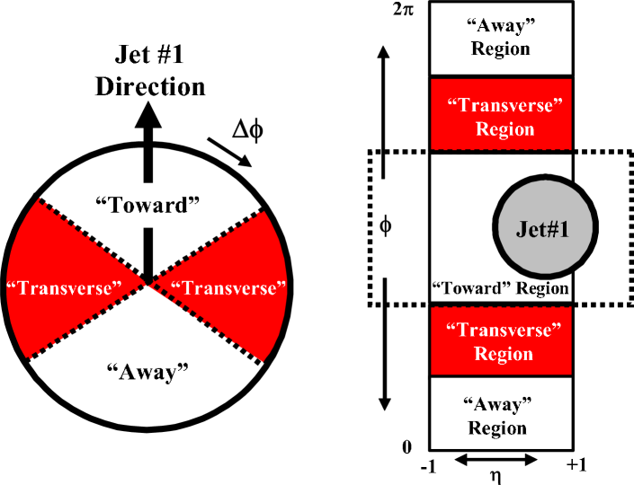
In Run2, we are working to understand and model the “underlying event” at the Tevatron. We use the topological structure of hadron-hadron collisions to study the underlying event [104, 117, 25]. The direction of the leading calorimeter jet is used to isolate regions of - space that are sensitive to the underlying event. As illustrated in Fig. 4.2.47, the direction of the leading jet, jet#, is used to define correlations in the azimuthal angle, . The angle is the relative azimuthal angle between a charged particle and the direction of jet#. The “transverse” region is almost perpendicular to the plane of the hard -to- scattering and is therefore very sensitive to the underlying event. Furthermore, we consider two classes of events. We refer to events in which there are no restrictions placed on the second and third highest jets (jet# and jet#) as “leading jet” events. Events with at least two jets with where the leading two jets are nearly “back-to-back” () with and are referred to as “back-to-back” events. “Back-to-back” events are a subset of the “leading jet” events. The idea here is to suppress hard initial and final-state radiation thus increasing the sensitivity of the “transverse” region to the “beam-beam remnants” and the multiple parton scattering component of the underlying event.
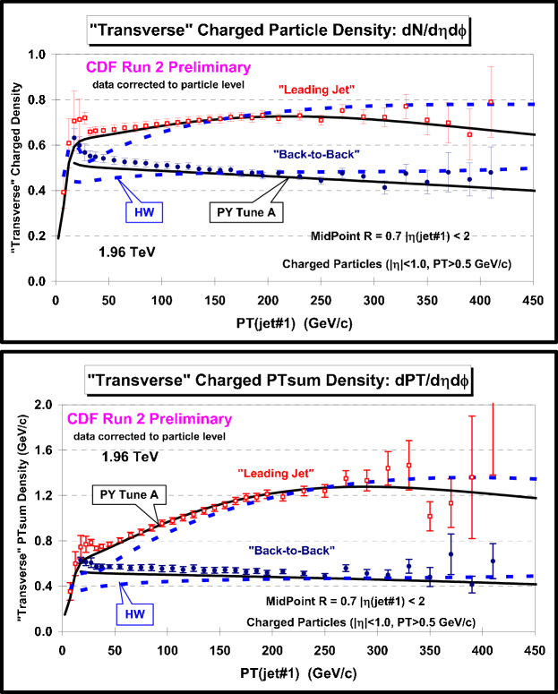
Fig. 4.2.48 compares the data on the density of charged particles and the charged PTsum density in the “transverse” region for “leading jet” and “back-to-back” events with PYTHIA Tune A (with multiple parton interactions) and HERWIG (without multiple parton interactions). As expected, the “leading jet” and “back-to-back” events behave quite differently. For the “leading jet” case the densities rise with increasing , while for the “back-to-back” case they fall slightly with increasing . The rise in the “leading jet” case is, of course, due to hard initial and final-state radiation, which has been suppressed in the “back-to-back” events. The “back-to-back” events allow for a more close look at the “beam-beam remnants” and multiple parton scattering component of the underlying event and PYTHIA Tune A does a better job describing the data than HERWIG. PYTHIA Tune A was determined by fitting the CDF Run 1 “underlying event” data [107].
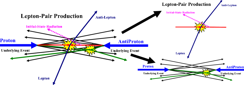
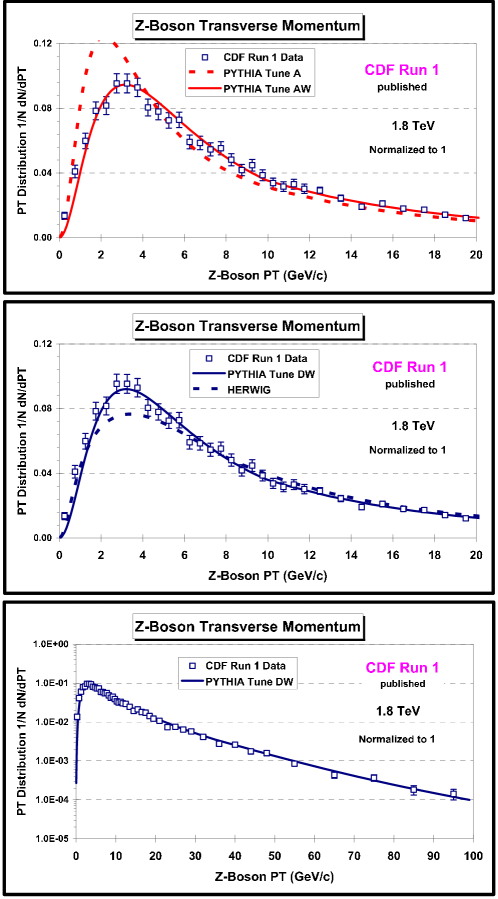
| Parameter | A | AW | DW | DWT | BW | ATLAS | QW |
|---|---|---|---|---|---|---|---|
| CTEQ | 5L | 5L | 5L | 5L | 5L | 5L | 6.1 |
| MSTP(81) | |||||||
| MSTP(82) | |||||||
| PARP(82) | |||||||
| PARP(83) | |||||||
| PARP(84) | |||||||
| PARP(85) | |||||||
| PARP(86) | |||||||
| PARP(89) | |||||||
| PARP(90) | |||||||
| PARP(62) | |||||||
| PARP(64) | |||||||
| PARP(67) | |||||||
| MSTP(91) | |||||||
| PARP(91) | |||||||
| PARP(93) |
| Tune | at | at |
|---|---|---|
| A,AW | mb | mb |
| DW | mb | mb |
| DWT | mb | mb |
| BW | mb | mb |
| QW | mb | mb |
| ATLAS | mb | mb |
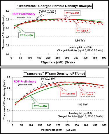
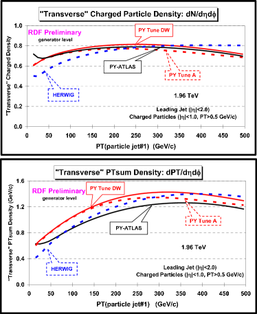
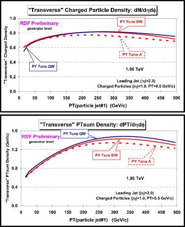
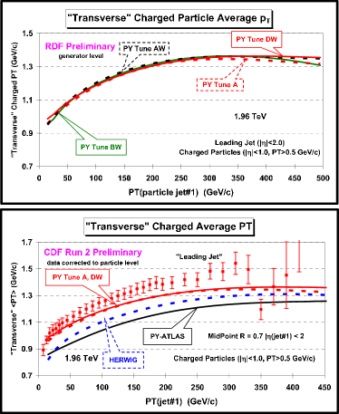
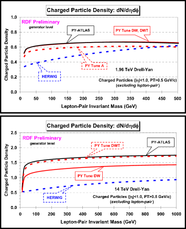
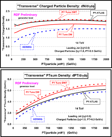
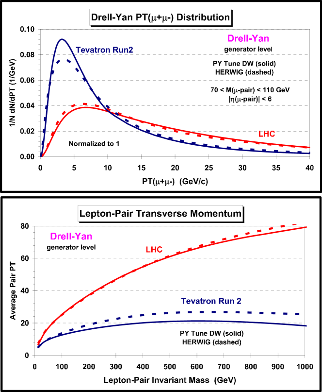
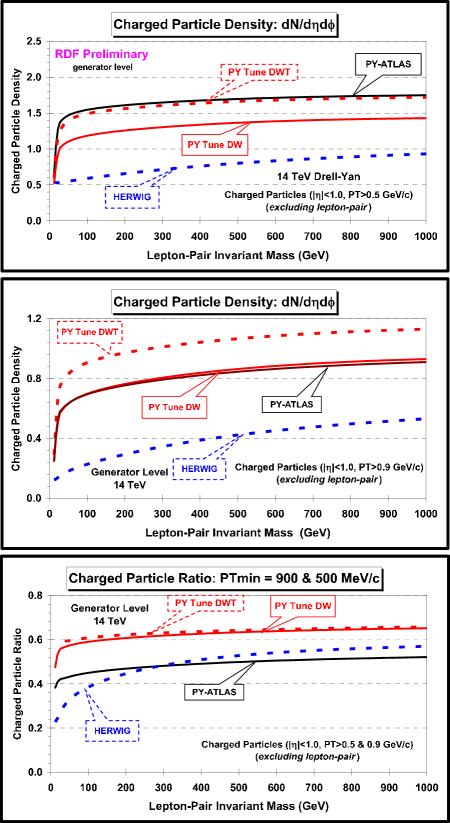
As illustrated in Fig. 4.2.49, Drell-Yan lepton-pair production provides an excellent place to study the underlying event. Here one studies the outgoing charged particles (excluding the lepton pair) as a function of the lepton-pair invariant mass. After removing the lepton-pair everything else results from the beam-beam remnants, multiple parton interactions, and initial-state radiation. Unlike high jet production (Fig. 1) for lepton-pair production there is no final-state gluon radiation.
Fig. 4.2.50 shows that PYTHIA Tune A does not fit the CDF Run 1 -boson distribution [118]. PYTHIA Tune A was determined by fitting the Run 1 “underlying event” data and, at that time, we did not consider the -boson data. PYTHIA Tune AW fits the Z-boson distribution as well as the “underlying event” at the Tevatron 777The values of PARP(62), PARP(64), and PARP(91) were determined by CDF Electroweak Group. The W in Tune AW, BW, DW, DWT, QW stands for Willis. I combined the Willis tune with Tune A, etc. PYTHIA Tune DW is very similar to Tune AW except PARP(67) = 2.5, which is the preferred value determined by DØ in fitting their dijet distribution [119]. HERWIG does a fairly good job fitting the -boson distribution without additional tuning, but does not fit the CDF “underlying event” data.
Table 4.2.6 shows the parameters for several PYTHIA tunes. Tune BW is a tune with . Tune DW and Tune DWT are identical at , but Tune DW and DWT extrapolate differently to the LHC. Tune DWT uses the ATLAS energy dependence, , while Tune DW uses the Tune A value of . The ATLAS Tune is the default tune currently used by ATLAS at the LHC. All the tunes except Tune QW use CTEQ5L. Tune QW uses CTEQ6.1 which is a next-to-leading order structure function. However, Tune QW uses leading order QCD coupling, , with . Note that Tune QW has a much smaller value of (i.e., the MPI cut-off). This is due to the change in the low x gluon distribution in going from CTEQ5L to CTEQ6.1. Table 4.2.7 shows the computed value of the multiple parton scattering cross section for the various tunes. The multiple parton scattering cross section (divided by the total inelastic cross section) determines the average number of multiple parton collisions per event.
As can be seen in Figs. 4.2.51 and 4.2.52(a), PYTHIA Tune A, AW, DW, DWT, and QW have been adjusted to give similar results for the charged particle density and the PTsum density in the “transverse” region with and for “leading jet” events at . PYTHIA Tune A fits the CDF Run 2 “underlying event” data for “leading jet” events and Tune AW, BW, DW, and QW roughly agree with Tune A. Fig. 4.2.52(b) shows that PYTHIA Tune A, Tune DW, and the ATLAS PYTHIA Tune predict about the same density of charged particles in the “transverse” region with for “leading jet” events at the Tevatron. However, the ATLAS Tune has a much softer distribution of charged particles resulting in a much smaller average per particles. Fig. 4.2.52(b) shows that the softer distribution of the ATLAS Tune does not agree with the CDF data.
The predictions of PYTHIA Tune A, Tune DW, Tune DWT, HERWIG, and the ATLAS PYTHIA Tune for the density of charged particles with and for Drell-Yan lepton-pair production at and are shown in Fig. 4.2.53(a). The ATLAS Tune and Tune DW predict about the same charged particle density with at the Tevatron, and the ATLAS Tune and Tune DWT predict about the same charged particle density with at the LHC. However, the ATLAS Tune has a much softer distribution of particles, both at the Tevatron and the LHC. We are working to compare the CDF Run 2 data on Drell-Yan production with the QCD Monte-Carlo models and hope to have results soon.
Fig. 4.2.53(b) shows the predictions of PYTHIA Tune DW, Tune DWT, HERWIG, and the ATLAS Tune for the density of charged particles and the PTsum density in the “transverse” region for “leading jet” production at the LHC. The PYTHIA Tunes (with multiple parton interactions) predict a large increase in the charged particle density in going from the Tevatron (Fig. 4.2.51) to the LHC (Fig. 4.2.53(b)). HERWIG (without multiple parton interactions) does not increase as much. PYTHIA Tune DWT and the ATLAS Tune both predict about the same charged particle density with , however, the ATLAS Tune predicts a smaller PTsum density than Tune DWT (i.e., the ATLAS Tune produces a softer distribution).
The increased amount of initial-state radiation at the LHC results in a broader lepton-pair distribution compared to the Tevatron. As can be seen in Fig. 4.2.54, even at the -boson mass the lepton-pair distribution is predicted to be much broader at the LHC. This is indirectly related to the underlying event. More initial-state radiation results in a more active underlying event.
Fig. 4.2.55 shows the predictions at of PYTHIA Tune DW, Tune DWT, HERWIG, and the ATLAS Tune for the density of charged particles with and and for Drell-Yan lepton-pair production (excluding the lepton-pair) as a function of the lepton-pair invariant mass. The ratio of the two thresholds clearly shows that the ATLAS tune is has a much softer distribution than the CDF tunes. We do not know what to expect at the LHC. For now I prefer PYTHIA Tune DW or Tune DWT over the ATLAS Tune because these tunes fit the CDF Run 2 data much better than the ATLAS Tune.
In my opinion the best PYTHIA tune at present is Tune DW or DWT. These tunes are identical at the and they do a good job fitting the CDF Run 2 “underlying event” data. I expect they will do a good job in describing the underlying event in Drell-Yan lepton-pair production at the Tevatron (but we will have to wait for the data). More work will have to be done in studying the “universality” of these tunes. For example, we do not know if Tune DW will correctly describe the underlying event in top quark production. Tune QW (or the corresponding Tune QWT) is very similar to Tune DW (or Tune DWT) except that it uses the next-to-leading order structure function CTEQ6.1. Many Monte-Carlo based analyses use the error PDF’s associated with CTEQ6.1 and it is useful to have a tune using the central fit (i.e., CTEQ6.1).
4.3 Underlying Event Tunes for the LHC
Contributed by: Moraes
Hard interactions at hadron-hadron colliders consist of a hard collision of two incoming partons along with softer interactions from the remaining partons in the colliding hadrons (“the underlying event energy”). Minimum bias events are the type of events which would be observed with a very inclusive experimental trigger, and consist primarily of the softer interactions resulting from the collision of two hadrons. What is meant by a minimum bias event is somewhat murky, and the exact definition will depend on the trigger of each experiment. The description of the underlying event energy and of minimum bias events requires a non-perturbative phenomenological model. There are currently a number of models available, primarily inside parton shower Monte Carlo programs, to predict both of these processes. We discuss several of the popular models below. An understanding of this soft physics is interesting in its own right but is also essential for precision measurements of hard interactions where the soft physics effects need to be subtracted. This is true at the Tevatron and will be even more so at the LHC where the high luminosity running will bring a large number of additional minimum bias interactions per crossing.
Perhaps the simplest model for the underlying event is the uncorrelated soft scattering model present in HERWIG. Basically, the model is a parametrization of the minimum bias data taken by the UA5 experiment at the CERN Collider. The model tends to predict underlying event distributions softer than measured at the Tevatron and has a questionable extrapolation to higher center-of-mass energies. A newer model for the underlying event in HERWIG is termed JIMMY and describes the underlying event in terms of multiple parton interactions at a scale lower than the hard scale and with the number of such parton scatterings depending on the impact parameter overlap of the two colliding hadrons.
JIMMY 4.1 linked to HERWIG 6.507 has been tuned to describe the underlying event as measured by CDF [104, 117] and the resulting set of parameters, labeled UE, is shown in Table 4.3.8. The tuned settings were obtained for CTEQ6L. The default parameters are also included in table 4.3.8 for comparison.
| Default | JIMMY 4.1 - UE | Comments |
|---|---|---|
| JMUEO=1 | JMUEO=1 | multiparton interaction |
| model | ||
| PTMIN=10.0 | PTMIN=10.0 | minimum pT in |
| hadronic jet production | ||
| PTJIM=3.0 | PTJIM= | minimum pT of secondary |
| scatters when JMUEO=1 or 2 | ||
| JMRAD(73)=0.71 | JMRAD(73)=1.8 | inverse proton |
| radius squared | ||
| PRSOF=1.0 | PRSOF=0.0 | probability of a soft |
| underlying event |
JMRAD(75) should also be changed to the same value used for JMRAD(73) when antiprotons are used in the simulation (e.g. Tevatron events).
Notice that an energy dependent term has been introduced in PTJIM for the UE tuning. This leads to a value of PTJIM=2.1 for collisions at = 630 GeV and PTJIM=4.9 for the LHC centre-of-mass energy in pp collisions.
The PYTHIA model for the underlying event also utilizes a multiple parton interaction framework with the total rate for parton-parton interactions assumed to be given by perturbative QCD. A cutoff, , is introduced to regularize the divergence as the transverse momentum of the scattering goes to zero. The rate for multiple parton interactions depend strongly on the value of the gluon distribution at low . The cutoff, , is the main free parameter of the model and basically corresponds to an inverse color screening distance. A tuning of the PYTHIA underlying event parameters (Tune A) was discussed earlier and basically succeeds in describing all of the global event properties in events at the Tevatron. With the new version of PYTHIA (version 6.3), a new model for the underlying event is available, similar in spirit to the old multiple parton interaction model but with more attention being a more sophisticated treatment of color, flavor and momentum correlations in the remnants. Table 4.3.9 shows the relevant PYTHIA 6.3 parameters tuned to the underlying event data [104, 117]. For the purpose of comparison, the corresponding default values in PYTHIA 6.323 [75] are also shown.
| Parameter | Default | UE | Comment |
|---|---|---|---|
| MSTP(51) | 7 (5L) | 10042 (6L) | CTEQ PDF |
| MSTP(52) | 2 | ||
| MSTP(68) | 3 | 1 | max. virtuality scale |
| and ME matching for ISR | |||
| MSTP(70) | 1 | 2 | regul. scheme for ISR |
| MSTP(82) | 3 | 4 | complex scenario and double |
| Gaussian matter distribution | |||
| PARP(82) | 2.0 | 2.6 | p parameter |
| PARP(84) | 0.4 | 0.3 | hadronic core radius |
| (only for MSTP(82)=4) | |||
| PARP(89) | 1.8 | 1.8 | energy scale (TeV) used to |
| calculate p | |||
| PARP(90) | 0.25 | 0.24 | power of the p |
| energy dependence |
Predictions vs. underlying event data
Based on CDF measurements [104], the UE is defined as the angular region in which is transverse to the leading charged particle jet.
Figure 4.3.56 shows JIMMY 4.1 - UE (table 4.3.8) and PYTHIA 6.323 - UE (table 4.3.9) predictions for the underlying event compared to CDF data [104] for the average charged particle (GeV and ) multiplicity (a) and the average pt sum in the underlying event (b). Distributions generated with PYTHIA 6.2 - Tune A are also included in the plots for comparison. There is a reasonably good agreement between the proposed tunings and the data. The distribution shapes are slightly different in the region of P GeV. PYTHIA 6.323 - UE underestimates the data while JIMMY 4.1 - UE overestimates it.
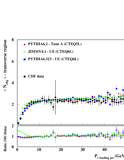
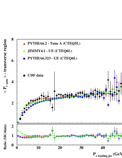
Another measurement of the underlying event was made by defining two cones in space, at the same pseudorapidity as the leading ET jet (calorimeter jet) and in the azimuthal direction, [117]. The total charged track momentum inside each of the two cones is then measured and the higher of the two values defines the “MAX” cone, with the remaining cone being labeled “MIN” cone. Figure 4.3.57 shows PYTHIA 6.323 - UE predictions for the UE compared to CDF data [117] for the of charged particles in the MAX and MIN cones for p collisions at (a) = 630 GeV and (b) 1.8 TeV. JIMMY 4.1 - UE predictions are compared to the data in fig. 4.3.58. Both tunings describe the data with good agreement, however, this only became possible by tuning the parameters of the minimum pt cut-off to include the correct energy dependence in both generators (PARP(82), (89) and (90) for PYTHIA 6.3 and PTJIM for JIMMY 4.1).
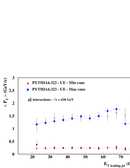
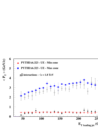
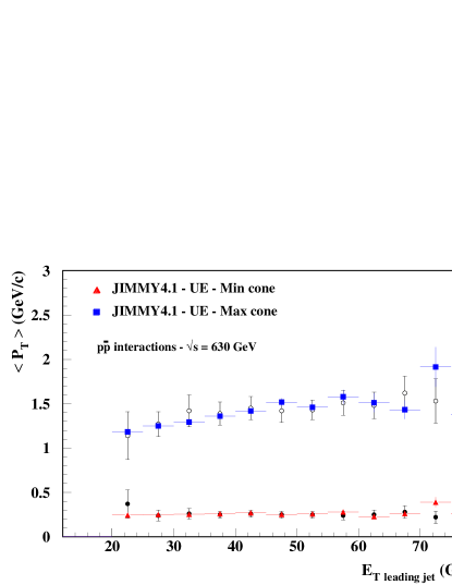
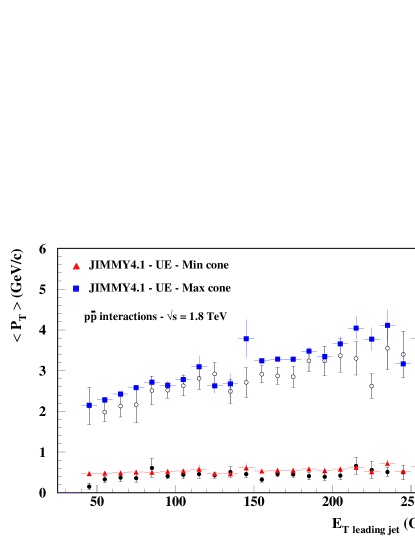
Tuning the JIMMY parameter PTJIM to include an energy dependent factor made it possible to describe the MAX-MIN distributions at different energies. Just to illustrate what would be the result of not adding the energy dependent factor in PTJIM, in fig. 4.3.59, JIMMY4.1 with PTJIM fixed by comparisons to the = 1.8 TeV distributions to PTJIM=2.8, is compared to the = 630 GeV MAX-MIN data. The predictions underestimate the data, indicating that PTJIM has to be reduced in order to describe the data.
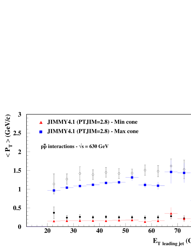
The agreement between predictions and data seen in figs. 4.3.57 and 4.3.58 for the in MAX and MIN cones is not reproduced in the comparisons of distributions for p collisions at = 1.8 TeV shown in fig. 4.3.60. There is no data available for the distributions for p collisions at = 630 GeV. Both PYTHIA 6.323 - UE and JIMMY 4.1 - UE overestimate the data. This indicates that neither model is describing the ratio / as seen in the data. This certainly needs to be improved in future tunings.
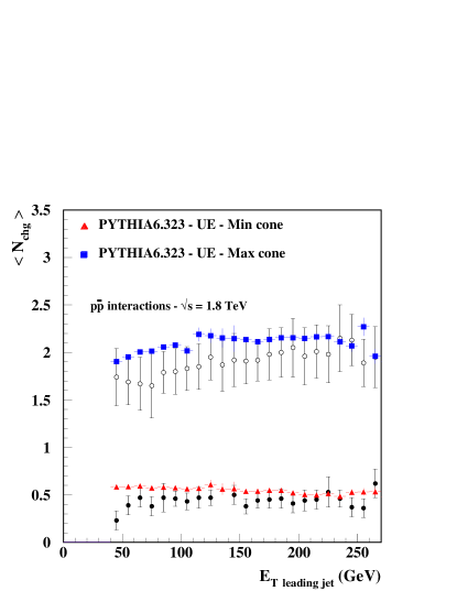
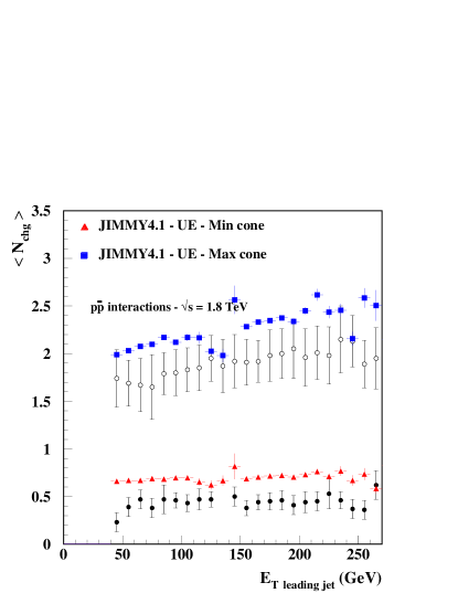
LHC predictions
Some predictions for the underlying event energy at the LHC are shown in Fig. 4.3.61. It shows PYTHIA 6.323 - UE (table 4.3.9), JIMMY 4.1 - UE (table 4.3.8) and PYTHIA 6.2 - Tune A predictions for the average multiplicity in the underlying event for LHC pp collisions. The CDF data (p collisions at = 1.8 TeV.) for the average multiplicity in the UE is also included in fig. 4.3.61.
A close inspection of predictions for the underlying event given in fig. 4.3.61 shows that the average charged particle multiplicity in the underlying event for leading jets with P GeV reaches a plateau at charged particles according to PYTHIA 6.2 - Tune A, for JIMMY 4.1 - UE and according to PYTHIA 6.323 - UE. Expressed as particle densities per unit , where the underlying event phase-space is given by [104, 107], these multiplicities correspond to 1.12, 1.43 and 1.79 charged particles per unit (pGeV), as predicted by PYTHIA 6.2 - Tune A, JIMMY 4.1 - UE, and PYTHIA 6.323 - UE, respectively. The shape of the distributions also shows significant differences between the model predictions. The shape of the multiplicity distribution generated by PYTHIA 6.323 - UE is considerably different from the other two models in the region of P GeV.
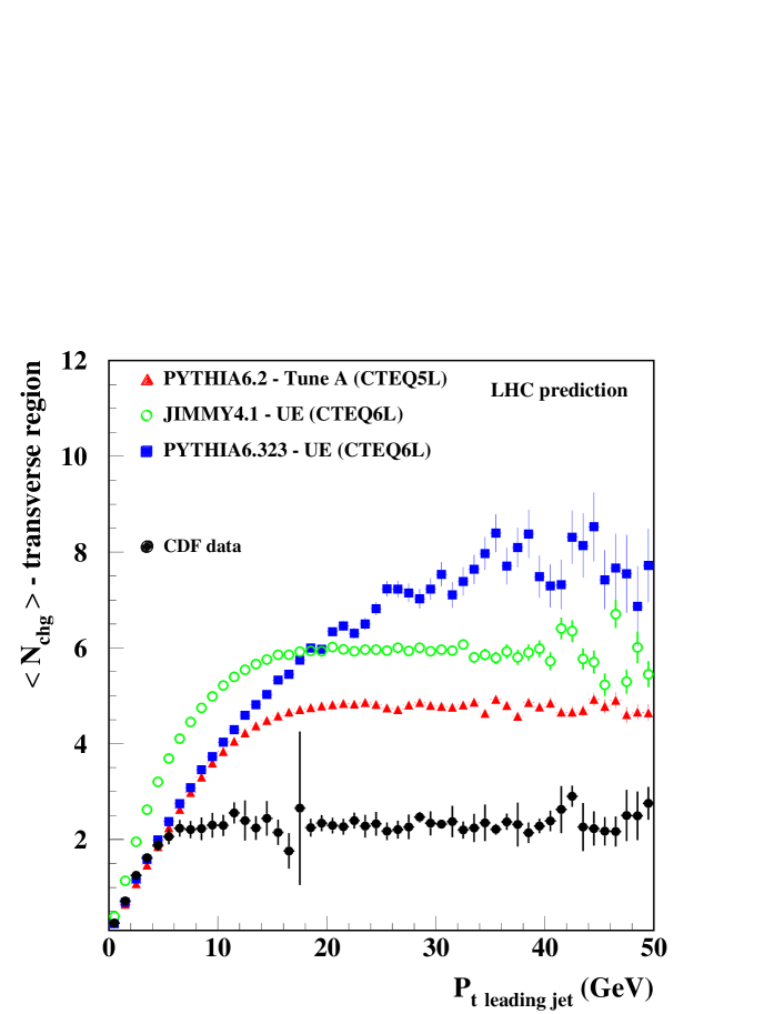
It is clear that (1) all predictions lead to a substantially larger underlying event energy at the LHC than at the Tevatron and (2) there are large differences among the predictions from the various models. Investigations are continuing trying to reduce the energy extrapolation uncertainty of these models. This measurement will be one of the first to be performed at the LHC and will be used for subsequent Monte Carlo tunings for the LHC.
5 Diffractive Physics
5.1 Large Multigap Diffraction at LHC
Contributed by: Goulianos
The large rapidity interval available at the Large Hadron Collider offers an arena in which the QCD aspects of diffraction may be explored in an environment free of gap survival complications using events with multiple rapidity gaps.
Soft Diffraction
Diffractive processes are characterized by large rapidity gaps, defined as regions of (pseudo)rapidity 888We use pseudorapidity, , and rapidity, , interchangeably. in which there is no particle production. Diffractive gaps are presumed to be produced by the exchange of a color singlet quark/gluon object with vacuum quantum numbers referred to as the Pomeron [120, 121] (the present paper contains excerpts from these two references).
Traditionally diffraction had been treated in Regge theory using an amplitude based on a simple Pomeron pole and factorization. This approach was successful at energies below GeV [122], but as collision energies increased to reach 1800 GeV at the Fermilab Tevatron the SD cross section was found to be suppressed by a factor of relative to the Regge-based prediction [123]. This blatant breakdown of factorization was traced back to the energy dependence of the Regge theory ,
| (5.1.10) |
which is faster than that of , so that at high unitarity would have to be violated if factorization held.
In contrast to the Regge theory prediction of Eq. (5.1.10), the measured SD -distribution shows no explicit -dependence (-scaling) over a region of spanning six orders of magnitude [124]. Thus, factorization appears to yield to -scaling. This is a property built into the Renormalization Model of hadronic diffraction, in which the Regge theory Pomeron flux is renormalized to unity [125].
In a QCD inspired approach, the renormalization model was extended to central and multigap diffractive processes [126], an example of which is the four-gap process shown schematically in Fig 5.1.62. In this approach cross sections depend on the number of wee partons [127] and therefore the total cross section is given by
| (5.1.11) |
where is the rapidity region in which there is particle production. Since, from the optical theorem, , the full parton model amplitude may be written as
| (5.1.12) |
where is a simple parameterization of the -dependence of the amplitude. On the basis of this amplitude, the cross section of the four-gap process of Fig. 5.1.62 takes the form
| (5.1.13) |
where the term in square brackets is the total cross section at the reduced -value, defined through , (one for each gap) is the QCD color factor for gap formation, the gap probability is the amplitude squared for elastic scattering between two diffractive clusters or between a diffractive cluster and a surviving proton with form factor , and is the (re)normalization factor defined as the gap probability integrated over all 10 independent variables , , , and .
The renormalization factor is a function of only. The color factors are and for gluon and quark color-singlet exchange, respectively. Since the reduced energy cross section is properly normalized, the gap probability is (re) normalized to unity. The quark to gluon fraction, and thereby the Pomeron intercept parameter may be obtained from the inclusive parton distribution functions (PDFs) [120]. Thus, normalized differential multigap cross sections at may be fully derived from inclusive PDFs and QCD color factors without any free parameters.
The exponential dependence of the cross section on leads to a renormalization factor independent of the number of gaps in the process. This remarkable property of the renormalization model, which was confirmed in two-gap to one-gap cross section ratios measured by the CDF Collaboration (see [120]), suggests that multigap diffraction can be used as a tool for exploring the QCD aspects of diffraction in an environment free of rapidity gap suppression effects. The LHC with its large rapidity coverage provides the ideal arena for such studies.
Hard Diffraction
Hard diffraction processes are those in which there is a hard partonic scattering in addition to the diffractive rapidity gap. SD/ND ratios for , dijet, -quark, and production at 1800 GeV measured by the CDF Collaboration are approximately equal (), indicating that the rapidity gap formation probability is largely flavor independent. However, the SD structure function measured from dijet production is suppressed by relative to expectations based on diffractive PDFs measured from diffractive DIS at HERA.
A modified version of our QCD approach to soft diffraction can be used to describe hard diffractive processes and has been applied to diffractive DIS at HERA, , and diffractive dijet production at the Tevatron, in [121]. The hard process generally involves several color “emissions” from the surviving proton, the sum of which comprises a color singlet exchange with vacuum quantum numbers. Two of these emissions are of special interest, one at from the proton’s hard PDF at scale , which causes the hard scattering, and another at (fractional momentum loss of the diffracted nucleon) from the soft PDF at GeV2, which neutralizes the exchanged color and forms the rapidity gap. Neglecting the -dependence, the diffractive structure function could then be expressed as the product of the inclusive hard structure function and the soft parton density at ,
| (5.1.14) |
where are QCD color factors, is the parameter of a power law fit to the hard structure function in the region , is a normalization factor, and .
At high at HERA, where factorization is expected to hold [125, 128], is the nominal normalization factor of the soft PDF. This factor is constant, leading to two important predictions, which are confirmed by the data:
i) The Pomeron intercept in diffractive DIS (DDIS) is -dependent and equals the average value of the soft and hard intercepts:
ii) The ratio of DDIS to DIS structure functions at fixed is independent of and :
| (5.1.15) |
At the Tevatron, where high soft parton densities lead to saturation, must be renormalized to
| (5.1.16) |
where and . Thus, the diffractive structure function acquires a term , and the ratio of the diffractive to inclusive structure functions a term . This prediction is confirmed by CDF data, where the -dependence of the diffractive to inclusive ratio was measured to be (see [120]).
A comparison 999Performed by the author and K. Hatakeyama (see [120]) using CDF published data and preliminary H1 diffractive parton densities [129]. between the diffractive structure function measured on the proton side in events with a leading antiproton to expectations from diffractive DIS at HERA showed approximate agreement, indicating that factorization is largely restored for events that already have a rapidity gap. Thus, as already mentioned for soft diffraction, events triggered on a leading proton at LHC provide an environment in which the QCD aspects of diffraction may be explored without complications arising from rapidity gap survival.
Proposed program of multigap diffraction at LHC
The rapidity span at LHC running at TeV is as compared to at the Tevatron. This suggests the following program for studies of non-suppressed diffraction:
-
•
Trigger on two forward rapidity gaps of (one on each side of the interaction point), or equivalently on forward protons of fractional longitudinal momentum loss , and explore the central rapidity region of , which has the same width as the entire rapidity region of the Tevatron. In such an environment, the ratio of the rate of dijet events with a gap between jets to that without a gap, +[jet-gap-jet]+ to +[jet-jet]+, should rise from its value of % at the Tevatron to %.
-
•
Trigger on one forward gap of or on a proton of , in which case the rapidity gap available for non-suppressed diffractive studies rises to 17 units.
5.2 Hard diffraction at the LHC and the Tevatron using double pomeron exchange
Contributed by: Royon
Hard diffraction at the LHC has brought much interest recently related to diffractive Higgs and SUSY production [130]. It is thus important that the different models available can be tested at the Tevatron before the start of the LHC. In this contribution, we will consider only one model based on the Bialas-Landshoff approach [131, 132], and more details about other models and their implications can be found in [130] and the references therein.
Theoretical framework
We distinguish in the following the so called inclusive and exclusive models for diffraction. We call exclusive models the models where almost the full energy available in the center of mass is used to produce the heavy object (dijets, Higgs, diphoton, etc.). In other words, we get in the final state the diffractive protons (which can be detected in roman pot detectors) and the heavy state which decays in the main detector. The inclusive diffraction corresponds to events where only part of the available energy is used to produce the heavy object diffractively. For this model, we assume the pomeron is made of quarks and gluons (we take the gluon and quark densities from the HERA measurements in shape and the normalisation from Tevatron data), and a quark or a gluon from the pomeron is used to produce the heavy state. Thus the exclusive model appears to be the limit where the gluon in the pomeron is a distribution in this framework or in other words, there is no pomeron remnants in exclusive events. We will see in the following that this distinction is quite relevant for experimental applications.
Exclusive model
Let us first introduce the model [133] we shall use for describing exclusive production. In [133], the diffractive mechanism is based on two-gluon exchange between the two incoming protons. The soft pomeron is seen as a pair of gluons non-perturbatively coupled to the proton. One of the gluons is then coupled perturbatively to the hard process while the other one plays the rôle of a soft screening of colour, allowing for diffraction to occur. We will give here the formulae for either the SUSY Higgs boson, or the pairs production and other formulae for standard model Higgs bosons, , diphoton or dijet production can be found in [131, 132]. The corresponding cross-sections for Higgs bosons and production read:
where, in both equations, the variables and denote respectively the transverse momenta and fractional momentum losses of the outgoing protons. In the second equation, and are respectively the squark transverse momenta and rapidities. are the hard production cross-sections which are given later on. The model normalisation constants are fixed from the fit to dijet diffractive production, while the ratio is fixed theoretically [131, 132].
In the model, the soft pomeron trajectory is taken from the standard Donnachie-Landshoff parametrisation [134], namely , with and . are kept as in the original paper [133] for the SM Higgs and pairs. Note that, in this model, the strong (non perturbative) coupling constant is fixed to a reference value which will be taken from the fit to the observed centrally produced diffractive dijets.
In order to select exclusive diffractive states, it is required to take into account the corrections from soft hadronic scattering. Indeed, the soft scattering between incident particles tends to mask the genuine hard diffractive interactions at hadronic colliders. The formulation of this correction [135] to the scattering amplitudes consists in considering a gap survival probability. The correction factor is commonly evaluated to be of order for the QCD exclusive diffractive processes at the LHC.
Inclusive model
Let us now discuss the inclusive models. We first notice that both models are related, since they are both based on the Bialas Landshoff formalism. The main difference, as we already mentionned, is that the exclusive model is a limit of the inclusive model where the full energy available is used in the interaction. The inclusive models implies the knowledge of the gluon and quark densities in the pomeron. Whereas exclusive events are still to be observed, inclusive diffraction has been studied already in detail at UA8 and then at HERA and Tevatron.
The inclusive mechanism is based on the idea that a Pomeron is a composite system, made itself from quarks and gluons. In our model, we thus apply the concept of Pomeron structure functions to compute the inclusive diffractive Higgs boson cross-section. The H1 measurement of the diffractive structure function [137] and the corresponding quark and gluon densities are used for this purpose. This implies the existence of Pomeron remnants and QCD radiation, as is the case for the proton. This assumption comes from QCD factorisation of hard processes. However, and this is also an important issue, we do not assume Regge factorisation at the proton vertices, i.e. we do not use the H1 Pomeron flux factors in the proton or antiproton.
Regge factorisation is known to be violated between HERA and the Tevatron. Moreover, we want to use the same physical idea as in the exclusive model [133], namely that a non perturbative gluon exchange describes the soft interaction between the incident particles. In practice, the Regge factorisation breaking appears in three ways in our model:
i) We keep as in the original model of Ref [133] the soft Pomeron trajectory with an intercept value of 1.08.
ii) We normalize our predictions to the CDF Run I measurements, allowing for factorisation breaking of the Pomeron flux factors in the normalisation between the HERA and hadron colliders 101010Indeed, recent results from a QCD fit to the diffractive structure function in H1 [138] show that the discrepancy between the gluonic content of the Pomeron at HERA and Tevatron appears mainly in normalisation..
iii) The color factor derives from the non-factorizable character of the model, since it stems from the gluon exchange between the incident hadrons. We will see later the difference between this and the factorizable case.
The formulae for the inclusive production processes considered here follow. We have, for dijet production111111We call “dijets” the produced quark and gluon pairs., considering only the dominant gluon-initiated hard processes:
and for Higgs boson production:
In the above, the (resp. ) are the Pomeron gluon (resp. quark) densities, and (resp. ) are the Pomeron’s momentum fractions carried by the gluons (resp. quarks) involved in the hard process. We use as parametrizations of the Pomeron structure functions the fits to the diffractive HERA data performed in [139, 138]. Additional formulae concerning for instance inclusive diffractive production of dileptons or diphotons are given in [131, 132].
Both the inclusive and exclusive productions have been implemented in a generator called DPEMC, which has been interfaced with a fast simulation of the DØ , CDF, ATLAS and CMS detectors.
Experimental context
In this section, we discuss mainly the parameters which we use to simulate the detectors at the LHC. The simulation will be valid for both CMS and ATLAS detectors. The analysis is based on a fast simulation of the CMS detector at the LHC. The calorimetric coverage of the CMS experiment ranges up to a pseudorapidity of . The region devoted to precision measurements lies within , with a typical resolution on jet energy measurement of , where is in GeV, and a granularity in pseudorapidity and azimuth of .
In addition to the central CMS detector, the existence of roman pot detectors allowing to tag diffractively produced protons, located on both sides, is assumed [140]. The acceptance and resolution have been derived for each device using a complete simulation of the LHC beam parameters. The combined acceptance is for ranging from to , where is the proton fractional momentum loss. The acceptance limit of the device closest to the interaction point is 0.02.
In exclusive double Pomeron exchange, the mass of the central heavy object is given by , where and are the proton fractional momentum losses measured in the roman pot detectors. At this level, we already see the advantages of the exclusive events. Since, there is no energy loss due to additional radiation or pomeron remnants, we can reconstruct the total diffractive mass, which means the mass of the diffractively produced object (the Higgs, dijets, , , events, pairs…), very precisely using the kinematical measurements from the roman pot detectors. The mass resolution is thus coming directly from the resolution which is expected to be of the order of 1%. For inclusive events, the mass resolution will not be so good since part of the energy is lost in radiation, which means that we measure the mass of the heavy object produced diffractively and the pomeron remnants together very precisely. To get a good mass resolution using inclusive events requires a good measurement of the pomeron remnants and soft radiation and being able to veto on it.
Existence of exclusive events
While inclusive diffraction has already been observed at many colliders, the question arises whether exclusive events exist or not since they have never been observed so far. This is definitely an area where the Tevatron experiments can help to test the models and show evidence for the existence of exclusive events if any. It is crucial to be able to test the different models before the start of the LHC. The DØ and CDF experiments at the Tevatron (and the LHC experiments) are ideal places to look for exclusive events in dijet or channels for instance where exclusive events are expected to occur at high dijet mass fraction. So far, no evidence of the existence of exclusive events has been found. The best way to show evidence of the existence of exclusive events would be the measurement of the ratio of the diphoton to the dilepton cross sections as a function of the diphoton/dilepton mass ratio (the diphoton-dilepton mass ratio being defined as the diphoton-dilepton mass divided by the total diffractive mass). The reason is quite simple: it is possible to produce exclusively diphoton but not dilepton directly since () is possible but not () directly at leading order. The ratio of the diphoton to the dilepton cross section should show a bump or a change of slope towards high diphoton-dilepton masses if exclusive events exist. Unfortunately, the production cross section of such events is small and it will probably not be possible to perform this study before the start of the LHC.
Another easier way to show the existence of such events would be to study the correlation between the gap size measured in both and directions and the value of measured using roman pot detectors, which can be performed in the DØ experiment. The gap size between the pomeron remnant and the protons detected in roman pot detector is of the order of for usual diffractive events (the measurement giving a slightly smaller value to be in the acceptance of the forward detectors) while exclusive events show a much higher value for the rapidity gap since the gap occurs between the jets (or the ) and the proton detected in roman pot detectors (in other words, there is no pomeron remnant) 121212To distinguish between pure exclusive and quasi-exclusive events (defined as inclusive diffractive events where little energy is taken away by the pomeron remnants, or in other words, events where the mass of the heavy object produced diffractively is almost equal to the total diffractive mass), other observables such as the ratio of the cross sections of double diffractive production of diphoton and dilepton, or the -jets to all jets are needed [131, 132]. Another observable leading to the same conclusion would be the correlation between computed using roman pot detectors and using only the central detector.
Another way to access the existence of exclusive events would be via QCD evolution. If one assumes that the DGLAP evolution equations work for parton densities in the pomeron, it is natural to compare the predictions of perturbative QCD with for instance dijet production in double pomeron exchange as a function of the dijet mass fraction (defined as the ratio of the dijet mass divided by the total diffractive mass) for different domains in diffractive mass. It has been shown that the dependence of the exclusive production cross section as a function of the dijet mass is much larger than the one of the inclusive processes. In other words, if exclusive events exist, it is expected that the evolution of the dijet cross section in double pomeron exchanges as a function of dijet mass fraction in bins of dijet masses will be incompatible with standard QCD DGLAP evolution, and will require an additional contribution, namely the exclusive ones 131313Let us note that one should also distinguish this effect from higher order corrections, and also from higher twist effects, which needs further studies.. It will be quite interesting to perform such an analysis at the Tevatron if statistics allows.
Results on diffractive Higgs production
Results are given in Fig. 5.2.63(a) for a Higgs mass of 120 GeV, in terms of the signal to background ratio S/B, as a function of the Higgs boson mass resolution. Let us notice that the background is mainly due the exclusive production. However the tail of the inclusive production can also be a relevant contribution and this is related to the high gluon density which is badly known as present. It is thus quite important to constrain these distributions using Tevatron data as suggested in a next section.
In order to obtain an S/B of 3 (resp. 1, 0.5), a mass resolution of about 0.3 GeV (resp. 1.2, 2.3 GeV) is needed. The forward detector design of [140] claims a resolution of about 2.-2.5 GeV, which leads to a S/B of about 0.4-0.6. Improvements in this design would increase the S/B ratio as indicated on the figure. As usual, this number is enhanced by a large factor if one considers supersymmetric Higgs boson production with favorable Higgs or squark field mixing parameters.
The cross sections obtained after applying the survival probability of 3% at the LHC as well as the S/B ratios are given in Table 5.2.10 if one assumes a resolution on the missing mass of about 1 GeV (which is the most optimistic scenario). The acceptances of the roman pot detectors as well as the simulation of the CMS detectors have been taken into account in these results.
Let us also notice that the missing mass method will allow to perform a mass measurement using exclusive (or quasi-exclusive) events in double Pomeron exchanges, and QED processes [141]. The advantage of the QED processes is that their cross section is perfectly known and that this measurement only depends on the mass resolution and the roman pot acceptance. In the same way, it is possible to measure the mass of the top quark in events in double Pomeron exchanges [141] as we will see in the following.
| cross | signal | backg. | S/B | ||
|---|---|---|---|---|---|
| section | |||||
| 120 | 3.9 | 27.1 | 28.5 | 0.95 | 5.1 |
| 130 | 3.1 | 20.6 | 18.8 | 1.10 | 4.8 |
| 140 | 2.0 | 12.6 | 11.7 | 1.08 | 3.7 |
The diffractive SUSY Higgs boson production cross section is noticeably enhanced at high values of and since we look for Higgs decaying into , it is possible to benefit directly from the enhancement of the cross section contrary to the non diffractive case. A signal-over-background up to a factor 50 can be reached for 100 fb-1 for [142]. We give in Fig. 5.2.63(b) the signal-over-background ratio for different values of for a Higgs boson mass of 120 GeV.

Threshold scan method: , top and stop mass measurements
We propose a new method to measure heavy particle properties via double photon and double pomeron exchange (DPE), at the LHC [141]. In this category of events, the heavy objects are produced in pairs, whereas the beam particles often leave the interaction region intact, and can be measured using very forward detectors.
Pair production of bosons and top quarks in QED and double pomeron exchange are described in detail in this section. pairs are produced in photon-mediated processes, which are exactly calculable in QED. There is basically no uncertainty concerning the possibility of measuring these processes at the LHC. On the contrary, events, produced in exclusive double pomeron exchange, suffer from theoretical uncertainties since exclusive diffractive production is still to be observed at the Tevatron, and other models lead to different cross sections, and thus to a different potential for the top quark mass measurement. However, since the exclusive kinematics are simple, the model dependence will be essentially reflected by a factor in the effective luminosity for such events.
Explanation of the methods
We study two different methods to reconstruct the mass of heavy objects double diffractively produced at the LHC. The method is based on a fit to the turn-on point of the missing mass distribution at threshold.
One proposed method (the “histogram” method) corresponds to the comparison of the mass distribution in data with some reference distributions following a Monte Carlo simulation of the detector with different input masses corresponding to the data luminosity. As an example, we can produce a data sample for 100 fb-1 with a top mass of 174 GeV, and a few MC samples corresponding to top masses between 150 and 200 GeV by steps of. For each Monte Carlo sample, a value corresponding to the population difference in each bin between data and MC is computed. The mass point where the is minimum corresponds to the mass of the produced object in data. This method has the advantage of being easy but requires a good simulation of the detector.
The other proposed method (the “turn-on fit” method) is less sensitive to the MC simulation of the detectors. As mentioned earlier, the threshold scan is directly sensitive to the mass of the diffractively produced object (in the W case for instance, it is sensitive to twice the mass). The idea is thus to fit the turn-on point of the missing mass distribution which leads directly to the mass of the produced object, the boson. Due to its robustness, this method is considered as the “default” one in the following.
Results
To illustrate the principle of these methods and their achievements, we apply them to the boson and the top quark mass measurements in the following, and obtain the reaches at the LHC. They can be applied to other threshold scans as well. The precision of the mass measurement (0.3 GeV for 300 fb-1) is not competitive with other methods, but provides a very precise calibration of the roman pot detectors. The precision of the top mass measurement is however competitive, with an expected precision better than 1 GeV at high luminosity. The resolution on the top mass is given in Fig. 5.2.66(a) as a function of luminosity for different resolutions of the roman pot detectors.
The other application is to use the so-called “threshold-scan method” to measure the stop mass in exclusive events. The idea is straightforward: one measures the turn-on point in the missing mass distribution at about twice the stop mass. After taking into account the stop width, we obtain a resolution on the stop mass of 0.4, 0.7 and 4.3 GeV for a stop mass of 174.3, 210 and 393 GeV for a luminosity (divided by the signal efficiency) of 100 fb-1. We notice that one can expect to reach typical mass resolutions which can be obtained at a linear collider. The process is thus similar to those at linear colliders (all final states are detected) without the initial state radiation problem.
The caveat is of course that production via diffractive exclusive processes is model dependent, and definitely needs the Tevatron data to test the models. It will allow to determine more precisely the production cross section by testing and measuring at the Tevatron the jet and photon production for high masses and high dijet or diphoton mass fraction.
How to constrain the high gluon using Tevatron and LHC data?
In this section, we would like to discuss how we can measure the gluon density in the pomeron, especially at high since the gluon in this kinematical domain shows large uncertainties and this is where the exclusive contributions should show up if they exist. To take into account, the high- uncertainties of the gluon distribution, we chose to multiply the gluon density in the pomeron measured at HERA by a factor where varies between -1.0 and 1.0. If is negative, we enhance the gluon density at high by definition, especially at low .
The measurement of the dijet mass fraction at the Tevatron for two jets with a greater than 25 GeV for instance in double pomeron exchange is indeed sensitive to these variations in the gluon distribution. The dijet mass fraction is given in Fig 3 and 4 which shows how the Tevatron data can effectively constrain the gluon density in the pomeron [138]. Another possibility to measure precisely the gluon distribution in the pomeron at high would be at the LHC the measurement of the cross section in double pomeron exchange in inclusive events [143]. By requiring the production of high mass objects, it is possible to assess directly the tails of the gluon distribution. In Fig. 5.2.65, we give the total mass reconstructed in roman pot detectors for double tagged events in double pomeron exchanges and the sensitivity to the gluon in the pomeron.


New possible measurement of survival probabilities in the DØ experiment
We propose a new measurement to be performed at the Tevatron, in the DØ experiment [135], which can be decisive to distinguish between Pomeron-based and soft colour interaction models of hard diffractive scattering. This measurement allows to test directly the survival probability parameters as well which is fundamental to predict correctly the exclusive diffractive Higgs production at the LHC. The discriminative potential of our proposal takes its origin in the factorization breaking properties which were already observed at the Tevatron. The explanation given to this factorization breaking in Pomeron-based models is the occurrence of large corrections from the survival probabilities, which is the probability to keep a diffractive event signed either by tagging the proton in the final state or by requiring the existence of a rapidity gap in the event. By contrast with Pomeron models, the soft color interaction models are by nature, non factorizable. The initial hard interaction is the generic standard dijet production, accompanied by the full radiative partons. Then, a phenomenological soft color interaction is assumed to modify the overall color content, allowing for a probability of color singlet exchange and thus diffraction.
The forward detector apparatus in the DØ experiment at the Tevatron, Fermilab, has the potential to discriminate between the predictions of the two approaches in hard “double” diffractive production, e.g. of centrally produced dijets, by looking to the azimuthal distributions of the outgoing proton and antiproton with respect to the beam direction. This measurement relies on tagging both outgoing particles in roman pot detectors installed by the D0 experiment.
The FPD consists of eight quadrupole spectrometers, four being located on the outgoing proton side, the other four on the antiproton side. On each side, the quadrupole spectrometers are placed both in the inner (Q-IN), and outer (Q-OUT) sides of the accelerator ring, as well as in the upper (Q-UP) and lower (Q-DOWN) directions. They provide almost full coverage in azimuthal angle . The dipole spectrometer, marked as D-IN, is placed in the inner side of the ring, in the direction of outgoing antiprotons.
Each spectrometer allows to reconstruct the trajectories of outgoing protons and antiprotons near the beam pipe and thus to measure their energies and scattering angles. Spectrometers provide high precision measurement in and variables, where and are the total and transverse momenta of the outgoing proton or antiproton, and is the beam energy. The dipole detectors show a good acceptance down to for and the quadrupole detectors are sensitive on outgoing particles down to GeV2 for , which allows to get a good acceptance for high mass objects produced diffractively in the DØ main detector. For our analysis, we use a full simulation of the FPD acceptance in and [144].
We suggest to count the number of events with tagged and for different combinations of FPD spectrometers. For this purpose, we define the following configurations for dipole-quadrupole tags (see Fig. 2): same side (corresponding to D-IN on side and Q-IN on side and thus to degrees), opposite side (corresponding to D-IN on side and Q-OUT on side, and thus to degrees), and middle side (corresponding to D-IN on side and Q-UP or Q-DOWN on side and thus to degrees). We define the same kinds of configurations for quadrupole-quadrupole tags (for instance, the same side configuration corresponds to sum of the four possibilities: both protons and antiprotons tagged in Q-UP, Q-DOWN, Q-IN or Q-OUT).
In Table 2, we give the ratios and (note that we divide by 2 to get the same domain size in ) for the different models. In order to obtain these predictions, we used the full acceptance in and of the FPD detector [144]. Moreover we computed the ratios for two different tagging configurations namely for tagged in dipole detectors, and in quadrupoles, or for both and tagged in quadrupole detectors.
In Table 2, we notice that the dependence of the event rate ratio for the SCI [145, 146] model is weak, whereas for the POMWIG [145, 146] models the result show important differences specially when both and are tagged in quadrupole detectors. This measurement can be performed even at low luminosity (1 week of data) if two jets with a transverse momentum greater than 5 GeV are required.
With more luminosity, we also propose to measure directly the dependence between the outgoing protons and antiprotons using the good coverage of the quadrupole detectors in which will allow to perform a more precise test of the models.
| Config. | model | midd./ | opp./ |
|---|---|---|---|
| same | same | ||
| Quad. | SCI | 1.3 | 1.1 |
| Dipole | Pom. 1 | 0.36 | 0.18 |
| Pom. 2 | 0.47 | 0.20 | |
| Quad. | SCI | 1.4 | 1.2 |
| Quad. | Pom. 1 | 0.14 | 0.31 |
| Pom. 2 | 0.20 | 0.049 |
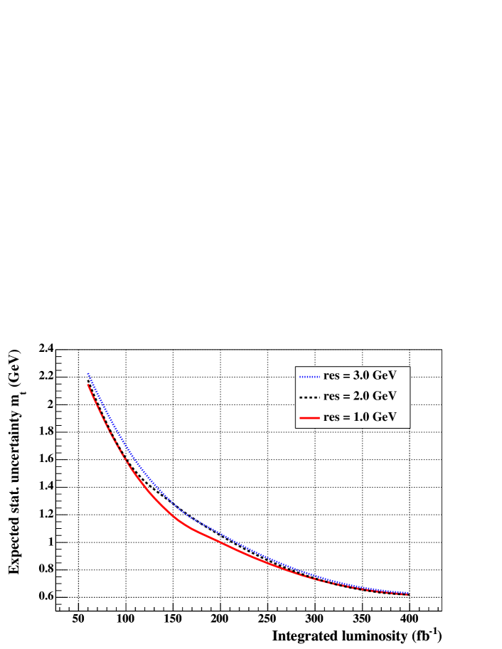
Acknowledgments
These results come from a fruitful collaboration with M. Boonekamp, J. Cammin, A. Kupco, S. Lavignac, R. Peschanski and L. Schoeffel.
5.3 Diffraction and Central Exclusive Production
Contributed by: Albrow, De Roeck
Diffractive physics covers the class of interactions that contain large rapidity gaps (typically 4 units) with no hadrons. This implies color singlet exchange, requiring two or more gluons with a (minor) contribution of . This is a frontier of QCD, not fully understood but where much progress has been made through experiments at the Tevatron and HERA. Here we consider two areas in hadron-hadron collisions, diffraction and a special subset central exclusive production. The latter has become very topical as a window on the Higgs sector and BSM physics at the LHC. To this end the FP420 R&D collaboration [147] aims to add high precision forward proton detectors to CMS and/or ATLAS.
Central exclusive processes are defined as where is a fully measured simple state such as and represents a large ( 4) rapidity gap. As there are no additional particle produced, precise measurements of both forward protons give the mass of the central exclusive state. There are several other important advantages in these processes, as described below, and the Higgs and di-boson sectors are most interesting. Measurements of all the other listed processes tend to be directed towards understanding these electroweak processes better, although they are at the same time probes of QCD in an important region (the perturbative-non-perturbative boundary). The and states are purely QED with negligible QCD corrections.
If the reaction is seen at the LHC, precise proton measurements () allow one to measure the Higgs mass with 2 GeV per event, independent of the decay mode (e.g. ), as discussed in the next section. The signal: background can be 1:1, even considerably larger for MSSM Higgs. The Higgs quantum numbers (Is it a scalar? Is CP = ++?) can be determined from the azimuthal correlations. The key question is : “What is the cross section for ”? We proposed [148] that has an identical QCD structure, might be measurable at the Tevatron and, if seen, would confirm that must occur and “calibrate” the theory. The Durham group (see e.g. Ref [149, 150, 151]) calculated the cross sections and they have been incorporated into the ExHume [152] generator. CDF has now observed the process[153], confirming that the exclusive cross section for (SM) 130 GeV is 3 fb or perhaps a factor 2-3 higher, which is very encouraging.
In the MSSM the Higgs cross section can be an order of magnitude higher than in the SM, depending on tan(). In addition to observations, exclusive central produced by 2-photon exchange should be seen, fb, and final state interactions between the ’s can be studied. Exclusive and have recently been observed in CDF[153], the first time processes have been seen in hadron-hadron collisions. The reaction is important at the LHC for two reasons: (1) The cross section is very well known (QED) and it can be used to calibrate luminosity monitors, perhaps to %. The dominant uncertainty would be knowledge of the trigger, acceptance and efficiencies. (2) The forward proton momenta are very well known and can calibrate those spectrometers; the central mass scale is calibrated with the precision . Once the forward proton spectrometers are well calibrated it should be possible to use reactions such as , when there is only one interaction per crossing, to calibrate the full CMS/ATLAS calorimeter (i.e. find a global energy scale factor). Hence it is important to study these processes at the Tevatron. For example, how cleanly can one select the exclusive with pile up, by requiring no other tracks on the vertex, , and ? Unfortunately the reaction can only be seen in the absence of pile-up, requiring luminosity less than about 5.1031 cm-2 s-1, which is becoming rare, so little more can be done.
Other exclusive processes which can be studied at the Tevatron and are related to exclusive production are and
Exclusive Higgs Production
A recent development in the study of rapidity gap phenomena is the search for and measurements of the Higgs particle in central exclusive production events, shown in Fig. 5.3.67 (left). The process was first proposed for the Tevatron collider [154], pointing out that when using the missing mass calculated with respect to the two outgoing protons, a Higgs mass resolution of the order of 250 MeV could be achieved. As it turned out the cross section at the CM energy of the Tevatron is too low to be measured. The mass resolution scales approximately with , and can be 2 GeV at the LHC.
A calculation of the cross section for DPE exclusive Higgs production with at the LHC gives about 3 fb for a SM Higgs with mass of 120 GeV [155]. After exeprimental cuts (not optimized) about 10 signal events will be reconstructed for 30 fb-1, with a similar amount of background events expected in a 2 GeV mass bin. The cross sections can be up to a factor 10-20 larger for MSSM, see Fig. 5.3.67 (right). Backgrounds in the channel are suppressed at LO due to the spin selection rule. Reconstructing the Higgs mass from the missing mass to the protons
with the four momenta of the incoming beam particles and the ones of the outgoing protons, will allow to measure the Higgs mass via the missing mass technique with a resolution of 2 GeV, independent of the decay mode. For the and channels this is greatly superior to any other technique.

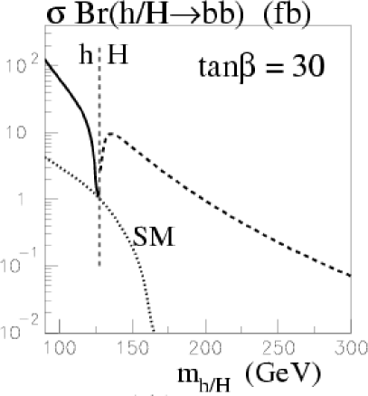
Recently also the decay has been studied. With experimental acceptances and cuts about 7 signal events are expected with 3 background events for 30 fb-1 and a S.M. Higgs mass of 160 GeV with detector cuts[156]. More channels are being studied and the phenomenology is moving forward fast.
The predictability of the cross section has been a long debate and (after some selection, when e.g. including the present limits on the exclusive di-jet production at the Tevatron) factors differences of an order of magnitude have been reported. During the HERA/LHC workshop the so called “Durham” calculations have been scrutinized and have been confirmed by other groups. Hence within the pQCD picture used it seems calculations can be used, and sophisticated predictions [155] claim an uncertainty of only a factor 2 - 3, mainly due to PDFs, but there is still some controversy. Crucial information will have to come from similar measurements to test these calculations with data. In particular exclusive di-jets, exclusive 2 photon and production are candidate processes to test the theory and already now at the Tevatron such measurements are being performed, as will be discussed further in this report.
Besides a possible discovery channel for the MSSM Higgs, and a channel to measure the decay mode, the central exclusive Higgs production also allow for CP studies via the azimuthal correlations [157]. The exclusive system is so constrained that it produces predominantly spin 0 or 2 states, and these impose different azimuthal correlations on the protons. Thus it can confirm the scalar nature of a new particle discovered and called Higgs at the LHC, a measurement otherwise difficult to make at the LHC, especially for a light Higgs. Hence this measurement will have a strong added value to the LHC physics program.
Recently it was also shown in [158] that the forward tagging of protons would be important for CP violating MSSM Higgs scenarios, where the three neutral Higgses are nearly degenerate in mass and can mix. This will lead to structures as shown in Fig. 5.3.68, and will need an experimental tool that can scan the Higgs mass region with a mass precision of about 1 GeV. The tagged protons can be such a tool, perhaps uniquely.
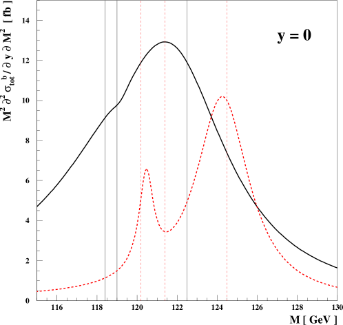
Forward Detectors at the Tevatron
At the Tevatron both experiments, CDF and D0, are equipped with very forward detectors to measure diffractively scattered protons and large rapidity particles, specifically as rapidity gap detectors. Very early (1989) CDF installed forward proton trackers in roman pots (moveable vacuum chambers that allow detectors to move very close to the beam during a store) and measured the total cross section , elastic scattering and single diffractive excitation . Elastic scattering and the total cross section are basic properties of interactions, which will be measured at the LHC by the TOTEM experiment. Unfortunately they are not very well known at the Tevatron, with three inconsistent () measurements of , and only one measurement of into the Coulomb region and none into the large region beyond 2 GeV2 (interesting from a perturbative point of view). There are no measurements yet at = 1960 GeV, although the LHC could run down to that to make a comparison of and . The first generation CDF roman pots were removed after these measurements, and for a period diffractive physics was done using large rapidity gaps, without seeing the scattered proton(s). One could demonstrate diffractive signatures for production of jets, heavy flavors () and even as a distinct class of events with 3-4 units of rapidity devoid of hadrons. (e.g. The distribution of charged hadron multiplicity or in a forward region shows a clear peak at zero). Both experiments also discovered the phenomenon of “gaps between jets” (JGJ) in which two high jets (10-50 GeV) at large opposite rapidity have a gap 4 units in between. The 4-momentum transfer2, , is huge (of order GeV2). This is presumably not the regime of a “pomeron”, but is best described as perturbative scattering accompanied by other gluon exchange(s) to cancel the color exchange and leave a gap. The relationship between these descriptions is a topical issue.
Shortly before the end of Run 1, in 1995, CDF installed a new set of roman pots on one arm () specifically to study high mass diffraction in more detail. These were a triplet of pots over about 2m in , 53m from the beam intersection. The detectors were arrays of square section scintillating fibers to give coordinates with about 100 resolution over 2cm 2cm, backed up by scintillation counters (one in each pot, put in coincidence for a trigger). Level 1 triggers required a 3-fold “pot scintillator” coincidence together with central jets or leptons. Also the forward proton detectors were read out for all events, a principle which should be followed in CMS and ATLAS. These detectors remained in Run 2 (2003 on), supplemented by Beam Shower Counters (BSC1,2,3) which were scintillation counters tightly around the beam pipe wherever they could be fitted, covering . BSC1 had 3 of lead in front to convert photons, the others were in the shadow of material (beam pipe, flanges) and detected mostly showers. These counters are used as “rapidity gap detectors”, sometimes in a L1 trigger. Another innovation in Run 2 was the “Miniplug” calorimeter covering consisting of a cylindrical tank of liquid scintillator with lead plates. The wavelength-shifting fiber readout was arranged to have very high granularity. This is used for rapidity gap physics and for triggering on very forward jets (especially for JGJ studies).
A lesson from the CDF Run 2 diffractive studies is that it is very important to cover as completely as possible the forward and very forward region for charged hadrons and photons, with the ability to trigger on and find forward rapidity gaps with little background (e.g. from particles that can miss these detectors). This was crucial in CDF e.g. for showing that the exclusive 2-photon events were really exclusive, and hopefully this will also be done at the LHC.
In Run 1 D0 studied diffractive physics only with (pseudo-)rapidity gaps, but for Run 2 they installed a system of roman pots (Forward Proton Detectors, FPD) on both arms for and detection. Three pots detected at 53m after three dipoles, almost identical to the CDF pots, with square scintillating fiber hodoscopes. Others, on both and arms, were placed behind low- quadrupoles (not dipoles). These have acceptance for normal low- running, down to 0.7 GeV2 (which misses much of the cross section for rare processes) and the momentum (and ) resolution is considerably worse than the dipole spectrometers. However because both and can be detected, elastic scattering is measurable as well as a new measurement of the total cross section (for the first time at GeV). These measurements needed a special high- run to reach a GeV2. The two-arm FPD also allows studies of double pomeron exchange with both protons measured. This has never yet been studied at the Tevatron. Low mass ( 5 GeV) states such as and can provide very interesting glueball and hybrid searches, as the soft pomeron is glue-rich and the forward proton correlations can determine central quantum numbers (spin, CP). The highest previous energy at which this was done at = 63 GeV at the ISR, and showed interesting structures in exclusive channels (e.g. ). This is a potentially rich field, both for studying diffractive mechanisms and for spectroscopy ( is rich in glueball and hybrid states). There was almost no background from non-pomeron exchange. Although for this low mass DPE there would seem to be no real advantage in much higher collision energies, depending on what D0 is able to achieve there could be an interesting program at the LHC, with high- necessary to get low acceptance in the TOTEM (and possible ATLAS?) pots. For cleanliness this needs single interactions/crossing. In D0 the forward coverage in is limited by their liquid argon calorimeter ( 4.5), so unfortunately some 3 units of forward rapidity are not covered (except for the roman pots).
Forward Physics Measurements at the Tevatron
Considering only inelastic diffraction, there have been three phases of measurements at the Tevatron.
In 1994 CDF published a study of single diffractive excitation SDE with the scattered measured in pots with drift chambers and silicon counters. Data were taken at both = 546 GeV (to equal the CERN ) and 1800 GeV. The diffractive peak extends to = 0.05 (as at the ISR) corresponding to an excited mass 300 GeV. Note that at the LHC the corresponding mass reach is 2000 GeV, well above the threshold and perhaps into the realm of new BSM physics. The differential cross section was measured and compared to parametrizations. The integrated cross sections were (546) = 7.9 0.3 mb, (1800) = 9.5 0.4 mb, about 10% of the total cross section.
In the second phase the emphasis was on rapidity gap physics (the older pots were removed). Both CDF and D0 discovered large rapidity gaps between high jets, and both found high- dijet production in SDE. CDF presented evidence for diffractive production and later D0 published both and in SDE with higher statistics. As a rule-of-thumb, about 1% of hard processes (jets, , ) are diffractive. CDF also measured diffractive production of -quarks and . If there is a rapidity gap which extends into the instrumented acceptance, the momentum loss fraction of the leading baryons can be calculated from:
where the sum is over all particles. (This follows from [] conservation.) From the relative cross sections for diffractive jets, heavy flavors (predominantly from gluons) and (predominantly from annihilation) it was possible, in a model in which the pomeron has constituents, to conclude that about 60% of its momentum is carried by gluons. As these measurements are at moderately high , typically 1000 GeV2, they are not incompatible with a mainly gluonic pomeron at low . One could also derive a diffractive structure function , which is the standard structure function conditional on a rapidity gap (or diffractive proton). Comparisons with data (HERA) showed it to be lower by an order of magnitude at the Tevatron, interpreted as a much smaller gap survival probability in collisions which have additional parton-parton interactions. This is a breakdown of factorization. Double pomeron interactions have two large rapidity gaps (and two leading protons). CDF found that the probability of a second gap, given one, is substantially larger than the probability of one gap in inelastic collisions. This is understood: in one-gap events there is no gap-spoiling additional interaction, so a second gap is not suppressed. About of hard processes have two large rapidity gaps (Double Pomeron Exchange, DPE). Single diffractive excitation of low mass and high mass (di-jets, , , heavy flavors) has been measured, but there is a case for a more complete systematic study, e.g. conditional on such massive final states, at different values. From the -dependence at fixed () one could derive a “hard pomeron” trajectory to extrapolate to the LHC. Monte Carlo event generators which have interactions and include diffraction, such as HERWIG [80] and PYTHIA [103] could then be tested and tuned, to improve predictions for the LHC. A new series of studies with measurement of forward in roman pots is described in another note[159].
The third phase of inelastic diffraction, in Run 2, has again been rapidity gap physics but with an emphasis on exclusive processes in which the central state is simple and completely measured. This is described in the next section.
Central Exclusive Measurements at the Tevatron
Central exclusive production studies at the Tevatron could have a powerful impact on the LHC program. Most interesting and very important LHC processes are exclusive Higgs boson and vector boson pair () production, , with other exotic BSM possibilities. No hadrons are produced. Measurements of the forward protons allow very good mass measurements ( 2 GeV per event) for the central state, a good signal: background ( 1:1) for a SM Higgs (higher in MSSM scenarios), and determination of the central quantum numbers. -pairs and -pairs can of course come from Higgs decay, -pairs (but not -pairs) can come from two-photon collisions, and both and could be produced with an unexpectedly high rate in some BSM models (e.g. the white pomeron [160, 161]). The two-photon cross section by two-photon exchange is about 100 fb, and final state interactions can be studied beyond the LEP-2 range. In the absence of a Higgs this could be particularly interesting. The 4-momentum constraints in exclusive processes allow reconstruction of all final states except perhaps 4-jets where the background may be too high.
It was mentioned before that there is still some level of uncertainty and perhaps even controversy on the predictions of the cross sections for central exclusive Higgs production. It is therefore very important to be able to use the Tevatron experiments to reduce the uncertainty, i.e. to calibrate the predictions. The exclusive Higgs diagram has through a top loop, with an additional gluon exchange to cancel the color and allow the protons to remain unexcited. Very similar diagrams with a -loop can produce an exclusive , probably best detectable through radiative decay:
These have a large enough cross section to be detectable at the Tevatron. CDF has preliminary evidence for exclusive production (and probably also exclusive photoproduction), with much more data currently being analyzed. The is more difficult, partly because an efficient trigger was not installed early and the cross section is much smaller, and now the luminosity is typically too high to give clean single single interactions. These processes are probably not detectable in the presence of pile-up, at least not without measuring the forward protons. (The existing pots do not have good acceptance for these low mass states.) Of course the are hadrons, unlike the H, so one may worry that these reactions do not have identical QCD amplitudes.
Exclusive di-jets provide another way of testing the theoretical calculations. CDF has triggered on events with a diffractive and two central jets and then selected events with a rapidity gap on the opposite () side (DPE candidates). They then study the distribution of , where is the total central mass, which would be near 1.0 if all the central hadrons were in just two jets. There is no peak near 1.0, but the monotonically falling distribution may have a shoulder, being a smeared-out indication of exclusivity. If one (somewhat arbitrarily) takes the cross section for events with it compares reasonably with the theoretical expectations. However the idea of “exclusive dijets” is not well defined. A high jet is dependent on a choice of algorithm, e.g. with a cone (or ) jet algorithm hadrons at an angle (or ) exceeding a cut are considered outside the jets and spoil the exclusivity. By these criteria most LEP events would not be classed as exclusive. Exclusive di-jets should be particularly suppressed (by a spin selection rule) when . (So this process could provide a clean sample of gluon jets.) CDF attempts to exploit this by studying the distribution for -tagged jets. A preliminary analysis shows a drop in the fraction of -jets as 1, intriguing but needing more data. A suppression of dijets as 1 is just what is needed to reduce di-jet background in exclusive production (for GeV).
A phenomenological analysis of the di-jet data of the Tevatron was performed in [162]. It was found that the CDF run-I data are consistent with the presence of an exclusive di-jet component, and this component should become visible in the data with the Run II statistics. An important finding is that a non-perturbative model for the central exclusive process, as included in DPEMC [163], predicts a different dijet dependence compared to ExHume, possibly allowing to discriminate between these two models. Fig. 5.3.69 shows the prediction of the distribution, where is the mass of the dijet system and the total mass of the centrally produced system, for a combination of inclusive diffractive (POMWIG) and exclusive (ExHume) central di-jet production. The figure shows also the distribution of the second highest jet in the region for Exhume and DPEMC. Finally it is worth noting that for such a measurement the jet finding algorithm needs to be optimized, a study which has not happened yet. V.Khoze and M.Ryskin propose[164] a different variable, using only the leading jet ( is the pseudorapidity of this jet in the rest frame).
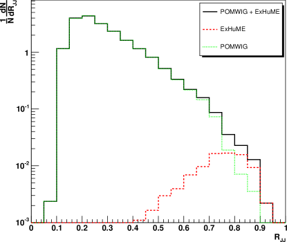
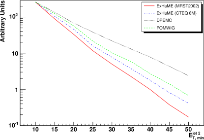
Most interesting and relevant to exclusive Higgs production at the LHC is the observation of exclusive two-photon events in CDF. We find events with GeV/c and .The (QCD) diagram is through quark loops (mainly ) with another -exchange, just as in the Higgs case. In fact from a QCD viewpoint the diagrams are identical with non-strongly interacting final states. Thus the observation (so far only 3 events …. out of about collisions!) demonstrates that the exclusive Higgs process exists (if indeed a Higgs boson exists), and also, because the cross is in agreement with the Durham group calculation, detectable, i.e in the range 1 - 10 fb. It is very important to try, if at all possible, to measure this exclusive production at the LHC, to give a closer calibration of . To do this (it can only be done without any pile-up) we need enough “single-interaction-luminosity” () to get a useful sample of events (say 100 events to give a 10% statistical uncertainty). It will (presumably) not be possible to measure the forward protons (small- and small with low-), so one must use the CDF technique of requiring the whole detector to be consistent with noise (apart from the two photon showers). To get enough rate one must go down to 5 GeV/c, and be able to trigger on that at L1. This will need some forward gap requirement at L1, from scintillators/calorimeters. A concern is whether an interaction in the previous bunch crossing (with 25 ns crossing interval) leaves enough signal in the detectors to spoil the cleanliness. This needs further study (and possibly some new counters). It is important because if the exclusive can be measured (say to 10%) the theoretical prediction for exclusive Higgs production can be made correspondingly precise, which may enable one to exclude a SM Higgs if no exclusive signal is seen, test the SM prediction if one is seen, and in the case of SUSY (or other BSM) make important measurements of the coupling.
Two photon (initial state) processes producing exclusive lepton pairs are also important for the LHC. These are highly peripheral collisions (so the protons emerge with very small ) in which photons from the protons’ field collide: . The process is pure QED (a QCD correction from simultaneous pomeron exchange is very small) and calculable to better than 0.1%. Therefore if it can be measured the luminosity for the period can be measured as well as one knows the di-lepton acceptance and efficiency. This has to be done in the presence of pile-up; if one had to require no other interaction in the crossing (as for final states) one would have to know precisely the inelastic cross section, which defeats the object. We believe that this can indeed be done, even without detecting the forward protons, thanks to three criteria : (a) the associated charged multiplicity on the vertex is = 0 (b) (c) . These events are now (belatedly) being looked for in CDF. Exclusive pairs have now been measured with no pile-up. There are two electrons with 5 GeV/c and nothing else in the detector (which extends to … the scattered protons are not seen). This is the first time 2-photon collisions have been seen in a hadron collider. The highest mass pair has GeV! Some lepton pairs, especially more forward and higher mass, are accompanied by a (anti-)proton in the roman pots. The momentum is very well known from the dimuon kinematics, the main uncertainty coming from the incident beam momentum spread . This provides an excellent (probably the best) calibration for the momentum (or missing mass) scale for the search at the LHC. This can be tested in CDF and D0, but this analysis is just starting. Hopefully there is enough data on tape now, as the CDF roman pots were removed in March 2006 as the space is needed for a new collimator (and the diffractive program winds down as the luminosity climbs; typical runs now start with with 6 interactions per crossing, and end a factor lower.) In CDF we will retain the exclusive trigger but will be low, and continue to study . However there is much data to analyze, to measure exclusive , possibly , (photoproduction), di-jets and dijets, and of course . D0 will also have low mass exclusive states in DPE with both protons tagged.
Forward Detectors at the LHC
The LHC will collide protons at a centre of mass energy of 14 TeV, starting in 2007. Hadronic collisions thus enter a new regime, and will be mainly used to unveil the mystery of electro-weak symmetry breaking and search for new physics, such as supersymmetry and extra dimensions. Recently however diffractive physics was added to the physics program of the experiments. This followed two events: the new experimental opportunities and the possibility to discover new physics via exclusive production using tagging forward protons.
The opportunities are the following. The TOTEM experiment was approved in 2004. This experiment uses forward detectors for total cross section, elastic scattering and soft diffraction measurements [165]. TOTEM uses the same interaction point as the general purpose central detector CMS. CMS also proposes to extend its forward detector capabilities, and has sent an EOI[166] to the LHCC to express its interest in forward and diffractive physics. The study of common data taking by the CMS and TOTEM detectors (roman pots and inelastic telescopes) is being addressed in a CMS/TOTEM common study group.
ATLAS has also submitted a letter of intent to build roman pot stations, primordialy for measuring the total and elastic cross section[167]. A diffractive program will be addressed in a later stage.
CMS proposes to study diffractive and low- QCD phenomena, and to enhance its detector preformance for this physics by extending its acceptance in the forward region and including the TOTEM detectors as a subdetector of CMS in common mode of data taking.
The acceptance of CMS in pseudorapidity is roughly for tracking and for calorimetry. CMS is considering extending its forward acceptance by adding a calorimeter in the region of roughly , approximately 14 m from the IP, using the available free space. Presently CASTOR is conceived to be a Tungsten/Quartz fiber calorimeter of about long, with an electromagnetic and hadronic section.
A tracker in front of CASTOR is being proposed by the TOTEM collaboration, namely the T2 inelastic event tagger. In order to be viable for CMS, the tracker must be usable at a luminosity of up to cm-2s-1 which is the nominal CMS low luminosity operation, based on a LHC optics with m. The position of the T2 tracker and CASTOR calorimeter, along the beamline and integrated with CMS, is shown in Fig. 5.3.70.
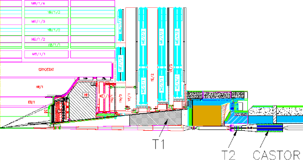
Common runs are planned for CMS and TOTEM, which will include the TOTEM roman pot (RP) detectors in the CMS readout, in order to tag protons scattered in diffractive interactions. The acceptance of the RPs is large and essentially extends over the full (fractional momentum loss of the proton) range for the high LHC optics. This will allow tagging of protons from diffractive interactions independent of and will therefore be instrumental in obtaining a deeper understanding of rapidity gap events that will be collected. Therefore there can be an interest in collecting some limited amount of data with such optics at a time and for a duration dictated by the overall LHC physics program priorities, depending on the evolution of the LHC at startup.
Roman pot detectors will be also useful for the nominal low data taking, but the acceptance is limited to with the presently planned TOTEM RPs up to 220 m. Events with smaller values can be tagged by rapidity gaps in the CMS detector, for luminosities cm-2s-1.
A zero degree calorimeter, at a distance of about 140 m from the interaction point, with both an electromagnetic and hadronic readout section is being studied for the Heavy Ion program of CMS and can also be used for the forward physics program, in particular for charge exchange processes. With these detector upgrades in the forward region CMS and TOTEM will be a unique detector having an almost complete acceptance of the events over the full rapidity range.
Note that also the ATLAS collaboration aims to add zero degree calorimeters and there is a specific experiment proposed, called LHCf, which intends to measure electromagnetic energy at zero degrees for studies relevant to cosmic rays, placed at 140 m distance of IP1. ATLAS also has a Cerenkov Counter proposal (LUCID) with acceptance over , but its use for a diffractive program has not yet been addressed.
An R&D study has been launched for beampipe detectors at distances of 420 m from the IP, ie. in the cold section of the machine. A collaboration called FP420 has been formed [147] which has submitted an LOI to the LHCC[168]. Detectors at a distance of about 420 m would be required to measure the protons from central diffractive Higgs production, e.g. the exclusive channel [169]. The technical feasibility, in particular w.r.t. the LHC machine itself, still needs to be assessed for these detectors options. The FP420 studies are largely independent from the ATLAS and CMS IP details, and will be discussed in Section 5.
Further studies include detectors between 18 m (before the TAS) and 60 m from the IP[170]. With the help of the latter the region to detect particles of could be covered. There are presently no plans yet to build such detectors.
Forward Physics Measurements at the LHC
Investigations of hadronic structure at the LHC provide new possibilities to explore important aspects of QCD. One of the main problems of QCD is the relative role of perturbative QCD and non-perturbative QCD, low- phenomena and the problem of confinement. The latter is often related to diffractive phenomena. The common study group of CMS and TOTEM is preparing for a detailed account of the physics opportunities with such a detector. The forward physics program presently contains the following topics
-
•
Soft and hard diffraction
-
–
Total cross section and elastic scattering
-
–
Gap survival dynamics, multi-gap events, soft diffraction, proton light cone studies (e.g. )
-
–
Hard diffraction: production of jets, hard photons, structure of diffractive exchange.
-
–
Double pomeron exchange events as a gluon factory
-
–
Central exclusive Higgs production (and Radion production)
-
–
SUSY & other (low mass) exotics & exclusive processes, anomalous WW production.
-
–
-
•
Low- dynamics
-
–
Parton saturation, BFKL/CCFM dynamics, proton structure, multi-parton scattering.
-
–
-
•
New forward physics phenomena
-
–
New phenomena such as Disoriented Chiral Condensates, incoherent pion emission, Centauro’s, Strangelets,…
-
–
-
•
Measurements for cosmic ray data analysis
-
•
Two-photon interactions and peripheral collisions
-
•
Forward physics in pA and AA collisions
-
•
QED processes to determine the luminosity to O(1%) e.g. .
Many of the topics on the list, except the Higgs and exotics can be studied best with luminosities of order cm-2s-1, ie. at the startup. Apart from Higgs production, discussed below, central exclusive production has been discussed as a discovery tool for other new phenomena. For example, in a color sextet quark model [160, 161], where these quarks couple strongly to the W, Z bosons and to the gluons in the pomerons, the exclusive WW production is expected to be many orders of magnitude larger that expected from SM processes and would be an easily detectable and very spectacular signal. Other possibilities include the production and detection of Radions [171]. These graviscalars appear in theories of extra dimensions, and can mix with the Higgs boson. These particles have a large coupling to gluons and are therefore expected to be produced abundantly in central exclusive production processes.
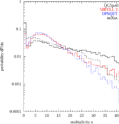
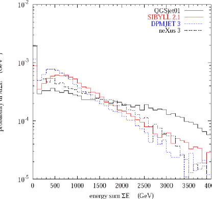
TOTEM will use a special high optics for the measurement of the total cross section. The aim is to measure the total cross section with a precision of order of 1%[174], but using a prediction of . ATLAS plans to get information on , trying to measure down to GeV2. Its often stressed that a measurement of is important for understanding the energy behaviour of the cross section at even higher energies than reachable with present machines.
The LHC data in the forward region will also help to refine the interpretation of data from ground array cosmic ray experiments. Correspondingly there is a considerable interest from the cosmic ray community in measurements from the LHC at large Feynman- or rapidity [172]. Cosmic rays interact with the gas in the atmosphere and produce extended air showers. Monte Carlo techniques are used to reconstruct the original incident particle energy and type from e.g. the measurement of the muon and electromagnetic component at the earth’s surface. The uncertainty of the models for the forward particle production – which is crucial for the energy reconstruction and incident particle type determination– is large: there exists too little collider data to constrain the models in this region. In order to make considerable improvements, measurements of the particle and energy flow at large rapidity are needed at the highest and energies, i.e. at the LHC [172]. Examples of model predictions for the total particle multiplicity and total energy flow in the forward region are shown in Fig. 5.3.71. Also the measurement of the total cross section and its diffractive components at LHC energies will be of great value and input for cosmic ray shower models. Hence the forward physics program at the LHC offers an opportunity to improve our knowledge on the leading particle production in comsic ray showers, and tune shower simulation programs.
The FP420 Proposal

FP420 is an R&D effort that has formed in 2005, in order to study the feasibility of installing proton tagging detectors in the 420 m region of the LHC. Presently 58 scientists from 29 institutes have signed the LOI. This collaboration is still open for new participants.
In order to detect the protons produced in central exclusive collisions for masses around 120 GeV, detectors in the region of about 420 m away from the interaction point are needed as shown by the acceptance calculations. Fig. 5.3.72 shows the acceptance as function of the particle (Higgs) mass for different values of detector approach to the beam. It shows that for low Higgs masses there is no acceptance with detectors at 220 m, and detectors at 420 m are needed. The differences between CMS and ATLAS for 220m are due to the different crossing angle plane at the IP.
The main task of the R&D project is to redesign the region at 420 m, which presently consists of a connecting cryostat. This 15m long cryostat needs to be redesigned such that detectors at (almost) room temperature can be installed. Present proposals for the mechanics of such detectors are mini-roman pots or a moving beampipe, as used in experiments at DESY, Hamburg. Both have advantages and disadvantages as far as precision, stability and RF issues are concerned. We aim for a precision of order of 10 micron for the position of the detectors with respect to the beam. Beam position monitors will be integrated in the moving mechanics of these detectors.
The sensitive detectors will be either 3D silicon detectors or planar silicon with 3D edges. The position resolution should be of the order of 10 microns. We also plan to use fast timing detectors with a resolution of 10-20 ps. These detectors can be used to check that the protons came form the same interaction vertex as the central tracks, and will be extremely instrumental to remove background or pile-up protons, not associated with the hard scattering in the central detector. Options for these detectors are Quartz Cerenkov detectors or gas Cerenkov detectors with microchannel PMTs.
A first report of the R&D results, including testbeam results, is planned to be completed by spring 2007, and will then be proposed as additional detectors to CMS and ATLAS. The FP420 detectors, when approved by the experiments ATLAS and CMS, can be installed during a few month shutdown. The first possible occasion in the present scheme of the LHC will be the shutdown before the year 2009 run.
Conclusion
Forward and diffractive physics is part of the Tevatron and LHC program, and a plethora of interesting measurements has and will be made. The present and forthcoming Tevatron data on central exclusive production will be vital to make firm predictions for the LHC. Several key processes are now delivering results. The LHC experiments have turned their attention to the forward region to extend detector coverage and consequently their physics program. When equipped with detectors at 420 m, the CMS and ATLAS experiment will be able to measure exclusive Higgs production, with excellent signal:background and allowing to study the spin of the centrally produced particle and its mass with a resolution of 2 GeV per event. In all aspects the experience gained with operating forward detectors at the Tevatron is extremely useful for the preparation of the these detectors for the LHC, and a continuing collaboration and information flow is essential.
6 Measurement Opportunities at the Tevatron
Introduction
In this section, we highlight some of the measurements at the Tevatron that can improve our understanding of the Standard Model and optimize our chances for finding new physics at the Tevatron and the LHC. We consider the advantages of collecting more data for some of these measurements. An accurate description of Standard Model physics is essential to predict backgrounds to new physics, and the refinements to theory that can be obtained from Tevatron measurements can be directly applied to interpreting the results from the LHC. Run II data are important inputs for improving Monte Carlo modeling of the complex event structure (this includes measurements of parton density and fragmentation functions, tuning the modeling of the underlying event, and the validation of production processes that are backgrounds to new physics searches). Such measurements help reduce errors on theory calculations as well as experimental errors, and allow a more precise comparison between theory and experiment. Since the Tevatron and the LHC will operate in very different kinematic regions, we can test for a consistent picture as predictions are extrapolated from one region to another. The Tevatron also contributes to our goal of finding convincing evidence to support a mechanism of electroweak symmetry breaking, whether it be new particles or new interactions or something unexpected. One should not rule out the possibility of new discoveries at the Tevatron, perhaps based on hints from the LHC.
To date, the Tevatron has delivered nearly 2 fb-1 of data and is projected to deliver between – fb-1 by the end of 2009 (see Figure 6.0.73 [175]). To put this number in context, the LHC is expected to have accumulated conservatively from – fb-1 of data by the end of operations in 2008. The precision of many measurements that will first be done at the Tevatron will eventually be duplicated or surpassed at the LHC with a moderate amount of data. The question can therefore be asked: “What are the advantages of running the Tevatron until the end of 2009 and accumulating 8 fb-1 before the LHC has a comparable amount of data?”
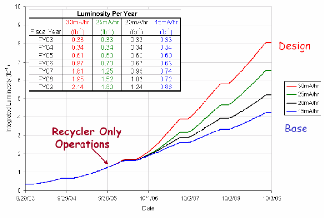
Based on experience from Run I, it takes several years to commission and fully understand a new detector and to process the data before precision measurements can be made public. At the end of collider operations, we can expect to have mature and precise measurements available which approach the measurement limits of the Tevatron. For the next several years, the Tevatron will be operating at the energy frontier, providing the opportunity to: (1) establish physics benchmarks that will be used in the initial stages of data-analysis at the LHC, until they are surpassed or complemented by in situ calibrations, (2) operate on actual (not Monte Carlo) data and refine analysis techniques necessary to finish a useful physics analysis. The continuation of this program at the Tevatron will give Fermilab–based scientists a head start in LHC analyses and provide training for the next generation of physicists and technicians. We will need to ensure that the infrastructure remains intact to allow physics analyses to continue after the halt of Tevatron operations.
The conditions, such as the kinematic region, detector resolution, and background from additional interactions, at the Tevatron and the LHC will be very different resulting in measurements with different sources of systematic errors. For some crucial measurements such as the top or mass it will be advantageous to have precise measurements from both facilities in order to be confident on the conclusions drawn from such measurements.
We are concerned that the Tevatron might be turned off prematurely, losing unique measurement opportunities that will enhance the value of future LHC or ILC measurements. A second concern is to ensure that Fermilab and the US HEP program continues to be rich and vibrant through the period of the ILC siting decision to maximize the chances the ILC will be in the US. Another concern is to have an active accelerator in the United States to provide the necessary training for the next generation of physicists who are needed to maintain a critical mass of experts in the field. We do not see a way to address these concerns without a program at Fermilab that is as broad and deep as the opportunities at the Tevatron. It should go without saying that the case has to be made based on physics in the context of the ILC being the highest priority for the future HEP program. We believe that the case to ensure that the physics potential at the Tevatron is fully exploited is very strong, and can be made convincingly.
It will be in this context that we evaluate the merits of continuing Run II beyond the year 2007. This paper does not attempt to cover all aspects of the physics program at the Tevatron but highlights some of the measurements which form a foundation for understanding the Standard Model. In addition to these measurements presented here, the Tevatron has rich programs in physics and searches for new physics which are not discussed in detail but can be found elsewhere in these proceedings as well as other publications.
The Tevatron Advantage
The Tevatron is complementary to the LHC in a number of ways, and there are specific measurements that can consequently be done either better, or with entirely different systematics, at the Tevatron. Complementary differences include:
-
•
The Tevatron is a machine, and is dominated by quark–antiquark collisions in the mass range up to 500 GeV (the ILC energy). In particular, valence quark annihilation is likely the dominant contribution to the production of new heavy states with masses comparable to the electroweak scale.
-
•
The Tevatron has a larger reach in and for measurements of energy–dependence, evolution, and scaling.
-
•
The Tevatron operates at zero crossing–angle so that missing–transverse energy in the electroweak range (100 GeV) is azimuthally symmetric and centered on the beamline.
-
•
The number of hard ( GeV) multiple–parton interactions per interaction is predicted by the present best fits to Tevatron data to be a factor of 10 lower at the Tevatron.
-
•
The shorter rapidity plateau at the Tevatron means that missing–energy due to multiple–parton interactions and initial and final state radiation is better measured.
-
•
The longer bunch length at the Tevatron allows counting of multiple vertices by separation in both space and time.
-
•
Tau identification, important in Higgs physics, using detection by sampling in orthogonal views in a “shower–max” detector is unique to the Tevatron (CDF).
-
•
Triggering on displaced vertices from heavy particles with lifetimes ( and exotics) in an all–purpose detector is unique to the Tevatron.
-
•
Fewer extra collisions per beam crossing helps in searches for rare exclusive processes that veto jets, e.g. rapidity gaps, Vector Boson Fusion (VBF) processes, exclusive Extra Dimension-searches, etc.
-
•
Fewer extra jets and photons from multiple collisions allow searches for complex events with soft jets and/or photons.
Different experiments, in general, access different regions of kinematic phase space and can measure different processes and channels. A challenge of the Standard Model is to be able to describe all observables. Predictions can be extrapolated from measured regions to new regions such as will be explored at the LHC, providing an important consistency check of the Standard Model.
Precision Tests of the Standard Model: the –– Triangle
The top quark, -boson, and Higgs boson masses are predicted by the SM to have a ‘triangle’ relationship, i.e. given two of the masses, the third is precisely determined. Constraints from the boson and top mass measurements on the Higgs mass boson are shown in Figure 6.0.74 [176] which include the recent combined results from CDF on the top mass based on 760 pb-1 (new results for the boson mass are not yet available).
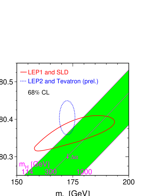
Both the top and masses can be better measured at the LHC and Tevatron. The mass in particular can significantly constrain the triangle, and requires a measurement with a precision on the order of – parts in (of order 10 MeV). The measurement is very sensitive to many details of hadron collisions, including multiple parton interactions in the same collision, multiple hadron interactions in the same crossing, initial state radiation, quark-antiquark parton distribution functions, and QCD backgrounds to leptons and missing transverse energy. At the Tevatron, there is a wealth of experience in understanding the errors associated with this measurement. LHC projections are in the 10 MeV range, but the measurement is of sufficient importance to merit a second measurement with comparable or better sensitivity and completely different systematic uncertainties.
The top mass measurement is competitive at the Tevatron, with the lower cross section being compensated by the benefits of valence quark production close to threshold and hence quieter events. Like the boson mass measurement, this measurement is already systematics dominated. A Tevatron measurement with comparable sensitivity and completely different systematics to the LHC one will give great confidence in this number, as well as improve the precision on it.
Top Mass Measurement
The uncertainty on the top mass measurement is composed of a part which scales with luminosity and a part that does not. The expected improvement of the precision of the top mass measurement is shown in Figure 6.0.75 as a function of integrated luminosity. Recent results from CDF are already more precise than the projections made in the Run IIa Technical Design Report. Further improvements can be expected as we collect more data, with between 4 to 8 of recorded data we can hope to achieve a precision of .
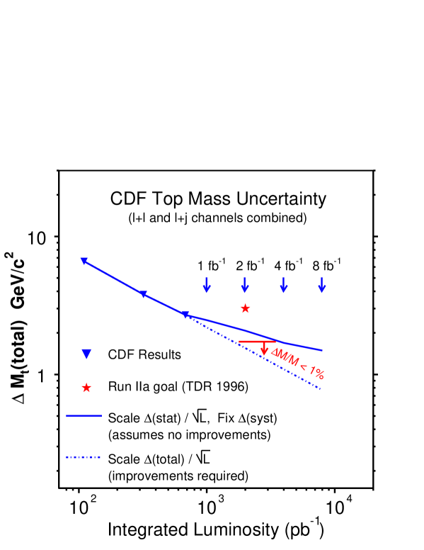
Event selection, in particular the jet thresholds, at the LHC will be quite different from those at the Tevatron. Although both will be using a constrained fit to the mass, they are likely to be sensitive to different types of systematic errors. For example, at the Tevatron, unlike the case at the LHC, there is little or no bias from angular resolution and jet separation, hence it is important to determine the accuracy of the jet kinematics in the Monte Carlo. jet data provides a way to do this test, but it provides low statistics. The expected precision at the LHC is estimated to be between 1.0 GeV [177] and 1.5 GeV [178] which is comparable to what can be achieved at the Tevatron provided sufficient data is collected. The sources of systematic errors at the Tevatron include:
-
•
Jet energy scale: derived from , detector resolution
-
•
Background: systematic uncertainties in modeling the dominant background sources
-
•
-jet modeling: variations in the semi-leptonic branching fraction, fragmentation model, differences in color flow between -jets and light quarks.
-
•
ISR, FSR, UE: tuning of the different models in different Monte Carlo programs
-
•
Method: Fit method, Monte Carlo statistics, and tagging efficiency
-
•
Generator: Differences between PYTHIA or ISAJET and HERWIG when modeling the signal.
The magnitude of the errors are given in Table 6.0.12 together with an estimate of their size assuming the full data set. Further improvements on the precision of the top mass will require more refined modeling and more precise PDF sets.
| Source | Source | ||
|---|---|---|---|
| Jet Energy Scale | 2.5 0.7 | ISR | 0.4 |
| BG shape | 1.1 0.3 | MC statistics | 0.3 0.1 |
| -jet modeling | 0.6 | PDF’s | 0.3 |
| FSR | 0.6 | Generators | 0.2 |
| Method | 0.5 0.2 | -tagging | 0.1 |
Mass Measurement
The total uncertainty on the mass measurement can also be decomposed into a component that scales with luminosity and a part that does not. The uncertainties which scale with luminosity include: statistical uncertainties and systematic uncertainties such as the energy and momentum scale and hadron recoil against . As we collect more data we are able to better calibrate the energy response and reduce the associated uncertainty.
Uncertainties which do not scale with luminosity include: production and decay, PDF’s, the shape of the boson distribution and higher order QCD/QED effects, assumed to be between – MeV. Figure 6.0.76 illustrates the expected improvement in the mass precision as a function of the integrated luminosity. With the full data set at the Tevatron we can expect to measure the mass to a precision of – MeV.141414These error estimates are discussed later. The ultimate precision estimated for the LHC is – MeV. In order to achieve this precision at the LHC, it will require low luminosity running and an excellent understanding of the detector.
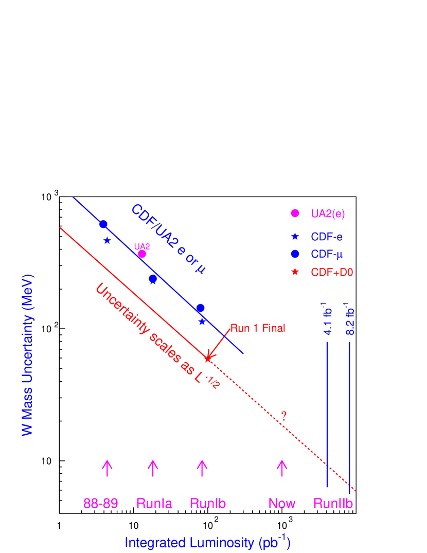
Validation of Standard Model Processes
Modern experimental particle physics relies, more so than in the past, on theoretical predictions, usually in the form of Monte Carlo programs. This is understandable as we evolve from a qualitative to a quantitative understanding of the Standard Model. Validating these tools on high–luminosity, high–energy, hadron–collider data is important, but can be complicated and time–consuming. Current Tevatron data is helping to constrain phenomenological models and to indicate directions for theoretical improvements, but the validation process is limited by data and a lack of appreciation of its importance. By running in an energy regime that is not tainted by (potentially) large contributions of new physics, we can begin to build a complete description of the important Standard Model processes. If our MC tools are not adequate, then analyses at the LHC may rely on background estimates that are imprecise and cannot be easily cross-checked with independent samples. Indications of new physics could potentially be absorbed into “background” distributions, limiting or jeopardizing new physics searches.
An obvious goal for Run II should be the establishment of a “complete” description of Standard Model backgrounds to new physics. To expand beyond our current knowledge, this means obtaining a good understanding of diboson and single top production processes and an excellent understanding of the , jets and multijet processes.
Di-Boson Production
The study of di-boson production at the Tevatron provides complementary tests of the electroweak sector of the Standard Model to those made at LEP. Anomalous pair production of gauge bosons could be an indication of deviations from the Standard Model gauge structure and/or substructure. Anomalous production could manifest itself as an increased production rate or change in the kinematic distributions, such as the gauge boson . The size of anomalous couplings can be used as metrics for evaluating the sensitivity to new physics and characterize any deviation of the and bosons from point particles.
A good understanding of di-boson production is also needed to estimate the background for other important physics. The production of and boson pairs at the Tevatron occurs at a rate of order 100 fb, and constitutes a significant background in searches for the SM Higgs boson or SUSY trilepton signatures. In events when the bosons both decay leptonically, the signature is similar to production with an ISR gluon splitting to a heavy quark pair.
The current status of di-boson production is summarized in Figure 6.0.77. The process is observed with an uncertainty on the cross section measurement that is the theoretical uncertainty [179]. The cross section for processes is bounded above at roughly the Standard Model expectation, which is about the current limit on single top production. With a comparable data set needed to discover single top production, the Tevatron should begin to make quantitative measurements of processes.
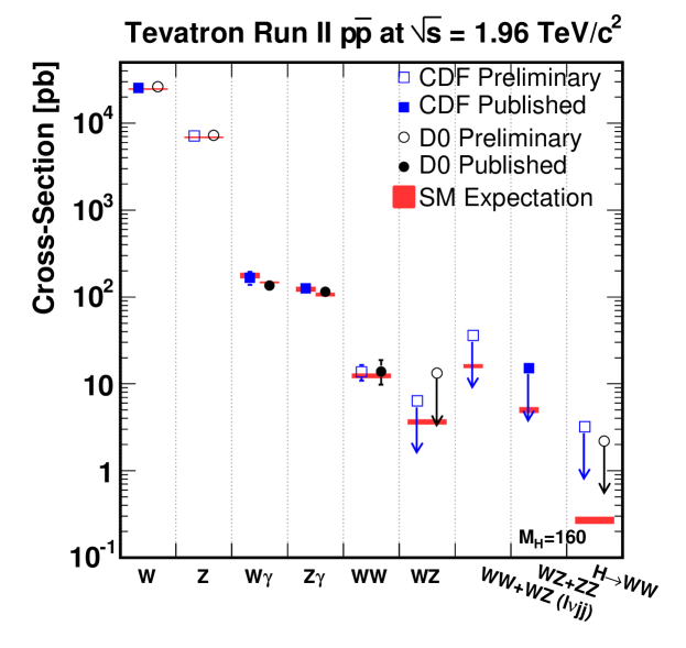
production
While our understanding of inclusive production is quickly becoming systematically–limited, more exclusive topologies involving top are less understood. An important aspect of searches at the LHC is understanding the mass shape of additional jets in events. The rate for such events is roughly a factor smaller than the total rate. Furthermore, the process at the LHC must often be rejected (or selected) with a high efficiency, based on the number of jets in the event. A high–statistics sample of will allow detailed studies of the effect of additional gluon radiation. How often do reconstruction inefficiencies lead to fewer jets than expected? How often does misreconstruction occur, so a jet is formed from calorimeter noise or from underlying event fluctuations? How often does a -tagged jet actually correspond to a quark at the parton level? With thousands of clean, double-tagged top pair events in Run II, we can address all these questions. More support of our understanding of production would be found in the observation of the rapidity asymmetry, which can be observed at a proton-antiproton collider.
Single Top Production
The single top production process has the same signature as the associated production process . Also, since the production rate is proportional to , it probes the top quark width. The SM predictions for the single top cross section are pb for the s–channel process and pb for the t–channel process.
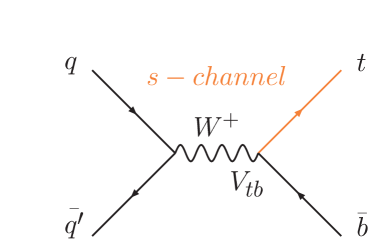
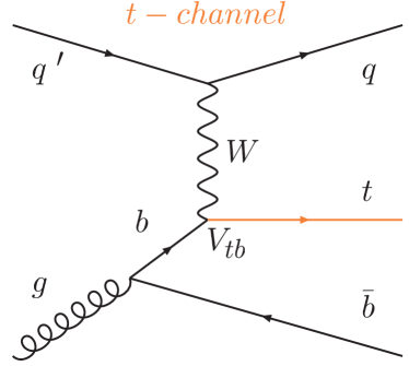
The combined channel likelihood for SM single top production as a function of the integrated luminosity is shown in Figure 6.0.79. With – fb-1 Standard Model single top production will be established, providing an event sample of roughly 75 events. If the measurement is statistically limited, then the total production cross section will be known to roughly 10%. However, a detailed description of kinematic distributions will benefit from increased statistics. It is hard to quantify how well this can be done, but we can estimate that the number of fit quantities is roughly proportional to .151515For a 1-dimensional distribution of say , 10 events are typically needed to obtain a good, Gaussian fit. This can be generalized to many dimensions by picturing 10 slices in each variable. A doubling or quadrupling of the data will easily allow for multi-variate fits, increasing our confidence that we are observing pure Standard Model single top production. As a rule of thumb, we can claim an understanding of a process if we can predict the effect of radiating an extra, energetic jet, which comes with a statistical penalty of 161616This is based on the fact that many electroweak processes receive their dominant corrections at NLO. Observing 15 or 30 single-top-plus-jet events versus only 7 is the difference between Gaussian and Poisson statistics. Further, one expects that cuts can be loosened after discovery, leading to larger and more discriminating datasets.
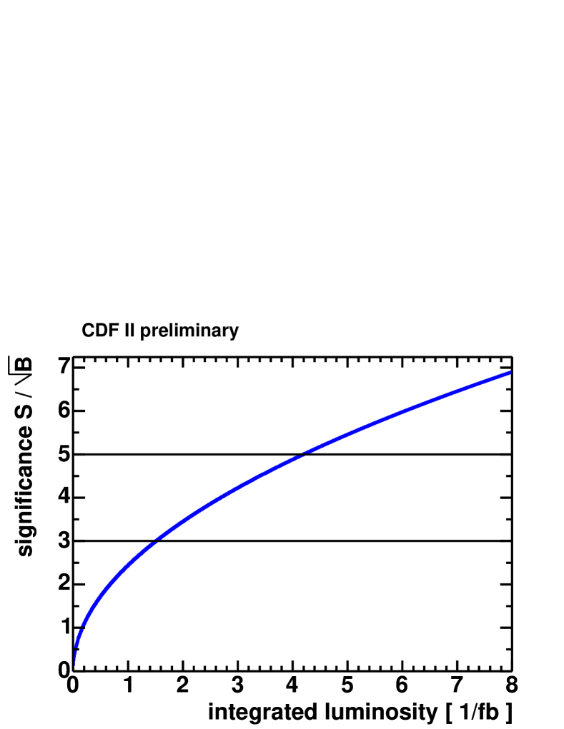
Vector Boson plus Jet Production
or + jets production is a fundamental process that needs to be understood for new physics searches (SUSY and Higgs) at the LHC. We will need to have sensitive tests at lower energy where the effects of new processes do not significantly contribute. Since Vector-Boson + jet is the principle background to top, we need to understand the rate, energy spectrum and correlation between jets in this process.
Since many of the same parton topologies contribute to n jet production at the Tevatron and LHC, Tevatron measurements could be used to normalize the rates using the data to calculate effective –factors. The translation from Tevatron to LHC energies, then, would be a reweighting based on the different contributions of PDF’s. More statistics at the Tevatron could strengthen this extrapolation by providing more jet events.
To further stress the importance of understanding vector boson production, we note that this is a “Standard Candle” process that can be used to determine the proton-proton luminosity. This process has high statistics, can be measured accurately, and is theoretically well understood. At the LHC, the proton-proton luminosity will have to be known to better than 5%. Other techniques to reduce the uncertainty coming from PDF’s involve using cross section ratios which can reduce the overall uncertainty on the luminosity from 5% to 1% [180].
Phenomenological Measurements
Many aspects of our description of the complex structure of hadronic events cannot be addressed from first principles. They are by nature non–perturbative or sufficiently correlated with other aspects of the event to prevent a simple description. Our lack of understanding of these event properties are often the leading systematic uncertainties in analyses. The Tevatron potential for making important PDF measurements is sufficiently rich that we will discuss it separately.
Improving Parton Distribution Functions
Parton Density Functions (PDF’s) are an essential input to the calculation of many hadron-hadron and lepton-hadron production processes. Uncertainties on the PDF’s influence the measurement at several stages in the analysis. The inferred cross section is related to the observed quantities and correction factors through the relation:
PDF’s errors can impact the measurement through the calculation of acceptance (), luminosity (), event selection (), and background estimate ().
The Tevatron and LHC are, borrowing a widely abused term, W/Z factories. The reason that their potential for contributing to the next generation of global QCD analysis (in an analogous fashion to DIS experiments in the last two decades) has not attracted much attention has to do with the fact that the measured cross sections, involving convolutions of two PDF’s, do not depend on the PDF’s in as direct a way as the structure functions of DIS scattering. Thus, it is difficult to highlight which measurement will directly determine which particular features of PDF’s. But, since most of the open issues in current PDF analysis concern sub-dominant effects, the more subtle role to be played by precision data will be both natural and vital. Instead of looking at LO parton formulas for motivation to focus on particular measurements, we now need detailed phenomenological studies of the effects of possible measurements on the remaining uncertainties of PDF’s in the global analysis context, utilizing the new tools developed in recent years, such as the Lagrange multiplier method. Efforts along this line are crucial for the success of the Tevatron and LHC physics programs.
Some of the PDF distributions which are not well constrained include the gluon distribution at high , strange and anti-strange quark content, strange and anti-strange asymmetry, details in the and sector, the ratio and heavy quark distributions. For low , the error on the gluon distribution is expected to be about 3% and increases dramatically for high as shown by the shaded band in Figure 6.0.80.

The following measurements from the Tevatron can be used to help constrain the PDF’s:
-
1.
Inclusive jets at central and forward rapidity,
-
2.
total cross section,
-
3.
Mass,
-
4.
rapidity distributions,
-
5.
forward/backward asymmetry,
-
6.
transverse momentum distributions,
-
7.
charge asymmetry,
-
8.
+ jet cross sections,
-
9.
+ heavy flavor tag cross sections,
-
10.
transverse momentum distributions,
-
11.
top production cross section,
-
12.
direct production cross section.
In the following, we discuss the potential of some of these measurements.
Inclusive Jet Cross Section
Measurement of the inclusive jet cross section is a stringent test of pQCD over many orders of magnitude (see Figure 6.0.81).
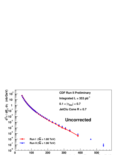
New physics can show up as an excess of events at high compared with pQCD predictions. As is now well-known, high jet production also probes the high gluon distribution, and there is some flexibility in the PDF parameterization which allows it to accommodate some excess at high . Having data at both high and low constrains the fits through the momentum sum rules.
In order to disentangle new physics from PDF effects, one needs to measure jets in the forward region. Figure 6.0.82 shows the increased cross section at high one expects from a quark compositeness model. If data was not available in the forward pseudorapidity region it would be difficult to separate new physics from PDF effects. Inclusive jet cross section results from CDF are shown in Figure 6.0.83 and Figure 6.0.84. Note the different sensitivity to PDF’s from the central region to the forward rapidity regions.

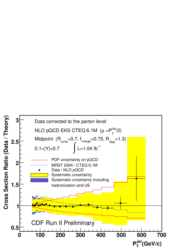
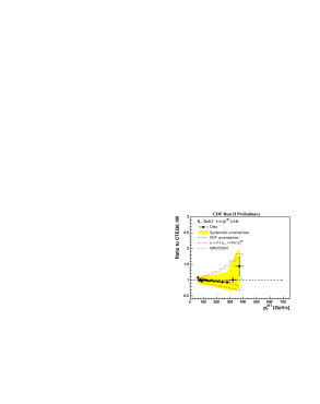
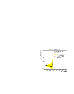
The low transverse energy () region for the inclusive jet production has large errors associated with the uncertainty of jet fragmentation and underlying event. Data from the Tevatron has been used to help understand this region as well. As suggested by the jet figures, the large data set of Run II offers the opportunity for a precision comparison of the Cone (Midpoint) algorithm with the algorithm. These algorithms have differing, and to some extent complementary, strengths and weaknesses. Careful studies of the results from both algorithms applied to the Run II data will allow a detailed understanding of each in preparation for their employment at the LHC.
Precision Measurements, Parton Distribution Uncertainties, the W-mass and Top/Higgs Physics
The differential cross section for production (or, more practically, the cross section for one of the decay leptons in the semi-leptonic decay channel) is sensitive to details of PDF’s. Precise data on these cross sections can play a decisive role in narrowing the uncertainties and clarifying many of the open issues on PDF’s described in the first part of this review. This is because, first, they measure very different combinations of PDF’s compared to DIS experiments, thus provide constraints on many independent quantities not accessible in DIS. (The leptonic asymmetry measured in Run I is a good example.) In addition, the kinematic coverage of the collider cross section data will greatly expand that of available DIS data. It is particularly important that the cross sections be measured as precisely, and in as wide a kinematic range, as is possible at the Tevatron, in order to determine the PDF’s well enough to enable better predictions, hence improved discovery potentials, at the LHC. The impact that the choice of PDF set as well as the treatment of errors has on predictions can be illustrated by the calculations of the cross section at LHC energies summarized in Table 6.0.13.
| PDF Set | (nb) |
|---|---|
| MRST2002 | |
| CTEQ6 | |
| Alekhin02 |
The Alekhin02 fit uses a different subset of data than the MRST and CTEQ PDF’s. This will in general lead to different extrapolations out side of the kinematic region covered by the data used in the fit. The choice of the definition leads to the different error estimate between the calculation using the MRST and CTEQ PDF’s. The data from the Tevatron can help to discriminate between choices of PDF sets.
The transverse momentum distribution of and bosons at the colliders has been the focus of much study, both experimentally and theoretically. The main impetus for this effort has been the desire to achieve the most precise measurement possible of the mass, —a key parameter in precision SM electroweak phenomenology, and hence a potentially powerful indication for new physics. For this purpose, it is critical to reliably quantify the uncertainty of the mass measurement, . But the uncertainty associated with the parton distributions, one of the main contributing factors, is far from well determined. There is no assurance that current estimates (previously mentioned) of – MeV at the Tevatron and – MeV at the LHC are indeed trustworthy.171717For reasons described below, these uncertainties are most likely underestimates.
Historically, estimates of the uncertainty relied heavily on an assumption that correlates it with that of the measured rapidity distribution. More recent studies make use of the uncertainty estimates based on the Hessian basis eigenvector PDF sets, e.g. from CTEQ6. Unfortunately, neither of these approaches contain reliable information on the uncertainties of PDF’s associated with the degrees of freedom in parton parameter space that are most relevant to the mass measurement—the distribution of the vector bosons (or their lepton decay product). In fact, there has been no systematic study so far of the interplay between the distribution of the vector bosons in colliders and the undetermined PDF degrees of freedom.
A fundamental unanswered question is: what degrees of freedom in the parton distribution parameter space are important in determining the distribution of the vector boson and its decay lepton? Of particular interest is the question: are there degrees of freedom that are, so to speak, orthogonal to those that are already well–determined from DIS and -rapidity measurements? It would be remarkable indeed if the degrees of freedom relevant to the distributions are exhausted by those that are already well-constrained by the –inclusive measurements!
Detailed predictions for vector boson distributions are best carried out using a formalism that includes the proper resummation of large logarithm factors of the form (with ). Because the resummation calculation is an involved one, and the parton parameter space is of quite high dimensionality ( 20 or more in conventional global analysis), “intuition” is of very limited value to reach a conclusion on this important issue. We need to incorporate the –resummation calculation into the global QCD analysis, and probe the correlation between parton parameters and measurable distributions in a fully integrated approach. Fortunately, due to recent progress in streamlining the resummation calculation and the global analysis tools, this goal appears to be within reach.
The strategy, when the tools are fully developed, would be:
-
1.
Use the expanded global analysis tools to perform new PDF fits, incorporating existing data on Drell-Yan and distribution data, to explore the impact of these on the determination of parton distribution parameters and their uncertainties (compared to currently existing results).
-
2.
Use the Lagrange Multiplier method (cf. CTEQ papers) to map out the directions in parton parameter space that are particularly sensitive to the distributions; and compare these with the basis eigen-vector directions in current Hessian analysis, as well as those directions closely associated with rapidity distributions.
-
3.
Use the results of the Lagrange Multiplier method to quantify (much more reliably than current methods) the uncertainty of the mass measurement.
-
4.
Use the same results to study the impact on the Higgs search efforts, particularly the associated production channels and , and on single-top production investigations.
-
5.
Reversing the direction of inquiry: ask the question “How can the uncertainties (on mass and and signals) be reduced, if we can improve certain measurements at the Tevatron that can be used as input to the expanded global analysis?” This question can be answered with the same analysis tools by using, for instance, hypothetical goal-oriented data sets. Such studies can provide powerful motivation for refined experimental plans.
The task of carrying out this program is complicated by the fact that resummation calculations introduce certain additional “non-perturbative” parameters of their own. These parameters have been studied before in the context of fixed PDF’s. In the expanded analysis, new efforts are needed to differentiate between these and the PDF parameters whenever possible. The inevitable residual correlations between them then need to be systematically taken into account in the physics applications. The methodology is the same as the case without the factor.
We have highlighted the distribution in the above discussion. The basic idea applies to the full range of possible precision measurements possible at Run II of the Tevatron and the LHC, such as the rapidity and charge asymmetry discussed below. The identification of the most productive measurements requires close collaboration between theorists and experimentalists in an iterative mode, following the strategy outlined above.
Rapidity Distributions
+ jets provides a different constraint on PDF’s when considering semi inclusive final states. + jet production as a function of rapidity is sensitive to PDF’s and differences between LO, NLO and NNLO. It is hard to quantify the luminosity required for this study as it has not yet been attempted with present data. Possibly if the rapidity sensitivity becomes observable at 400 pb-1 (see Figure 6.0.85), then the semi-inclusive sensitivity will require at least 5 as much data.
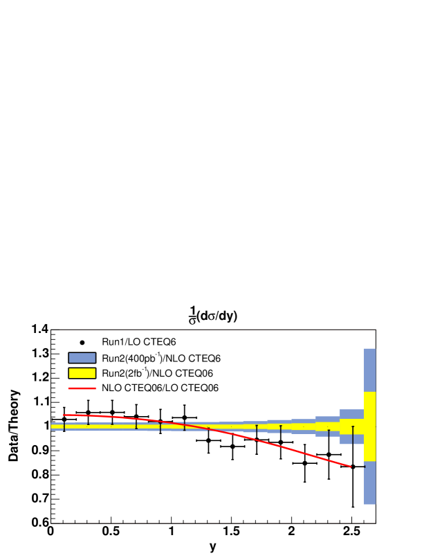
Charge Asymmetry
A measurement of the charge asymmetry constrains the ratio: as . Having more data allows us to explore the lepton dependence of the charge asymmetry. Recent results from CDF are shown in Figure 6.0.86 while data from DØ is shown in Figure 6.0.87 with the error associated with the PDF uncertainty shown as the shaded band. The charge asymmetry is an important input to global QCD fits and can be used to refine PDF’s.
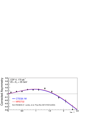
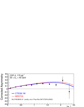
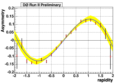
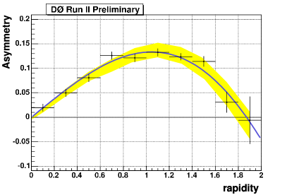
PDF Error Estimates
A significant advance in quantitatively understanding the impact of PDF errors on measurements was the development of new techniques to estimate errors. In the past, an error associated with PDF’s was determined by running Monte Carlo using two different sets and taking the difference. This is clearly not rigorous, since different PDF sets are usually based on different assumptions, include different data sets in the fits, and parameterize the PDF’s differently. However, the practice was carried out for lack of a practical alternative. At the Tevatron, PDF errors can be estimated more quantitatively (see Figure 6.0.88). Consistency between different sets tests the universality of the PDF’s. This is an important cross check of our methodology.
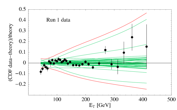
Heavy Flavor PDF’s
There is very little direct experimental input on intrinsic heavy flavor of the proton; all and distributions in existing PDF sets are radiatively generated from the gluons. The heavy flavor content of the proton can be probed through measurements of , and +jet, +jet production via the processes shown in Figure 6.0.89. An understanding of the heavy flavor PDF’s is necessary for precise predictions of Higgs boson production rates. Run II measurements of plus tagged heavy flavor distributions are shown in Figure 6.0.90. Currently, the results are dominated by statistical errors. The largest sources of systematic errors arise from: energy scale, tagging efficiency and the trigger. Single top production in the t-channel process is also sensative to the PDF at high .
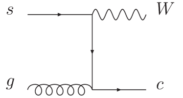
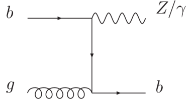
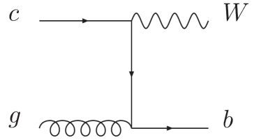

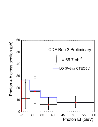
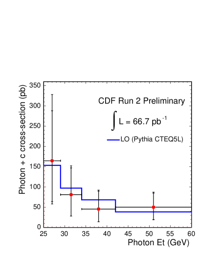
Other Important Phenomenological Measurements
Fragmentation of Quarks and Gluons and the Structure of Jets
Analogous to our exploration of the structure of the proton, the fragmentation of quarks and gluons into hadrons is fundamental science. The large region ( is the fraction of the parton momentum carried by the th hadron) is accessible at the Tevatron, and must be understood to determine how often a “jet” fluctuates into only one observable charged track or photon. This is critical for understanding backgrounds to leptons and photons in Higgs boson final states. Some of the interesting properties of fragmentation that can be studied at the Tevatron are: quark versus gluon jet fragmentation; heavy quark jet fragmentation (, , and even ); the high limit of jet fragmentation for different species of particles; and fragmentation distributions . The Tevatron gives complementary measurements of these quantities for different kinematic slices of and . A particularly interesting and phenomenologically important question is the fraction of gluon and light quark initiated jets that fragment into heavy quarks. A precise determination of this fraction can likely be obtained from a study of the large Run 2 sample of -tagged jet events. At LO this sample has only a negligible contribution from short–distance states and is dominated by b quarks produced in the fragmentation process. Knowledge of this fragmentation process and its associated rates will lead directly to better control of the dominant background for single top production, the backgrounds for measurements of heavy flavor PDF’s and a variety of backgrounds to beyond the Standard Model processes at the LHC.
Details of the Underlying Event
The underlying event (UE) is an unavoidable background to many measurements at the Tevatron and the LHC. There is also interesting QCD physics in the UE since, in general, it contains particles that originated from initial and final state radiation, beam-beam remnants, and multiple parton interactions. CDF has studied the UE in high transverse momentum jet production, but there is still much to be done. In particular, one would like to measure the cross-section for multiple-parton collisions and establish precisely how much it contributes to the UE in various processes. Also, one would like to study the UE in color singlet (e.g. ) production, and compare to the UE in high jet production. CDF can utilize the miniplug and the CLC to extend measurements to large rapidity. Multiplicity distributions in , , Drell Yan, , , and would be very interesting. In the first 200 pb-1, CDF had a clean event (the only one) with 70 associated tracks, 34 in , region, while it had a clean event with zero tracks in that fiducial region (out of 17 events) and almost nothing forward. Such effects are worthy of more study. Certainly the tails of the distribution are sensitive to the UE and possible anomalies. Large fluctuations are presumably due to differences in the impact parameter (an interesting variable). In addition, we should try and establish the rate of vector boson fusion (VBF) and study the probability of rapidity gaps. The following is a list of some of the UE related measurements that need to be completed:
-
1.
The UE in color singlet production (, , photon, Drell Yan, VV, di-photon).
-
2.
The rate of multiple parton collisions.
-
3.
Distributions in the UE (multiplicity, , ).
-
4.
Correlations in the UE.
-
5.
VBF and rapidity gaps.
Heavy Flavor Fragmentation
production and backgrounds to Higgs production have never been satisfactorily understood. In Run I the rate of jet production was larger than expected from theory calculations. A more careful theory calculation was performed using up-to-date information on the fragmentation function and resulted in better agreement [181]. Recent results from CDF are shown in Figure 6.0.91.
Data from the Tevatron will enable us to reduce the systematic uncertainties associated with hadron production. This is important, given the importance of understanding the details of top production at the LHC and the special role of quarks in Higgs boson physics.
Diffractive Physics and Central Exclusive Production
Another section of this report deals more completely with diffraction, as a class of interactions containing large rapidity gaps (typically 4 units) with no hadrons. This implies color singlet exchange, requiring two or more gluons with a (minor) contribution of . This is a frontier of QCD, not fully understood but where much progress has been made through experiments at the Tevatron and HERA. Here we give a brief summary of the two main areas, diffraction and central exclusive production. The latter has become very topical as a possible window on the Higgs sector at the LHC.
Diffraction
Elastic scattering and the total cross section are basic properties of interactions, which will be measured at the LHC by the TOTEM experiment. Unfortunately, they are not very well known at the Tevatron, with three inconsistent () measurements of , and only one measurement of into the Coulomb region and none into the large region beyond 2 GeV2 (interesting from a perturbative point of view). There are no measurements at = 1960 GeV, although the LHC could run at that to make a comparison of and . The Forward Proton Detectors (FPD) of DØ, in a special planned high- run, may make a competitive measurement of and a new measurement of through the dip region GeV2. They should also make some measurements of low mass double pomeron exchange, where means a rapidity gap (no hadrons) and is a completely measured system, e.g. or . This is a potentially rich field, both for studying diffractive mechanisms and for spectroscopy ( is rich in glueball and hybrid states). Single diffractive excitation of low mass and high mass (di-jets, , , heavy flavors) has been measured, but there is a case for a more complete systematic study, e.g. conditional on such massive final states, at different values. From the -dependence at fixed () one could derive a “hard pomeron” trajectory to extrapolate to the LHC. Monte Carlo event generators which have interactions and include diffraction, such as HERWIG [183, 80] and PYTHIA [75] could then be tested and tuned, to improve predictions for the LHC.
Central Exclusive Production
The above mentioned process, , with a simple completely measured state, is called central exclusive production. The possibility that can be a Higgs boson has generated much interest in this process at the LHC. Precise measurements of the scattered primary protons () allow one to measure the Higgs mass with 2 GeV per event, independent of decay mode (e.g. ). The ratio of signal to background can be 1:1, and possibly considerably larger for a MSSM Higgs (in the MSSM the Higgs cross section can be an order of magnitude higher than in the SM). The Higgs quantum numbers can be determined from the azimuthal correlations: proving that is a scalar and has CP= ++ is essential to establishing its identity.
The key question for exclusive central production is what is the cross section? been proposed [148] that has an identical QCD structure, might be measurable at the Tevatron and, if seen, would confirm that must occur and “calibrate” the theory. The Durham group (see e.g. Ref [149, 150, 151]) calculated the cross sections and they have been incorporated into the ExHume [152] generator. The observation of the process in CDF confirms that the exclusive cross section for (SM) 130 GeV is 3 fb or perhaps a factor higher, which is very encouraging. Other exclusive processes which can be related to exclusive production are and
The FP420 R&D collaboration aims to add high precision forward proton detectors to CMS and/or ATLAS. In addition to observations, exclusive central produced by 2-photon exchange should be seen, fb, and final state interactions between the ’s can be studied. Other important 2-photon processes are central and . These have recently been observed in CDF, the first time processes have been seen in hadron-hadron collisions.
Tevatron Experience
Our field is full of new ideas. However, the practicality of those ideas can often only be judged after they have been applied to real data. The Tevatron serves as a proving ground for ideas developed “in shop” and those originating from the LHC perspective.
Measurement Techniques
Systematic uncertainties are difficult to estimate without data in hand. “Rare” effects, such as a jet fragmenting to mostly one leading particle, are nonetheless important when convoluted with the enormous jet cross section. Dedicated studies at the Tevatron continue to improve our understanding of several outstanding experimental issues.
-
•
Rejection rates: The rejection rate for the copious and hard–to–simulate background to photons in hadronic collisions. These are backgrounds to the signal of Higgs boson decay to photon pairs.
-
•
-tagging efficiencies: Determination of -tagging efficiencies in hadronic collisions with many background tracks from other interactions.
-
•
reconstruction efficiencies
Search Strategies
The Tevatron Run II data can be used to validate new and powerful analysis methods, particularly with many of the complications of the LHC environment, at least during the early running. Examples of these methods are:
-
•
Matrix element weighting: The mapping of observed objects back to the “theoretical objects”, with are then weighted according to the fully differential theoretical predictions;
-
•
Neural Network analysis: The disentanglement of (supposedly) complicated correlations between observables based on theoretical training sets of signal and background; and
-
•
Quaero/Sleuth: An algorithm and automated procedure to find deviations from Standard Model predictions and quantify their significance based on the observed data and without the bias of specific new physics scenarios[184].
Other examples are:
-
•
Development of -charge tagging techniques – a useful application for top–mass and –helicity measurements, but an enormous effect on reducing combinatorics in .
-
•
Application of –jet–likelihood methods to separate signal from background.
-
•
Studies of lepton isolation, jet reconstruction, and missing in a hadron collider with many interactions per bunch crossing.
Early or Post– Discovery of New Physics
The design of the LHC provides significant partonic luminosity in the energy range near TeV, and thus the LHC is positioned to discover almost any new phenomena associated with electroweak symmetry breaking. The Tevatron was not designed with this goal in mind, but still has the potential to probe new phenomena up to several hundred GeV. If the last piece of the particle puzzle is a Standard Model Higgs boson, then the Tevatron can probably only provide evidence for its existence in a narrow mass range. However, theoretical arguments suggest this is an unlikely scenario. Almost all alternatives suggest a broad spectrum of new particles and possibly new interactions. The increase in energy from the Tevatron to the LHC is so great the one may be quickly swamped by a full spectrum of new particles. The Tevatron may only be sensitive to the lighter particles of this spectrum, and could provide measurements that are free from other sources of new physics. The Tevatron experiments have proven their capabilities for discovering and studying a heavy new particle (the top), and stand as the center of expertise on the subject. The Tevatron reach for a supersymmetric partner of the top quark with similar mass is documented elsewhere. Certain supersymmetric processes are sensitive to the nature of the lightest superpartner, and there is no compelling study that the LHC can discern a Higgsino from a Wino LSP. The non–observation of certain associated processes (squark or gluino + LSP) at the Tevatron would immediately identify the LSP as a Higgsino. Furthermore, the Tevatron to LHC transition from valence– to gluon–sea dominated partons means that the rates for QCD backgrounds have increased faster than those typical of quark–annihilation processes. The signal–to–background ratio for new light states may be more favorable at the Tevatron, and the systematic errors for searches will be different.
The Health of the Field in the Pre–ILC Data Era
A key consideration in a fore-front field of science is making sure the door is open and inviting to the best and the brightest young scientists starting their careers. If US graduate students stop going into a field due to lack of opportunity for individual initiative and discovery, and the satisfaction of developing and realizing fruits of their ideas, the US strength in many areas will wither before the time to bid on the ILC site.
Responding to the Unexpected
The concurrent running of a mature Tevatron and a developing LHC opens many possibilities. One can easily imagine scenarios in which a discovery (or a non–discovery!) at the LHC would point to complementary measurements at the Tevatron to explore the space of possible theoretical explanations. To study some phenomena, it may be advantageous to have data at a lower–energy, valence–quark– dominated collider in conjunction with a higher–energy, gluon–and–sea–dominated one. One doesn’t know what is unexpected, but some possible examples for which the Tevatron would be critical are:
-
•
The Higgs is discovered, and the LHC measurements of the -- Triangle doesn’t close. Nothing else is seen. Are the LHC top and mass measurements correct?
-
•
An “invisible” particle is observed at the LHC. Is this particle stable, or does it have a small mass splitting with a lighter “invisible” particle that produces soft, but observable decay products?
-
•
A heavy, exotic particle (fractional charge? or a heavy SUSY hadron) is observed at the LHC. Are there lighter exotics that were missed, possibly with lifetimes on the order of the lifetime?
Re–analysis of Tevatron data can be performed after the shutdown of the Tevatron accelerator, provided we are prepared to do so and there is enough data to make it worthwhile. Even if we do not have enough information to find new phenomena now, feedback from the LHC could indicate which channels to study, or how to reduce certain systematic errors. We note that the JADE collaboration has recently performed several interesting QCD analyses despite the fact that the data is over 20 years old!
The Health of the Field: Physicists and Engineers
Jack Steinberger once asked “Why is it that the US produces such wonderful graduate students and builds such lousy (not the actual word) detectors?”. The Tevatron provides opportunities that are very attractive to the best experimental students- playing a central role in world-class measurements, being responsible for entire subsystems, and the opportunities for improvements at the scale of small but first-class groups. The lack of manpower is in many ways an opportunity if handled well- with appropriate support from the Lab and an investment in stream-lining the Tevatron detectors provide positions of responsibility for students and postdocs that will otherwise largely disappear.
A similar situation applies to accelerator physicists and accelerator engineers. Fermilab has a wonderful record of surpassing accelerator goals, dating back to the 400 GeV Main Ring complex, and now happening again with the upgraded Tevatron. 181818The original CDF trigger was designed for a peak luminosity of ; the Tevatron is now running at more than 200 times that. An operating accelerator offers opportunities that are complementary to those of designing a new facility; the LHC upgrade will be very attractive to young accelerator physicists, and having opportunities in the US we believe to be essential to attracting young physicists and engineers into the field.
Additional Capabilities
We should not rule out the prospects of adding new capabilities to the detectors or running at a different center-of-mass energy in order to leverage the experience and facilities at Fermilab. As one example, improving particle identification so that every particle up to a Pt of 20 GeV or so is identified would open up new capabilities unavailable to the LHC detectors. would allow distinguishing the charm-strange quark final state from the up-down quarks in W decay, and could allow distinguishing the b from the b-bar in top pair events, eliminating combinatoric smearing of the top mass. While this could also be done at the LHC, upgrades may be much easier to implement and will provide much more opportunity to youth than at the LHC.
The online event selection is extremely flexible. As we approach the systematic limits of some of the current priority measurements, such as top and mass, one could change the trigger in order to collect more data for measurements which we are not systematics limited. As an example, the physics program would benefit from such a change in priority.
Conclusions
“What are the advantages of running the Tevatron until the end of 2009 and accumulating 8 fb-1 before the LHC has a comparable amount of data?” These include opportunities for measurements and experience that are worthwhile on their own and valuable as input and guidance to LHC analyses. In determining the future of our field, we believe that time is of the essence. Any advantage the Tevatron can give to the LHC physics program allows us to make strategic decisions for the future earlier.
The Tevatron will provide the most precise measurement of the top and mass for many years and will likely remain competitive to what can be achieved at the LHC, provided the Tevatron is not prematurely shut down. The precise measurements will allow for an independent consistency check (with different systematics) of the SM if a Higgs boson is discovered. If the triangle relation does not hold, then the deviation might indicate the energy scale for new physics.
Tevatron data is being used to validate our understanding of physics processes that are important backgrounds to new physics searches, such as , + jets, diboson, single top, and multijet processes. This includes an understanding of cross sections and kinematic distributions. A side–benefit of this measurement program is an improved understanding of QCD Monte-Carlo models. Our physics description of an event requires detailed modeling of effects such as parton showering, fragmentation and hadronization, and the underlying event, which in turn relies on fitting and tuning parton distribution and fragmentation functions.
Many of the uncertainties on the measurements of the physics program at the LHC can only be addressed using data, of which the Tevatron data is the most relevant source. The program of measurements described here draws on the unique talents and expertise of those scientists working on experiments at the Tevatron. We have the opportunity of completing this exciting program at the Tevatron before the LHC has accumulated large amounts of data. The more we learn at the Tevatron now, the more successful the LHC will be.
The decision of when is the right time to stop Tevatron operations needs to take into consideration more than the possibility of discovering new physics. It should also ensure that we utilize fully the Tevatron to strengthen the foundation of our understanding of the Standard Model. There is much interesting and important physics still to be explored. Some measurements would benefit from running longer while others can be done after Tevatron operations stop. It is essential to maintain Fermilab as an interesting place to do physics in order to attract the best graduate students into our field and provide the necessary training for them so as to ensure that the expertise does not dissipate.
References
- [1] Contributed by Peter Skands.
- [2] G. C. Blazey et al., hep-ex/0005012.
- [3] The Snowmass Working Group on Precision Electroweak Measurements, U. Baur et al., eConf C010630, P1WG1 (2001), [hep-ph/0202001].
- [4] S. D. Ellis, Z. Kunszt and D. E. Soper, Phys. Rev. Lett. 69, 1496 (1992).
- [5] S. D. Ellis, Z. Kunszt and D. E. Soper, Phys. Rev. Lett. 64, 2121 (1990).
- [6] S. D. Ellis, Z. Kunszt and D. E. Soper, Phys. Rev. D40, 2188 (1989).
- [7] S. D. Ellis, Z. Kunszt and D. E. Soper, Phys. Rev. Lett. 62, 726 (1989).
- [8] CDF, F. Abe et al., Phys. Rev. D45, 1448 (1992).
- [9] DØ, B. Abbott, M. Bhattacharjee, D. Elvira, F. Nang and H. Weerts, FERMILAB-PUB-97-242-E.
- [10] CDF, F. Abe et al., Phys. Rev. Lett. 68, 1104 (1992).
- [11] CDF, F. Abe et al., Phys. Rev. Lett. 70, 713 (1993).
- [12] S. D. Ellis, Z. Kunszt and D. E. Soper, Phys. Rev. Lett. 69, 3615 (1992), [hep-ph/9208249].
- [13] M. H. Seymour, Nucl. Phys. B513, 269 (1998), [hep-ph/9707338].
- [14] CDF, F. Abe et al., Phys. Rev. D45, 1448 (1992).
- [15] S. D. Ellis, J. Huston and M. Tonnesmann, eConf C010630, P513 (2001), [hep-ph/0111434].
- [16] Special thanks are due M. Wobisch and G. Salam for pursuing this issue with great energy.
- [17] S. D. Ellis and D. E. Soper, Phys. Rev. D48, 3160 (1993), [hep-ph/9305266].
- [18] S. Catani, Y. L. Dokshitzer and B. R. Webber, Phys. Lett. B285, 291 (1992).
- [19] S. Catani, Y. L. Dokshitzer, M. H. Seymour and B. R. Webber, Nucl. Phys. B406, 187 (1993).
- [20] DØ, V. M. Abazov et al., Phys. Lett. B525, 211 (2002), [hep-ex/0109041].
- [21] M. Cacciari and G. P. Salam, hep-ph/0512210.
- [22] http://hepforge.cedar.ac.uk/ktjet/.
- [23] CDF, A. Abulencia et al., hep-ex/0512020.
- [24] M. Voutilainen, proceedings of the DIS2006 workshop , [hep-ex/0609026].
- [25] CDF, R. Field, AIP Conf. Proc. 828, 163 (2006).
- [26] CDF, A. Abulencia et al., Phys. Rev. Lett. 96, 122001 (2006), [hep-ex/0512062].
- [27] CDF, D. Acosta et al., hep-ex/0505013.
- [28] Taken from the Ph.D. thesis of M. Tönnesmann, under (intense) preparation.
- [29] S. Frixione and B. R. Webber, hep-ph/0207182.
- [30] S. Frixione, P. Nason and B. R. Webber, JHEP 08, 007 (2003), [hep-ph/0305252].
- [31] S. Frixione, E. Laenen, P. Motylinski and B. R. Webber, hep-ph/0512250.
- [32] S. Frixione and B. R. Webber, hep-ph/0601192.
- [33] G. Sterman, hep-ph/0501270.
- [34] Y. L. Dokshitzer and G. Marchesini, JHEP 01, 007 (2006), [hep-ph/0509078].
- [35] A. Banfi, G. P. Salam and G. Zanderighi, JHEP 08, 062 (2004), [hep-ph/0407287].
- [36] R. B. Appleby and M. H. Seymour, JHEP 09, 056 (2003), [hep-ph/0308086].
- [37] C. F. Berger et al., eConf C010630, P512 (2001), [hep-ph/0202207].
- [38] J. Baines et al., hep-ph/0601164.
- [39] U. Karshon, I. Schienbein and P. Thompson, hep-ph/0608118.
- [40] W.-K. Tung, AIP Conf. Proc. 753, 15 (2005), [hep-ph/0410139].
- [41] J. C. Collins and W.-K. Tung, Nucl. Phys. B278, 934 (1986).
- [42] M. A. G. Aivazis, J. C. Collins, F. I. Olness and W.-K. Tung, Phys. Rev. D50, 3102 (1994), [hep-ph/9312319].
- [43] J. C. Collins, Phys. Rev. D58, 094002 (1998), [hep-ph/9806259].
- [44] J. C. Collins, F. Wilczek and A. Zee, Phys. Rev. D18, 242 (1978).
- [45] W.-K. Tung, Proceedings of 14th International Workshop on Deep Inelastic Scattering (DIS 2006), Tsukuba, Japan (2006).
- [46] R. S. Thorne, Proceedings of 14th International Workshop on Deep Inelastic Scattering (DIS 2006), Tsukuba, Japan (2006).
- [47] S. J. Brodsky, P. Hoyer, C. Peterson and N. Sakai, Phys. Lett. B93, 451 (1980).
- [48] S. J. Brodsky, C. Peterson and N. Sakai, Phys. Rev. D23, 2745 (1981).
- [49] CDF, A. Abulencia et al., Phys. Rev. D74, 032008 (2006).
- [50] CDF, D. Acosta et al., Phys. Rev. D71, 012005 (2005), [hep-ex/0410058].
- [51] R. S. Thorne, Phys. Rev. D73, 054019 (2006), [hep-ph/0601245].
- [52] M. A. G. Aivazis, F. I. Olness and W.-K. Tung, Phys. Rev. D50, 3085 (1994), [hep-ph/9312318].
- [53] J. Pumplin et al., JHEP 0207, 012 (2002), [hep-ph/0201195].
- [54] A. Chuvakin and J. Smith, Comput. Phys. Commun. 143, 257 (2002), [hep-ph/0103177].
- [55] F. I. Olness and R. J. Scalise, Phys. Rev. D57, 241 (1998), [hep-ph/9707459].
- [56] M. Kramer, F. I. Olness and D. E. Soper, Phys. Rev. D62, 096007 (2000), [hep-ph/0003035].
- [57] W. Giele et al., hep-ph/0204316.
- [58] M. Dittmar et al., hep-ph/0511119.
- [59] M. Buza, Y. Matiounine, J. Smith, R. Migneron and W. L. van Neerven, Nucl. Phys. B472, 611 (1996), [hep-ph/9601302].
- [60] B. Mele and P. Nason, Phys. Lett. B245, 635 (1990).
- [61] Particle Data Group, S. Eidelman et al., Phys. Lett. B592, 1 (2004).
- [62] W. Bernreuther and W. Wetzel, Nucl. Phys. B197, 228 (1982).
- [63] W. Bernreuther, Ann. Phys. 151, 127 (1983).
- [64] S. A. Larin, T. van Ritbergen and J. A. M. Vermaseren, Nucl. Phys. B438, 278 (1995), [hep-ph/9411260].
- [65] K. G. Chetyrkin, B. A. Kniehl and M. Steinhauser, Phys. Rev. Lett. 79, 2184 (1997), [hep-ph/9706430].
- [66] F. I. Olness, R. J. Scalise and W.-K. Tung, Phys. Rev. D59, 014506 (1999), [hep-ph/9712494].
- [67] E. Laenen, S. Riemersma, J. Smith and W. L. van Neerven, Nucl. Phys. B392, 162 (1993).
- [68] M. Buza, Y. Matiounine, J. Smith and W. L. van Neerven, Phys. Lett. B411, 211 (1997), [hep-ph/9707263].
- [69] M. Buza, Y. Matiounine, J. Smith and W. L. van Neerven, Eur. Phys. J. C1, 301 (1998), [hep-ph/9612398].
- [70] Y. Matiounine, J. Smith and W. L. van Neerven, Phys. Rev. D57, 6701 (1998), [hep-ph/9801224].
- [71] A. Chuvakin, J. Smith and W. L. van Neerven, Phys. Rev. D62, 036004 (2000), [hep-ph/0002011].
- [72] A. Chuvakin, J. Smith and W. L. van Neerven, Phys. Rev. D61, 096004 (2000), [hep-ph/9910250].
- [73] A. Vogt, Comput. Phys. Commun. 170, 65 (2005), [hep-ph/0408244].
- [74] J. Huston, PDF Weight Method.
- [75] T. Sjostrand, L. Lonnblad, S. Mrenna and P. Skands, hep-ph/0308153.
- [76] H. Plothow-Besch, Comput. Phys. Commun. 75, 396 (1993).
- [77] D. Bourilkov, hep-ph/0305126.
- [78] M. R. Whalley, D. Bourilkov and R. C. Group, hep-ph/0508110.
- [79] D. Bourilkov, R. C. Group and M. R. Whalley, hep-ph/0605240.
- [80] G. Corcella et al., hep-ph/0210213.
- [81] W. T. Giele, S. A. Keller and D. A. Kosower, hep-ph/0104052.
- [82] J. Pumplin et al., Phys. Rev. D65, 014013 (2002), [hep-ph/0101032].
- [83] P. M. Nadolsky and Z. Sullivan, eConf C010630, P510 (2001), [hep-ph/0110378].
- [84] S. Gieseke, JHEP 01, 058 (2005), [hep-ph/0412342].
- [85] H1, C. Adloff et al., Eur. Phys. J. C19, 289 (2001), [hep-ex/0010054].
- [86] ZEUS, S. Chekanov et al., Eur. Phys. J. C23, 615 (2002), [hep-ex/0112029].
- [87] ZEUS, S. Chekanov et al., Phys. Lett. B547, 164 (2002), [hep-ex/0208037].
- [88] ZEUS, S. Chekanov et al., Eur. Phys. J. C42, 1 (2005), [hep-ph/0503274].
- [89] S. Alekhin, JETP Lett. 82, 628 (2005), [hep-ph/0508248].
- [90] A. D. Martin, R. G. Roberts, W. J. Stirling and R. S. Thorne, Phys. Lett. B604, 61 (2004), [hep-ph/0410230].
- [91] J. Pumplin, D. R. Stump and W. K. Tung, Phys. Rev. D65, 014011 (2002), [hep-ph/0008191].
- [92] C. Pascaud and F. Zomer, LAL-94-42.
- [93] G. Lobo, Prepared for Workshop on Future Physics at HERA (Preceded by meetings 25-26 Sep 1995 and 7-9 Feb 1996 at DESY), Hamburg, Germany, 30-31 May 1996.
- [94] D. Graudenz, M. Hampel, A. Vogt and C. Berger, Z. Phys. C70, 77 (1996), [hep-ph/9506333].
- [95] D. A. Kosower, Nucl. Phys. B520, 263 (1998), [hep-ph/9708392].
- [96] M. Wobisch, DESY-THESIS-2000-049.
- [97] T. Carli, G. P. Salam and F. Siegert, hep-ph/0510324.
- [98] T. Kluge, K. Rabbertz and M. Wobisch, in preparation, see http://hepforge.cedar.ac.uk/fastnlo/ .
- [99] Z. Nagy, Phys. Rev. D68, 094002 (2003), [hep-ph/0307268].
- [100] Z. Nagy, Phys. Rev. Lett. 88, 122003 (2002), [hep-ph/0110315].
- [101] N. Kidonakis and J. F. Owens, Phys. Rev. D63, 054019 (2001), [hep-ph/0007268].
- [102] CMS Collaboration, CERN-LHCC-2006-021.
- [103] T. Sjostrand, S. Mrenna and P. Skands, JHEP 05, 026 (2006), [hep-ph/0603175].
- [104] CDF, T. Affolder et al., Phys. Rev. D65, 092002 (2002).
- [105] R. Field and R. C. Group, hep-ph/0510198.
- [106] R. F. Field, Pythia tunes A, B, C, and D, private communication.
- [107] CDF, R. Field, Acta Phys. Polon. B36, 167 (2005).
- [108] DØ, V. M. Abazov et al., Phys. Rev. Lett. 94, 221801 (2005), [hep-ex/0409040].
- [109] A. Banfi, G. P. Salam and G. Zanderighi, JHEP 03, 073 (2005), [hep-ph/0407286].
- [110] G. C. Blazey, Prepared for Physics at Run II: QCD and Weak Boson Physics Workshop: Final General Meeting, Batavia, Illinois, 4-6 Nov 1999; see section 3.5.
- [111] S. Mrenna and P. Richardson, JHEP 05, 040 (2004), [hep-ph/0312274].
- [112] S. Hoche et al., hep-ph/0602031.
- [113] M. L. Mangano, M. Moretti, F. Piccinini, R. Pittau and A. D. Polosa, JHEP 07, 001 (2003), [hep-ph/0206293].
- [114] T. Gleisberg et al., JHEP 02, 056 (2004), [hep-ph/0311263].
- [115] A. Schälicke and F. Krauss, JHEP 07, 018 (2005).
- [116] M. Begel, T. Gleisberg and M. Zielinski, hep-ex/0602019, M. Begel, talk at the TeV4LHC workshop meeting, BNL, 3-5 February (2005), T. Gleisberg, talk at the TeV4LHC workshop meeting, CERN, 28-30 April (2005), M. Zielinski, proceedings of “Particles and Nuclei International Conference” (PANIC 05), arXiv:hep-ex/0602019.
- [117] CDF, D. Acosta et al., Phys. Rev. D70, 072002 (2004), [hep-ex/0404004].
- [118] CDF, F. Abe et al., Phys. Rev. Lett. 67, 2937 (1991).
- [119] DØ, V. M. Abazov et al., Phys. Rev. Lett. 94, 221801 (2005), [hep-ex/0409040].
- [120] K. Goulianos, hep-ph/0407035.
- [121] K. Goulianos, Nucl. Phys. Proc. Suppl. 146, 166 (2005).
- [122] K. Goulianos, Phys. Rept. 101, 169 (1983).
- [123] CDF, F. Abe et al., Phys. Rev. D50, 5535 (1994).
- [124] K. Goulianos and J. Montanha, Phys. Rev. D59, 114017 (1999), [hep-ph/9805496].
- [125] K. Goulianos, Phys. Lett. B358, 379 (1995).
- [126] K. Goulianos, hep-ph/0203141.
- [127] E. Levin, hep-ph/9808486.
- [128] J. C. Collins, J. Phys. G28, 1069 (2002), [hep-ph/0107252].
- [129] The H1 Collaboration, F. P. Schilling, hep-ex/0210027.
- [130] C. Royon, Mod. Phys. Lett. A18, 2169 (2003), [hep-ph/0308283].
- [131] M. Boonekamp, R. Peschanski and C. Royon, Phys. Rev. Lett. 87, 251806 (2001), [hep-ph/0107113].
- [132] M. Boonekamp, R. Peschanski and C. Royon, Nucl. Phys. B669, 277 (2003), [hep-ph/0301244].
- [133] A. Bialas and P. V. Landshoff, Phys. Lett. B256, 540 (1991).
- [134] A. Donnachie and P. V. Landshoff, Phys. Lett. B296, 227 (1992), [hep-ph/9209205].
- [135] A. Kupco, C. Royon and R. Peschanski, Phys. Lett. B606, 139 (2005), [hep-ph/0407222].
- [136] M. Boonekamp, R. Peschanski and C. Royon, Phys. Lett. B598, 243 (2004), [hep-ph/0406061].
- [137] H1, C. Adloff et al., Z. Phys. C76, 613 (1997), [hep-ex/9708016].
- [138] R. Peschanski, C. Royon, E. Sauvan and L. Schoeffel, in preparation.
- [139] C. Royon, L. Schoeffel, J. Bartels, H. Jung and R. Peschanski, Phys. Rev. D63, 074004 (2001), [hep-ph/0010015].
- [140] J. Kalliopuska et al., HIP-2003-11/EXP .
- [141] M. Boonekamp, J. Cammin, R. Peschanski and C. Royon, hep-ph/0504199.
- [142] M. Boonekamp, J. Cammin, S. Lavignac, R. Peschanski and C. Royon, Phys. Rev. D73, 115011 (2006), [hep-ph/0506275].
- [143] M. Boonekamp, R. Peschanski, C. Royon and L. Schoeffel, in preparation, 2006.
- [144] DØ, Proposal P-900 to FERMILAB PAC .
- [145] A. Edin, G. Ingelman and J. Rathsman, Phys. Lett. B366, 371 (1996).
- [146] B. E. Cox and J. R. Forshaw, Comput. Phys. Commun. 144, 104 (2002), [hep-ph/0010303].
- [147] R. Appleby et al., http://www.fp420.com.
- [148] M. G. Albrow et al., hep-ex/0511057.
- [149] A. B. Kaidalov, V. A. Khoze, A. D. Martin and M. G. Ryskin, Eur. Phys. J. C33, 261 (2004), [hep-ph/0311023].
- [150] V. A. Khoze, A. D. Martin, M. G. Ryskin and W. J. Stirling, Eur. Phys. J. C38, 475 (2005), [hep-ph/0409037].
- [151] J. R. Forshaw, hep-ph/0508274.
- [152] J. Monk and A. Pilkington, hep-ph/0502077.
- [153] M.G.Albrow and A.Hamilton, Workshop on Forward Physics at the LHC (Manchester), http://www.fp420.com/conference/.
- [154] M. G. Albrow and A. Rostovtsev, hep-ph/0009336.
- [155] V. A. Khoze, A. D. Martin and M. G. Ryskin, Eur. Phys. J. C24, 581 (2002), [hep-ph/0203122].
- [156] B. E. Cox et al., Eur. Phys. J. C45, 401 (2006), [hep-ph/0505240].
- [157] V. A. Khoze, A. D. Martin and M. G. Ryskin, Eur. Phys. J. C34, 327 (2004), [hep-ph/0401078].
- [158] J. R. Ellis, J. S. Lee and A. Pilaftsis, Phys. Rev. D71, 075007 (2005), [hep-ph/0502251].
- [159] K.Goulianos, presentation, these proceedings.
- [160] A. R. White, hep-ph/0510034.
- [161] A. R. White, Phys. Rev. D72, 036007 (2005), [hep-ph/0412062].
- [162] B. E. Cox and A. Pilkington, Phys. Rev. D72, 094024 (2005), [hep-ph/0508249].
- [163] M. Boonekamp and T. Kucs, Comput. Phys. Commun. 167, 217 (2005), [hep-ph/0312273].
- [164] V. A. Khoze, A. D. Martin and M. G. Ryskin, Paper in preparation.
- [165] The TOTEM Collaboration, R. Orava et al., Technical design report. Total cross section, elastic scattering and diffraction dissociation at the Large Hadron Collider at CERN, CERN-LHCC-2004-002.
- [166] The CMS Collaboration, Expression of Interest for Diffractive Physics, CERN-LHCC-2004-003/G-068, 2004.
- [167] The ATLAS Collaboration, ATLAS forward detectors for luminosity measurement and monitoring, CERN-LHCC-2004-010, LHCC I-014, 2004.
- [168] M. G. Albrow et al., CERN-LHCC-2005-025.
- [169] A. De Roeck, V. A. Khoze, A. D. Martin, R. Orava and M. G. Ryskin, Eur. Phys. J. C25, 391 (2002), [hep-ph/0207042].
- [170] S. Alekhin et al., hep-ph/0601013.
- [171] A. V. Kisselev, V. A. Petrov and R. A. Ryutin, Phys. Lett. B630, 100 (2005), [hep-ph/0506034].
- [172] R. Engel, talk, Xth Blois Workshop on Elastic and Diffractive Scattering, Helsinki, Finland, 2003.
- [173] P. M. Weilbacher, P. A. Duc and U. Fritze von Alvensleben, Astron. Astrophys. 397, 545 (2003), [astro-ph/0210393].
- [174] TOTEM, M. Deile et al., hep-ex/0602021.
- [175] D. McGinnis, Machine Status and Performance Projections, Presentation to P5, 2006.
- [176] ALEPH, DELPHI, L3 and OPAL Collaborations, and the LEP Electroweak Working Group, hep-ex/0511027.
- [177] I. Borjanovic et al., Eur. Phys. J. C39S2, 63 (2005), [hep-ex/0403021].
- [178] S. Heinemeyer, W. Hollik and G. Weiglein, Phys. Rept. 425, 265 (2006), [hep-ph/0412214].
- [179] J. M. Campbell and R. K. Ellis, Phys. Rev. D62, 114012 (2000), [hep-ph/0006304].
- [180] M. Dittmar, F. Pauss and D. Zurcher, Phys. Rev. D56, 7284 (1997), [hep-ex/9705004].
- [181] M. Cacciari and P. Nason, Phys. Rev. Lett. 89, 122003 (2002), [hep-ph/0204025].
- [182] M. D’Onofrio, CDF/PUB/JET/PUBLIC/8418.
- [183] G. Corcella et al., JHEP 01, 010 (2001), [hep-ph/0011363].
- [184] B. Knuteson, eConf C0303241, TULT001 (2003), [hep-ex/0305065].