Perturbation theory and non-perturbative renormalization flow
in scalar field theory at finite temperature

Abstract

We use the non-perturbative renormalization group to clarify some features of perturbation theory in thermal field theory. For the specific case of the scalar field theory with $O(N)$ symmetry, we solve the flow equations within the local potential approximation. This approximation reproduces the perturbative results for the screening mass and the pressure up to order $g^{3}$, and starts to differ at order $g^{4}$. The method allows a smooth extrapolation to the regime where the coupling is not small, very similar to that obtained from a simple self-consistent approximation.

I Introduction

Perturbative calculations at high temperature suffer from bad convergent behavior. Even the thermodynamical quantities, such as the pressure or the entropy density, which are dominated by short wavelength degrees of freedom – for which one could expect perturbation theory to be reasonably good – are not well described by a strict expansion in powers of the coupling constant. This problem has been particularly studied in quantum chromodynamics, in the context of the quark-gluon plasma (for a recent review, see Blaizot et al. (2003a)). In this case, the perturbative expansion of the thermodynamic potential is known up to order $g^{6}\log g$, where $g$ is the gauge coupling Arnold and Zhai (1995); Zhai and Kastening (1995); Braaten and Nieto (1996); Kajantie et al. (2003) (the $g^{6}$ term requires non-perturbative methods Di Renzo et al. (2006)). However, the problem is not specific to QCD at high temperature: Similar poor convergence behavior appears also in the simpler scalar field theory Parwani and Singh (1995), and has also been observed in the case of large-$N$ $\phi^{4}$ theory Drummond et al. (1998).

Reorganizations of the perturbative expansion, based on various arguments, have been proposed in order to extend the usefulness of weak coupling calculations to regimes of not too small coupling. These involve “screened perturbation theory” Karsch et al. (1997), “hard thermal loop perturbation theory” Andersen et al. (2001, 1999, 2002, 2004); Andersen and Strickland (2005), and the approach put forward in Refs. Blaizot et al. (1999a, b); Blaizot et al. (2001), based on an expansion of the thermodynamical potential in terms of dressed propagators which involve two-particle irreducible (2PI) diagrams Luttinger and Ward (1960); Baym (1962); Cornwall et al. (1974). The approach of Blaizot et al. (1999a, b); Blaizot et al. (2001) exploits a nonperturbative expression for the entropy density that can be obtained from a $\Phi$-derivable two-loop approximation Vanderheyden and Baym (1998). Here the emphasis is on a physical picture involving quasiparticles whose residual interactions are assumed to be weak after the bulk of the interaction effects have been incorporated in the spectral properties of these quasiparticles. It has been shown in particular that the entropy density of the quark gluon plasma can be well understood within such a scheme down to temperatures $T\gtrsim 3T_{c}$ where the coupling can be as large as $g\approx 2$ Blaizot et al. (2001). As an alternative to resummations, effective field theories have also been used Braaten and Nieto (1996). Among those, dimensional reduction, which emphasizes the role of the zero Matsubara frequency, stands out as a very powerful one Kajantie et al. (2001); Braaten and Nieto (1995). An interesting feature of the perturbative calculations when organized through the dimensionally reduced effective theory is that the large scale dependence of strict perturbation theory is considerably reduced when the effective parameters are not subsequently expanded out Kajantie et al. (2003); Blaizot et al. (2003b). When this is done, the predictions of dimensional reduction become similar to those of the 2PI resummation.

In fact, the origin of the difficulties of thermal perturbation theory is now well understood. What complicates the situation is the fact that the coupling constant alone does not control the magnitude of corrections to the free theory: Thermal fluctuations of various wavelengths play also an essential role. In the weak coupling regime, the thermal system is characterized by a hierarchy of scales: Most particles have momenta of the order of the temperature. At high temperature, these “hard” degrees of freedom dominate the thermodynamics and their interactions are accurately described by ordinary perturbation theory. However, perturbative corrections to the thermodynamical functions involve also “soft” degrees of freedom, whose momenta are typically of order $gT$. These soft modes are non-perturbatively related by their coupling to the hard modes. Such corrections are easily handled by resummations or effective theories. Furthermore, the soft modes also interact among themselves. Although perturbative, these interactions generate corrections which take the form of an expansion in powers of $g$ rather than of $g^{2}$ as is the case for ordinary perturbation theory: as a result, perturbation theory becomes less accurate. In QCD, there exists a further scale, $g^{2}T$ for which perturbation theory stops to make sense: at this scale, the self interactions of the modes become comparable to their kinetic energies, invalidating any expansion around free particle motion. The problems associated with this “ultra-soft” scale are specific to non-abelian gauge theories; they will not be discussed in this paper.

There are indications, already alluded to above, that the structure identified in weak coupling, which is based on the hierarchy of scales that we have just discussed, seem to survive, after appropriate resummation, or appropriate use of effective theories, even in regimes of strong coupling where the arguments used to identify the structure become unjustified. That is, the resummations that have been motivated by analyzing the weak coupling regime, provide a smooth extrapolation into the regime of strong coupling where a strict expansion in powers of the coupling does not make sense. The purpose of this paper is to shed light on this issue by using the non-perturbative renormalization group (NPRG) Wetterich (1993); Ellwanger (1993); Tetradis and Wetterich (1994); Morris (1994a, b).

There is some analogy between the effective field theory approach and the NPRG: in effective field theory one integrates out degrees of freedom above some cut-off; in the renormalization group this integration is done smoothly. In a sense, the renormalization group builds up a continuous tower of effective theories that lie infinitely close to each other and are labeled by a momentum cut-off scale $\kappa$. These effective theories are related by a renormalization group flow equation. The picture remains essentially the same for any value of the coupling.

The NPRG has been applied, in various incarnations (it is also called exact, or functional), to a variety of problems in condensed matter Delamotte et al. (2004); Delamotte and Canet (2005), in particle Ellwanger (1994); Ellwanger and Wetterich (1994); Ellwanger et al. (1998); Pawlowski et al. (2004); Fischer and Gies (2004); Arnone et al. (2005); Morris and Rosten (2006) and nuclear physics (for reviews see Bagnuls and Bervillier (2001); Berges et al. (2002); Pawlowski (2005)). It has been applied to problems at finite temperature Tetradis and Wetterich (1994); Reuter et al. (1993); Andersen and Strickland (1999); D’Attanasio and Pietroni (1996); Liao and Strickland (1995); Braun et al. (2004), and the general behaviors that we shall report in this paper have been known already for some time. However, the main focus of previous studies has been the description of the phase transitions, rather than the specific problem that we want to address here.

The outline of this paper is as follows. In Sec. II, we present a brief review of available results concerning perturbation theory for a scalar field with $O(N)$ symmetry. We also discuss a simple self-consistent $\Phi$-derivable approximation that becomes exact in the large $N$ limit. Section III gives a brief introduction to the non-perturbative renormalization group and the local potential approximation. Specific features of finite temperature calculations are recalled. In particular we introduce a regulator that we found particularly convenient for such calculations. In Sec. IV we integrate the flow equations numerically and discuss the results obtained. Finally, in Section V, we perform a perturbative analysis of the flow equations and comment the results. Note that a preliminary account of this work was presented in Refs. Blaizot (2006a, b).

II Perturbation theory and the need for resummation

In this section we briefly review existing results of perturbation theory for the thermodynamics of the scalar field. We also recall how a simple self-consistent approximation based on the lowest oder 2PI diagram, can be used to include non perturbative effects that allow for a smooth extrapolation to strong coupling. This will be useful later in our discussion, as it turns out that the results of this self-consistent approximation are close to those of the non-perturbative RG within the local potential approximation.

II.1 Brief review of results from perturbation theory

We consider a scalar $\phi^{4}$ theory in $d$ dimensions, defined by the $O(N)$ symmetric Lagrangian

$$\mathcal{L}(x)=\frac{1}{2}\left[\partial\varphi(x)\right]^{2}-\frac{1}{2}m^{2}\varphi^{2}(x)-g^{2}\left[\varphi^{2}(x)\right]^{2},$$ (1)

where the field $\varphi(x)$ has $N$ real components $\varphi_{i}(x)$, with $i=1,...,N$. The temperature $T$ ($\beta=1/T$) enters through the action

$$S=\int_{0}^{\beta}d\tau\int d^{d-1}x\,\mathcal{L}(x),$$ (2)

and the periodicity of the fields in imaginary time, $\varphi(\beta)=\varphi(0)$. We shall fix the bare parameters of the action at $T=0$, in order to have a vanishing renormalized mass and a given value of the renormalized coupling constant (the last point is discussed in Sec. II.2). Then we turn on the temperature at a given fixed value and we study the finite temperature predictions of the model for various values of the zero-temperature coupling.

There are two physical quantities that we shall discuss in this paper: the screening mass, and the pressure.

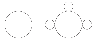
Figure 1: Diagrams that contribute to the screening mass $m_{D}^{2}$ at order $g^{2}$ (left) and at order $g^{3}$ (right).

Up to order $g^{4}$, the screening mass reads Braaten and Nieto (1995):

$$\!\!m_{D}^{2}=g^{2}T^{2}\Big{\{}1-3\frac{g}{\pi}-\frac{9}{2}\left[\ln{\bar{\mu}\over 2\pi T}-{4\over 3}\ln{g\over\pi}-2.415\right]\!\left(\frac{g}{\pi}\right)^{2}+{\mathcal{O}}(g^{3})\Big{\}},$$ (3)

where $\bar{\mu}^{2}=4\pi e^{-\gamma}\mu^{2}$ with $\mu^{2}$ the scale introduced in dimensional regularization, $\gamma$ the Euler constant, and here $g^{2}=g^{2}(\bar{\mu})$ is the $\overline{\rm MS}$ coupling constant at the renormalization scale $\bar{\mu}$. Similarly, the weak–coupling expansion of the pressure has been computed (in the massless case) to order $g^{5}$, and reads Arnold and Zhai (1994); Parwani and Singh (1995); Braaten and Nieto (1995):

$$P = P_{0}\Bigg{[}1-{15\over 8}\left(\frac{g}{\pi}\right)^{2}+{15\over 2}\left(\frac{g}{\pi}\right)^{3}+{135\over 16}\left(\log{\bar{\mu}\over 2\pi T}+0.4046\right)\left(\frac{g}{\pi}\right)^{4}$$ (4)

$$\quad-{405\over 8}\left(\log{\bar{\mu}\over 2\pi T}-{4\over 3}\log\frac{g}{\pi}-0.9908\right)\left(\frac{g}{\pi}\right)^{5}+{\mathcal{O}}(g^{6}\log g)\Bigg{]}\;,$$

where $P_{0}=(\pi^{2}/90)T^{4}$ is the pressure of an ideal gas of free massless bosons.

The lack of convergence of the weak-coupling expansion of both the screening mass and the pressure, manifests itself by the fact that, unless the coupling is very small, $g\mathrel{\hbox to0.0pt{\raise 2.20013pt\hbox{$<$}\hss}{\lower 2.20013pt\hbox{$\sim$}}}.1$, the successive corrections do not decrease in magnitude, and the dependence of the renormalization scale gets larger and larger (see e.g. Blaizot et al. (2003a)). This is in contrast to what one would expect in a well behaved perturbative expansion where the explicit scale dependence cancels against that of the running coupling, to within terms of higher order than those retained in the calculation. Such cancellations do indeed occur in Eqs. (3) and (4). To see that, it is enough to use the one-loop $\beta$ function:

$$\mu\frac{\partial g^{2}}{\partial\mu}\,=\,\frac{9}{2\pi^{2}}g^{4}+O(g^{6}).$$ (5)

However, since the successive orders do not get smaller and smaller, the cancellation of the scale dependence remains only formal.

It is instructive to recall the origin of the first two terms of the expansions of the screening mass and the pressure (which can be obtained from the diagrams depicted in Figs. 1 and 2), because they illustrate well some aspects of the physics that we are discussing. We shall work out only the calculation of the mass; that of the pressure is similar.

The first two terms in Eq. (3) are obtained from the Feynman diagrams displayed in Fig. 1 which we calculate as (using an ultraviolet (UV) cut-off rather than dimensional regularization for the vacuum part)

$$m_{D}^{2} = 12g^{2}T\sum_{\omega_{n}}\int\frac{d^{3}q}{(2\pi)^{3}}\frac{1}{\omega_{n}^{2}+q^{2}+m^{2}}+\delta m^{2}$$ (6)

$$= 12g^{2}\int_{0}^{\Lambda}\frac{q^{2}dq}{2\pi^{2}}\frac{1+2n(\omega_{q})}{2\omega_{q}}+\delta m^{2}\,,$$

with $\omega_{q}^{2}=q^{2}+m^{2}$. In the second line of (6) the sum over Matsubara frequencies $\omega_{n}=2\pi nT$ has been converted into an integral over the distribution function $n(\omega)=(e^{\omega/T}-1)^{-1}$ (see Appendix A), and a UV regulator $\Lambda$ introduced. The counterterm $\delta m^{2}$, of order $g^{2}$, cancels the ultraviolet divergence (as $\Lambda\rightarrow\infty$) of the vacuum integral and its finite part is chosen so that the renormalized mass vanishes in the vacuum.

The order $g^{2}$ contribution is a genuine perturbative correction, dominated by the hard degrees of freedom. It can be estimated by neglecting the mass in $\omega_{q}$:

$$m_{D}^{2} = \frac{6g^{2}}{\pi^{2}}\int_{0}^{\infty}dq\,qn(q)=g^{2}T^{2}\,.$$ (7)

The $g^{3}$ term however is not, strictly speaking, a perturbative correction: the odd power is the result of an infinite resummation. What is at work here is precisely the coupling between soft modes and hard ones that we discussed in the introduction: when the momentum running in the loop of the left diagram of Fig. 1 is soft, i.e., of order $gT$, the correction to the propagator due to the hard fluctuations cannot be ignored since these hard fluctuations contribute a mass also of order $gT$. Thus one needs to keep the thermal mass in the propagator. Starting from (6) and subtracting the $O(g^{2})$ contribution that we have just calculated, we obtain

$$\left.m_{D}^{2}\right|_{g^{3}} = \frac{6g^{2}}{\pi^{2}}\int_{0}^{\infty}q^{2}dq\left(\frac{n(\omega_{q})}{\omega_{q}}-\frac{n(q)}{q}\right)$$ (8)

$$= \frac{6g^{2}}{\pi^{2}}\int_{0}^{\infty}q^{2}dq\left(\frac{T}{\omega_{q}^{2}}-\frac{T}{q^{2}}\right)$$

$$= -\frac{3}{\pi}g^{3}T^{2}.$$

In the second line we have used the approximated form of the statistical factors $n(\omega)\simeq T/\omega$, appropriate since the integral is dominated by soft momenta $q\ll T$. (One would have obtained the same second line of (8) by starting from the expression in the first line of (6) and keeping only the $\omega_{n}=0$ contribution.)

The type of resummation involved to get the $g^{3}$ term can be turned into a fully self-consistent approximation which extrapolates smoothly to strong coupling. But before we do that, let us add a few remarks about the running coupling, and in particular about what is meant by strong coupling in the present discussion.

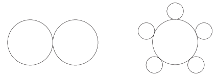
Figure 2: Diagrams contributing to the pressure at order $g^{2}$ (left diagram) and $g^{3}$ (right diagram).

II.2 Remarks about the coupling

The running of the coupling, to order one-loop, is governed by the $\beta$-function (5). Assuming an ultraviolet cut-off $\Lambda$, where the value of the coupling is $g_{\Lambda}$ and integrating Eq. (5), one gets:

$$\frac{1}{g_{\mu}^{2}}=\frac{1}{g_{\Lambda}^{2}}+\frac{9}{2\pi^{2}}\log\frac{\Lambda}{\mu},$$ (9)

which shows that $g_{\mu}\to 0$ when $\mu\to 0$. The coupling at scale $\mu=0$ is therefore not a suitable quantity to characterize the theory. In the following, we therefore adopt the usual practice of fixing the coupling at the scale $2\pi T$, which we shall simply denote by $g\equiv g(\mu=2\pi T)$ (unless ambiguities may arise). Equation (9) can then be rewritten as

$$\frac{1}{g_{\mu}^{2}}=\frac{1}{g^{2}}+\frac{9}{2\pi^{2}}\log\frac{2\pi T}{\mu}\,.$$ (10)

Now, for any finite value of $g$ there is a scale $\mu=\Lambda_{{\rm L}}$ (the “Landau pole”) at which the coupling diverges:

$$\Lambda_{{\rm L}}=2\pi T\exp\frac{2\pi^{2}}{9g^{2}}\,.$$ (11)

If $g\ll 1$ then $\Lambda_{\rm L}\gg\Lambda$ and the physics is not affected by $\Lambda_{\rm L}$. However, as $g$ grows, $\Lambda_{\rm L}$ decreases and eventually becomes of same order as $\Lambda$. In order to avoid unphysical behaviors, we require $\Lambda_{\rm L}>\Lambda$, which puts a constraint on the largest admissible values of $g$:

$$g^{2}<\frac{2\pi^{2}}{9\log(\Lambda/2\pi T)}\,.$$ (12)

It is easy to verify that this bound corresponds to an infinite value of $g_{\Lambda}$. To increase the maximum value of $g$, one could increase the temperature; however if $2\pi T$ becomes too close to $\Lambda$, the results become sensitive to the value of the cut-off (see the section on numerical results for further discussion of this point). Note that this estimate of the upper bound for $g$ is modified by non-perturbative effects, as we shall see in Sec. IV.

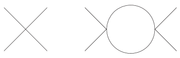
Figure 3: Diagrams contributing to the four-point function at order $g^{2}$ (left diagram) and $g^{4}$ (right diagram).

The coupling constant may be viewed as the value of the scattering amplitude $A$ for vanishing external momenta. While, as we have just seen, after renormalization this scattering amplitude vanishes, this is not so at finite temperature. Up to order $g^{4}$, $A$ can be calculated from the diagrams in Fig. 3. We obtain

$$A=g^{2}+36g^{4}T\sum_{\omega_{n}}\int\frac{d^{3}q}{(2\pi)^{3}}\left(\frac{1}{\omega_{n}^{2}+q^{2}+m_{D}^{2}}\right)^{2}.$$ (13)

We can calculate the sum-integral using the formulae given in Appendix A or, more directly, noticing that the thermal contribution is infrared dominated, by keeping only the contribution of $\omega_{n}=0$ in (13). We obtain

$$A \approx g^{2}-\frac{18g^{4}}{\pi^{2}}\int_{0}^{\infty}q^{{}^{2}}dq\frac{T}{\omega_{q}^{4}}=g^{2}-\frac{9g^{3}}{2\pi},$$ (14)

where $g^{2}=g^{2}(2\pi T)$. Thus the scattering amplitude contains a $g^{3}$ contribution, whose origin is the same as that of the $g^{3}$ contributions in the mass or the pressure.

II.3 Self-consistent 2PI resummation

As we have seen earlier, resummations are required in order to deal with the IR aspects of thermal perturbation theory. We shall briefly recall here the equations that are obtained in the simple $\Phi$–derivable approximation where the single 2PI diagram that is considered is the left diagram in Fig. 2. It is easily verified that this approximation is exact in the large $N$ limit, in the sense that it realizes the resummation of all the diagrams that survive this limit.

With this method, one obtains the following renormalized self-consistent gap equation for the mass $m$

$$m^{2}\,=\,12g_{\mu}^{2}\int\frac{{\rm d}^{3}k}{(2\pi)^{3}}\,\frac{n(\varepsilon_{k})}{\varepsilon_{k}}\,+\,\frac{3g_{\mu}^{2}m^{2}}{4\pi^{2}}\left(\log\frac{m^{2}}{\bar{\mu}^{2}}\,-1\right).$$ (15)

where the renormalized coupling $g_{\mu}$ is related to the bare one $g_{B}$ by ($\epsilon=4-d$):

$$\frac{1}{g^{2}_{\mu}}=\frac{\mu^{\epsilon}}{g_{B}^{2}}+\frac{3}{2\pi^{2}\epsilon}.$$ (16)

By using Eq. (16), one can check that the solution $m^{2}$ of Eq. (15) is independent of $\mu$ (to all orders in $g$). It is easily seen that the $\beta$-function that is deduced from Eq. (16) is only one third of the one-loop $\beta$-function (see Eq. (5)). This is a peculiar feature of $\Phi$-derivable approximations Blaizot et al. (2004): the particular resummation involved in the solution of the gap equation corresponds, for the scattering amplitude, to the iteration of the basic vertex in a single channel out of three. The correct one-loop $\beta$-function is recovered when one keeps in the $\Phi$-derivable approximation the skeleton of order $g^{4}$ Blaizot et al. (2004).

One can also easily compute the pressure

$$P=-T\int\frac{{\rm d}^{3}k}{(2\pi)^{3}}\,\log(1-{\rm e}^{-\beta\varepsilon_{k}})+\frac{m^{2}}{2}\int\!\!\frac{d^{3}k}{(2\pi)^{3}}\,\frac{n(\varepsilon_{k})}{2\varepsilon_{k}}\,+\frac{m^{4}}{128\pi^{2}}\,.$$ (17)

One can verify explicitly, but this is obvious from a simple analysis of the diagrammatic content of the approximation, that this expression for the pressure is perturbatively correct to order $g^{3}$. Besides, the complete, self-consistent results, as obtained by numerical evaluation of Eqs. (15) and (17), extrapolate smoothly to large values of $g$. We present the numerical results of the self-consistent mass and pressure in Sec. IV (in Figs. 13 and 15) when we compare them to the results obtained in this paper by RG techniques.

III Non-perturbative renormalization group

The basic strategy of the NPRG Ringwald and Wetterich (1990); Berges et al. (2002); Bervillier (2005) consists in adding to the classical action (2) a regulator, conveniently defined in momentum space as

$$\Delta S_{\kappa}[\varphi]=\frac{T}{2}\sum_{\omega_{n}}\int\frac{d^{d-1}q}{(2\pi)^{d-1}}\varphi_{i}(q)R_{\kappa}(q)\varphi_{i}(-q),$$ (18)

where $q=(q_{0}=i\omega_{n},{\bf q})$, with the Matsubara frequencies $\omega_{n}=2\pi nT$ and $R_{\kappa}$ is a cutoff function, depending on the continuous parameter $\kappa$, whose specific form will be given shortly. The role of $\Delta S_{\kappa}$ is to suppress the fluctuations with momenta $q\lesssim\kappa$, while leaving unaffected those with $q\gtrsim\kappa$. Thus typically $R_{\kappa}(q)\rightarrow\kappa^{2}$ when $q\ll\kappa$ and $R_{\kappa}(q)\rightarrow 0$ when $q\gg\kappa$. There is a large freedom in the choice of $R_{\kappa}(q)$, abundantly discussed in the literature Ball et al. (1995); Comellas (1998); Liao et al. (2000); Litim (2000, 2001a); Polchinski (1984); Litim (2001b); Canet et al. (2003a).

In this paper, we use a regulator which depends only on the spatial components of the momenta, ${\bf q}$, but not on the energy variable $q_{0}$. It is chosen of the form

$$R_{\kappa}^{{\rm th}}({\bf q}) = (\kappa^{2}-{\bf q}^{2})\theta(\kappa^{2}-{\bf q}^{2}).$$ (19)

A regulator that preserves Euclidean invariance, and is of the form of Eq. (19) with ${\bf q}\longrightarrow q$, could of course be used Litim (2000). However, such a regulator leads to several difficulties: since the regulator cuts off frequencies sharply, the contribution of single Matsubara frequencies become visible as we vary $\kappa$, resulting in an oscillatory behavior of the flows of various quantities. Furthermore, because the fluctuations are not entirely suppressed at the microscopic scale $\Lambda$ by such a regulator, initial conditions for quantities like the pressure need to be fine-tuned with temperature dependent counterterms. Although this can be done, it leads to unnecessary complications.

The NPRG constructs a family of effective actions $\Gamma_{\kappa}[\phi]$ (with $\phi$ the expectation value of the field), in which the magnitude of long wavelength fluctuations are controlled by the regulator $R_{\kappa}$. The effective action $\Gamma_{\kappa}[\phi]$ interpolates between the classical action obtained for $\kappa=\Lambda$ (with $\Lambda$ the microscopic scale at which the fluctuations are essentially suppressed) and the full effective action obtained when all fluctuations are taken into account, that is, when $\kappa\rightarrow 0$. One can write for $\Gamma_{\kappa}[\phi]$ an exact flow equation Tetradis and Wetterich (1994); Morris (1994a, b)

$$\partial_{\kappa}\Gamma_{\kappa}[\phi]=\frac{T}{2}{\rm tr}\sum_{\omega_{n}}\int\frac{d^{d-1}{\bf q}}{(2\pi)^{d-1}}\partial_{\kappa}R_{\kappa}({\bf q})\left[\Gamma_{\kappa}^{(2)}+R_{\kappa}\right]_{q,-q}^{-1}\,,$$ (20)

where $\Gamma^{(2)}_{\kappa}$ is the second derivative of $\Gamma_{\kappa}$ with respect to $\phi$.

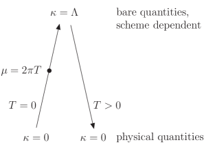
Figure 4: Basic concept of how to apply the flow equation at finite temperature. The coupling $g$ is extracted from the vacuum flow at the scale $\kappa=\mu$ with $\mu=2\pi T$.

Conceptually, we will follow the strategy developed in Ref. Tetradis and Wetterich (1993) and apply the flow equations in the way illustrated in Fig. 4: Starting with given physical parameters at $\kappa=0$, we integrate the flow equations up from $\kappa=0$ to $\Lambda$ thereby removing quantum fluctuations step by step in order to arrive at bare quantities at a chosen scale $\Lambda$. If $\Lambda$ is chosen big enough, only renormalizable parameters survive and the system can be described by a simple set of bare parameters. Starting from these bare parameters we can follow the flow down from $\kappa=\Lambda$ to 0, but this time with the temperature $T$ turned on. The physical quantities are then obtained at $\kappa=0$.

Note however that the coupling constant is fixed at the scale $\kappa=2\pi T$ on the $T=0$ flow, as discussed above. As for the mass at scale $\Lambda$, it is adjusted so that the mass at $\kappa=0$ vanishes. Note that this procedure induces a specific scheme dependence attached to the choice of the regulator. We should keep in mind this scheme dependence when comparing with results of perturbation theory or those of the 2PI resummation, that are obtained in another scheme.

Computationally, it might be numerically hard to integrate the flow equations up from $\kappa=0$ to $\Lambda$. But this is just equivalent to integrating them down, while carefully adjusting the bare parameters such that the flow will arrive at physically desired quantities at the end of the flow at $\kappa=0$.

III.1 Local potential approximation

A commonly used approximation to solve the flow equation for $\Gamma_{\kappa}[\phi]$ at zero external momenta is the local potential approximation (LPA). In this approximation, one assumes that the effective action has the form Morris (1994c); Berges et al. (2002)

$$\Gamma_{\kappa}^{{\rm LPA}}[\phi]=\int_{0}^{\beta}d\tau\int d^{d-1}x\left\{\frac{1}{2}\partial_{\mu}\phi_{i}\partial_{\mu}\phi_{i}+V_{\kappa}(\rho)\right\},$$ (21)

where $\rho\equiv\phi_{i}\phi_{i}/2$ and $V_{\kappa}(\rho)$ is the effective potential. The propagator of the scalar field can be decomposed into its transverse ($G_{T}$) and longitudinal ($G_{L}$) components:

$$G_{ij}(\kappa;q)=G_{T}(\kappa;q)\left(\delta_{ij}-\frac{\phi_{i}\phi_{j}}{2\rho}\right)+G_{L}(\kappa;q)\frac{\phi_{i}\phi_{j}}{2\rho}\,.$$ (22)

The equation for the potential, derived from Eq. (20) by assuming $\phi$ to be constant, then reads

$$\partial_{\kappa}V_{\kappa}(\rho)=\frac{T}{2}\sum_{\omega_{n}}\int\frac{d^{d-1}{\bf q}}{(2\pi)^{d-1}}\left[\partial_{\kappa}R_{\kappa}({\bf q})\right]\left\{\left(N-1\right)G_{T}(\kappa;q)+G_{L}(\kappa;q)\right\},$$ (23)

with

$$G_{T}(\kappa;q) = \frac{1}{q^{2}+V^{\prime}_{\kappa}(\rho)+R_{\kappa}(q)}\,,$$ (24)

$$G_{L}(\kappa;q) = \frac{1}{q^{2}+V^{\prime}_{\kappa}(\rho)+2\rho V^{\prime\prime}_{\kappa}(\rho)+R_{\kappa}(q)}\,,$$ (25)

with $V^{\prime}_{\kappa}(\rho)=dV_{\kappa}/d\rho$ and $V^{\prime\prime}_{\kappa}(\rho)=d^{2}V_{\kappa}/d\rho^{2}$. The LPA may be viewed as the leading order in a systematic expansion of the effective action in powers of the derivatives of the field. Such an expansion has been shown to exhibit quick apparent convergence if the regulator is appropriately chosen Litim (2001a); Canet et al. (2003a, b); Bagnuls and Bervillier (2001).

The choice (19) of the regulator leads to the following flow equation for the potential (see App. A)

$$\partial_{\kappa}V_{\kappa}(\rho) = K_{d-1}\kappa^{d}\left\{\left(N-1\right)\frac{2n(\omega_{\kappa}^{T})+1}{2\omega_{\kappa}^{T}}+\frac{2n(\omega_{\kappa}^{L})+1}{2\omega_{\kappa}^{L}}\right\},$$ (26)

where we have defined

$$\omega_{\kappa}^{T} \equiv \sqrt{V^{\prime}_{\kappa}(\rho)+\kappa^{2}},$$

$$\omega_{\kappa}^{L} \equiv \sqrt{V^{\prime}_{\kappa}(\rho)+2\rho V^{\prime\prime}_{\kappa}(\rho)+\kappa^{2}}\,.$$ (27)

Here, $n(q_{0})=(\exp(q_{0}/T)-1)^{-1}$ is the bosonic distribution function and $K_{d}=S_{d}/(d(2\pi)^{d})$ with $S_{d}=2\pi^{d/2}/\Gamma(d/2)$. In the cases that we shall study below, either the second ($N=1$ scalar theory) or the first term (large $N$ limit) in the braces will contribute to the flow. Note that, because of the one-loop structure of the flow equation, the r.h.s. of Eq. (26) naturally separates into a “thermal contribution”, which involves the statistical factors and which vanishes when $T\rightarrow 0$, and a “vacuum contribution” that contains no statistical factors.

III.2 Truncation and elementary analysis of the flow equations

In the next section, we shall present numerical solutions of the flow equation, Eq. (26). However, much insight can be gained by considering a simplified version of this equation, obtained by expanding the potential $V(\rho)$ around $\rho=0$ so that $m_{\kappa}^{2}=V_{\kappa}^{\prime}(\rho)|_{\rho=0}$ and $g_{\kappa}^{2}=V_{\kappa}^{\prime\prime}(\rho)|_{\rho=0}/8$. We shall give only the formulae for the case $N=1$, but they easily generalize to arbitrary $N$. We start from the flow equation (26) and insert a truncated potential of the form

$$V_{\kappa}(\phi) = V_{\kappa}+\frac{m_{\kappa}^{2}}{2}\phi^{2}+g_{\kappa}^{2}\phi^{4}+h_{\kappa}^{2}\phi^{6}+\dots$$ (28)

$$= V_{\kappa}+m_{\kappa}^{2}\rho+4g_{\kappa}^{2}\rho^{2}+8h_{\kappa}^{2}\rho^{3}+\dots$$

Truncating the series at order $O(\rho^{3})$, and neglecting $h_{\kappa}$ and higher order coefficients, result in replacing $V^{\prime}_{\kappa}(\rho)+2\rho V^{\prime\prime}_{\kappa}(\rho)+\kappa^{2}$ by $\kappa^{2}+m_{\kappa}^{2}+24g_{\kappa}^{2}\rho$. We obtain the following set of coupled differential equations at orders $\rho^{0}$, $\rho$, and $\rho^{2}$:

$$O(\rho^{0}):\quad\partial_{\kappa}V_{\kappa} = K_{d-1}\kappa^{d}\frac{1+2n\left(\epsilon_{\kappa}\right)}{2\epsilon_{\kappa}}\,,$$ (29)

$$O(\rho^{1}):\quad\partial_{\kappa}m_{\kappa}^{2} = -6g_{\kappa}^{2}K_{d-1}\kappa^{d}\frac{1+2n\left(\epsilon_{\kappa}\right)-2\epsilon_{\kappa}n^{\prime}(\epsilon_{\kappa})}{\epsilon_{\kappa}^{3}}\,,$$ (30)

$$O(\rho^{2}):\quad\partial_{\kappa}g_{\kappa}^{2} = 27g_{\kappa}^{4}K_{d-1}\kappa^{d}\frac{1+2n\left(\epsilon_{\kappa}\right)-2\epsilon_{\kappa}n^{\prime}(\epsilon_{\kappa})+\frac{2}{3}\epsilon_{\kappa}^{2}n^{\prime\prime}(\epsilon_{\kappa})}{\epsilon_{\kappa}^{5}}\,$$ (31)

with the short-hand notation $\epsilon_{\kappa}:=\sqrt{\kappa^{2}+m_{\kappa}^{2}}$. The right hand side of Eq. (31) would change if one wanted to include the coupling $h_{\kappa}$ (of order $g_{\kappa}^{6}$), but Eqs. (29) and (30) would not. These equations have a simple interpretation in terms of the diagrams depicted in Figs. 5, 6, and 7: these diagrams can be easily calculated with the formulae given in Appendix A for the finite temperature loop integrals.

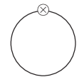
Figure 5: Diagrammatic illustration of the r.h.s. of the flow equation of the effective action, Eq. (29). The crossed circle represents an insertion of the regulator $\partial_{\kappa}R_{\kappa}$, and the thick line a full propagator with mass $m_{\kappa}$.

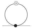
Figure 6: Diagrammatic illustration of the r.h.s. of the flow equation for the 2-point function, e.g. the mass, Eq. (30). The black dot denotes the four-point function (the coupling $g_{\kappa}$) and the thick line the full propagator $G_{\kappa}$ (including the regulator, see Eqs. (24), (25)). The circled cross represents the insertion of $\partial_{\kappa}R_{\kappa}$.

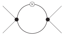
Figure 7: Diagrammatic illustration of the r.h.s. of the flow equation for the 4-point function, showing the contribution to the flow of the coupling $g_{\kappa}$ included in Eq. (31) (the contribution of the 6–point function is ignored in this equation). Black disks represent the coupling $g_{\kappa}$. The three channels are included in (31) by the proper factor 3 (external momenta vanish). The crossed circle represents an insertion of $\partial_{\kappa}R_{\kappa}$, and the thick line a full propagator.

The general character of the flow can easily be inferred from a simple analysis of Eqs. (29), (30) and (31). For instance, the coupling follows a four-dimensional flow from $\Lambda$ to $\kappa\approx 2\pi T$, then a three dimensional flow before it freezes when $\kappa\simeq m_{D}$. This can be seen from Eq. (31): At large values of $\kappa$, the bosonic distribution function can be neglected and $\epsilon_{\kappa}\approx\kappa$ so that $\partial_{\kappa}g_{\kappa}^{2}\propto g_{\kappa}^{4}/\kappa$ and we recover the characteristic logarithmic flow in $d=4$ dimensions. In the opposite limit $\kappa\rightarrow 0$, the value of $\epsilon_{\kappa}$ is limited by the thermal mass $\epsilon_{\kappa}\approx m_{D}\sim gT$ (see Eq. (7)), and the flow becomes $\partial_{\kappa}g_{\kappa}^{2}\propto g_{\kappa}^{4}\kappa^{4}$, leading quickly to a constant value for $g_{\kappa}^{2}$. In the intermediate range when we still have $\kappa\gtrsim m_{\kappa}$ and thus $\epsilon_{\kappa}\approx\kappa$, but one can already expand the thermal distribution function for $\kappa\lesssim T$ (see Eq. (44) below), one finds $\partial_{\kappa}g_{\kappa}^{2}\propto g_{\kappa}^{4}/\kappa^{2}$, which is compatible with a three dimensional flow, with $g_{\kappa}\sim\kappa$ at small $\kappa$. This qualitative behavior will be confirmed by the numerical results presented in the next section.

IV Numerical results

The numerical integration of the flow equation (26) (using the Runge-Kutta method with adaptive step-size) is hampered by the flow of the potential over several orders of magnitude. In order to keep the zero-temperature flow under control, one can introduce dimension-less variables Berges et al. (2002), but these will not be suitable for the thermal flow, which freezes in dimensionful variables (but would diverge in dimensionless variables as $\kappa\rightarrow 0$). However, one can take advantage of the fact that a large part of the flow cancels between thermal and vacuum contributions, as will be described in subsection IV.3, and obtain useful results for the potential, and therefore the pressure, mass, and coupling. In the first part of this section, we present results for the scalar theory with $N=1$ component, and in the last subsection for the large $N$ limit where the LPA becomes exact D’Attanasio and Morris (1997); Tetradis and Litim (1996).

IV.1 Coupling

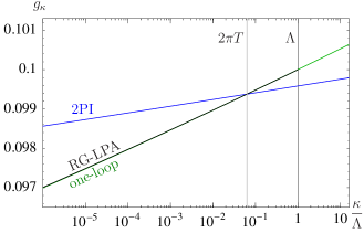
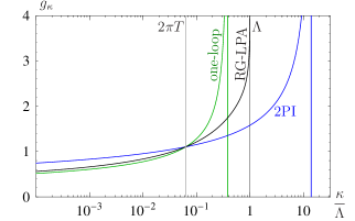
Figure 8: Comparison of the flow of the coupling at zero temperature for $g\equiv g(2\pi T)=0.0994$ ($g_{\Lambda}=0.1$) and for $g=1.1032$ ($g_{\Lambda}=4$). At weak coupling one observes that the 2PI $\beta$-function differs form the one-loop result by a factor $1/3$. At larger coupling the Landau pole is observed in the running of the coupling.

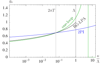
Figure 9: Same as Fig. 8 for $g=0.699$ ($g_{\Lambda}=1$).

Figures 8 and 9 show the LPA flow of the coupling $g_{\kappa}$ at zero temperature, for different values of the $g=g(2\pi T)$, comparing with one-loop results as well as with those of the self-consistent approximation described in Sec. II. The three plots correspond to $T=\Lambda/100$, and the numerical correspondence between $g$ and bare coupling $g_{\Lambda}$ is indicated in the caption. By construction, the curves cross each other at the scale $\kappa=2\pi T$. As shown by the left panel of Fig. 8 the LPA $\beta$-function agrees with the one-loop $\beta$-function, Eq. (5), at weak coupling, reflecting the scheme independence of its first coefficients. Also visible on Fig. 8 is the fact, already mentioned, that the 2PI resummation scheme leads to a $\beta$-function that is smaller by a factor $3$. As discussed in section II.2, at larger couplings (right panel of Fig. 8), all three curves exhibits the presence of the Landau pole where $g_{\kappa}$ diverges. Note that the perturbative estimate of the position of the Landau pole in Eq. (11) is exceeded by the NPRG flow, and the moderate 2PI flow predicts a Landau pole that lies further away. The one-loop calculation in Fig. 8 (right panel) does not make sense for the large value of the coupling since then, as seen in the right panel of Fig. 8, $\Lambda_{\rm L}<\Lambda$. Figure 9 shows the flow at some intermediate coupling $g(2\pi T)=0.699$ ($g_{\Lambda}=1$).

Thus, the presence of the Landau pole limits the applicability of the NPRG to not too large couplings, as already discussed in Sec. II.2. There is however another limitation that comes from the fact that the denominator in (26), given by (27), becomes imaginary. This is to be expected to happen when the coupling gets too large, as can be seen from the perturbative estimate: $V_{\Lambda}^{\prime}(0)=m_{\Lambda}^{2}\approx-g_{\Lambda}^{2}\Lambda^{2}/(2\pi^{2})$ (see Eq. (40) below).

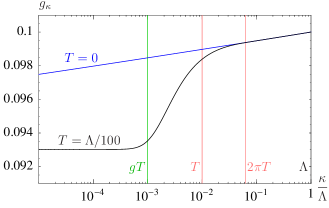
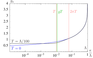
Figure 10: Flow of the coupling at finite temperature for $g=0.0994$ ($g_{\Lambda}=0.1$), left, and for $g=1.1032$ ($g_{\Lambda}=4$), right. For the smaller coupling, the value of $g_{\kappa}$ drops only moderately from $\kappa=\Lambda$ to $2\pi T$ and the thermal coupling reaches a fixed value at $g_{\kappa=0}=0.093$. For the larger coupling, the beta function forces a steep drop from $g_{\Lambda}=4$ to $g=1.1032$, and further to $g_{\kappa=0}=0.68$ for the thermal coupling.

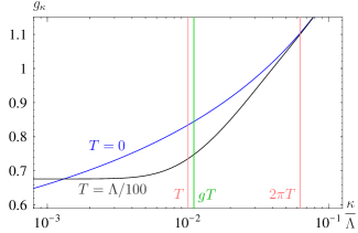
Figure 11: Enlarged view of Fig. 10 (right) to show the region of dimensionally reduced flow.

In Fig. 10 we turn on the temperature, and compare the vacuum flow with the flow obtained at a temperature $T=\Lambda/100$. At weak coupling (left panel of Fig. 10), the scales $gT$ and $T$ are well separated, and we observe the general features discussed in Sec. III.2: From $\kappa=\Lambda$ down to $2\pi T$, the vacuum ($T=0$) flow of the coupling and the thermal flow agree. While the vacuum flow continues to decrease logarithmically all the way down to $\kappa=0$, below $\kappa=2\pi T$ the thermal flow starts to deviate from the vacuum flow in a dimensionally reduced manner. The three-dimensional flow stops at the scale $\kappa\sim gT$, where the thermal mass is generated. The situation does not change qualitatively for larger values of the coupling in the right panel of Fig. 10 (enlarged in Fig. 11): The main difference is that the range of the three-dimensional flow shrinks as $gT$ approaches $T$. We shall return to this at the end of the next subsection.

IV.2 Mass

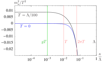
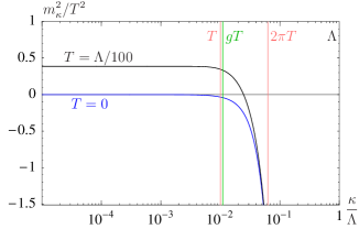
Figure 12: Flow of the mass for $g=0.0994$ ($g_{\Lambda}=0.1$), left, and for $g=1.1032$ ($g_{\Lambda}=4$), right. The mass reaches the value $m=0.094T$ for $g=0.0994$ and $m=0.622T$ for $g=1.1032$ as $\kappa\rightarrow 0$. (For $T=0$, the quantity plotted is $m_{{\rm vac},\kappa}^{2}/T^{2}$.)

The freezing of the flow at soft scales is caused by the thermally generated mass $m_{\kappa}^{2}=V^{\prime}_{\kappa}(\rho=0)$, shown in Fig. 12. As is the case for the coupling, the flow in the range $2\pi T\lesssim\kappa\leq\Lambda$ agrees between vacuum and thermal flow. The system starts at a large negative mass squared, which can be estimated perturbatively as $m_{\Lambda}^{2}=-g_{\Lambda}^{2}\Lambda^{2}/(2\pi^{2})+O(g_{\Lambda}^{4})$, see Eq. (40). In the course of the flow, the mass acquires positive contributions through quantum fluctuations. The initial condition $m_{\Lambda}^{2}$ has been tuned at zero temperature, such that $m_{\kappa=0}^{2}$ vanishes. At finite temperature, the flow of the mass deviates below the scale $\kappa=2\pi T$ and builds up the thermal mass $m\simeq gT$ that can be observed in Fig. 12.

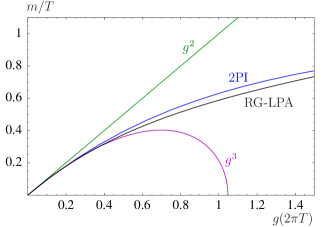
Figure 13: Thermal mass for scalar theory with $N=1$ component as a function of the coupling. The result obtained from the non-perturbative renormalization group labeled “RG-LPA” gets close to the result obtained by 2PI resummation. Both show moderate behavior where the perturbative contributions represented by curves of order $g^{2}$ and $g^{3}$ fail to converge.

The values obtained from the flow equation in Figs. 10 and 12 are combined to produce the result displayed in Fig. 13. For example, starting the numerical calculation from $g_{\Lambda}=4$, one obtains a coupling $g=g(2\pi T)=1.1032$. At this value of the coupling, the mass takes the value $m/T=0.622$ (Fig. 12) in the physical limit $\kappa\rightarrow 0$. This information is put into Fig. 13, and the procedure is repeated for other values of the coupling. The curve thus obtained, labeled “RG-LPA”, is smooth, in contrast to those displaying the results of strict perturbation theory through orders $g^{2}$ and $g^{3}$. For comparison, in Fig. 13 we also plot the results obtained through the 2PI resummation described in Sec. II Blaizot et al. (2001). The difference obtained between the RG-LPA and 2PI approaches has two origins: on the one hand, the two calculations correspond to two different $\beta$-functions: $\beta_{\rm 2PI}=\beta_{\rm one-loop}/3$ (see Fig. 8). On the other hand, the two calculations use different renormalization schemes: the 2PI curve shows the scale choice in the $\overline{{\rm MS}}$-scheme with $\bar{\mu}_{\overline{{\rm MS}}}=2\pi T$. In comparison, the NPRG approach defines the coupling from the vacuum flow at $\kappa=2\pi T$ and the quantities at other scales depend on the choice of the regulator.

From Figs. 10 to 13 we can already extract one of the main results of our work. Both in the weak and the strong coupling regimes, the scale dependence of the running coupling and of the mass exhibits a similar behavior: in both cases, thermal effects start to play a role around $\kappa\simeq 2\pi T$ and saturate at $\kappa\simeq m_{D}\simeq gT$. When going from weak to strong coupling, there is a competition between two effects: on the one side, the range of the values of $\kappa$ where thermal effects are important shrinks because the thermal mass increases with the coupling; on the other side, the amplitude of the three-dimensional flow increases with increasing values of $g$. Both effects are visible in Figs. 10 and 11. The net effect is that the variation of the coupling along the three dimensional flow is limited; for instance, in Fig. 11 for $g=1.1032$, it amounts to a 30% effect.

One can also observe in Fig. 11 that, at strong coupling, the flow saturates at a value of $\kappa\lesssim gT$. This is because the thermal mass reaches a value lower than $gT$, as illustrated in Fig. 13. In fact, one may argue that the thermal mass cannot exceed a value $\simeq 2\pi T$, since otherwise all thermal effects would disappear, which is in contradiction with the existence of such thermal mass.

IV.3 Pressure

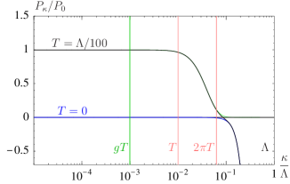
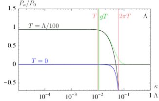
Figure 14: Comparison of the flow of the pressure in the weak-coupling regime for $g=0.0994$ ($g_{\Lambda}=0.1$), left panel, and in the strong-coupling regime for $g=1.1032$ ($g_{\Lambda}=4$), right panel, with $T=\Lambda/100$. The additive constant is chosen such that the vacuum pressure vanishes as $\kappa\rightarrow 0$. The thermal pressure reaches the value of $P=0.9984P_{0}$ for $g=0.0994$ and $P=0.945P_{0}$ for $g=1.1032$ as $\kappa\rightarrow 0$.

Figure 14 shows the flow of the pressure $P=-V(\rho=0)$ for weak and strong couplings, normalized to the free pressure $P_{0}=(\pi^{2}/90)T^{4}$. We choose $V_{\Lambda}(\rho=0)$ such that the zero-temperature pressure $P_{\kappa=0}(T=0)$ vanishes. This requires however a delicate cancellation. Indeed, a perturbative calculation (see Eq. (39) below) shows that the vacuum pressure at $\kappa=\Lambda$ is of the order $\Lambda^{4}$. Thus, for example, both curves for the $g=1.1032$ plot start at $P_{\Lambda}=-415,470.518P_{0}$ and acquire a relative difference during the flow from $\kappa=\Lambda$ to $\kappa=0$ of $0.945P_{0}$. Clearly, this cancellation over six orders of magnitude poses a challenge to the numerics. One should note though that the thermal flow above $\kappa\gtrsim 2\pi T$ lies exponentially close to the zero temperature flow due to the bosonic distribution function in Eq. (26), and the bulk of the thermal contribution builds up between $\kappa\simeq 2\pi T$ and $\kappa\simeq gT$. This difference between thermal and vacuum flows is shown as a light curve in the plots. It is therefore sufficient to start the integration of the thermal pressure at some intermediate scale $2\pi T\ll\Lambda_{1}\ll\Lambda$. The zero-temperature and finite-temperature flows of the potential only reach a maximum value of the order of $\Lambda_{1}^{4}\lll\Lambda^{4}$ and their difference is numerically much easier to handle. On the other hand, $\Lambda_{1}$ can not be chosen too small, or contributions to the result will be neglected. Practically, a value of $\Lambda_{1}=20T$ turned out to be a good compromise between loss of accuracy due to neglecting $\kappa\geq\Lambda_{1}$ contributions and gain of accuracy due to reduced numerical cancellation. This procedure also improves the numerical accuracy of the thermal mass, shown in Fig. 12, although the situation is not as critical there (the mass only grows as $\kappa^{2}$, as opposed to the pressure that grows as $\kappa^{4}$).

Since the pressure, mass, and coupling constant all approach constant values as $\kappa\to 0$, dimensionless variables that one may introduce for the zero-temperature flow cease to be useful: For example, as the dimensionful potential $V_{\kappa\rightarrow 0}$ approaches a constant, the dimensionless variable diverges as $v_{\kappa\rightarrow 0}\sim 1/\kappa^{d}$. Numerically, we have still followed the approach of dimensionless variables also for thermal quantities, as $\kappa$ does not need to become too small to measure the limiting value reached when $\kappa\rightarrow 0$.

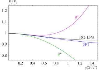
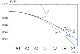
Figure 15: Pressure as a function of the coupling (left panel) and as a function of the mass (right panel). As two physical, scale-independent quantities are compared, the right plot is renormalization scale independent and shows an improved agreement between RG-LPA and 2PI results.

The left panel of Fig. 15 shows the pressure as a function of $g$. It follows combining results from Figs. 10 and 14, in the same way as Figs. 10 and 12 lead to Fig. 13. Due to the limitations of the maximum value of the coupling that we can use (see discussion on page IV.1), it is necessary to reduce the ratio $T/\Lambda$ for the larger couplings in Fig. 15. The range depicted (up to $g\approx 1.5$) is about the range in which both pressure and thermal mass are still independent of this choice of $T/\Lambda$, up to plot accuracy. For the largest $g\sim 1.5$ we have chosen $T/\Lambda=1/20$; this agrees for smaller $g$ with $T/\Lambda=1/50$ or $1/100$. The value $T/\Lambda=1/10$ could extend the NPRG method to even larger $g$, but then the result visibly starts to deviate from the $T/\Lambda=1/20$ result. Similar to the plot for the mass in Fig. 13, we observe an improved result “RG-LPA” over perturbation theory through orders $g^{2}$ and $g^{3}$. We obtain a deviation of similar magnitude when compared to the 2PI resummation scheme, part of which is caused as mentioned above by different renormalization schemes. Note that the 2PI curve lies below the RG-LPA curve.

We can circumvent the problem of renormalization scale by comparing only physical quantities. Figure 15 (right panel) displays the pressure as a function of the mass. For the LPA curve, both quantities, pressure and mass, are extracted at $\kappa=0$, so there is no more reference in this plot to a particular choice of a scale for the coupling $g$. The perturbative contributions $g^{2}$ and $g^{3}$ on the other hand can be considered as scale-independent only up to the order they have been calculated to. These curves may change when extracted at a different scale. In this plot we observe improved agreement between the RG-LPA curve and the 2PI curve, but also note that they do not completely agree. Particularly, at larger $m/T$, the LPA curve starts to bend up again. This is the region where the NPRG equations get sensitive to the Landau pole and may also fail because of imaginary parts in the denominator of the flow equation as discussed on page IV.1, so this region should be considered with care (the fact that the 2PI curve does not show the same bending as the RG-LPA one presumably reflects the fact that the 2PI Landau pole is artificially pushed to higher values because of the factor $1/3$ in the 2PI $\beta$-function). The break-down of perturbation theory can be pinpointed where the $g^{3}$ contribution deviates visibly. This curve bends backwards, because $m(g)$ is not a monotonous function at this order. Surprisingly, the $g^{2}$ curve seems to remain a good approximation to the non-perturbative approaches.

IV.4 Large $N$ limit

In the large $N$ limit, only the transverse propagator in Eq. (26) contributes to the flow. The various quantities scale in the following way as $N\rightarrow\infty$:

$$P,\,V,\,\rho \sim N\,,$$

$$V^{\prime}_{\kappa}(\rho),\,m^{2} \sim 1\,,$$

$$g^{2} \sim 1/N\,.$$ (32)

It is then advantageous to plot results as a function of an effective coupling $g_{{\rm eff}}\equiv g\sqrt{N}$. Note that both $P/P_{0}$ and $m/T$ are $N$-independent quantities.

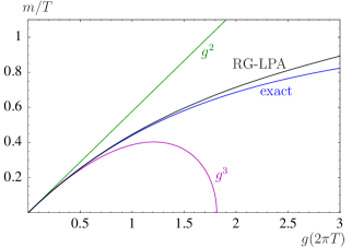
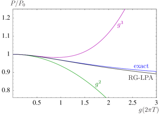
Figure 16: Comparison of mass (left panel) and pressure (right panel) at large $N$, normalized to temperature and the free pressure, respectively. The coupling $g$ denotes the effective coupling $g_{{\rm eff}}=g\sqrt{N}$ in the limit $N\rightarrow\infty$.

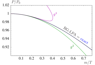
Figure 17: Pressure as a function of the mass in the large $N$ limit. In the comparison of scale-independent quantities, the RG-LPA numerical result exactly reproduces the large $N$ limit.

In Fig. 16 we plot the predictions of the RG-LPA for the mass and the pressure as a function of the coupling constant, together with the exact large $N$-limit results, which are known (see e.g. Blaizot et al. (2003a)). In the large $N$ limit, the LPA approximation also gets exact D’Attanasio and Morris (1997); Tetradis and Litim (1996). The reason why the curves of Fig. 16 do not exactly agree is because of the already mentioned scheme dependence. If one plots only scale-independent quantities, like the pressure as a function of the thermal mass, then one recovers indeed a full agreement between the RG-LPA and the known exact large $N$ limit results (see Fig. 17).

V Perturbative expansion of the flow equation

In the spirit of other resummation schemes proposed in the literature, we show that the NPRG in the LPA, reproduces perturbation theory up to order $g^{3}$. Of course, the full numerical evaluation of the flow equation in Sec. IV includes higher orders in a non-perturbative way.

We start from the truncated flow equations (29) to (31) where the neglected term in (28), $h_{\kappa}$, is of order $g_{\kappa}^{6}$. These equations for the mass (30) and coupling constant (31) from a closed set of equations that can be solved order by order in $g$. The pressure can then be calculated using the results for $m_{\kappa}$ and $g_{\kappa}$.

In the case of the vacuum flow, the perturbative hierarchy is quite clear: $m_{\kappa}^{2}$ is always $\sim g_{\kappa}^{2}\kappa^{2}$, and one can therefore expand $\epsilon_{\kappa}=\sqrt{\kappa^{2}+m_{\kappa}^{2}}\simeq\kappa$ for all $\kappa$.

At finite temperature, on the other hand, a thermal mass of the order $gT$ is generated, and expanding for small $m_{\kappa}$ necessarily fails when $\kappa\lesssim gT$. In this case, it is useful to introduce an intermediate scale $\xi$ that lies between soft and hard momenta $gT\ll\xi\ll T$ (e.g. $\xi\sim\sqrt{g}\,T$). Different expansions can then be performed in these two regions: For hard momenta, $\kappa\gtrsim\xi$,

$$\epsilon_{\kappa}^{2}=\kappa^{2}+m_{\kappa}^{2}=\kappa^{2}\left(1+O((gT/\xi)^{2})\right).$$ (33)

For soft momenta, $\kappa\lesssim\xi$, we can expand the thermal distribution function

$$n(\kappa) = \frac{T}{\kappa}-\frac{1}{2}+\frac{\kappa}{12T}+\frac{T}{\kappa}O((\xi/T)^{3}).$$ (34)

The leading term, $T/\kappa$, trades one dimension of a $d$-dimensional integration by the temperature, thereby leading to a dimensionally reduced system. From the calculation of section II.1, one expects order $g^{2}$ contributions to arise from integrals dominated by hard momenta, and $g^{3}$ effects to build up at soft momenta. However, as we shall see, delicate cancellations occur in the course of the calculation. In order to cleanly reproduce strict perturbative results at order $g^{3}$, we shall expand the actual running quantities $g_{\kappa}$ or $m_{\kappa}$ around their leading order perturbative contributions:

$$g_{\kappa}^{2} = g^{2}+\delta g_{\kappa}^{2},$$

$$m_{\kappa}^{2} = m^{2}+\delta m_{\kappa}^{2},$$ (35)

with $m^{2}=g^{2}T^{2}$ (see (54)), where $g$ without subscript is to be understood, as before, as $g=g_{{\rm vac}}(\kappa=2\pi T)$. As we shall see, in the region $\kappa\geq\xi$ the correction $\delta g_{\kappa}^{2}$ will be formally of order $g^{4}$ (see (43)), while for $\kappa\leq\xi$ the correction $\delta g_{\kappa}^{2}$ will be formally of order $g^{3}$ (see (83)) and $\delta m_{\kappa}^{2}$ of the order $g^{2}\xi T$ (see (84) and (85)). Technical details that amount to $O(g^{4})$ or $O(g^{4}\ln g)$ contributions are deferred to App. B; the LPA is not expected to reproduce them correctly.

V.1 Zero-temperature flow

At zero temperature, all the distribution functions $n(\epsilon_{\kappa})$ and their derivatives vanish in Eqs. (29) to (31), and we are left with the following set of differential equations, that we expand in powers of $g_{\kappa}^{2}$,

$$\partial_{\kappa}V_{\kappa} = \frac{K_{d-1}\kappa^{d}}{2\epsilon_{\kappa}}\,=\,K_{d-1}\left(\frac{\kappa^{d-1}}{2}-\frac{m_{\kappa}^{2}\kappa^{d-3}}{4}\right)+O(g_{\kappa}^{4}),$$ (36)

$$\partial_{\kappa}m_{\kappa}^{2} = -\frac{6g_{\kappa}^{2}K_{d-1}\kappa^{d}}{\epsilon_{\kappa}^{3}}\,=\,-6g_{\kappa}^{2}K_{d-1}\kappa^{d-3}+O(g_{\kappa}^{4})\,,$$ (37)

$$\partial_{\kappa}g_{\kappa}^{2} = \frac{27g_{\kappa}^{4}K_{d-1}\kappa^{d}}{\epsilon_{\kappa}^{5}}\,=\,27g_{\kappa}^{4}K_{d-1}\kappa^{d-5}+O(g_{\kappa}^{6})\,.$$ (38)

In these equations, we anticipated that the mass $m_{\kappa}^{2}$ will be of order $g_{\kappa}^{2}$ (i.e. we assume that $m_{\kappa=0}$ vanishes, so that $m_{\kappa}^{2}$ is entirely due to quantum fluctuations). For $d=4$ the solutions of these equations read:

$$V_{\kappa} = V_{\Lambda}+\frac{\kappa^{4}-\Lambda^{4}}{48\pi^{2}}+O(g_{\Lambda}^{2}),$$ (39)

$$m_{\kappa}^{2} = -g_{\kappa}^{2}\frac{\kappa^{2}}{2\pi^{2}}+O(g_{\Lambda}^{4})\,,$$ (40)

$$g_{\kappa}^{2} = \frac{g_{\Lambda}^{2}}{1-9g_{\Lambda}^{2}\log(\kappa/\Lambda)/(2\pi^{2})}+O(g_{\Lambda}^{6})\,.$$ (41)

In deriving these equations, we have assumed that $g_{\Lambda}\ll 1$, and also taken into account the possible occurrence of large logarithms in getting Eq. (41). To get Eq. (40), one integrates the r.h.s. of Eq. (37) by parts using (38). Finally, the integration constant has been adjusted so that $m_{\kappa=0}^{2}$ vanishes, i.e. we have $m_{\Lambda}^{2}=-g_{\Lambda}^{2}\Lambda^{2}/(2\pi^{2})$. Using these results, we can actually proceed one order further in the potential:

$$V_{\kappa} = V_{\Lambda}+\frac{\kappa^{4}-\Lambda^{4}}{48\pi^{2}}+\frac{g_{\kappa}^{2}\kappa^{4}-g_{\Lambda}^{2}\Lambda^{4}}{192\pi^{4}}+O(g_{\Lambda}^{4}).$$ (42)

V.2 Coupling at finite temperature

In order to find the perturbative solution of Eq. (31) we introduce an intermediate scale $\xi$, as discussed above, with $gT\ll\xi\ll T$. For $\kappa\geq\xi$ thermal effects are subleading and $g_{\kappa}^{2}$ can be obtained directly from (41)

$$g_{\kappa}^{2}=g^{2}+\frac{9g^{4}}{2\pi^{2}}\log\frac{\kappa}{2\pi T}+O(g^{6}).$$ (43)

In the region $\kappa\leq\xi$ we can expand the distribution function in Eq. (31) according to (34) which gives a remarkably stable expansion (i.e. all powers from $\epsilon_{\kappa}^{0}$ to $\epsilon_{\kappa}^{4}$ drop out)

$$1+2n\left(\epsilon_{\kappa}\right)-2\epsilon_{\kappa}n^{\prime}(\epsilon_{\kappa})+\frac{2}{3}\epsilon_{\kappa}^{2}n^{\prime\prime}(\epsilon_{\kappa})=\frac{16T}{3\epsilon_{\kappa}}+\frac{\epsilon_{\kappa}^{5}}{5670T^{5}}+O(\frac{\epsilon_{\kappa}^{6}}{T^{6}})\,.$$ (44)

The flow equation then becomes

$$\partial_{\kappa}g_{\kappa}^{2}=\frac{24g_{\kappa}^{4}}{\pi^{2}}\frac{\kappa^{4}T}{\epsilon_{\kappa}^{6}}$$ (45)

with $\epsilon_{\kappa}^{2}=\kappa^{2}+m_{\kappa}^{2}$. By writing $m_{\kappa}^{2}=m^{2}+\delta m_{\kappa}^{2}$ (see Eq.  (35)), and expanding out the $\delta m_{\kappa}^{2}$ correction, we obtain for the leading contribution

$$\left.-\frac{1}{g_{\kappa}^{2}}\right|_{\kappa^{\prime}}^{\xi}=\left.\frac{3T}{\pi^{2}}\left(\frac{3}{m}\arctan\frac{\kappa}{m}-\frac{5\kappa^{3}+3\kappa m^{2}}{(\kappa^{2}+m^{2})^{2}}\right)\right|_{\kappa^{\prime}}^{\xi}+O(\xi/(gT)).$$ (46)

In the limit $\kappa^{\prime}\rightarrow 0$ and $gT\ll\xi\rightarrow\infty$ and expanding the result in $g$, we recover the result obtained earlier

$$g_{\kappa=0}^{2}=g^{2}-\frac{9}{2\pi}g^{3}+O(g^{3}\xi/T)\,.$$ (47)

(The expression for general $\kappa$ is given in (83)). Note that the result is, to order $g^{3}$, independent of the temperature $T$. This may seem at first sight surprising. However, the only possible effect of of the temperature is a change of the renormalization scale, and this only influences the result at order $O(g^{4})$. A careful calculation through order $g^{4}$ (presented in Appendix B.1) reveals how the value of the coupling at $\kappa=0$ is connected to the coupling at $\kappa\gtrsim T$:

$$g_{\kappa=0}^{2}=g_{\kappa}^{2}-\frac{9g_{\kappa}^{3}}{2\pi}-\frac{9g_{\kappa}^{4}}{2\pi^{2}}\left(\log\frac{\kappa}{2\pi T}+\gamma-\frac{61}{12}+\frac{32}{3{\pi}^{2}}\right)+O(g_{\kappa}^{5}),$$ (48)

where $\gamma$ is Euler’s constant. Note that this result is obtained from perturbatively expanding the flow equation within the LPA.

Figure 18: Same as Fig. 10, compared to analytic solutions. Dashed lines give perturbative solution through order $g^{3}$ (flowing with $\kappa$), with $g$ taken at $\kappa=2\pi T$, and $g^{4}$ (only $g_{0}$ value), with $g$ taken at $\kappa=2\pi T$. For the left panel, also the solution of truncated LPA is given by the light curve.

Figure 18 shows a comparison with the numerical solutions. The curves labeled “$g^{3}$” show the sum of the $g^{2}$ value at $\kappa=2\pi T$ and the $\kappa$-dependent correction of order $g^{3}$ from Eq. (83). This formula is strictly speaking only valid in a region $\kappa\leq\xi$ and introduces an error of the order ${\mathcal{O}}(gT/\xi)$. This error is the reason why the $g^{3}$ curve does not agree with the numerical value of $g$ at $\kappa=2\pi T$, but reaches this value only for $\kappa\rightarrow\infty$. Also, through order $g^{3}$ there is no renormalization scale dependence, and the analytical solution does not follow the vacuum flow of the numerical result. The curves labeled “$g^{4}$” in Fig. 18 show the result (48) with $g(\kappa=2\pi T)$.

For the left plot of Fig. 18 also the result of truncated LPA, obtained by numerically integrating Eqs. (29) to (31), is given. While for small coupling in the left plot of Fig. 18 the truncated LPA misses the full numerical result of the scattering amplitude $g_{\kappa=0}$ by 0.3%, at the larger coupling $g(\Lambda)=4$, the truncated LPA would underestimate the value of $g(\kappa=2\pi T)$ by 28% (not shown in the plot). If we instead lower the cutoff $\Lambda$ such that the vacuum couplings at $\kappa=2\pi T$ agree, the truncated LPA will give a result for $g_{\kappa=0}$ that is 23% larger than the full numerical result. Thus, while this truncation provides reliable estimates at small coupling, it cannot be used at strong coupling.

V.3 Thermal mass

We consider now finite temperature effects and focus first on the thermal mass. This is defined by separating the mass in equation (30) into vacuum and thermal pieces:

$$m_{{\rm vac},\kappa}^{2} = m_{\kappa}^{2}(T=0)\,,$$ (49)

$$m_{{\rm th},\kappa}^{2} = m_{\kappa}^{2}(T)-m_{{\rm vac},\kappa}^{2}\,.$$ (50)

The thermal contribution can then be calculated using $\epsilon_{\kappa}:=\sqrt{\kappa^{2}+m_{{\rm th},\kappa}^{2}+m_{{\rm vac},\kappa}^{2}}$, and reads:

$$m_{{\rm th},\kappa^{\prime}}^{2}=-6K_{d-1}\int_{\Lambda}^{\kappa^{\prime}}d\kappa\,\kappa^{d}\left\{g_{\kappa}^{2}\frac{1+2n(\epsilon_{\kappa})-2\epsilon_{\kappa}n^{\prime}(\epsilon_{\kappa})}{\epsilon_{\kappa}^{3}}-g_{{\rm vac},\kappa}^{2}\frac{1}{(\kappa^{2}+m_{{\rm vac},\kappa}^{2})^{3/2}}\right\}\,.$$ (51)

V.3.1 Thermal mass to leading order

As we have seen earlier, the $g^{2}$ contribution to the thermal mass is dominated by hard momenta. Using Eqs. (33) and (35), we obtain as leading contribution

$$m_{{\rm th},\kappa^{\prime}}^{2} = 12g^{2}K_{d-1}\int_{\kappa^{\prime}}^{\Lambda}d\kappa\,\kappa^{d-3}\left(n(\kappa)-\kappa n^{\prime}(\kappa)\right)+O(g^{4})\,.$$ (52)

Although, strictly speaking, this expression is valid only for $\kappa^{\prime}\geq\xi$, it is IR safe, and the error introduced by sending $\kappa^{\prime}$ to 0 is of the order $O(g^{2}\xi T)$. On the UV side, the error introduced by replacing $\Lambda$ by $\infty$ is exponentially small (it is of the order $O(T\Lambda e^{-\Lambda/T})$ for the part with $n$, and $O(\Lambda^{2}e^{-\Lambda/T})$ for $n^{\prime}$). We finally obtain for $\kappa^{\prime}=0$

$$m_{{\rm th},0}^{2} = 12g^{2}K_{d-1}(d-1)\int_{0}^{\infty}d\kappa\,\kappa^{d-3}n(\kappa)+O(g^{2}\xi T)+O(\Lambda^{2}e^{-\Lambda/T})\,.$$ (53)

For $d=4$ dimensions, this gives

$$m_{{\rm th},0}^{2}=m^{2}=g^{2}T^{2}\,.$$ (54)

V.3.2 Thermal mass at next-to-leading order

In order to obtain the next-to-leading order in Eq. (51), we need to treat the small $\kappa$ limit carefully. The resulting contribution, of order $g^{3}$, is calculated by subtracting the leading $g^{2}$ contribution of Eq. (52) from the unexpanded Eq. (51).

$$\left.m_{{\rm th},0}^{2}\right|_{g^{3}} = 6K_{3}\int_{0}^{\Lambda}d\kappa\,\kappa^{4}\left\{g_{\kappa}^{2}\frac{1+2n(\epsilon_{\kappa})-2\epsilon_{\kappa}n^{\prime}(\epsilon_{\kappa})}{\epsilon_{\kappa}^{3}}-g_{{\rm vac},\kappa}^{2}\frac{1}{(\kappa^{2}+m_{{\rm vac},\kappa}^{2})^{3/2}}\right.$$ (55)

$$\left.-2g^{2}\frac{n(\kappa)-\kappa n^{\prime}(\kappa)}{\kappa^{3}}\right\}+O(g^{4})\,.$$

Note that we keep the $\kappa$-dependence in the first line, as the flow of $g_{\kappa}$ is affected by $g^{3}$ corrections (see Eq. (47)) that may change the mass at order $g^{3}$. In fact, a careful calculation reveals that such contributions would affect the result only at order $g^{4}\ln g$ (see B.2).

Since the dominant contribution to the integral (55) stems from the infrared region, we split the integration range by an intermediate scale $\xi$ with $gT\ll\xi\ll T$. For hard contributions $\kappa\geq\xi$ one can expand $m_{\kappa},\,m_{{\rm vac},\kappa}(\ll\kappa)$ in the denominators and in $\epsilon_{\kappa}^{2}=\kappa^{2}+m_{\kappa}^{2}$, and use $g_{{\rm vac},\kappa}^{2}=g^{2}+O(g^{4})$; one observes then that the result vanishes up to $O(g^{4})$.

For soft contributions $0\leq\kappa\leq\xi$ we can expand the thermal distribution function (34). To extract the $g^{3}$ term, it is sufficient to keep the leading term of (34) and use coupling and mass only up to order $g^{2}$, i.e. $g_{\kappa}\rightarrow g$ and $m_{\kappa}\rightarrow m=gT$. Equation (55) then simplifies to

$$\left.m_{{\rm th},0}^{2}\right|_{g^{3}} = \frac{4g^{2}T}{\pi^{2}}\int_{0}^{\xi\rightarrow\infty}d\kappa\left(\frac{\kappa^{4}}{(\kappa^{2}+m^{2})^{2}}-1\right)$$ (56)

$$= -\frac{3Tm}{\pi}g^{2}\,\,=\,\,-\frac{3T^{2}}{\pi}g^{3}.$$

We recover the correct result for the correction to the mass at order $g^{3}$.

We can finally write the perturbative thermal mass as

$$m_{{\rm th},0}^{2}=T^{2}\left[g^{2}-\frac{3}{\pi}g^{3}+O(g^{4}\log g)\right]\,.$$ (57)

V.4 Pressure at finite temperature

For the thermal pressure we expand equation (29) in a similar way, subtracting the vacuum piece

$$p_{{\rm th}}=-V_{{\rm th},0}=-(V_{\kappa}(T)-V_{\kappa}(T=0))|_{\kappa=0},$$ (58)

and obtain from Eq. (29)

$$p_{{\rm th}}=K_{d-1}\int_{0}^{\Lambda}d\kappa\,\kappa^{d}\left(\frac{1+2n(\epsilon_{\kappa})}{2\epsilon_{\kappa}}-\frac{1}{2\sqrt{\kappa^{2}+m_{{\rm vac},\kappa}^{2}}}\right)$$ (59)

where as before $\epsilon_{\kappa}^{2}:=\kappa^{2}+m_{{\rm th},\kappa}^{2}+m_{{\rm vac},\kappa}^{2}=\kappa^{2}+m_{\kappa}^{2}$. The leading contributions at order $g^{0}$ and $g^{2}$ come from the region $\kappa\geq\xi$, in which both, $m_{{\rm th},\kappa}^{2}$ and $m_{{\rm vac},\kappa}^{2}$, can be expanded from $\epsilon_{\kappa}$ (see (33)). We get

$$p_{{\rm th}} = K_{d-1}\int_{\xi}^{\Lambda}d\kappa\left\{\kappa^{d-1}n(\kappa)\right.$$ (60)

$$- \frac{\kappa^{d-3}}{4}\left[m_{{\rm th},\kappa}^{2}+2\left(m_{{\rm th},\kappa}^{2}+m_{{\rm vac},\kappa}^{2}\right)\left(n(\kappa)-kn^{\prime}(\kappa)\right)\right]$$ (61)

$$+ \left.O((gT/\xi)^{4})\right\}$$ (62)

where the first line is of order $g^{0}$ and the second line is of order $g^{2}$. The third line in this expansion scheme is formally of order $g^{4}$, but we anticipate that soft modes with $\kappa\leq\xi$ will contribute a term of order $g^{3}$. The expressions (60) and (61) are IR safe, and $\xi$ can be sent to 0 in these expressions without affecting the perturbative result through order $g^{2}$.

V.4.1 Free pressure

The free pressure is easily evaluated from the first line of Eq. (60)

$$p = \lim_{\Lambda\rightarrow\infty}K_{d-1}\int_{0}^{\Lambda}d\kappa\,\kappa^{d-1}n(\kappa)$$ (63)

$$= \frac{\Gamma(d/2)}{\pi^{d/2}}{\rm Li}_{d}(1)T^{d}$$

where ${\rm Li}_{d}(z)$ is the polylogarithm function. This gives the known values for the free pressure in 2, 3, or 4 dimensions

$$p_{d=2,3,4}=\frac{\pi}{6}T^{2},\,\frac{\zeta(3)}{2\pi}T^{3},\,\frac{\pi^{2}}{90}T^{4}\,.$$ (64)

V.4.2 Pressure at next-to-leading order

The contribution to order $g^{2}$ is already harder to obtain. This is because, as Eq. (61) shows, both, $m_{{\rm th},\kappa}^{2}$ and $m_{{\rm vac},\kappa}^{2}$, contribute on equal basis to the $g^{2}$ result of the pressure. Of course, at the end of the flow, the zero-temperature mass vanishes $m_{{\rm vac},\kappa}^{2}=0$, as we have tuned the mass $m_{\Lambda}^{2}$ just in this way, but this does not mean that we can neglect the effect of $m_{{\rm vac},\kappa}^{2}$ during the evolution of the potential from $\kappa=\Lambda$ to $0$, even if the final result turns out to be strictly proportional to the thermal mass $p|_{g^{2}}\propto m_{{\rm th}}^{2}$.

We shall evaluate Eq. (61) in $d=4$ dimensions in three pieces $\left.p_{{\rm th}}\right|_{g^{2}}=p_{{\rm th}}^{({\rm th\times vac})}+p_{{\rm th}}^{({\rm vac\times th})}+p_{{\rm th}}^{({\rm th\times th})}$ with

$$p_{{\rm th}}^{({\rm th\times vac})} = -\frac{K_{3}}{4}\int_{0}^{\Lambda}d\kappa\,\kappa\,m_{{\rm th},\kappa}^{2}\,,$$ (65)

$$p_{{\rm th}}^{({\rm vac\times th})} = -\frac{K_{3}}{2}\int_{0}^{\Lambda}d\kappa\,\kappa\,m_{{\rm vac},\kappa}^{2}\left(n(\kappa)-kn^{\prime}(\kappa)\right),$$ (66)

$$p_{{\rm th}}^{({\rm th\times th})} = -\frac{K_{3}}{2}\int_{0}^{\Lambda}d\kappa\,\kappa\,m_{{\rm th},\kappa}^{2}\left(n(\kappa)-kn^{\prime}(\kappa)\right).$$ (67)

For the first term one uses the explicit leading-order expression (52) for $m_{\rm th}^{2}$:

$$p_{{\rm th}}^{({\rm th\times vac})}=-3g^{2}K_{3}^{2}\int_{0}^{\Lambda}d\kappa\,\kappa\int_{\kappa}^{\Lambda}d\kappa^{\prime}\kappa^{\prime}\left(n(\kappa^{\prime})-\kappa^{\prime}n^{\prime}(\kappa^{\prime})\right)\,.$$ (68)

One can integrate this expression by parts, obtaining for $\Lambda\rightarrow\infty$

$$p_{{\rm th}}^{({\rm th\times vac})} = -\frac{3g^{2}K_{3}^{2}}{2}\int_{0}^{\infty}d\kappa\left(\kappa^{3}n(\kappa)-\kappa^{4}n^{\prime}(\kappa)\right)\,\,=\,\,-\frac{15g^{2}K_{3}^{2}}{2}\int_{0}^{\infty}d\kappa\,\kappa^{3}n(\kappa)$$ (69)

$$= -\frac{g^{2}T^{4}}{72}\,.$$

This piece is exactly canceled by the following piece of $p_{{\rm th}}$

$$p_{{\rm th}}^{({\rm vac\times th})}=-\frac{K_{3}}{2}\int_{0}^{\Lambda}d\kappa\,\kappa\,m_{{\rm vac}}^{2}(n(\kappa)-\kappa n^{\prime}(\kappa))=+\frac{g^{2}T^{4}}{72}\,,$$ (70)

where we have used Eq. (40) for the mass $m_{{\rm vac}}^{2}=-g^{2}\kappa^{2}/(2\pi^{2})$, again in the limit $\Lambda\rightarrow\infty$.

This cancellation reflects a general property. In a perturbative calculation, the terms mixing vacuum and thermal parts may contain ultraviolet divergences coming from vacuum subdiagrams. Since there can be no divergent terms involving the temperature in the final results, such terms must cancel Blaizot et al. (2004); Blaizot and Reinosa (2006); Blaizot et al. (2003c).

The residual contribution to $p_{{\rm th}}$ therefore solely comes from

$$p_{{\rm th}}^{({\rm th\times th})}=-\frac{K_{3}}{2}\int_{0}^{\Lambda}d\kappa\,\kappa\,m_{{\rm th}}^{2}(n(\kappa)-\kappa n^{\prime}(\kappa))\,.$$ (71)

Identifying parts of the integrand with the flow equation (30) for the thermal mass

$$\partial_{\kappa}m_{{\rm th}}^{2}=-12g^{2}K_{3}\kappa(n(\kappa)-\kappa n^{\prime}(\kappa))\,,$$ (72)

we can write the final contribution as

$$\left.p_{{\rm th}}\right|_{g^{2}}=p_{{\rm th}}^{({\rm th\times th})}=\frac{1}{24g^{2}}\int_{0}^{\Lambda}d\kappa\,m_{{\rm th}}^{2}\partial_{\kappa}m_{{\rm th}}^{2}=-\frac{1}{48g^{2}}m_{{\rm th}}^{4}=-\frac{g^{2}T^{4}}{48}\,.$$ (73)

V.4.3 Plasmon contribution to the pressure

In order to calculate the $g^{3}$ contribution, we proceed analogously to the calculation of the mass at order $g^{3}$: We form an IR dominated integral by subtracting the known contributions at order $g^{0}$ and $g^{2}$ in Eqs. (60) and (61) from the exact integral Eq. (59):

$$\left.p_{{\rm th}}\right|_{g^{3}} = K_{d-1}\int_{0}^{\Lambda}d\kappa\,\left\{\kappa^{d}\left(\frac{1+2n(\epsilon_{\kappa})}{2\epsilon_{\kappa}}-\frac{1}{2\sqrt{\kappa^{2}+m_{{\rm vac},\kappa}^{2}}}\right)\right.$$ (74)

$$-\kappa^{d-1}n(\kappa)+\left.\frac{\kappa^{d-3}}{4}\left(m_{{\rm th},\kappa}^{2}+2\left(m_{{\rm th},\kappa}^{2}+m_{{\rm vac},\kappa}^{2}\right)\left(n(\kappa)-kn^{\prime}(\kappa)\right)\right)\right\}\,.$$

This integral is dominated by small values $0\leq\kappa<\xi$ and we can replace the upper integration limit $\Lambda$ by $\xi$ without changing the result at order $g^{3}$. We proceed as before, expanding the distribution function as in Eq. (34) and neglecting $m_{{\rm vac},\kappa}^{2}\approx O(g^{2}\kappa^{2})$, and obtain

$$\left.p_{{\rm th}}\right|_{g^{3}} = TK_{3}\int_{0}^{\xi}d\kappa\left\{\frac{\kappa^{4}}{\epsilon_{\kappa}^{2}}-\kappa^{2}+m_{{\rm th},\kappa}^{2}\right\}$$ (75)

$$= TK_{3}\int_{0}^{\xi}d\kappa\frac{m^{4}}{\kappa^{2}+m^{2}}\,\,=\,\,TK_{3}\left.m^{3}\arctan\frac{k}{m}\right|_{0}^{\xi}$$

where in the second line we have expanded the mass as in (35). Sending the upper integration limit $\xi$ to $\infty$ in (75) changes the result only beyond order $g^{3}$, and we can finally write

$$\left.p_{{\rm th}}\right|_{g^{3}}=\frac{m^{3}T}{12\pi}=\frac{T^{4}}{12\pi}g^{3}\,.$$ (76)

VI Conclusions

In this paper we have applied the non-perturbative renormalization group and its local potential approximation to a scalar field theory at finite temperature to calculate its pressure, screening mass, and scattering amplitude, covering both weak and strong couplings. In the perturbative regime, we have shown that the LPA reproduces perturbative expansions of pressure and screening mass up to and including the order $g^{3}$. The latter is important as thermal effects at weak coupling are dominated by the effects of order $g^{3}$, and we have indeed verified that the three-dimensional flow of the coupling constant is entirely given by these effects at small couplings. The LPA allows a smooth extrapolation of weak coupling results into the regime of strong coupling. Of course, because of the presence of the Landau pole, arbitrarily large values of the coupling cannot be reached. However the range of values of $g$ that can be explored allowed us to demonstrate a clear improvement over the strict expansion in terms of the coupling constant.

We have compared the results obtained within the LPA with those of a simple 2PI resummation: both methods lead to very similar results in the extrapolation to strong coupling. This is not too surprising if one considers the diagrammatic content of the two approximations, and the fact that both become exact in the large $N$ limit. The LPA has the advantage over the 2PI formalism that it yields the one-loop beta function correctly (while it is necessary to go to higher order to achieve that in the 2PI formalism). This is because the three channels of the 4-point function are treated simultaneously in the LPA, albeit approximately (loop insertions carry no external momentum in the LPA).

The NPRG provides an understanding of what happens as we move to strong coupling. As we have seen two effects compete as $g$ increases: the region of three dimensional flow shrinks because the thermal mass increases, and the amplitude of the three dimensional flow grows. In a sense dimensional reduction continues to play an important role, but is no longer related to a weak coupling effective theory. It is the competition between these two effects that is responsible, within the LPA, for the stability of the results obtained for the pressure with increasing couplings: the corrections to the pressure remain modest; even for the largest available couplings they never exceed 10%.

Of course, the calculations presented in this paper have limitations. We have already mentioned the impossibility to go to too large couplings in scalar field theory. Such a limitation would not appear in an asymptotically free theory like QCD where many of these difficulties of the perturbative expansion that we have discussed are encountered (among others). Another limitation comes from the fact that the LPA ignores the momentum dependence of the self-energy, and the effect of the width of quasiparticles is therefore entirely neglected. Treating such effects is beyond the reach of the derivative expansion. However the technology to extend the present study in this direction exists Blaizot et al. (2005); Blaizot et al. (2006a, b, c).

Appendices

Appendix A Flow equation at finite temperature

Sum-integrals that occur in various parts of our work can be calculated from standard contour integrations using the formula:

$$\int\frac{d^{d}q}{(2\pi)^{d}}f(q)\,\rightarrow\,T\sum_{n}\int\frac{d^{d-1}{\bf q}}{(2\pi)^{d-1}}f(i\omega_{n},{\bf q})\,=\,2\oint_{C_{1}}\frac{dq_{0}}{2\pi i}\left[n(q_{0})+\frac{1}{2}\right]\int\frac{d^{d-1}{\bf q}}{(2\pi)^{d-1}}f(q_{0},{\bf q}),$$ (77)

with the Matsubara frequencies $\omega_{n}=2n\pi T$, $n(q_{0})=(\exp(q_{0}/T)-1)^{-1}$ and $n(q_{0})=(\exp(q_{0}/T)-1)^{-1}$ the bosonic distribution function. Equation (77) is valid if $f(q_{0},{\bf q})$, considered as a function of $q_{0}$ has singularities only on the real axis and is an even function, $f(q_{0},{\bf q})=f(-q_{0},{\bf q})$. The contour $C_{1}$ is displayed in Fig. 19.

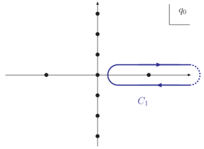
Figure 19: Integration path for Eq. (77).

The following useful formulae are easily established:

$$T\sum_{n}\frac{1}{-(i\omega_{n})^{2}+\omega_{\kappa}^{2}} = \frac{1+2n(\omega_{\kappa})}{2\omega_{\kappa}},$$ (78)

$$T\sum_{n}\frac{1}{\left(\omega_{n}^{2}+\omega_{\kappa}^{2}\right)^{2}} = \frac{1+2n_{\kappa}-2\omega_{\kappa}n^{\prime}_{\kappa}}{4\omega_{\kappa}^{3}},$$ (79)

$$T\sum_{n}\frac{1}{\left(\omega_{n}^{2}+\omega_{\kappa}^{2}\right)^{3}} = \frac{3}{16\omega_{\kappa}^{5}}\left\{1+2n_{\kappa}-2\omega_{\kappa}n^{\prime}_{\kappa}+\frac{2}{3}\omega_{\kappa}^{2}n_{\kappa}^{\prime\prime}\right\}.$$ (80)

As an application, let us derive Eq. (26) for the effective potential. Consider the longitudinal modes first. With the regulator (19) the ${\bf q}$ integration in Eq. (23) can be performed analytically, leaving

$$\partial_{\kappa}V_{\kappa}(\rho)=K_{d-1}\kappa^{d}T\sum_{n}\frac{1}{\omega_{n}^{2}+V^{\prime}_{\kappa}(\rho)+2\rho V^{\prime\prime}_{\kappa}(\rho)+\kappa^{2}}\,,$$ (81)

where $K_{d}$ is defined after Eq. (27). When $V^{\prime}_{\kappa}(\rho)+2\rho V^{\prime\prime}_{\kappa}(\rho)+\kappa^{2}>0$, we can use (78) and obtain

$$\partial_{\kappa}V_{\kappa}(\rho) = K_{d-1}\kappa^{d}\frac{2n(\omega_{\kappa}^{L})+1}{2\omega_{\kappa}^{L}}\,,$$ (82)

where $\omega_{\kappa}^{L}$ has been defined in (27). The transverse piece that leads to (26) is calculated analogously.

Appendix B Annotations to perturbative calculations

In this Appendix, we collect some technical details of the perturbative expansion of the flow equations. We will use the following results through order $g^{3}$:

The coupling at finite temperature for arbitrary soft $\kappa\leq\xi$ follows from (46) and reads at order $g^{3}$:

$$\left.g_{\kappa}^{2}\right|_{g^{3}} = \frac{9g^{3}}{\pi^{2}}\left(\arctan\frac{\kappa}{gT}-\frac{\pi}{2}-\frac{g\kappa T}{3}\frac{5\kappa^{2}+3g^{2}T^{2}}{\left(\kappa^{2}+g^{2}T^{2}\right)^{2}}+\frac{8gT}{3\xi}+O((gT/\xi)^{2})\right).$$ (83)

The thermal mass has the following behavior for small $\kappa$ which can be obtained by expanding (52) and evaluating (56) for arbitrary $\kappa$

$$\left.m_{{\rm th},\kappa}^{2}\right|_{g^{2}} = g^{2}\left(T^{2}-\frac{4T\kappa}{\pi^{2}}+\frac{\kappa^{2}}{2\pi^{2}}+O(\kappa^{5})\right),$$ (84)

$$\left.m_{{\rm th},\kappa}^{2}\right|_{g^{3}} = \frac{6g^{3}T^{2}}{\pi^{2}}\left(\arctan\frac{\kappa}{gT}-\frac{\pi}{2}-\frac{1}{3}\frac{g\kappa T}{\kappa^{2}+g^{2}T^{2}}+\frac{4gT}{3\xi}+O((gT/\xi)^{2})\right).$$ (85)

The vacuum flow $m_{{\rm vac},\kappa}^{2}$ is given in (40).

B.1 Coupling at finite temperature through order $g^{4}$

In order to calculate the constant under the logarithm of the $g^{4}$ coefficient for the thermal mass, we have to be more careful in integrating the flow equation for the coupling (31). Dividing this equation by $g_{\kappa}^{4}$ and multiplying by $d\kappa$, we can integrate the left and right hand sides of (31) independently. The r.h.s. contains IR as well as UV problems that we have to cope with. We introduce an intermediate scale $gT\ll\xi\ll T$ (e.g. $\xi\sim\sqrt{g}\,T$) and calculate this integral in two pieces. For $\kappa\geq\xi$, we can neglect $m_{\kappa}\propto gT\ll\xi$ in $\epsilon_{\kappa}$ and regulate the remaining integral by subtracting its leading divergent pieces in the IR and UV limits. Abbreviating $X(\epsilon_{\kappa})\equiv(1+2n(\epsilon_{\kappa})-2\epsilon_{\kappa}n^{\prime}(\epsilon_{\kappa})+\frac{2}{3}\epsilon_{\kappa}^{2}n^{\prime\prime}(\epsilon_{\kappa}))/{\epsilon_{\kappa}^{5}}$, we get

$$\frac{9}{2\pi^{2}}\int_{0}^{\infty}d\kappa\left[\kappa^{4}X(\kappa)-\frac{16T}{3\kappa^{2}}\theta(T-\kappa)-\frac{1}{\kappa}\theta(\kappa-T)\right]=\frac{9}{2\pi^{2}}\left(4+\gamma-\log(2\pi)\right)$$ (86)

with Euler’s constant $\gamma=0.577216$. This result is obtained by integrating those pieces of $X(\kappa)$ which contain derivatives of $n(\kappa)$ by parts and using for $n(\kappa)/\kappa$

$$\int_{0}^{\infty}\frac{d\kappa}{\kappa}\left(\frac{2}{e^{\kappa}-1}-\frac{2+\kappa}{\kappa(1+\kappa)}\right)=\gamma-\log(2\pi)$$ (87)

which can be derived by multiplying the terms by $\kappa^{a}$ and analytically continuing the result to $a\rightarrow 0$. Using (86), we can write the $\kappa\geq\xi$ contribution as

$$\frac{9}{2\pi^{2}}\int_{\xi}^{\Lambda}d\kappa\,\kappa^{4}X(\epsilon_{\kappa})=\frac{9}{2\pi^{2}}\left(\frac{16T}{\xi}+\log\frac{\Lambda}{2\pi T}+\gamma-\frac{4}{3}+O(\xi/T)\right)+O(g^{2}),$$ (88)

valid for sufficiently small $\xi\ll T$ and sufficiently large $\Lambda\gg T$.

For $\kappa\leq\xi$, we can expand $X(\epsilon_{\kappa})$ as in (44). In a first step, we use the expression (46) that leads to the $g^{3}$ contribution of the mass and expand it for large $\xi\gg gT$

$$\frac{24T}{\pi^{2}}\int_{0}^{\xi}d\kappa\frac{\kappa^{4}}{\left(\kappa^{2}+m^{2}\right)^{3}}=\frac{9T}{2\pi m}-\frac{24T}{\pi^{2}\xi}+\frac{T}{m}O((m/\xi)^{3}).$$ (89)

It is assuring that the $1/\xi$ terms cancel when adding (88) and (89), but we are still missing an $O(1)$ contribution which enters on the one hand through the missing $\kappa$ dependence of $m$ in (89), and on the other hand through the missing $g^{3}$ contribution to $m$. Both can be taken into account by replacing $m^{2}\rightarrow m_{\kappa}^{2}=m_{{\rm vac},\kappa}^{2}+\left.m_{{\rm th},\kappa}^{2}\right|_{g^{2},g^{3}}$ using (40), (84), and (85). The missing contribution can be thus calculated by

$$\lim_{g\rightarrow 0}\frac{24T}{\pi^{2}}\int_{0}^{\xi\rightarrow\infty}d\kappa\left[\frac{\kappa^{4}}{\left(\kappa^{2}+m_{\kappa}^{2}\right)^{3}}-\frac{\kappa^{4}}{\left(\kappa^{2}+g^{2}T^{2}\right)^{3}}\right]\!\!\!\!\!\!\!\!\!\!\!\!\!\!\!\!\!\!\!\!\!\!\!\!\!\!\!\!\!\!\!\!\!\!\!\!\!\!\!\!\!\!\!\!\!\!\!\!\!\!\!\!\!\!\!\!\!\!\!\!\!\!\!\!\!\!\!\!\!\!\!\!\!\!\!\!\!\!\!\!\!\!\!\!\!\!\!\!\!\!\!\!\!\!\!\!\!\!\!\!\!\!\!\!\!\!\!\!\!\!\!\!$$ (90)

$$= \frac{432T^{2}}{{\pi}^{4}}\int_{0}^{\infty}d\bar{\kappa}\frac{{\bar{\kappa}}^{4}}{\left(T^{2}+\bar{\kappa}^{2}\right)^{5}}\left(-\frac{{\bar{\kappa}}^{3}}{3}+T\left(T^{2}+{\bar{\kappa}}^{2}\right)\left(\frac{\pi}{2}+\frac{\bar{\kappa}}{T}-\arctan(\frac{\bar{\kappa}}{T})\right)\right)+O(g)$$

$$= \frac{48}{{\pi}^{4}}+\frac{27}{8\pi^{2}}+O(g),$$

where we have expanded the first denominator around $\kappa^{2}+g^{2}T^{2}$ and substituted $\bar{\kappa}=\kappa/g$ to form the $g\rightarrow 0$ limit.

We obtain the final result by combining (88) + (89) + (90):

$$\frac{9}{2\pi^{2}}\int_{0}^{\Lambda}d\kappa\,\kappa^{4}X(\epsilon_{\kappa}) = \frac{9}{2\pi^{2}}\left(\frac{\pi}{g}+\log\frac{\Lambda}{2\pi T}+\gamma-\frac{7}{12}+\frac{32}{3\pi^{2}}\right)+O(g)$$ (91)

Inserting this result into (31), we obtain

$$\frac{1}{g_{0}^{2}}-\frac{1}{g_{\Lambda}^{2}}=\frac{9}{2\pi g_{\Lambda}}+\frac{9}{2\pi^{2}}\left(\log\frac{\Lambda}{2\pi T}+\gamma-\frac{7}{12}+\frac{32}{3\pi^{2}}\right)+O(g_{\Lambda}),$$ (92)

or, expanding and using (10) to change from $g_{\Lambda}$ to $g_{\kappa}$ for $T\lesssim\kappa\leq\Lambda$, we obtain

$$g_{0}^{2}=g_{\kappa}^{2}-\frac{9g_{\kappa}^{3}}{2\pi}-\frac{9g_{\kappa}^{4}}{2\pi^{2}}\left(\log\frac{\kappa}{2\pi T}+\gamma-\frac{61}{12}+\frac{32}{3{\pi}^{2}}\right)+O(g_{\kappa}^{5}),$$ (93)

which connects the value of the coupling at $\kappa=0$ to the value of the coupling $\kappa\gtrsim T$.

B.2 Thermal mass through order $g^{4}\ln g$

When deriving the thermal mass at order $g^{3}$, in (56) we had neglected the flow of $g_{\kappa}$ and $m_{\kappa}$ at order $g^{3}$ which may change the result of the mass at order $g^{3}$. We will see that in the IR region $\kappa\leq\xi$ (with $gT\ll\xi\ll T$) such corrections would only affect the result at order $g^{4}\ln g$, thereby justifying the IR calculation (56). In the UV region $\kappa\geq\xi$ on the other hand, these corrections would affect the result only at order $g^{4}$, thereby establishing (56) not only as the correct result for the IR, but for all $\kappa$ at order $g^{3}$.

The $g^{3}$ correction to the coupling only affects $g_{\kappa}$ in the first line of Eq. (55). We can therefore expand $g_{\kappa}^{2}\rightarrow g^{2}+\delta g_{\kappa}^{2}$ with $\delta g_{\kappa}^{2}=g_{\kappa}^{2}|_{g^{3}}$ from (83). (The $g^{2}$ in the second line of (55) is not affected by this, as we subtract a clean $g^{2}$ contribution.) In the region $\kappa\leq\xi$, we can expand the thermal distribution function in (55). The correction to (56) is then given by

$$\frac{4T}{\pi^{2}}\int_{0}^{\xi}d\kappa\,\delta g_{\kappa}^{2}\frac{\kappa^{4}}{(\kappa^{2}+m^{2})^{2}}=\frac{96g^{4}T^{2}}{\pi^{4}}\left(\log\frac{gT}{\xi}+\frac{25}{24}+\frac{9\pi^{2}}{128}-\frac{3\pi gT}{4\xi}+O((gT/\xi)^{2})\right).$$ (94)

This contribution is of the order $g^{4}\ln g$. We expect the $\log(gT/\xi)$ from the IR region $\kappa\leq\xi$ to combine with a corresponding $\log(\xi/T)$ in the UV region $\kappa\geq\xi$, but this calculation is beyond the scope of this paper. Since $g^{3}$ corrections to the coupling and mass are IR results stemming from $\kappa\leq\xi$, it is clear that no further $g^{3}$ contribution can build up in the UV. Therefore, there can not be any additional correction to the thermal mass, and (56) already captures the full $g^{3}$ term.

References

- Blaizot et al. (2003a) J.-P. Blaizot, E. Iancu, and A. Rebhan, in Hwa, R.C. (ed.) et al.: Quark gluon plasma 60-122 (2003a), eprint hep-ph/0303185.
- Arnold and Zhai (1995) P. Arnold and C.-X. Zhai, Phys. Rev. D51, 1906 (1995), eprint hep-ph/9410360.
- Zhai and Kastening (1995) C.-X. Zhai and B. Kastening, Phys. Rev. D52, 7232 (1995), eprint hep-ph/9507380.
- Braaten and Nieto (1996) E. Braaten and A. Nieto, Phys. Rev. D53, 3421 (1996), eprint hep-ph/9510408.
- Kajantie et al. (2003) K. Kajantie, M. Laine, K. Rummukainen, and Y. Schröder, Phys. Rev. D67, 105008 (2003), eprint hep-ph/0211321.
- Di Renzo et al. (2006) F. Di Renzo, M. Laine, V. Miccio, Y. Schroder, and C. Torrero (2006), eprint hep-ph/0605042.
- Parwani and Singh (1995) R. Parwani and H. Singh, Phys. Rev. D51, 4518 (1995), eprint hep-th/9411065.
- Drummond et al. (1998) I. T. Drummond, R. R. Horgan, P. V. Landshoff, and A. Rebhan, Nucl. Phys. B524, 579 (1998), eprint hep-ph/9708426.
- Karsch et al. (1997) F. Karsch, A. Patkós, and P. Petreczky, Phys. Lett. B401, 69 (1997), eprint hep-ph/9702376.
- Andersen et al. (2001) J. O. Andersen, E. Braaten, and M. Strickland, Phys. Rev. D63, 105008 (2001), eprint hep-ph/0007159.
- Andersen et al. (1999) J. O. Andersen, E. Braaten, and M. Strickland, Phys. Rev. Lett. 83, 2139 (1999), eprint hep-ph/9902327.
- Andersen et al. (2002) J. O. Andersen, E. Braaten, E. Petitgirard, and M. Strickland, Phys. Rev. D66, 085016 (2002), eprint [http://arXiv.org/abs]hep-ph/0205085.
- Andersen et al. (2004) J. O. Andersen, E. Petitgirard, and M. Strickland, Phys. Rev. D70, 045001 (2004), eprint hep-ph/0302069.
- Andersen and Strickland (2005) J. O. Andersen and M. Strickland, Ann. Phys. 317, 281 (2005), eprint hep-ph/0404164.
- Blaizot et al. (1999a) J.-P. Blaizot, E. Iancu, and A. Rebhan, Phys. Rev. Lett. 83, 2906 (1999a), eprint hep-ph/9906340.
- Blaizot et al. (1999b) J.-P. Blaizot, E. Iancu, and A. Rebhan, Phys. Lett. B470, 181 (1999b), eprint hep-ph/9910309.
- Blaizot et al. (2001) J.-P. Blaizot, E. Iancu, and A. Rebhan, Phys. Rev. D63, 065003 (2001), eprint hep-ph/0005003.
- Luttinger and Ward (1960) J. M. Luttinger and J. C. Ward, Phys. Rev. 118, 1417 (1960).
- Baym (1962) G. Baym, Phys. Rev. 127, 1391 (1962).
- Cornwall et al. (1974) J. M. Cornwall, R. Jackiw, and E. Tomboulis, Phys. Rev. D10, 2428 (1974).
- Vanderheyden and Baym (1998) B. Vanderheyden and G. Baym, J. Stat. Phys. 93, 843 (1998), eprint hep-ph/9803300.
- Kajantie et al. (2001) K. Kajantie, M. Laine, K. Rummukainen, and Y. Schroder, Phys. Rev. Lett. 86, 10 (2001), eprint [http://arXiv.org/abs]hep-ph/0007109.
- Braaten and Nieto (1995) E. Braaten and A. Nieto, Phys. Rev. D51, 6990 (1995), eprint hep-ph/9501375.
- Blaizot et al. (2003b) J.-P. Blaizot, E. Iancu, and A. Rebhan, Phys. Rev. D68, 025011 (2003b), eprint hep-ph/0303045.
- Wetterich (1993) C. Wetterich, Phys. Lett. B301, 90 (1993).
- Ellwanger (1993) U. Ellwanger, Z. Phys. C58, 619 (1993).
- Tetradis and Wetterich (1994) N. Tetradis and C. Wetterich, Nucl. Phys. B422, 541 (1994), eprint hep-ph/9308214.
- Morris (1994a) T. R. Morris, Int. J. Mod. Phys. A9, 2411 (1994a), eprint hep-ph/9308265.
- Morris (1994b) T. R. Morris, Phys. Lett. B329, 241 (1994b), eprint hep-ph/9403340.
- Delamotte et al. (2004) B. Delamotte, D. Mouhanna, and M. Tissier, Phys. Rev. B69, 134413 (2004), eprint cond-mat/0309101.
- Delamotte and Canet (2005) B. Delamotte and L. Canet, Condensed Matter Phys. 8, 163 (2005), eprint cond-mat/0412205.
- Ellwanger (1994) U. Ellwanger, Z. Phys. C62, 503 (1994), eprint hep-ph/9308260.
- Ellwanger and Wetterich (1994) U. Ellwanger and C. Wetterich, Nucl. Phys. B423, 137 (1994), eprint hep-ph/9402221.
- Ellwanger et al. (1998) U. Ellwanger, M. Hirsch, and A. Weber, Eur. Phys. J. C1, 563 (1998), eprint hep-ph/9606468.
- Pawlowski et al. (2004) J. M. Pawlowski, D. F. Litim, S. Nedelko, and L. von Smekal, Phys. Rev. Lett. 93, 152002 (2004), eprint hep-th/0312324.
- Fischer and Gies (2004) C. S. Fischer and H. Gies, JHEP 10, 048 (2004), eprint hep-ph/0408089.
- Arnone et al. (2005) S. Arnone, T. R. Morris, and O. J. Rosten (2005), eprint hep-th/0507154.
- Morris and Rosten (2006) T. R. Morris and O. J. Rosten, J. Phys. A39, 11657 (2006), eprint hep-th/0606189.
- Bagnuls and Bervillier (2001) C. Bagnuls and C. Bervillier, Phys. Rept. 348, 91 (2001), eprint hep-th/0002034.
- Berges et al. (2002) J. Berges, N. Tetradis, and C. Wetterich, Phys. Rept. 363, 223 (2002), eprint hep-ph/0005122.
- Pawlowski (2005) J. M. Pawlowski (2005), eprint hep-th/0512261.
- Reuter et al. (1993) M. Reuter, N. Tetradis, and C. Wetterich, Nucl. Phys. B401, 567 (1993), eprint hep-ph/9301271.
- Andersen and Strickland (1999) J. O. Andersen and M. Strickland, Phys. Rev. A60, 1442 (1999), eprint cond-mat/9811096.
- D’Attanasio and Pietroni (1996) M. D’Attanasio and M. Pietroni, Nucl. Phys. B472, 711 (1996), eprint hep-ph/9601375.
- Liao and Strickland (1995) S.-B. Liao and M. Strickland, Phys. Rev. D52, 3653 (1995), eprint hep-th/9501137.
- Braun et al. (2004) J. Braun, K. Schwenzer, and H.-J. Pirner, Phys. Rev. D70, 085016 (2004), eprint hep-ph/0312277.
- Blaizot (2006a) J.-P. Blaizot, International Conference on Strong & Electroweak Matter, Nucl. Phys. A, BNL, May 10-13 (2006a).
- Blaizot (2006b) J.-P. Blaizot, “RHIC Physics in the Context of the Standard model”, in the proceedings of RIKEN BNL Research Center Workshop, Vol. 82, June 18-23 (2006b).
- Arnold and Zhai (1994) P. Arnold and C.-X. Zhai, Phys. Rev. D50, 7603 (1994), eprint hep-ph/9408276.
- Blaizot et al. (2004) J.-P. Blaizot, E. Iancu, and U. Reinosa, Nucl. Phys. A736, 149 (2004), eprint hep-ph/0312085.
- Ringwald and Wetterich (1990) A. Ringwald and C. Wetterich, Nucl. Phys. B334, 506 (1990).
- Bervillier (2005) C. Bervillier (2005), eprint hep-th/0501087.
- Ball et al. (1995) R. D. Ball, P. E. Haagensen, I. Latorre, Jose, and E. Moreno, Phys. Lett. B347, 80 (1995), eprint hep-th/9411122.
- Comellas (1998) J. Comellas, Nucl. Phys. B509, 662 (1998), eprint hep-th/9705129.
- Liao et al. (2000) S.-B. Liao, J. Polonyi, and M. Strickland, Nucl. Phys. B567, 493 (2000), eprint hep-th/9905206.
- Litim (2000) D. F. Litim, Phys. Lett. B486, 92 (2000), eprint hep-th/0005245.
- Litim (2001a) D. F. Litim, Phys. Rev. D64, 105007 (2001a), eprint hep-th/0103195.
- Polchinski (1984) J. Polchinski, Nucl. Phys. B231, 269 (1984).
- Litim (2001b) D. F. Litim, Int. J. Mod. Phys. A16, 2081 (2001b), eprint hep-th/0104221.
- Canet et al. (2003a) L. Canet, B. Delamotte, D. Mouhanna, and J. Vidal, Phys. Rev. D67, 065004 (2003a), eprint hep-th/0211055.
- Tetradis and Wetterich (1993) N. Tetradis and C. Wetterich, Nucl. Phys. B398, 659 (1993).
- Morris (1994c) T. R. Morris, Phys. Lett. B334, 355 (1994c), eprint hep-th/9405190.
- Canet et al. (2003b) L. Canet, B. Delamotte, D. Mouhanna, and J. Vidal, Phys. Rev. B68, 064421 (2003b), eprint hep-th/0302227.
- D’Attanasio and Morris (1997) M. D’Attanasio and T. R. Morris, Phys. Lett. B409, 363 (1997), eprint hep-th/9704094.
- Tetradis and Litim (1996) N. Tetradis and D. F. Litim, Nucl. Phys. B464, 492 (1996), eprint hep-th/9512073.
- Blaizot and Reinosa (2006) J.-P. Blaizot and U. Reinosa, Nucl. Phys. A764, 393 (2006), eprint hep-ph/0406109.
- Blaizot et al. (2003c) J.-P. Blaizot, R. Mendez-Galain, and N. Wschebor, Ann. Phys. 307, 209 (2003c), eprint hep-ph/0212084.
- Blaizot et al. (2005) J.-P. Blaizot, R. Mendez-Galain, and N. Wschebor (2005), eprint hep-th/0512317.
- Blaizot et al. (2006a) J.-P. Blaizot, R. Mendez-Galain, and N. Wschebor (2006a), eprint hep-th/0603163.
- Blaizot et al. (2006b) J.-P. Blaizot, R. Mendez Galain, and N. Wschebor, Phys. Lett. B632, 571 (2006b), eprint hep-th/0503103.
- Blaizot et al. (2006c) J.-P. Blaizot, R. Mendez-Galain, and N. Wschebor (2006c), eprint hep-th/0605252.
- Vermaseren (1994) J. A. M. Vermaseren, Comput. Phys. Commun. 83, 45 (1994).
- Binosi and Theussl (2004) D. Binosi and L. Theussl, Comput. Phys. Commun. 161, 76 (2004), eprint hep-ph/0309015.
- Litim and Pawlowski (2006) D. F. Litim and J. M. Pawlowski (2006), eprint hep-th/0609122.