Kaonic Quantum Erasers at KLOE $2$:
“Erasing the Present, changing the Past”

Abstract

Neutral kaons are unique quantum systems to show some of the most puzzling peculiarities of quantum mechanics. Here we focus on a quantitative version of Bohr’s complementary principle and on quantum marking and eraser concepts. In detail we show that neutral kaons $(1)$ are kind of double slit devices encapsulating Bohr’s complementarity principle in a simple and transparent way, and $(2)$ offer marking and eraser options which are not afforded by other quantum systems and which can be performed at the DA$\Phi$NE machine.

1 Introduction

During the last fifteen years or so we have witnessed an interesting revival of the research concerning some fundamental issues of quantum mechanics. A very positive aspect of this revival is that it has been driven by a series of impressive results which have been possible thanks to improved experimental techniques and skillful ideas of several experimental groups. As a result, some of the Gedankenexperimente proposed and discussed in the earlier days of quantum mechanics, or slight modifications of these proposals, have been finally performed in the laboratory. Most of these experiments belong to the fields of quantum optics and photonics; others make use of (single) atomic or ion states.

Among these kinds of experiments we concentrate on two types. The first type concerns the old complementarity principle of Niels Bohr for which a quantitative version became available in recent years. This ‘quantitative complementarity’ represents a major improvement over older treatments and can be tested for rather simple quantum systems. The second type of experiments requires more complex states consisting of entangled two–particle systems. With these bipartite states at hand one can test much more subtle quantum phenomena such as the so called ‘quantum eraser’, which adds puzzling space–time considerations to the previous, Bohr’s complementarity issue.

The aim of our contribution is to analyze the role that neutral kaons can play in this two types of experiments. A copious source of entangled neutral meson pairs, such as those produced in the Daphne $e^{+}e^{-}$ machine, can be shown to be extremely useful for this purpose.

2 Kaons as double slits

The famous statement about quantum mechanics “the double slit contains the only mystery” of Richard Feynman is well known, his statement about neutral kaons is not less to the point: “If there is any place where we have a chance to test the main principles of quantum mechanics in the purest way —does the superposition of amplitudes work or doesn’t it?— this is it” [1]. In this section we argue that single neutral kaons can be considered as double slits as well.

Bohr’s complementarity principle and the closely related concept of duality in interferometric or double–slit like devices are at the heart of quantum mechanics. The well–known qualitative statement that “the observation of an interference pattern and the acquisition of which–way information are mutually exclusive” has only recently been rephrased to a quantitative statement [2, 3]:

$${\cal P}^{2}(y)+{\cal V}_{0}^{2}(y)\leq 1\;,$$ (1)

where the equality is valid for pure quantum states and the inequality for mixed ones. ${\cal V}_{0}(y)$ is the fringe visibility, which quantifies the sharpness or contrast of the interference pattern (the “wave–like” property), whereas ${\cal P}(y)$ denotes the path predictability, i.e., the a priori knowledge one can have on the path taken by the interfering system (the “particle–like” property). The path predictability is defined by [2]

$${\cal P}(y)\;=\;|p_{I}(y)-p_{II}(y)|\;,$$ (2)

where $p_{I}(y)$ and $p_{II}(y)$ are the probabilities for taking each path ($p_{I}(y)+p_{II}(y)=1)$. Both ${\cal V}_{0}(y)$ and ${\cal P}(y)$ depend on the same parameter $y$ related somehow to the geometry of the interferometric setup. It is often too idealized to assume that the predictability and visibility are independent of this external parameter $y$. For example, consider a usual experiment with a vertical screen having a higher and a lower slit. Then the intensity is generally given by

$$I(y)\;=\;F(y)\;\big{(}1+{\cal V}_{0}(y)\cos(\phi(y)\big{)}\;,$$ (3)

where $F(y)$ is specific for each setup and $\phi(y)$ is the phase–difference between the two paths. The variable $y$ characterizes in this case the position of the detector scanning a vertical plane beyond the double–slit. An accurate description of the interference pattern, whose contrast along a wide scanned region can hardly be constant, thus requires to consider the $y$–dependence of visibility and predictability.

In Ref. [4] the authors investigated physical situations for which the expressions of ${\cal V}_{0}(y),{\cal P}(y)$ and $\phi(y)$ can be calculated analytically. This included interference patterns of various types of double slit experiments ($y$ is linked to position), as well as Mott scattering experiments of identical particles or nuclei ($y$ is linked to a scattering angle). But it also included particle–antiparticle oscillations in time due to particle mixing, as in the neutral kaon system. In this case, $y$ is a time variable indirectly linked to the position of the kaon detector or the kaon decay vertex. Remarkably, all these two–state systems, belonging to quite distinct fields of physics, can then be treated via the generalized complementarity relation (1) in a unified way. Even for specific thermodynamical systems, Bohr’s complementarity can manifest itself, see Ref. [5]. Here we investigate the neutral kaon case.

The time evolution of an initial $K^{0}$ state is given by

$$|K^{0}(t)\rangle = \frac{1}{\sqrt{2}}e^{-im_{L}t-\frac{\Gamma_{L}}{2}t}\left\{e^{i\Delta mt+\frac{\Delta\Gamma}{2}t}\,|K_{S}\rangle+|K_{L}\rangle\right\}\;,$$ (4)

where (here and in the following) inessential $CP$ violation effects are safely neglected. In our notation $\Delta m\equiv m_{L}-m_{S}$ is the (small) mass difference between the long– and short–lived kaon components whose time evolution is simply given by

$$|K_{S}(t)\rangle=e^{-im_{S}t}e^{-{1\over 2}\Gamma_{S}t}\,|K_{S}\rangle\;,\>\;|K_{L}(t)\rangle=e^{-im_{L}t}e^{-{1\over 2}\Gamma_{L}t}\,|K_{L}\rangle\;.$$ (5)

Note that there are no oscillations in time between these two states and that their decay rates are remarkably different, $\Gamma_{S}\simeq 579\Gamma_{L}$, so that we can write $\Delta\Gamma\equiv\Gamma_{L}-\Gamma_{S}\simeq-\Gamma_{S}\simeq-2.1\Delta m<0$.

State (4) can be interpreted as follows. The two mass eigenstates $|K_{S}\rangle$ and $|K_{L}\rangle$, i.e. the two terms in the right hand side of eq. (4), represent the two slits. At time $t=0$ both terms (slits) have the same weight (width) and constructively interfere with a common phase. As time evolves, the $K_{S}$ component decreases faster than the other one and this can be interpreted as a relative shrinkage of the $K_{S}$–slit making more likely the ‘passage’ through the $K_{L}$–slit. In addition, the norm of eq. (4) decreases with time as a consequence of both $K_{S}$ and $K_{L}$ decays, an effect which could be mimicked by an hypothetical shrinkage of both slit widths in real double–slit experiments. The analogy gets more obvious if we eliminate this latter effect by restricting to kaons which survive up to a certain time $t$ and are thus described by renormalizing the state (4):

$$|K^{0}(t)\rangle \cong \frac{1}{\sqrt{2\cosh(\frac{\Delta\Gamma}{2}t)}}\;e^{-\frac{\Delta\Gamma}{4}t}\left\{e^{i\Delta mt+\frac{\Delta\Gamma}{2}t}\,|K_{S}\rangle+|K_{L}\rangle\right\}\;.$$ (6)

The probabilities for detecting on this state either a $K^{0}$ or a $\bar{K}^{0}$ are given by

$$P(K^{0},t) = \left|\langle K^{0}|K^{0}(t)\rangle\right|^{2}=\frac{1}{2}\biggl{\{}1+\frac{\cos(\Delta mt)}{\cosh(\frac{\Delta\Gamma}{2}t)}\biggr{\}}$$

$$P(\bar{K}^{0},t) = \left|\langle\bar{K}^{0}|K^{0}(t)\rangle\right|^{2}=\frac{1}{2}\biggl{\{}1-\frac{\cos(\Delta mt)}{\cosh(\frac{\Delta\Gamma}{2}t)}\biggr{\}}\;,$$ (7)

showing the well–known strangeness oscillations. We observe that the oscillating phase is given by $\phi(t)=\Delta m\,t$ and the time dependent visibility by

$${\cal V}_{0}(t)=\frac{1}{\cosh(\frac{\Delta\Gamma}{2}t)}\;.$$ (8)

The path predictability ${\cal P}(t)$, which in our kaonic case corresponds to a “which width” information, can be directly calculated from eq. (6)

$${\cal P}(t)=\left|P(K_{S},t)-P(K_{L},t)\right|=\left|\;\frac{e^{\frac{\Delta\Gamma}{2}t}\;-\;e^{-\frac{\Delta\Gamma}{2}t}}{2\cosh(\frac{\Delta\Gamma}{2}t)}\;\right|=\left|\;\tanh\big{(}\frac{\Delta\Gamma}{2}t\big{)}\right|\;.$$ (9)

The expressions for predictability (9) and visibility (19) satisfy the complementary relation (1) for all times $t$

$${\cal P}^{2}(t)+{\cal V}_{0}^{2}(t)\;=\;\tanh^{2}\big{(}\frac{\Delta\Gamma}{2}t\big{)}+\frac{1}{\cosh^{2}(\frac{\Delta\Gamma}{2}t)}\>=\;1\;.$$ (10)

For time $t=0$ there is full interference, the visibility is maximal, ${\cal V}_{0}(t=0)=1$, and we have no information about the lifetime, ${\cal P}(t=0)=0$. This corresponds to the central part (around the zero–order maximum) of the interference pattern in a usual double slit scenario. For very large times, i.e. $t\gg 1/\Gamma_{S}$, the surviving kaon is most probably in a long lived state $K_{L}$ and no interference is observed since we have almost perfect information on “which width” is actually propagating. For times between these two extremes and due to the natural instability of the kaons, we obtain partial “which width” information and the expected interference contrast is thus smaller than one. However, the full information on the system is contained in eq. (1) and is always maximal for pure states.

The complementarity principle was proposed by Niels Bohr in an attempt to express the most fundamental difference between classical and quantum physics. According to this principle, and in sharp contrast to classical physics, in quantum physics we cannot capture all aspects of reality simultaneously and the available information on complementary aspects is always limited. Neutral kaons encapsulate indeed this peculiar feature in the very same way as a particle having passed through a double slit. But kaons are double slit devices automatically provided by Nature for free!

3 Kaonic quantum eraser

Two hundred years ago Thomas Young taught us how to observe interference phenomena with light beams. Much more later, interference effects of light have been observed at the single photon level. Nowadays also experiments with very massive particles, like fullerene molecules, have impressively demonstrated that fundamental feature of quantum mechanics [6]. It seems that there is no physical reason why not even heavier particles should interfere except for technical ones. In the previous section we have shown that interference effects disappear if it is possible to know the path through the double slit. The ‘quantum eraser’, a gedanken experiment proposed by Scully and Drühl in 1982 [7], surprised the physics community: if that knowledge on the path of the particle is erased, interference can be brought back again.

Since that work many different types of quantum erasers have been analyzed and experiments have been performed with atom interferometers [8] and with entangled photon pairs [9, 10, 12, 13, 14, 15]. In most of them, the quantum erasure is performed in the so-called “delayed choice” mode which best captures the essence and the most subtle aspects of the eraser phenomenon. In this case the meter, the quantum system which carries the mark on the path taken, is a system spatially separated from the interfering system which is generally called the object system. The decision to erase or not the mark of the meter system —and therefore the possibility to observe or not interference— can be taken long after the measurement on the object system has been completed. This was nicely phrased by Aharonov and Zubairy in the title of their review article [16] as “erasing the past and impacting the future”.

Here we want to present four conceptually different types of quantum erasers for neutral kaons, Refs. [17, 18]. Two of them are analogous to erasure experiments already performed with entangled photons, e.g. Refs. [9, 10]. For convenience of the reader we added two figures sketching the setups of these experiments, Fig. 1 and Fig. 2. In the first experiment the erasure operation was carried out “actively”, i.e., by exerting the free will of the experimenter, whereas in the latter experiment the erasure operation was carried out “partially actively”, i.e., the mark of the meter system was erased or not by a well known probabilistic law: photon reflection or transmission in a beam splitter. However, different to photons the kaons can be measured by an active or a completely passive procedure. This offers new quantum erasure possibilities and proves the underlying working principle of a quantum eraser, namely, sorting events according to the acquired information.

For neutral kaons there exist two relevant alternative physical bases. The first basis is the strangeness eigenstate basis $\{|K^{0}\rangle,|\bar{K}^{0}\rangle\}$. The strangeness $S$ of an incoming neutral kaon at a given time $t$ can be measured by inserting at the appropriate point of the kaon trajectory a thin piece of high–density matter. Due to strangeness conservation of the strong interactions between kaons and nucleons, the incoming state is projected either onto $K^{0}$, by a reaction like $K^{0}p\rightarrow K^{+}n$, or onto $\bar{K}^{0}$, by other reactions such as $\bar{K}^{0}p\rightarrow\Lambda\pi^{+}$, $\bar{K}^{0}n\rightarrow\Lambda\pi^{0}$ or $\bar{K}^{0}n\rightarrow K^{-}p$. Here the nucleonic matter plays the same role as a two channel analyzer for polarized photon beams. We refer to this kind of strangeness measurement, which requires the insertion of that piece of matter, as an active measurement.

Alternatively, the strangeness content of neutral kaons can be determined by observing their semileptonic decay modes. Indeed, these semileptonic decays obey the well tested $\Delta S=\Delta Q$ rule which allows the modes

$$K^{0}(\bar{s}d)\to\pi^{-}(\bar{u}d)\;+\;l^{+}\;+\;\nu_{l}\;,\;\;\bar{K}^{0}(s\bar{d})\to\pi^{+}(u\bar{d})\;+\;l^{-}\;+\;\bar{\nu}_{l},$$ (11)

where $l$ stands for $e$ or $\mu$, but forbids decays into the respective charge conjugated modes. Obviously, the experimenter has no control on the kaon decay, neither on the mode nor on the time. The experimenter can only sort the set of all observed events in proper decay modes and time intervals. We call this procedure, opposite to the active measurement procedure described above, a passive strangeness measurement.

The second basis $\{K_{S},K_{L}\}$ consists of the short– and long–lived states having well defined masses $m_{S(L)}$ and decay widths $\Gamma_{(S)L}$. We have seen that it is the appropriate basis to discuss the kaon propagation in free space because these states preserve their own identity in time, eq. (5). Due to the huge difference in the decay widths, the $K_{S}$’s decay much faster than the $K_{L}$’s. Thus in order to observe if a propagating kaon is a $K_{S}$ or $K_{L}$ at an instant time $t$, one has to detect at which time it subsequently decays. Kaons which are observed to decay before $\simeq t+4.8\,\tau_{S}$ have to be identified as $K_{S}$’s, while those surviving after this time are assumed to be $K_{L}$’s. Misidentifications reduce only to a few parts in $10^{-3}$, see also Refs. [17, 18]. Note that the experimenter doesn’t care about the specific decay mode, he has to allow for free propagation and to record only the time of each decay event. We call this procedure an active measurement of lifetime. Indeed, it is by actively placing or removing an appropriate piece of matter that the strangeness (as previously discussed) or the lifetime of a given kaon can be measured. Since one measurement excludes the other, the experimenter has to decide which one is actually performed and the kind of information thus obtained.

On the other hand, neglecting $CP$ violation effects —recall that they are of the order of $10^{-3}$, like the just mentioned $K_{S},K_{L}$ misidentifications— the $K_{S}$’s can be also identified by their specific decay into $2\pi$ final states ($CP=+$), while $3\pi$ final states ($CP=-$) have to be associated with $K_{L}$ decays. As before, we call this procedure a passive measurement of lifetime, since the kaon decay times and decay channels (two vs three pions) used in the measurement are entirely determined by the quantum nature of kaons and cannot be in any way influenced by the experimenter.

      (a) Active eraser with active measurements

Let us first discuss the quantum eraser experiments performed with photon pairs in Ref. [9]. In this experiment (see Fig. 1) two interfering two–photon amplitudes are prepared by forcing a pump beam to cross twice the same nonlinear crystal. Idler and signal photons from the first down conversion are marked by subsequently rotating their polarization by $90^{\circ}$ and then superposed to the idler (i) and signal (s) photons emerging from the second passage of the beam through the same crystal. If type–II spontaneous parametric down conversion were used, we would had the two–photon state

$$|\psi\rangle = \frac{1}{\sqrt{2}}\biggl{\{}\underbrace{|V\rangle_{i}|H\rangle_{s}}_{\rm{second\;passage}}-\,e^{i\Delta\phi}\,\underbrace{|H\rangle_{i}|V\rangle_{s}}_{\rm{first\;passage}}\biggr{\}}\;,$$ (12)

where $H$ and $V$ refer to horizontal and vertical polarizations The first and second terms in Eq. (12) correspond to pair production at the second and first passage of the pump beam. Their relative phase $\Delta\phi$, which depends on the difference between the paths, is thus under control by the experimenter. The signal photon, the object system, is always measured by means of a two–channel polarization analyzer aligned at $+45^{0}$. Due to entanglement, the vertical or horizontal idler polarization supplies full which way information for the signal system, i.e., whether it was produced at the first or second passage. In this first experimental setup, where nothing is made to erase the polarization marks, no interference can be observed in the signal–idler joint detections. To erase this information, the idler photon has to be detected also in the $+45^{\circ}/-45^{\circ}$ basis. This is simply achieved in a second setup by changing the orientation of the half–wave plate in the meter path. Interference fringes or, more precisely, fringes and anti–fringes can then be observed in each one of the two channels when the relative phase $\Delta\phi$ is modified.

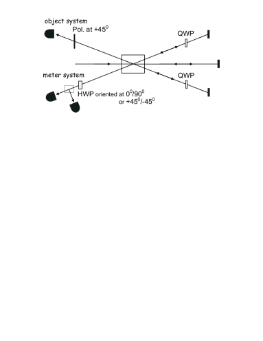
Figure 1: Sketched setup for an active eraser. A bump beam transverses twice a non–linear crystal producing photon pairs by (type II) parametric down–conversion. The pairs produced in the first passage through the crystal (from left to right) cross two times twice a quarter–wave plate (QWP) which transforms an original horizontal polarized photon into a vertical one and vice versa. The pairs produced in the second passage through the crystal (from right to left) are superposed to the previous ones and directed to the measurement devices. The signal or object photon is always detected after crossing a polarization analyzer aligned at $+45^{\circ}$. The idler or meter photon crosses a half–wave plate (HWP) oriented at $0^{\circ},90^{\circ}$ (first setup) or at $\pm 45^{\circ}$ (second setup) and is then analyzed by a polarization beam splitter. In the first setup —the meter photon is measured in the $H/V$ basis— one has full which way information, namely, one knows that the pair was produced at the first or second passage. In the second setup —the meter photon is measured in the $+45^{\circ}/-45^{\circ}$ basis— the information on the first or second passage is erased. One then observes fringes for one–half of the joint detections and the complementary (anti-)fringes for the other half.

In the case of entangled kaons produced by $\phi$ resonance decays one starts with the state

$$|\phi(0)\rangle=\frac{1}{\sqrt{2}}\left[|K^{0}\rangle_{l}|\bar{K}^{0}\rangle_{r}-|\bar{K}^{0}\rangle_{l}|K^{0}\rangle_{r}\right]\simeq\frac{1}{\sqrt{2}}\left[|K_{L}\rangle_{l}|K_{S}\rangle_{r}-|K_{S}\rangle_{l}|K_{L}\rangle_{r}\right],$$ (13)

where the $l$ and $r$ subscripts denote the “left” and “right” directions of motion of the two separating kaons and, as before, CP–violating effects are neglected in the last equality. Kaons evolve in time in such a way that the relevant state turns out to depend on the two measurement times, $t_{l}$ and $t_{r}$, on the left and the right hand side, respectively. More conveniently, this two–kaon state can be made to depend only on $\Delta t=t_{l}-t_{r}\,$ by normalizing to surviving kaon pairs

$$|\phi(\Delta t)\rangle = \frac{1}{\sqrt{1+e^{\Delta\Gamma\Delta t}}}\biggl{\{}|K_{L}\rangle_{l}|K_{S}\rangle_{r}-e^{i\Delta m\Delta t}e^{{1\over 2}\Delta\Gamma\Delta t}|K_{S}\rangle_{l}|K_{L}\rangle_{r}\biggr{\}}$$

$$= \frac{1}{2\sqrt{1+e^{\Delta\Gamma\Delta t}}}\left\{\big{(}1-e^{i\Delta m\Delta t}e^{{1\over 2}\Delta\Gamma\Delta t}\big{)}\{|K^{0}\rangle_{l}|K^{0}\rangle_{r}-|\bar{K}^{0}\rangle_{l}|\bar{K}^{0}\rangle_{r}\}\right.$$

$$\hphantom{\frac{1}{2\sqrt{1+e^{\Delta\Gamma\Delta t}}}}\left.+\big{(}1+e^{i\Delta m\Delta t}e^{{1\over 2}\Delta\Gamma\Delta t}\big{)}\{|K^{0}\rangle_{l}|\bar{K}^{0}\rangle_{r}-|\bar{K}^{0}\rangle_{l}|K^{0}\rangle_{r}\}\right\}.$$

We note that the phase $\Delta m\Delta t$ introduces automatically a time dependent relative phase between the two amplitudes. Moreover, there is a complete analogy between the photonic state (12) and the two–kaon state written in the lifetime basis, first eq. (3).

The marking and erasure operations can be performed on entangled kaon pairs (3) as in the optical case discussed above. The object kaon flying to the left hand side is measured always actively in the strangeness basis, see Fig. 3(a). This active measurement is performed by placing the strangeness detector at different points of the left trajectory, thus searching for oscillations along a certain $t_{l}$ range. As in the optical version, the kaon flying to the right hand side, the meter kaon, is always measured actively at a fixed time $t_{r}^{0}$. But one chooses to make this measurement either in the strangeness basis by placing a piece of matter in the beam or in the lifetime basis by removing the piece of matter. Both measurements are thus performed actively. In the latter case we obtain full information about the lifetime of the meter kaon and, thanks to the entanglement, which width the object kaon has. Consequently, no interference in the meter–object joint detections can be observed. This can be immediately seen from eq. (3) once the left and right kaon kets are written in the strangeness and lifetime bases, respectively. Indeed, one obtains

$$P\left[K^{0}(t_{l}),K_{S}(t_{r})\right]=P\left[\bar{K}^{0}(t_{l}),K_{S}(t_{r})\right]=\frac{1}{2\left(1+e^{\Delta\Gamma\Delta t}\right)},$$ (15)

$$P\left[K^{0}(t_{l}),K_{L}(t_{r})\right]=P\left[\bar{K}^{0}(t_{l}),K_{L}(t_{r})\right]=\frac{1}{2\left(1+e^{-\Delta\Gamma\Delta t}\right)},$$ (16)

showing no oscillations in time. But interferences are recovered by joint strangeness measurements on both kaons. From the last eq. (3) one gets the following probabilities to observe like– or unlike–strangeness events on both sides

$$P\left[K^{0}(t_{l}),K^{0}(t_{r})\right]=P\left[\bar{K}^{0}(t_{l}),\bar{K}^{0}(t_{r})\right]=\frac{1}{4}\left[1-{\cal V}(\Delta t)\cos(\Delta m\,\Delta t)\right],$$ (17)

$$P\left[K^{0}(t_{l}),\bar{K}^{0}(t_{r})\right]=P\left[\bar{K}^{0}(t_{l}),K^{0}(t_{r})\right]=\frac{1}{4}\left[1+{\cal V}(\Delta t)\cos(\Delta m\,\Delta\tau)\right],$$ (18)

with a visibility

$${\cal V}(\Delta t)=\frac{1}{\cosh(\Delta\Gamma\Delta t/2)}\,.$$ (19)

      (b) Partially passive quantum eraser with active measurements

In Fig. 2 a setup is sketched where an entangled photon pair is produced having a common origin in a region of points including, e.g., points A and B. The experiment, realized in Ref. [10] to which we refer for details, comprises a double slit affecting the right moving object photon and a series of static beam splitters and mirrors along the paths possibly followed by the meter photon. A look at Fig. 2 immediately shows that “clicks” on detector $D1$ or $D4$ provide “which way” information on this meter photon, which translates into the corresponding information for its entangled, object partner. Joint detection of these photon pairs shows therefore no interference. By contrast, “clicks” on detector $D2$ or $D3$, which require the cancelation of that “which way” information when the two possible paths coincide on the central beam splitter $BS$ in Fig. 2, lead to the expected, complementary interference patterns for jointly detected two–photon events [10].

For neutral kaons, a piece of matter is permanently inserted into both beams. The one for the object photon has to be moved along the left hand path in order to scan a certain $t_{l}$–range. The other strangeness detector for the meter system is fixed on the right hand path point corresponding to a fix $t_{r}^{0}$, see Fig. 3(b). The experimenter has to observe the region from the source to this piece of matter at the right hand side. In this way the kaon moving to the right —the meter system— takes the choice to show either “which width” information if it decays during its free propagation before $t_{r}^{0}$ or not. In this latter case, it can be absorbed at time $t_{r}^{0}$ by the piece of matter. Therefore the lifetime or strangeness of the meter kaon are measured actively, i.e., distinguishing prompt and late decay events or $S=\pm 1$ kaon–nucleon interactions in matter. The choice whether the “wave–like” property or the “particle–like” property is observed on the meter kaon is naturally given by the instability of the kaons. It is “partially active”, because the experimenter can choose at which fixed time $t_{r}^{0}$ the piece of matter is inserted thus making more or less likely the measurement of lifetime or strangeness. This is analogous to the optical case where the experimenter can choose the transmittivity of the two beam–splitters $BSA$ and $BSB$ in Fig. 2. Note that it is not necessary to identify $K_{S}$ versus $K_{L}$ for demonstrating the quantum marking principle. The fact that this information is somehow available is enough to prevent any interference effects. These are recovered and oscillations reappear if this lifetime mark is erased and joint events are properly classified according to the measured strangeness of each kaon.

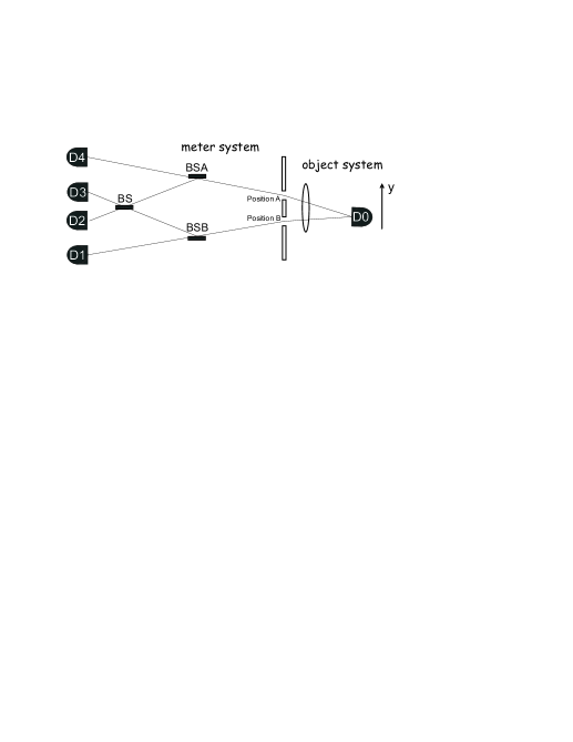
Figure 2: Sketched setup of a ‘partially active’ quantum eraser. An entangled photon pair can be produced either in region $A$ or in region $B$. If the detectors $D1$ or $D4$ click, one knows the production region $A$ or $B$, i.e. one has full which way information also for its photon partner. Clicks of the detectors $D2$ or $D3$ cannot contain this information which has been erased at the central beam splitter. Interference is observed only in this latter case. It is a ‘partially active’ eraser, because the mark is erased by a probabilistic law, however, the experimenter has still partially control over the erasure, he can choose the ratio of transmittivity to reflectivity of the beam splitter $BSA$ and $BSB$.

      (c) Passive eraser with “passive” measurements on the meter

Next we consider the setup in Fig. 3(c). We take advantage —and this is specific for kaons— of the passive measurement. Again the strangeness content of the object system —the kaon moving to the left hand side— is actively measured by inserting a piece of matter into the beam and thus scanning a given $t_{l}$ interval. In the beam of the meter no material piece is inserted and the kaon moving to the right propagates freely in space. This corresponds to a passive measurement of either strangeness or lifetime on the meter by recording the different decay modes of neutral kaons. If a semileptonic decay mode is found, the strangeness content is measured and the lifetime mark is erased. The distributions of the jointly detected events will show the characteristic interference fringes and antifringes. By contrast, if a $\pi\pi$ or a $\pi\pi\pi$ decay is observed, the lifetime is measured and thus “which width” information on the object system is obtained and no interference is seen in the joint events. Clearly we have a completely passive erasing operation on the meter, the experimenter has no control whether the lifetime mark is going to be read out or not.

This experiment is conceptually different from any other considered two–level quantum system.

      (d) Passive eraser with “passive” measurements

Fig. 3(d) sketches a setup where both kaons evolve freely in space and the experimenter observes passively their decay modes and times. The experimenter has no control over individual pairs neither on which of the two complementary observables is measured on each kaon, nor when it is measured.

This setup is totally symmetric, thus it is not clear which side plays the role of the meter. In this sense, one could claim that this experiment should not be considered as a quantum eraser. But one could also claim that this experiment reveals the true essence of the erasure phenomenon: Until the two measurements (one in each side) are completed, the factual situation is undefined; once one has the measurement results on both sides, the whole set of joint events can be classified in two subsets according to the kind of information (on strangeness or on lifetime) that has been obtained. The lifetime subset shows no interference, whereas fringes and antifringes appear when sorting the strangeness subset events according to the outcome, $K^{0}$ or $\bar{K}^{0}$, of the meter kaon.

Kaonic quantum erasers

(a) Active eraser with active measurements (S: active/active; T: active)

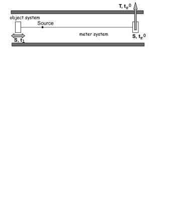
(b) Partially active eraser with active measurements (S: active/active; T: active)

(c) Passive eraser with passive measurements on the meter (S: active/passive; T: passive)

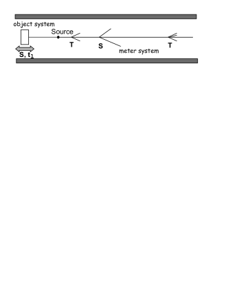
(d) Passive eraser with passive measurements (S: passive/passive; T: passive/passive)

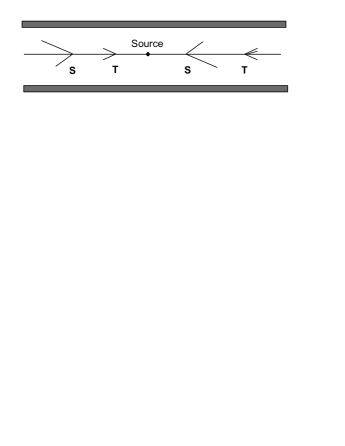
Figure 3: The figure shows four different setups for a quantum marking and quantum erasing experiment. The first three, (a), (b) and (c), have the object system on the left hand side on which the strangeness is always actively measured at time $t_{l}$. The setups (a) and (b) are analogous to existing quantum eraser experiments with entangled photons, see Fig. 1 and Fig. 2. The setup (c) has no analog, because only for kaons a passive measurement is possible. For the last setup, (d), it is not so clear which side plays the meter/object role as it is totally symmetric and it involves only passive measurements.

Summarizing, we have discussed four experimental setups combining active and passive measurement procedures which lead to the same observable probabilities. This is even true regardless of the temporal ordering of the measurements, as follows immediately from the fact that the $\Delta t$–dependent functions in eq.(17), eq.(18) and in eq.(19), which govern the shape of the interference pattern, are even in this variable $\Delta t=t_{l}-t_{r}$. Thus kaonic erasers can also be operated in the “delayed choice” mode as already described in Ref. [18]. In our view this adds further light to the very nature of the quantum eraser working principle: the way in which joint detected events are classified according to the available information. In the ‘delayed choice’ mode, a series of strangeness measurements is performed at different times $t_{l}$ on the object kaons and the corresponding outcomes are recorded. Later one can measure either lifetime or strangeness on the corresponding meter partner and, only now, full information allowing for a definite sorting of each pair is available. If we choose to perform strangeness measurements on the meter kaons and classify the joint events according the $K^{0}$ or $\bar{K}^{0}$ outcomes, we complete the information on each pair in such a way that oscillations and complementary anti–oscillations appear in the corresponding subsets. The alternative choice of lifetime measurements on meter kaons, instead, does not give the suitable information to classify the events in oscillatory subsets as before.

4 Conclusions

We have discussed the possibilities offered by neutral kaon states, such as those copiously produced by $\phi$–resonance decays at the DA$\Phi$NE machine, to investigate two fundamental issues of quantum mechanics: quantitative Bohr’s complementarity and quantum eraser phenomena. In both cases, the use of neutral kaons allows for a clear conceptual simplification and to obtain the relevant formulae in a transparent and non–controversial way.

A key point is that neutral kaon propagation through the $K_{S}$ and $K_{L}$ components automatically parallels most of the effects of double slit devices. Thanks to this, Bohr’s complementarity principle can be quantitatively discussed in the most simple and transparent way. Similarly, the relevant aspects of quantum marking and the quantum eraser admit a more clear treatment with neutral kaons than with other physical systems. This is particularly true when the eraser is operated in the ‘delayed choice’ mode and contributes to clarify the eraser’s working principle. Moreover, the possibility of performing passive measurements, a specific feature of neutral kaons not shared by other systems, has been shown to open new options for the quantum eraser. In short, we have seen that, once the appropriate neutral kaon states are provided as in the DA$\Phi$NE machine, most of the additional requirements to investigate fundamental aspects of quantum mechanics are automatically offered by Nature for free.

The CPLEAR experiment [19] did only part of the job (active strangeness–strangeness measurements), but the KLOE $2$ experiment could do the full program!

Acknowledgement: The authors thank the projects SGR–994, FIS2005–1369 and EURIDICE HPRN-CT-2002-00311. The latter allowed Beatrix Hiesmayr to work as a postdoc together with Albert Bramon and Gianni Garbarino in Barcelona, where the idea of the kaonic quantum eraser was born. We would also like to thank Antonio DiDomenico for inviting us to the very interesting Frascati–Workshop “Neutral kaon interferometry at a $\Phi$–Factory: from Quantum Mechanics to Quantum Gravity”.

References

- 1 . R.P. Feynman, R.B. Leighton and M. Sands, The Feynman Lectures on Physics, Vol. 3, (Addison-Wesley, 1965), p. 1-1, p. 11-20.
- 2 . D. Greenberger and A. Yasin, Phys. Lett. A 128, 391 (1988).
- 3 . B.-G. Englert, Phys. Rev. Lett. 77, 2154 (1996).
- 4 . A. Bramon, G. Garbarino and B. C. Hiesmayr, Phys. Rev. A 69, 022112 (2004).
- 5 . B.C. Hiesmayr and V. Vedral, “Interferometric wave-particle duality for thermodynamical systems”, quant-ph/0501015.
- 6 . M. Arndt, O. Nairz, J. Vos-Andreae, C. Keller, G. Van der Zouw and A. Zeilinger, Nature 401, 680682 (1999).
- 7 . M. O. Scully and K. Drhl, Phys. Rev. A 25, 2208 (1982).
- 8 . S. Drr and G. Rempe, Opt. Commun. 179, 323 (2000).
- 9 . T.J. Herzog, P.G. Kwiat, H. Weinfurter and A. Zeilinger, Phys. Rev. Lett 75, 3034 (1995).
- 10 . Y.-H. Kim, R. Yu, S.P. Kuklik, Y. Shih and M.O. Scully, Phys. Rev. Lett. 84, 1 (2000).
- 11 . R.A. Bertlmann and B.C. Hiesmayr, Phys. Rev. A 63, 062112 (2001.
- 12 . T. Tsegaye, G. Bjrk, M. Atatre, A.V. Sergienko, B.W.A. Saleh and M.C. Teich, Phys. Rev. A 62, 032106 (2000).
- 13 . S.P. Walborn, M.O. Terra Cunha, S. Padua and C.H. Monken, Phys. Rev. A 65, 033818 (2002).
- 14 . A. Trifonov, G. Bjrk, J. Sderholm and T. Tsegaye, Eur. Phys. J. D 18, 251 (2002).
- 15 . H. Kim, J. Ko and T. Kim, Phys. Rev. A 67, 054102 (2003).
- 16 . Y. Aharonov and M.S. Zubairy, Science 307, 875 (2005).
- 17 . A. Bramon, G. Garbarino and B. C. Hiesmayr, Phys. Rev. Lett. 92, 020405 (2004).
- 18 . A. Bramon, G. Garbarino and B. C. Hiesmayr, Phys. Rev. A 68, 062111 (2004).
- 19 . A. Apstolakis et.al., Phys. Lett. B 422, 339 (1998).