hep-ph/0609307

IFIC/06-31

Experimental tests for the Babu-Zee two–loop model of Majorana neutrino masses

D. Aristizabal Sierra and M. Hirsch

AHEP Group, Instituto de Física Corpuscular – C.S.I.C./Universitat de València
Edificio de Institutos de Paterna, Apartado 22085, E–46071 València, Spain.

The smallness of the observed neutrino masses might have a radiative origin. Here we revisit a specific two-loop model of neutrino mass, independently proposed by Babu and Zee. We point out that current constraints from neutrino data can be used to derive strict lower limits on the branching ratio of flavour changing charged lepton decays, such as $\mu\rightarrow e\gamma$. Non-observation of Br($\mu\rightarrow e\gamma$) at the level of $10^{-13}$ would rule out singly charged scalar masses smaller than 590 GeV (5.04 TeV) in case of normal (inverse) neutrino mass hierarchy. Conversely, decay branching ratios of the non-standard scalars of the model can be fixed by the measured neutrino angles (and mass scale). Thus, if the scalars of the model are light enough to be produced at the LHC or ILC, measuring their decay properties would serve as a direct test of the model as the origin of neutrino masses.

1 Introduction

During the past few years neutrino oscillation experiments have firmly established that neutrinos have non-zero masses and mixing angles among the different generations [1]. While for the absolute scale of neutrino mass only upper limits of the order $m_{\nu}\sim{\cal O}(2\hskip 2.84526pt{\rm eV})$ exist [2], two neutrino mass squared differences and two neutrino angles are by now known quite precisely [3]. These are the atmospheric neutrino mass, $\Delta m^{2}_{\rm Atm}=(2.0-3.2)$ [$10^{-3}$ eV²], and angle, $\sin^{2}\theta_{\rm Atm}=(0.34-0.68)$, as well as the solar neutrino mass $\Delta m^{2}_{\odot}=(7.1-8.9)$ [$10^{-5}$ eV²], and angle, $\sin^{2}\theta_{\odot}=(0.24-0.40)$, all numbers at 3 $\sigma$ c.l. For the remaining neutrino angle, the so-called Chooz [4] or reactor neutrino angle $\theta_{R}$, a global fit to all neutrino data [3] currently gives a limit of $\sin^{2}\theta_{R}\leq 0.04$ $@$ 3 $\sigma$ c.l.

From a theoretical perspective, there exist several options to explain the smallness of the observed neutrino masses. Perhaps the simplest - but certainly the most popular - possibility is the seesaw mechanism [5, 6]. Many variants of the seesaw exist, see for example the recent review [7]. However, most realizations of the seesaw make use of a large scale, typically the Grand Unification Scale, to suppress neutrino masses and are, therefore, only indirectly testable.

On the other hand, many neutrino mass models exist, in which the scale of lepton number violation can be as low as the electro-weak scale or lower. Examples are supersymmetric models with violation of R-parity [8, 9], models with Higgs triplets [10] or a combination of both [11], leptoquarks [12] or radiative models, both with neutrino masses at 1-loop [13, 14] or at 2-loop [12, 15, 16] order. Radiative mechanisms might be considered especially appealing, since they generate small neutrino masses automatically, essentially due to loop factors.

In this paper we will concentrate on a model of neutrino masses, proposed independently by Zee [15] and Babu [16], in which neutrino masses arise only at 2-loop order. The model introduces two new charged scalars, $h^{+}$ and $k^{++}$, both singlets under $SU(2)_{L}$, which couple only to leptons. One can easily estimate, see fig. (1) and the discussion in the next section, that neutrino masses in this setup are of order $m_{\nu}\sim(f^{2}h)/(16\pi^{2})^{2}(m_{\mu}^{2}/m_{S})$, i.e. ${\cal O}\sim 1$ eV for couplings $f$ and $h$ of order ${\cal O}(1)$ and scalar mass parameters, $m_{S}$, of order ${\cal O}(100)$ GeV. Given that current neutrino data requires at least one neutrino to have a mass of order ${\cal O}(0.05)$ eV, one expects that the new scalars should have masses in the range ${\cal O}(0.1-1)$ TeV. The model is therefore potentially testable at near-future accelerators, such as the LHC or ILC.

Figure 1: Feynman diagram for the 2-loop Majorana neutrino masses in the model of [15, 16].

Babu and Macesanu [17] recently re-analyzed this model in light of solar and atmospheric neutrino oscillation data. They identified the regions in parameter space, in which the model can explain the experimental neutrino data and tabulated in some detail constraints on the model parameters, which can be derived from the non-observation of various lepton flavour violating decay processes. Here, we extend upon the results presented in [17] by pointing out that (a) current neutrino data can be used to derive absolute lower limits on the branching ratios of the processes $l_{\alpha}\rightarrow l_{\beta}\gamma$. Especially important in view of future experimental sensitivities [18] is that $Br(\mu\rightarrow e\gamma)\geq 10^{-13}$ is guaranteed for charged scalar masses smaller than 590 GeV (5.04 TeV) in case of normal (inverse) neutrino mass hierarchy. And (b) decay branching ratios of the non-standard scalars of the model can be fixed by the measured neutrino angles (and mass scale). Thus, if the scalars of the model are light enough to be produced at the LHC or ILC, measuring their decay properties would serve as a direct test of the model as the origin of neutrino masses.

The rest of this paper is organized as follows. In the next section, we discuss the Lagrangian of the model, as well as its parameters in light of current oscillation data. In this part we will make extensive use of the results of [17]. In section 3, we calculate flavour violating charged lepton decays, $l_{a}\rightarrow l_{b}l_{c}l_{d}$ and $l_{\alpha}\rightarrow l_{\beta}\gamma$, discussing their connection with neutrino physics in some detail. Then, we consider the decays of the new scalars at future colliders, presenting ranges for various decay branching ratios as predicted by current neutrino data. We then close with a short discussion.

2 Neutrino masses at 2-loop

As mentioned above, the model we consider [15, 16] is a simple extension of the standard model, containing two new scalars, $h^{+}$ and $k^{++}$, both singlets under $SU(2)_{L}$. Their coupling to standard model leptons is given by

$${\cal L}=f_{\alpha\beta}(L^{Ti}_{\alpha L}CL^{j}_{\beta L})\epsilon_{ij}h^{+}+h^{\prime}_{\alpha\beta}(e^{T}_{\alpha R}Ce_{\beta R})k^{++}+{\rm h.c.}$$ (1)

Here, $L_{L}$ are the standard model (left-handed) lepton doublets, $e_{R}$ the charged lepton singlets, $\alpha,\beta$ are generation indices and $\epsilon_{ij}$ is the completely antisymmetric tensor. Note that $f$ is antisymmetric, while $h^{\prime}$ is symmetric. Assigning $L=2$ to $h^{-}$ and $k^{++}$, eq. (1) conserves lepton number. Lepton number violation in the model resides only in the following term in the scalar potential

$${\cal L}=-\mu h^{+}h^{+}k^{--}+{\rm h.c.}$$ (2)

Here, $\mu$ is a parameter with dimension of mass, its value is not predicted by the model. However, vacuum stability arguments can be used to derive an upper bound for this parameter [17]. For $m_{h}\sim m_{k}$ this bound reads

$$\mu\leq(6\pi^{2})^{1/4}m_{h}.$$ (3)

The setup of eq. (1) and eq. (2) generates Majorana neutrino masses via the two-loop diagram shown in fig. (1). The resulting neutrino mass matrix can be expressed as

$${\cal M}^{\nu}_{\alpha\beta}=\frac{8\mu}{(16\pi^{2})^{2}m_{h}^{2}}f_{\alpha x}\omega_{xy}f_{y\beta}{\cal I}(\frac{m_{k}^{2}}{m_{h}^{2}}),$$ (4)

with summation over $x,y$ implied. The parameters $\omega_{xy}$ are defined as $\omega_{xy}=m_{x}h_{xy}m_{y}$, with $m_{x}$ the mass of the charged lepton $l_{x}$. Following [17] we have rewritten $h_{\alpha\alpha}=h^{\prime}_{\alpha\alpha}$ and $h_{\alpha\beta}=2h^{\prime}_{\alpha\beta}$. ${\cal I}(r)$ finally is a dimensionless two-loop integral given by

$${\cal I}(r)=-\int_{0}^{1}dx\int_{0}^{1-x}dy\frac{1}{x+(r-1)y+y^{2}}\log\frac{y(1-y)}{x+ry}.$$ (5)

For non-zero values of $r$, ${\cal I}(r)$ can be solved only numerically. We note that for the range of interest, say $10^{-2}\leq r\leq 10^{2}$, ${\cal I}(r)$ varies quite smoothly between (roughly) $3\leq{\cal I}(r)\leq 0.2$.

Eq.(4) generates only two non-zero neutrino masses. This can easily be seen from its index structure: ${\rm Det}({\cal M}^{\nu})={\rm Det}(f_{\alpha x}\omega_{xy}f_{y\beta})={\rm Det}(f_{\alpha\beta})=0$. The model therefore can not generate a degenerate neutrino spectrum. One can find the eigenvector for the massless state, it is proportional to

$$v_{0}^{T}={\cal N}(1,-\epsilon,\epsilon^{\prime})$$ (6)

where ${\cal N}=(1+\epsilon^{2}+\epsilon^{\prime 2})^{-1/2}$ is a normalization factor. Here we have introduced

$$\epsilon=\frac{f_{e\tau}}{f_{\mu\tau}}, \epsilon^{\prime}=\frac{f_{e\mu}}{f_{\mu\tau}}.$$ (7)

With ${\cal M}^{\nu}.v_{0}=0$ one can express the parameters $\epsilon$ and $\epsilon^{\prime}$ also in terms of the entries of the neutrino mass matrix. A straightforward calculation yields

$$\epsilon = \frac{m_{12}m_{33}-m_{13}m_{23}}{m_{22}m_{33}-m_{23}^{2}},$$ (8)

$$\epsilon = \frac{m_{12}m_{23}-m_{13}m_{22}}{m_{22}m_{33}-m_{23}^{2}}.$$

Interestingly, eq. (8) can be rewritten directly as a function of the measured neutrino angles. For normal hierarchy, i.e. $m_{\nu_{1,2,3}}\simeq(0,m,M)$, one obtains

$$\epsilon = \tan\theta_{12}\frac{\cos\theta_{23}}{\cos\theta_{13}}+\tan\theta_{13}\sin\theta_{23}e^{-i\delta},$$ (9)

$$\epsilon^{\prime} = \tan\theta_{12}\frac{\sin\theta_{23}}{\cos\theta_{13}}-\tan\theta_{13}\cos\theta_{23}e^{-i\delta}.$$

Note, that eq. (9) does not depend on neutrino masses, and that current data on neutrino angles require both $\epsilon$ and $\epsilon^{\prime}$ to be non-zero. On the other hand, in the case of inverse hierarchy, $m_{\nu_{1,2,3}}\simeq(M,\pm M+m,0)$, eq. (8) leads to

$$\epsilon = -\cot\theta_{13}\sin\theta_{23}e^{-i\delta},$$ (10)

$$\epsilon^{\prime} = \cot\theta_{13}\cos\theta_{23}e^{-i\delta}.$$

Again, both $\epsilon$ and $\epsilon^{\prime}$ have to be different from zero. Note that $\delta$ in eq. (9) and (10) is a CP-violating phase, which reduces to a CP-sign $\delta=0,\pi$ in case of real parameters.

With the equations outlined above, we are now in a position to give an estimate of the typical size of neutrino masses in the model. For an analytical understanding, the following approximation is quite helpful. Since $m_{e}\ll m_{\mu},m_{\tau}$, $\omega_{ee}$, $\omega_{e\mu}$ and $\omega_{e\tau}$ are expected to be much smaller than the other $\omega_{\alpha\beta}$. Then, in the limit $\omega_{ee}=\omega_{e\mu}=\omega_{e\tau}=0$, eq. (4) reduces to

$${\cal M}^{\nu}=\zeta\left(\begin{array}[]{cccc}\epsilon^{2}\omega_{\tau\tau}+2\epsilon\epsilon^{\prime}\omega_{\mu\tau}+\epsilon^{\prime 2}\omega_{\mu\mu}&\epsilon\omega_{\tau\tau}+\epsilon^{\prime}\omega_{\mu\tau}&-\epsilon\omega_{\mu\tau}-\epsilon^{\prime}\omega_{\mu\mu}\cr&&\cr\cdot&\omega_{\tau\tau}&-\omega_{\mu\tau}\cr&&\cr\cdot&\cdot&\omega_{\mu\mu}\end{array}\right),$$ (11)

where

$$\zeta = \frac{8\mu}{(16\pi^{2})^{2}}\frac{f_{\mu\tau}^{2}}{m_{h}^{2}}{\cal I}(\frac{m_{k}^{2}}{m_{h}^{2}}).$$ (12)

From eq. (11) it is easy to estimate the typical ranges of parameters, for which the model can explain current neutrino data. In case of normal hierarchy, a large atmospheric angle requires $\omega_{\mu\mu}\simeq-\omega_{\mu\tau}\simeq\omega_{\tau\tau}$. Thus, we find the constraint

$$h_{\tau\tau}\simeq(\frac{m_{\mu}}{m_{\tau}})h_{\mu\tau}\simeq(\frac{m_{\mu}}{m_{\tau}})^{2}h_{\mu\mu}.$$ (13)

On the other hand, a solar angle of order $\tan\theta_{\odot}\simeq\frac{1}{\sqrt{2}}$ requires $\epsilon\sim\epsilon^{\prime}\simeq 1/2$, see eq. (9). Inverse hierarchy still requires $\omega_{\mu\mu}\simeq\omega_{\mu\tau}\simeq\omega_{\tau\tau}$, although with a different relative sign, while $\epsilon$ and $\epsilon^{\prime}$ have to be much larger, i.e. $\epsilon\sim\epsilon^{\prime}\simeq\frac{M}{m}$, see also eq. (10).

What is the maximal neutrino mass the model can generate? Using eqs (3) and (13), this upper limit can be estimated choosing $h_{\mu\mu}$ maximal. Motivated by perturbativity, we choose $h_{\mu\mu}=1$. Then, $m_{k}\raise 1.29167pt\hbox{$\;>$\kern-7.5pt\raise-4.73611pt\hbox{$\sim\;$}}800$ GeV is required (see the next section), and with $m_{h}=100$ GeV, ${\cal I}(r)\simeq 0.3$ results. Putting finally $f_{\mu\tau}=0.03$ we arrive at $m_{\nu_{3}}\simeq 0.05$ eV. Since all other parameters in this estimate have been put to extreme values, $f_{\mu\tau}\geq 0.03$ will be required in general. Obviously, even considering only neutrino data, the parameters of the model are already severely constrained.

3 Flavour violating charged lepton decays

Due to the flavour off-diagonal couplings of the $k^{++}$ and $h^{+}$ scalars to SM leptons, the model has sizeable non-standard flavour violating charged lepton decays. An extensive list of constraints on model parameters, derived from the observed upper limits of these decays, can be found in [17]. Here we will discuss decays of the type $l_{\alpha}\rightarrow l_{\beta}\gamma$ and their connection with neutrino physics. As the experimentally most interesting case we concentrate on $\mu\rightarrow e\gamma$. A short comment on $\tau$ decays is given at the end of this section.

Consider the partial decay width of $l_{\alpha}\rightarrow l_{\beta}\gamma$ induced by the $h^{+}$ scalar loop shown in fig. (2). In the limit of $m_{\beta}\ll m_{\alpha}$ it is given by

$$\Gamma(l_{\alpha}\rightarrow l_{\beta}\gamma)=2\alpha m_{\alpha}^{3}(\frac{m_{\alpha}}{96\pi^{2}})^{2}\Big{(}\frac{(f^{\dagger}f)_{\beta\alpha}}{m_{h}^{2}}\Big{)}^{2}.$$ (14)

We will be interested in deriving a lower bound on the numerical value of eq. (14) in the following. Note, that although there is a graph similar to the one shown in fig. (2) with a $k^{++}$ in the intermediate state, there is no interference between the two contributions (in the limit where the smaller lepton mass is put to zero). Thus, in deriving the lowest possible value of Br($\mu\rightarrow e\gamma$) we will put the contribution from $k^{++}$ to zero. Any finite contribution from the doubly charged scalars would lead to stronger bounds on $m_{h}$ than the numbers quoted below.

Using eqs (7), (11) and (12) we can rewrite eq. (14) as

$$Br(\mu\rightarrow e\gamma) = \frac{\alpha\epsilon^{2}m_{\mu}\pi^{3}}{18\sqrt{6}\Gamma_{\mu}h_{\mu\mu}^{2}{\cal I}(r)^{2}}\frac{m_{\nu}^{2}}{m_{h}^{2}}$$ (15)

$$\simeq 4.5\cdot 10^{-10}\Big{(}\frac{\epsilon^{2}}{h_{\mu\mu}^{2}{\cal I}(r)^{2}}\Big{)}\Big{(}\frac{m_{\nu}}{\rm 0.05\hskip 2.84526pteV}\Big{)}^{2}\Big{(}\frac{\rm 100\hskip 2.84526ptGeV}{m_{h}}\Big{)}^{2}$$ (16)

With $\epsilon$ non-zero, constrained by eq. (9) or eq. (10) in case of normal or inverse hierarchy, Br($\mu\rightarrow e\gamma$) has to be non-zero as well. Its smallest numerical value is found for the largest possible value of $h_{\mu\mu}$ and ${\cal I}(r)$.

Figure 2: Example diagrams for flavour changing charged lepton decays in the model. In addition to the diagrams shown, there are also box graphs involving $h^{+}$ contributing to $l_{a}\rightarrow l_{b}l_{c}l_{d}$, as well as graphs with $k^{++}$, similar to the one shown, contributing to $l_{a}\rightarrow l_{b}\gamma$.

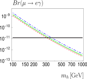
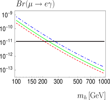
Figure 3: Conservative lower limit on the branching ratio Br($\mu\rightarrow e\gamma$) as a function of the charged scalar mass $m_{h}$ for normal hierarchy. The three lines are for the current solar angle $\sin^{2}\theta_{12}$ best fit value (full line) and 3 $\sigma$ lower (dashed line) and upper (dot-dashed line) bounds. To the left $\delta=0$, to the right $\delta=\pi$. Other parameters fixed at $\sin^{2}\theta_{23}=0.5$, $\sin^{2}\theta_{13}=0.040$ and $\Delta m^{2}_{\rm Atm}=2.0\cdot 10^{-3}$ eV².

In order to calculate ${\cal I}(r)$ we need to fix $r$ consistent with all experimental constraints. This is done in the following way. The decay width $l_{a}\rightarrow l_{b}l_{c}l_{d}$ induced by virtual exchange of $k^{++}$, see fig. (2), is, in the limit $m_{b},m_{c},m_{d}\ll m_{a}$,

$$\Gamma(l_{a}\rightarrow l_{b}l_{c}l_{d})=\frac{1}{8}\frac{m_{a}^{5}}{192\pi^{3}}\Big{|}\frac{h_{ab}h_{cd}^{*}}{m_{k}^{2}}\Big{|}^{2}.$$ (17)

The most relevant constraint for the current discussion is derived from the upper bound on $\tau\rightarrow 3\mu$ decay, which yields,

$$\frac{|h_{\mu\tau}h_{\mu\mu}|}{m_{k}^{2}}\raise 1.29167pt\hbox{$\;<$\kern-7.5pt\raise-4.73611pt\hbox{$\sim\;$}}10^{-7}\hskip 5.69054pt{\rm GeV}^{-2}.$$ (18)

For $h_{\mu\tau}(\frac{m_{\tau}}{m_{\mu}})=h_{\mu\mu}=1$, this bound implies $m_{k}\raise 1.29167pt\hbox{$\;>$\kern-7.5pt\raise-4.73611pt\hbox{$\sim\;$}}770$ GeV. For any fixed value of $h_{\mu\mu}$, we can therefore fix the minimum value of $r$, i.e. the maximum allowed value of ${\cal I}(r)$, which in turn fixes the lower bound on Br($\mu\rightarrow e\gamma$).

Fig. (3) shows the resulting lower limit on Br($\mu\rightarrow e\gamma$) as a function of the charged scalar mass $m_{h}$ for the case of normal hierarchy. In this plot, we have assumed that the parameters $\mu$, $h_{\mu\mu}$ (and $\Delta m^{2}_{\rm Atm}$) take their maximal (minimal) allowed values, thus we consider this limit conservative. We would like to stress again, that any non-zero contributions to the decay $\mu\rightarrow e\gamma$ from $k^{++}$ can only increase Br($\mu\rightarrow e\gamma$).

Fig. (4) and (5) show the dependence of the limit on Br($\mu\rightarrow e\gamma$) on the three neutrino angles. Both plots are for the case of normal hierarchy. Larger values of $\theta_{12}$ ($\theta_{23}$) result in larger (smaller) upper bounds. Smaller ranges of these parameters obviously lead to tighter predictions. For $\theta_{13}$, below approximately $\sin^{2}\theta_{13}\raise 1.29167pt\hbox{$\;<$\kern-7.5pt\raise-4.73611pt\hbox{$\sim\;$}}0.01$ the dependence of Br($\mu\rightarrow e\gamma$) is rather weak.

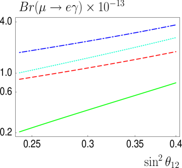
Figure 4: Dependence of the lower limit on Br$(\mu\rightarrow e\gamma)$ for normal hierarchy on neutrino angles, for $h_{\mu\mu}=1,\delta=\pi,m_{h}=10^{3}\mbox{GeV}$. Left plot: ($\sin^{2}\theta_{23}=0.68$, $\sin^{2}\theta_{13}=0$) dashed line, ($\sin^{2}\theta_{23}=0.68$, $\sin^{2}\theta_{13}=0.040$) full line, ($\sin^{2}\theta_{23}=0.34$, $\sin^{2}\theta_{13}=0$) dash-dotted line, ($\sin^{2}\theta_{23}=0.34$, $\sin^{2}\theta_{13}=0.040$) dotted line. Right plot: ($\sin^{2}\theta_{12}=0.40$, $\sin^{2}\theta_{13}=0$) dash-dotted line, ($\sin^{2}\theta_{12}=0.40$, $\sin^{2}\theta_{13}=0.040$) dotted line, ($\sin^{2}\theta_{12}=0.24$, $\sin^{2}\theta_{13}=0$) dashed line, ($\sin^{2}\theta_{12}=0.24$, $\sin^{2}\theta_{13}=0.040$) full line.

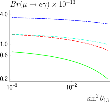
Figure 5: Dependence of the lower limit on Br$(\mu\rightarrow e\gamma)$ for normal hierarchy on the reactor angle, for $h_{\mu\mu}=1,\delta=\pi,m_{h}=10^{3}\mbox{GeV}$. Other parameters are chosen as ($\sin^{2}\theta_{23}=0.68$, $\sin^{2}\theta_{12}=0.40$) dashed line, ($\sin^{2}\theta_{23}=0.68$, $\sin^{2}\theta_{12}=0.24$) full line, ($\sin^{2}\theta_{23}=0.34$, $\sin^{2}\theta_{12}=0.40$) dash-dotted line and ($\sin^{2}\theta_{23}=0.34$, $\sin^{2}\theta_{12}=0.24$) dotted line.

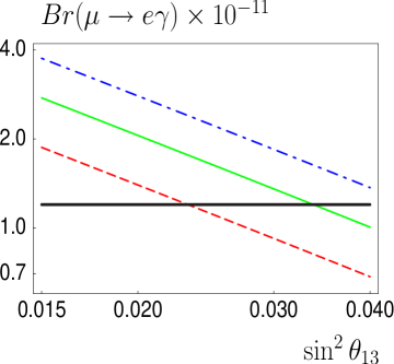
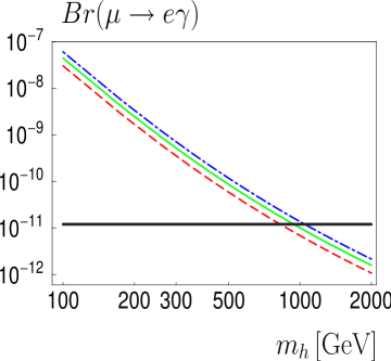
Figure 6: Lower limit on Br($\mu\rightarrow e\gamma$) for inverted hierarchy, to the left: versus the reactor angle; to the right: versus $m_{h}$. Parameter choices as before. The three lines are for the current $\sin^{2}\theta_{23}$ best fit value (full line) and 3 $\sigma$ upper (dot-dashed line) and lower (dashed line) bounds.

Fig. (6) shows the calculated lower limit on Br($\mu\rightarrow e\gamma$) for the case of inverted hierarchy, both, versus the reactor angle and versus $m_{h}$. Due to the fact that $\epsilon$ must be larger than $\epsilon\simeq\sin\theta_{23}/\tan\theta_{13}$, the expected values for Br($\mu\rightarrow e\gamma$) turn out to be much bigger than for the case of normal hierarchy. Even Br($\mu\rightarrow e\gamma$) $\raise 1.29167pt\hbox{$\;<$\kern-7.5pt\raise-4.73611pt\hbox{$\sim\;$}}10^{-11}$ requires already TeV-ish masses for $m_{h}$.

The most conservative limits for $m_{h}$ are always found for $\delta=\pi$, $\sin^{2}\theta_{12}=(\sin^{2}\theta_{\odot})^{Min}$, $\sin^{2}\theta_{23}=(\sin^{2}\theta_{\rm Atm})^{Max}$ and $\sin^{2}\theta_{13}=(\sin^{2}\theta_{\rm R})^{Max}$. For the current bound of $Br(\mu\to e\gamma)\leq 1.2\times 10^{-11}$, we find $m_{h}\geq 160\,\mbox{GeV}$ ($m_{h}=825\,\mbox{GeV}$) for normal (inverse) hierarchy. Future experiments [18] expect to lower this limit to $Br(\mu\to e\gamma)\leq 10^{-13}$, resulting in $m_{h}\geq 590\,\mbox{GeV}$ ($m_{h}=5040\,\mbox{GeV}$). Given these numbers, one expects that the MEG experiment [18] will see the first evidence for $\mu\rightarrow e\gamma$ in the near future, if the model discussed here indeed is the origin of neutrino masses.

Finally, we would like to mention that the decays $\tau\rightarrow\mu\gamma$ and $\tau\rightarrow e\gamma$ can be constrained in a similar way. However, the resulting lower limits, also of order ${\cal O}(10^{-13})$, are far below the near-future experimental sensitivities and thus less interesting.

4 Accelerator tests of the model

In this section we will briefly discuss some possible accelerator signals of the model. With the couplings of $h^{+}$ and $k^{++}$ tightly constrained by neutrino physics and flavour violating lepton decays, it turns out that various decay branching ratios can be predicted. Observing the corresponding final states could serve as a definite test of the model as the origin of neutrino masses.

In [17] it has been estimated that at the LHC discovery of $k^{++}$ might be possible up to masses of $m_{k}\leq 1$ TeV approximately. In the following we will therefore always assume that $m_{k}\leq 1$ TeV and, in addition, $m_{h}\leq 0.5$ TeV. Given the discussion of the previous section, this range of masses implies that $\mu\rightarrow e\gamma$ should be seen at the MEG experiment.

The $h^{+}$ will decay to leptons with a partial decay width of, in the limit $m_{\alpha}=0$,

$$\Gamma(h^{+}\rightarrow l_{\alpha}\sum_{\beta}{\nu_{\beta}})=\frac{m_{h}}{16\pi}\sum_{\beta}f_{\alpha\beta}^{2}.$$ (19)

We can re-express eq. (19) in terms of the parameters $\epsilon$ and $\epsilon^{\prime}$ as

$$Br(h^{+}\rightarrow e\sum_{\beta}{\nu_{\beta}})=\frac{\epsilon^{2}+\epsilon^{\prime 2}}{2(1+\epsilon^{2}+\epsilon^{\prime 2})},$$ (20)

$$Br(h^{+}\rightarrow\mu\sum_{\beta}{\nu_{\beta}})=\frac{1+\epsilon^{\prime 2}}{2(1+\epsilon^{2}+\epsilon^{\prime 2})},$$

$$Br(h^{+}\rightarrow\tau\sum_{\beta}{\nu_{\beta}})=\frac{1+\epsilon^{2}}{2(1+\epsilon^{2}+\epsilon^{\prime 2})}.$$

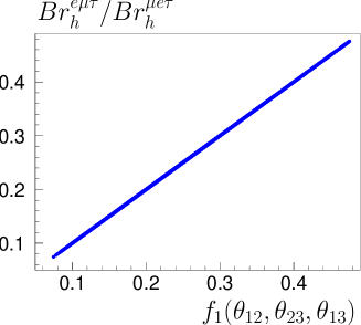
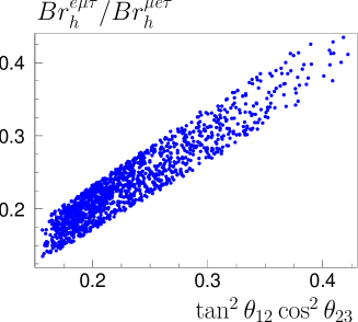
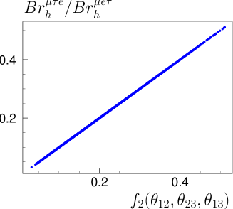
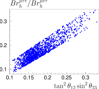
Figure 7: Ratios of decay branching ratios $Br_{h}^{ijk}$, see text, versus $f_{1}(\theta_{12},\theta_{23},\theta_{13})=\tan\theta_{12}\frac{\cos\theta_{23}}{\cos\theta_{13}}+\tan\theta_{13}\sin\theta_{23}$ (top); and $f_{2}(\theta_{12},\theta_{23},\theta_{13})=\tan\theta_{12}\frac{\sin\theta_{23}}{\cos\theta_{13}}-\tan\theta_{13}\cos\theta_{23}$ (bottom). In the right plots $\sin^{2}\theta_{13}<2.5\times 10^{-3}$ has been assumed. All points satisfy updated experimental neutrino data.

It is therefore possible to directly “measure” $\epsilon^{2}$ or $\epsilon^{\prime 2}$ by calculating ratios of branching ratio differences, such as the ones shown in fig. (7). Here,

$$Br_{h}^{ijk}\equiv Br(h^{-}\to\nu\ell_{i}^{-})-Br(h^{-}\to\nu\ell_{j}^{-})+Br(h^{-}\to\nu\ell_{k}^{-}).$$ (21)

The plots on the left in fig. (7) show calculated ratios of branching ratios versus eq. (9), i.e. normal hierarchy, versus $\epsilon$ (top) and $\epsilon^{\prime}$ (bottom). All points are obtained by numerically diagonalizing eq. (4) for random parameters and checking for consistency with all experimental constraints. However, since $\theta_{13}$ is unkown, eq. (9) can be numerically calculated, but at the moment not experimentally determined. Thus, the plots on the right of the figure show the same ratios of branching ratios, but versus $(\tan\theta_{12}\cos\theta_{12})^{2}$ and $(\tan\theta_{12}\sin\theta_{12})^{2}$. The cut on $\sin^{2}\theta_{13}$ of $\sin^{2}\theta_{13}<2.5\times 10^{-3}$ in this plot is motivated by the expected sensitivity of the next generation of reactor experiments [19, 20]. The width of the band of points in these plots indicates the uncertainty with which the corresponding ratios can be predicted.

In case of normal (inverse) hierarchy, assuming best fit parameters for the neutrino angles, eq. (20) indicates that the branching ratios for $e,\mu$ and $\tau$ final states of $h^{+}$ decays should scale as $2/12:5/12:5/12$ ($1/2:1/4:1/4$). Inserting the current 3 $\sigma$ ranges of the angles, following eqs. (9) and (10) results in the following predicted ranges

$$Br(h^{+}\rightarrow e\sum_{\beta}{\nu_{\beta}})=[0.13,0.22]\hskip 14.22636pt([0.48,0.50])$$ (22)

$$Br(h^{+}\rightarrow\mu\sum_{\beta}{\nu_{\beta}})=[0.31,0.50]\hskip 14.22636pt([0.17,0.34])$$

$$Br(h^{+}\rightarrow\tau\sum_{\beta}{\nu_{\beta}})=[0.31.0.50]\hskip 14.22636pt([0.18,0.35])$$

for normal (inverse) hierarchy. The different predicted branching ratios for final states with electrons should make it nearly straightforward to distinguish normal and inverse hierarchy. Measuring any branching ratio outside the range given in eq. (22) would rule out the model as possible origin of neutrino masses.

The doubly charged scalar of the model decays either to two same-sign leptons or to two $h^{+}$ final states. The partial width to leptons is, for $m_{\alpha},m_{\beta}=0$,

$$\Gamma(k^{++}\rightarrow l_{\alpha}l_{\beta})=\frac{m_{k}}{16\pi}h_{\alpha\beta}^{2}$$ (23)

whereas the decay width to two $h^{+}$ can be calculated to be

$$\Gamma(k^{++}\rightarrow h^{+}h^{+})=\frac{1}{16\pi}\frac{\mu^{2}}{m_{k}}\beta(\frac{m_{h}^{2}}{m_{k}^{2}})$$ (24)

Here, $\beta(x^{2})=\sqrt{1-4x^{2}}$ is a kinematical factor.

The couplings $h_{\alpha\beta}$ in eq.(23) are constrained by neutrino physics, see eq.(13), and by lepton flavour violating decays of the type $l_{a}\rightarrow l_{b}l_{c}l_{d}$. For $m_{k}\leq 1$ TeV the couplings $h_{ee}$, $h_{e\mu}$ and $h_{e\tau}$ are constrained to be smaller than $0.4$, $4\cdot 10^{-3}$ and $7\cdot 10^{-2}$ [17]. Thus, the leptonic final states of $k^{++}$ decays are mainly like-sign muon pairs (and possibly electrons).

An interesting situation arises, if $m_{k}\geq 2m_{h}$. In this case, one can measure the lepton number violating parameter $\mu$ of eq.(2) by measuring the branching ratio of $k^{++}\rightarrow h^{+}h^{+}$. Combining eq. (23) and eq. (24) we can write

$$Br(k^{++}\rightarrow h^{+}h^{+})\simeq\frac{\mu^{2}\beta}{m_{k}^{2}h_{\mu\mu}^{2}+\mu^{2}\beta}\simeq\frac{fm_{h}^{2}\beta}{m_{k}^{2}h_{\mu\mu}^{2}+fm_{h}^{2}\beta}.$$ (25)

Here, $h_{ee}\ll h_{\mu\mu}$ has been assumed. (For non-zero $h_{ee}$ replace simply $h_{\mu\mu}\rightarrow h_{\mu\mu}+h_{ee}$ in eq. (25).) Plots of constant Br$(k^{++}\rightarrow h^{+}h^{+})$ in the plane ($m_{k},m_{h}$) are shown in fig. (8). Here, $\mu=fm_{h}$, with $f=(6\pi^{2})^{1/4}$ has been used.

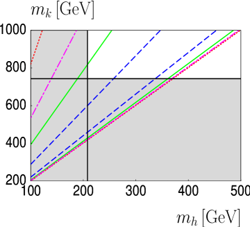
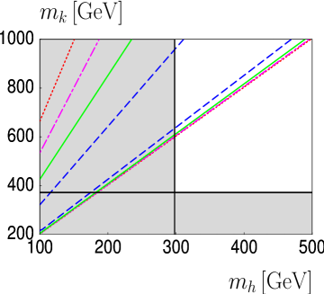
Figure 8: Lines of constant Br$(k^{++}\rightarrow h^{+}h^{+})$, assuming to the left $h_{\mu\mu}=1$: $Br^{hh}_{k}=0.1,0.2,0.3$ and $0.4$ for dotted, dash-dotted, full and dashed line. The vertical line corresponds to $m_{h}=208\,\mbox{GeV}$ for which $Br(\mu\to e\gamma)=1.2\times 10^{-11}$ and horizontal line to $m_{k}=743\,\mbox{GeV}$ for which $Br(\tau\to 3\mu)=1.9\times 10^{-6}$, i.e. parameter combinations to the left/below this line are forbidden. Plot on the right assumes $h_{\mu\mu}=0.5$. Lines are for $Br^{hh}_{k}=0.4,0.5,0.6$ and $0.7$, dotted, dash-dotted, full and dashed line. Again the shaded regions are excluded by Br$(\mu\to e\gamma)$ and Br$(\tau\to 3\mu)$.

Fig. (8) shows the resulting branching ratios for 2 values of $h_{\mu\mu}$, fixing in both cases the couplings $f_{\alpha\beta}$ such that the atmospheric neutrino mass is correctly reproduced. For $h_{\mu\mu}\raise 1.29167pt\hbox{$\;<$\kern-7.5pt\raise-4.73611pt\hbox{$\sim\;$}}0.2$ the current limit on Br$(\mu\to e\gamma)$ rules out all $m_{h}\raise 1.29167pt\hbox{$\;<$\kern-7.5pt\raise-4.73611pt\hbox{$\sim\;$}}0.5$ TeV, thus this measurement is possible only for $h_{\mu\mu}\raise 1.29167pt\hbox{$\;>$\kern-7.5pt\raise-4.73611pt\hbox{$\sim\;$}}0.2$. Note that smaller values of $\mu$ lead to smaller neutrino masses, thus upper bounds on the branching ratio for $Br^{hh}_{k}$ can be interpreted as upper limit on the neutrino mass in this model.

5 Conclusion

The observed smallness of neutrino masses could be understood if it has a radiative origin. In this paper, we have studied some phenomenological aspects of one well-known incarnation of this idea [15, 16], in which neutrino masses arise only at 2-loop order.

Given the observed neutrino masses and angles, it turns out that the parameters of this model are very tightly constrained already today and thus it is possible to make various predictions for the near future. Perhaps the phenomenologically most important one is, that one expects that the process $\mu\rightarrow e\gamma$ has to be observed in the next round of experiments, i.e. Br($\mu\rightarrow e\gamma$) $\geq 10^{-13}$ is guaranteed for singly charged scalar masses smaller than 590 GeV (5.04 TeV) for normal (inverse) hierarchical neutrino masses, and larger or even much larger branching ratios are expected in general. At least for the case of inverse hierarchy an upper limit on the decay $\mu\rightarrow e\gamma$ of this order would certainly remove most of the motivation to study this model.

On the other hand, if $\mu\rightarrow e\gamma$ is observed in the near future, it will be interesting to search for the charged scalars of the model at the LHC. As we have shown, in this case, several branching ratios of the decays of both, the singly and the doubly charged scalar are tightly fixed, mainly by data on neutrino angles. Observation of branching ratios outside the ranges discussed, would then definitely rule out the model as a possible explanation of neutrino masses.

References

[1]
Y. Fukuda et al. [Super-Kamiokande Collaboration],
Phys. Rev. Lett. 81, 1562 (1998)
[arXiv:hep-ex/9807003];
Q. R. Ahmad et al. [SNO Collaboration],
Phys. Rev. Lett. 89, 011301 (2002)
[arXiv:nucl-ex/0204008];
K. Eguchi et al. [KamLAND Collaboration],
Phys. Rev. Lett. 90, 021802 (2003)
[arXiv:hep-ex/0212021].
[2]
S. Eidelman et al. [Particle Data Group],
Phys. Lett. B 592, 1 (2004).
[3]
M. Maltoni, T. Schwetz, M. A. Tortola and J. W. F. Valle,
New J. Phys. 6 (2004) 122
[arXiv:hep-ph/0405172]. (V5) in the archive provides updated numbers
taking into account all relevant data as of June 2006.
[4]
M. Apollonio et al.,
Eur. Phys. J. C 27 (2003) 331
[arXiv:hep-ex/0301017].
[5]
P. Minkowski,
Phys. Lett. B 67 (1977) 421.
[6]
M Gell-Mann, P Ramond, R. Slansky, in Supergravity, ed. P. van
Niewenhuizen and D. Freedman (North Holland, 1979);
T. Yanagida, in KEK lectures, ed. O. Sawada and A. Sugamoto,
KEK, 1979
[7]
J. W. F. Valle,
arXiv:hep-ph/0608101.
[8]
L. J. Hall and M. Suzuki,
Nucl. Phys. B231, 419 (1984).
[9]
M. Hirsch et al.,
Phys. Rev. D62, 113008 (2000), [hep-ph/0004115],
Err-ibid. D65:119901,2002;
ibid D68, 013009 (2003)
[Erratum-ibid. D 71, 059904 (2005)]
[10]
J. Schechter and J. W. F. Valle,
Phys. Rev. D 22, 2227 (1980).
[11]
D. Aristizabal Sierra, M. Hirsch, J. W. F. Valle and A. Villanova del Moral,
Phys. Rev. D 68, 033006 (2003)
[arXiv:hep-ph/0304141].
[12]
J. F. Nieves,
Nucl. Phys. B 189, 182 (1981).
[13]
A. Zee,
Phys. Lett. B 93 (1980) 389
[Erratum-ibid. B 95 (1980) 461].
[14]