Long distance effects in semi-inclusive B decays

Abstract

We discuss some issues on factorization of long distance effects for semi-inclusive $B$ decay spectra in full QCD and in the effective theory.

1 Introduction

Let us consider B meson decays into a QCD jet plus non QCD partons, such as a real photon or a lepton pair. This decay is characterized by three fundamental mass scales, the heavy flavor mass $m_{b}$ and the energy $E_{X}$ and invariant mass of the jet $m_{X}$. The threshold region is defined as the region where $m_{X}\ll E_{X}$, that is the region where the final observed state has large energy and the emission of real soft and collinear partons is inhibited. Close to threshold, in the perturbative calculation, the partial cancellation of infrared real and virtual contributions produces large logarithms in the ratio of $m_{X}$ and the hard scale $Q$. In the heavy quark effective theory (HQET), the heavy quark is replaced by a static color charge, leaving unchanged infrared exchanges in the heavy meson, and therefore the structure of the large infrared logarithms. By integrating out the heavy flavor mass in HQET, the only remaining scales in the hadronic subprocess are $m_{X}$ and $E_{X}$ and the hard scale $Q$ is identified with $E_{X}$. Infrared large logarithms at threshold occur in the ratio $E_{X}/m_{X}$ [2, 3]. Such logarithms have to be resummed in order not to spoil the perturbative expansion. We will elaborate on some issues related to the universality of long distance effects.

2 Universality of QCD form factor

For the semileptonic decay $B\rightarrow X_{u}l\nu$, the most general differential distribution can be written in a factorized form:

$$\frac{1}{\Gamma}\frac{d^{3}\Gamma}{dxdudw} = C\left[x,w;\alpha(w\,m_{b})\right]\,\sigma\left[u;\alpha(w\,m_{b})\right]\,+$$ (1)

$$+ \,d\left[x,u,w;\alpha(w\,m_{b})\right]~{},$$

where

$$w\,=\,\frac{2E_{X}}{m_{b}},\qquad x\,=\,\frac{2E_{l}}{m_{b}}$$ (2)

and

$$u\,=\,\frac{E_{X}-\sqrt{E_{X}^{2}-m_{X}^{2}}}{E_{X}+\sqrt{E_{X}^{2}-m_{X}^{2}}}\,\approx\,\frac{m_{X}^{2}}{4\,E_{X}^{2}}.$$ (3)

The distribution is normalized to the radiatively-corrected total semileptonic width $\Gamma$. We have two short-distance, process-dependent functions, the coefficient function $C\left[x,w;\alpha(w\,m_{b})\right]$ and the remainder function $d\left[x,u,w;\alpha(w\,m_{b})\right]$. All the infrared logarithms are resummed into a universal, long-distance dominated, QCD form factor $\sigma\left[u;\alpha(w\,m_{b})\right]$. The running coupling constant is set to the hard scale of the system, $Q$, where $Q\,=\,w\,m_{b}\,=\,2E_{X}$.

In the radiative decay $B\rightarrow X_{s}\,\gamma$, a similar formula holds for the single differential spectrum in the hadronic mass

$$\frac{1}{\Gamma_{R}}\frac{d\Gamma_{R}}{dt_{s}}\, = \,C_{R}\left[\alpha(m_{b})\right]\,\sigma\left[t_{s};\,\alpha(m_{b})\right]\,+$$ (4)

$$+ \,d_{R}\left[t_{s};\,\alpha(m_{b})\right],$$

where $t_{s}\,=\,m_{X_{s}}^{2}/m_{b}^{2}$. The form factor $\sigma$, being the universal form factor, is the same appearing in formula (1), while the coefficient and the remainder function, dependent on the process, are different. In the radiative decay, $w\sim 1$, allowing the replacement $\alpha(w\,m_{b})\,\rightarrow\,\alpha(m_{b})$; the distribution (4) contains a constant coupling $\alpha(m_{b})\simeq 0.22$. Due to kinematics, such replacement cannot be done in the semileptonic differential distribution (1). The important issue is that the form factor $\sigma$, although being universal, depends on one kinematical variable $m_{X_{s}}^{2}/m_{b}^{2}$ in the radiative case, while it depends on two kinematical variables, $u$ and $w$, in the semileptonic case. Such difference leads to a natural division into two classes for the double and single differential distributions, obtained integrating the general triple differential distribution (1) [3, 4, 5]. The first class contains distributions not integrated over the energy $E_{X}$, f.i. the single distribution in $E_{X}$: they have the same form factor as radiative decays. The second class contains distributions integrated over the energy $E_{X}$, f.i. the single distribution in $m_{X}$ or in $E_{l}$: their dependence on the universal form factor has been spoiled by the integration, and they have the same form factor as radiative decays only at leading logarithmic order. Since soft logarithms signal long distance effects, there is a different long distance structure with respect to distributions in the first class and to radiative decay, due to the integration over the hard scale. In other terms, while in radiative decays the form factor $\sigma$ is fixed at a hard scale $Q=m_{b}$, in the second class the form factor is integrated on $Q$ with a generic weight function $\phi(Q)$, dependent on kinematics, from low values up to $m_{b}$.

3 Semileptonic spectra

Let us consider, f.i., the hadron energy spectrum, $d\,\Gamma/d\,E_{X}$, belonging to the first class mentioned before. As well known, its shape presents the so called Sudakov shoulder, related to the occurrence of infrared singularities close to the threshold $E_{X}=m_{b}/2$. At lowest fixed order $O(\alpha)$, the parton process $b\rightarrow u\,l\,\nu\,g$, where $g$ is a real gluon, contributes to the decay. Above the threshold, at $E_{X}=E_{u}+E_{g}\geq m_{b}/2$, large infrared logarithms, of the form $\log(E_{X}-m_{b}/2)$, appear and become singular at $E_{X}\rightarrow m_{b}/2^{+}$. Virtual contributions cannot cancel such singularity, since in the virtual process $b\rightarrow u\,l\,\nu$ the energy of the up quark, $E_{u}=E_{X}$, cannot exceed the energy $m_{b}/2$. The solution is to abandon the fixed order calculation and resum into a form factor all large infrared logarithms. Resummation completely eliminates the singularity, leaving only an effect in the characteristic Sudakov shoulder.

The single differential distribution in $E_{X}$ is obtained by integrating (1). Let us use the adimensional variables defined in (2) and (3). Since there are large logarithms only for $w>1$, we are interested in the resummed formula in that region only. We have [3]:

$$\frac{1}{\Gamma}\frac{d\Gamma}{dw} = C_{1}\left(\alpha\right)\Big{\{}1-C_{2}\left(\alpha\right)\,\mathchar 28934\relax\left[w-1;\,\alpha(m_{b})\right]\Big{\}}$$ (5)

$$+ R(w;\,\alpha),$$

where $C_{1}\left(\alpha\right)$ and $C_{2}\left(\alpha\right)$ are two coefficient functions, and $R(w;\,\alpha)$ is a remainder function, vanishing at $w=1$. They have a perturbative expansion in $\alpha$, whose coefficients are constant in the case of the coefficients, depend on $w$ for the remainder. The form factor $\mathchar 28934\relax$ is the partially integrated or cumulative form factor $\mathchar 28934\relax(u,\alpha)$, defined as:

$$\mathchar 28934\relax(u;\,\alpha)\,=\,\int_{0}^{u}du^{\prime}\,\sigma(u^{\prime};\,\alpha).$$ (6)

It resums all infrared logarithms, and it is universal, being the same as in the radiative decay; at any order in perturbation theory the hadron energy semileptonic spectra and the radiative one have the same infrared logarithms. The form factor $\mathchar 28934\relax(u;\,\alpha)$ has an exponential form:

$$\qquad\mathchar 28934\relax\,=\,e^{G},$$ (7)

with

$$G(u;\alpha)\, = \,\sum_{n=1}^{\infty}\sum_{k=1}^{n+1}G_{nk}\,\alpha^{n}\,L^{k},$$

$$L\, \equiv \,\log\frac{1}{u}.$$ (8)

The situation changes radically if we take a differential spectrum belonging to the second class defined above, f.i. the single differential semileptonic spectrum in the hadronic mass or the distribution in the light–cone momentum, normalized to $m_{b}$, $p_{+}=(E_{X}-|\vec{p}_{X}|)/m_{b}$. After integration, such distributions can be rearranged in a factorized form, with the requirement that the form factor contains all the infrared logarithms; however, the logarithmic tower will be different with respect to the radiative decay [4, 5].

F.i., in the distribution $1/\Gamma\,d\Gamma/d{p}_{+}$, we can construct a cumulative form factor $\mathchar 28934\relax_{P}(p_{+};\,\alpha)$ in analogy with (6). The related form factor can also be exponentiated:

$$\mathchar 28934\relax_{P}\,=\,e^{G_{P}}$$ (9)

with

$$G_{P}\left(p_{+};\,\alpha\right)\, = \,\sum_{n=1}^{\infty}\sum_{k=1}^{n+1}G_{Pnk}\,\alpha^{n}\,L_{P}^{k},$$

$$L_{P}\, \equiv \,\log\frac{1}{p_{+}}.$$ (10)

The difference in soft logarithms explicitly shows up when we compare the numerical coefficients $G_{nk}$ and $G_{Pnk}$:

$${G}_{P12} = G_{12},$$

$${G}_{P11} = G_{11}+0.18,$$

$${G}_{P23} = G_{23},$$

$${G}_{P22} = G_{22}+0.089-0.0046\,n_{f},$$

and so on; $n_{f}$ is the number of active flavors.

4 Soft and collinear emissions

The QCD form factor $\mathchar 28934\relax$ can be written as a convolution of two functions, each of them corresponding to distinct sources of large corrections: the shape function $f$, resumming infrared logarithms due to soft contributions, and a coefficient or jet function $J$. The shape function has the characteristics of a quark distribution function and it is well defined in HQET. Upon introducing a factorization scale $\mu_{F}$ we can write

$$\mathchar 28934\relax[u;\,\alpha(Q)]=J(u;Q,\mu_{F})\;\otimes\;f(u;\mu_{F}).$$ (11)

The coefficient function resums all hard collinear logarithms, as well as soft effects between the factorization scale $\mu_{F}$ and the hard scale of QCD. The factorization scale $\mu_{F}$ can be identified with the ultraviolet cut off of the shape function in the HQET. The physical basis of such factorization is that soft logarithms are related to longer distance effects with respect to hard collinear logarithms. In the radiative case $Q=m_{b}$, and it is a natural choice setting $\mu_{F}=m_{b}$ as well:

$$\mathchar 28934\relax(m_{b})=J(m_{b})\;\;f(m_{b}).$$ (12)

In the semileptonic case, that is not always the case. At the end of section (2) we have represented schematically the construction of single and double differential decay spectra as an integration in the hard scale $Q$ weighted by a generic function $\phi(Q)$, dependent on kinematics. That simplification is helpful here as well. Let us write

$$\int_{0}^{m_{b}}dQ\,\phi(Q)\;\sigma(Q)=$$ (13)

$$= \int_{0}^{m_{b}}dQ\,\phi(Q)\;J(Q,\mu_{F})\;f(\mu_{F}).$$

In order to avoid substantial soft effects in the jet factor, one has to take $\mu_{F}$ of order $Q$. Since Q is integrated over, also $\mu_{F}$ has to be changed and one has to know the shape function as a function of $\mu_{F}$. This is to be contrasted with the radiative case, in which it is sufficient to know the shape function at the single point $\mu_{F}=m_{b}$. Let us stress that it is essential to factorize all the soft logarithms in the shape function. One can then replace the perturbatively evaluation of the shape function with a non perturbative one (f.i. lattice QCD), including also non perturbative soft effects, such as Fermi motion of the $b$ quark inside the $B$ meson.

5 Long distance effects

Quite often, non perturbative long distance effects are included in a phenomenological way by convoluting the perturbatively calculated spectrum with a non perturbative structure function. Being non perturbative, the latter is generally not computed, but, f.i., parameterized and fitted to the experimental spectrum in the radiative decay and then used into the theoretical prediction for the semileptonic decay. This procedure is not without risks, since, as seen before, the correlation between different decays is not always immediate, even at the perturbative level. It introduces the dominant source of uncertainty in the CKM determination of $V_{ub}$ from the semileptonic decay.

Another possibility is to include such effects without convoluting the perturbative spectrum with a non perturbative structure function, thus remaining within the perturbation theory framework. Effects due to the motion of the $b$ quark inside the meson will be taken into account modifying the QCD running coupling constant into an effective coupling according to a model [6]. The effective coupling will also help solving regularization problems present already in the perturbation theory, that are traditionally cured by means of arbitrary prescriptions. They are due to the fact that resummation formulas do not exclude very low energy kinematical regions, where the running coupling constant hits the Landau pole. The effective coupling is built in two steps [6]. First, a dispersion relation is used to analytically extend the running coupling constant $\alpha$ to a coupling $\bar{\alpha}$ without the Landau pole; $\bar{\alpha}$ has the same physical discontinuities than $\alpha$ and the same high energy behavior, but it has a finite limit at zero momentum transfer. The second step consists of resumming in the effective coupling $\tilde{\alpha}$ the secondary emissions off the radiated gluons. The resummation formula is the standard one, but it is controlled by the discontinuity of $\bar{\alpha}$, instead than $\alpha$:

$$\tilde{\alpha}(k_{\perp}^{2})\,=\,\frac{i}{2\pi}\,\int_{0}^{k_{\perp}^{2}}\,ds\,{\rm Disc}_{s}\,\frac{\bar{\alpha}(-s)}{s}.$$ (14)

The effective coupling has an expansion in powers of $\alpha$ and its usage can be considered a change of scheme. As in the previous sections, we can factorize the decay spectra and calculate the universal form factor $\sigma$. The difference is that now in the perturbative calculation the effective coupling is used. Factorization is easily performed in the Mellin space:

$$\sigma_{N}(\alpha)\,=\,\int_{0}^{1}\,(1-u)^{N-1}\,\sigma(u;\,\alpha)\,du.$$ (15)

The form factor has an exponential form in $N$-space:

$$\sigma_{N}(\alpha)\,=\,e^{G_{N}(\alpha)},$$ (16)

where the exponent of the form factor reads:

$$G_{N}(\alpha)\,=\,\int_{0}^{1}\frac{dy}{y}\left[(1-y)^{N-1}-1\right]$$

$$\left\{\int_{Q^{2}y^{2}}^{Q^{2}y}\frac{dk_{\perp}^{2}}{k_{\perp}^{2}}\tilde{A}\left[\tilde{\alpha}(k_{\perp}^{2})\right]\,+\,\tilde{B}\left[\tilde{\alpha}(Q^{2}y)\right]\right.$$

$$\left.+\,\tilde{D}\left[\tilde{\alpha}(Q^{2}y^{2})\right]\right\}.$$ (17)

This formula is the same as the standard resummation formula, where effective couplings and functions have replaced the standard ones. The functions $\tilde{A}(\tilde{\alpha}),\,\tilde{B}(\tilde{\alpha})$ and $\tilde{D}(\tilde{\alpha})$ have expansions in powers of the effective coupling, and are obtained by matching order for order in $\alpha$ the standard formula with (5).

The form factor in momentum space is obtained by inverse transform:

$$\sigma(t;\,\alpha)\,=\,\int_{C-i\infty}^{C+i\infty}\frac{dN}{2\pi i}(1-t)^{-N}\,\sigma_{N}(\alpha),$$ (18)

where the constant $C$ is chosen so that the integration contour in the $N$-plane lies to the right of all the singularities of $\sigma_{N}(\alpha)$. As anticipated, no prescription is needed because $\sigma_{N}(\alpha)$ is analytic for ${\rm Re}\,N\,>\,0$.

6 Comparison with data

In Fig. 1 the invariant hadron mass distribution for the radiative decay, $d\Gamma_{r}/dm_{X}$ is compared with experimental data from the BaBar collaboration [7]. The theoretical curve, calculated in the model described in the previous section [6], shows a good agreement with data. The model has no free parameters; however, one can choose to best fit the theoretical curve to data by using as free parameter $\alpha(m_{Z})$, and obtain $\alpha_{S}(m_{Z})\,=\,0.123\,\pm\,0.003$. Let us observe that the data with $m_{X}<1.1$ GeV are not representative; they show the $K^{\star}$ peak, which cannot be reproduced in this approach.

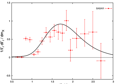
Figure 1: Comparison between theory and Babar data for the $B\rightarrow X_{s}\gamma$ invariant hadron mass distribution at $\alpha(m_{Z})\,=\,0.123$.

Another good agreement is obtained by comparing the photon energy spectrum with data from the Cleo Collaboration [8], as shown in Fig. 2. In the $B$ rest-frame, $t\,=\,m_{X}^{2}/m_{B}^{2}\,=\,1\,-\,2E_{\gamma}/m_{B}$. The photon energies are however measured in the $\mathchar 28935\relax(4S)$ rest frame, in which the $B$ mesons have a small, non-relativistic motion. In order to model the Doppler effect, it is possible to convolute the theoretical curve for $E_{\gamma}$ — computed with a $B$ meson at rest — with a normal distribution of $\sigma_{\gamma}\,=\,100$ or $150$ MeV.

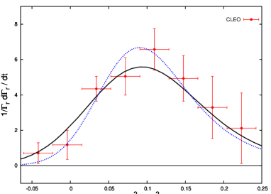
Figure 2: Comparison between theory and Cleo data for $B\rightarrow X_{s}\gamma$ photon spectrum. Dotted line (blue): $\alpha_{S}(m_{Z})\,=\,0.118$ and $\sigma_{\gamma}\,=\,100$ MeV to model the Doppler effect (see text); continuous line (black): $\alpha_{S}(m_{Z})\,=\,0.117$ and $\sigma_{\gamma}\,=\,150$ MeV.

Among semileptonic decays, let us consider the invariant hadron mass distribution, as shown in Fig. 3, in comparison with data from the BaBar collaboration [9]. Points with $m_{X}\,<\,400$ MeV, which are dominated by the $\pi$ peak, are discarded, as well as points with $m_{X}\,>\,2.6$ GeV, which give basically no information on the signal. Once again, there is a good agreement between theory and data.

The only distribution where the agreement with data is less satisfying is the electron spectrum in semi-leptonic decays, as shown in Fig. 4, where data from Belle collaboration have been used [10]. Theory predicts a harder spectrum, with a broad maximum around $2.1$ GeV, while data peak at lower energies. More accurate data, and possibly perturbative calculations in the complete NNLO approximation, are needed to clarify such discrepancy.

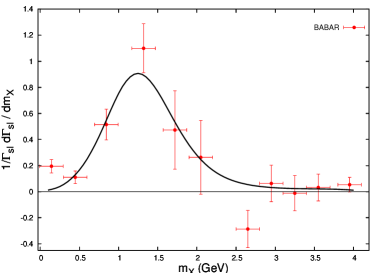
Figure 3: Comparison between theory and Babar data for invariant hadron mass distribution in semileptonic decays for $\alpha_{S}(m_{Z})\,=\,0.119$.

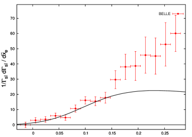
Figure 4: Comparison between theory and Belle data for the electron spectrum in semileptonic decay for $\alpha_{S}(m_{Z})\,=\,0.135$. The data and the theory are normalized to one in the charm background free region $0\,<\,\bar{x}_{e}\,<\,0.125$.

References

- [1]
- [2] U. Aglietti, Nucl. Phys. B 610, 293 (2001) [arXiv:hep-ph/0104020].
- [3] U. Aglietti, G. Ricciardi and G. Ferrera, Phys. Rev. D 74 (2006) 034004 [arXiv:hep-ph/0507285]
- [4] U. Aglietti, G. Ricciardi and G. Ferrera, Phys. Rev. D 74 (2006) 034005 [arXiv:hep-ph/0509095].
- [5] U. Aglietti, G. Ricciardi and G. Ferrera, Phys. Rev. D 74 (2006) 034006 [arXiv:hep-ph/0509271].
- [6] U. Aglietti, G. Ferrera and G. Ricciardi, [arXiv:hep-ph/0608047].
- [7] B. Aubert et al. [BABAR Collaboration], Phys. Rev. D 72 (2005) 052004 [arXiv:hep-ex/0508004].
- [8] S. Chen et al. [CLEO Collaboration], Phys. Rev. Lett. 87 (2001) 251807 [arXiv:hep-ex/0108032].
- [9] B. Aubert et al. [BABAR Collaboration], Phys. Rev. Lett. 96 (2006) 221801 [arXiv:hep-ex/0601046].
- [10] A. Limosani et al. [Belle Collaboration], Phys. Lett. B 621 (2005) 28 [arXiv:hep-ex/0504046].