Three body kinematic endpoints in SUSY models with non-universal Higgs masses

Abstract:

We derive and present expressions for the kinematic endpoints that arise in the invariant mass distributions of visible decay products of cascade decays featuring a two body decay followed by a three body decay. This is an extension of a current technique that addresses chains of successive two body decays. We then apply these to a supergravity model with Non-Universal Higgs Masses (NUHM), having simulated a data set using the ATLFAST detector simulation. We find that, should such a model be chosen by nature, the endpoints will be visible in ATLAS data, and we discuss the problems associated with mass reconstruction in models with a similar phenomenology.

1 Introduction

The Standard Model (SM) of particle physics has been enormously successful in predicting a wide range of phenomena with great accuracy and precision. In spite of this, however, there are specific issues that lead one to conclude that the SM is only an effective theory, which is thus incapable of describing physics at arbitrarily high energies. Searches for new physics in the ATLAS detector of the Large Hadron Collider (LHC) will be as exciting as they are challenging.

There is a plethora of models on the market that attempt to solve the problems of the SM, and supersymmetry is a relatively strong contender (see [1] for a concise introduction). By generalising the space-time symmetries of the gauge field theories of the SM to include a transformation between fermion and boson states, one introduces ‘superpartners’ for the SM particles which differ from their SM counterparts only by their spin if supersymmetry is unbroken; in the broken case they differ also in mass. In the process, one obtains a solution to the gauge hierarchy problem of the SM whilst also ensuring gauge unification at high energy scales, provided that the masses of the superpartners are below the TeV range. This provides the major motivation for supersymmetry searches at the LHC, and much effort has already been invested in developing strategies to measure particle masses and SUSY parameters at ATLAS.

It is noted that an interesting feature of most supersymmetric models is the existence of a multiplicatively conserved quantum number called R-parity, in which each superpartner is assigned $R=-1$, and each SM particle is assigned $R=+1$. R-parity conservation both ensures that sparticles must be produced in pairs and forces the lightest supersymmetric particle (LSP) to be absolutely stable. Thus, we obtain a ideal dark matter candidate, and can use recent measurements of dark matter relic density to impose constraints on SUSY models.

The lack of any current collider observations of sparticles means that SUSY must be a broken symmetry, and our ignorance of the breaking mechanism unfortunately means that the parameter set of the full Minimal Supersymmetric Standard Model (MSSM) numbers 124 (where SUSY breaking has given us 105 parameters on top of the SM). The difficulty of exploring such a large parameter space has meant that practically all phenomenological studies to date have been performed in simplified models in which various assumptions are made to reduce the parameter set to something of the order of 5, of which two are fixed. A popular example is the minimal Supergravity breaking scenario (mSUGRA), in which one unifies various GUT scale parameters, obtaining the following parameter set: the scalar mass $m_{0}$, the gaugino mass $m_{1/2}$, the trilinear coupling $A_{0}$, the ratio of Higgs expectation values tan$\beta$, and the sign of the SUSY Higgs mass parameter $\mu$.

Many ATLAS studies have been performed in the mSUGRA framework, using both full and fast simulation [2, 3, 4, 5, 6, 7, 8, 9], and one obtains an interesting range of phenomenologies over the parameter set. However, although one can devise relatively strong theoretical motivations for gaugino mass universality at the GUT scale, there is no reason why the soft supersymmetry-breaking scalar masses of the electroweak Higgs multiplets should be universal, and it is thus particularly important to consider models in which one breaks the degeneracy of these masses. These Non-Universal Higgs Mass (NUHM) models lead to yet more interesting phenomenological effects, and a set of benchmark points consistent with current measurements of the dark matter relic density, the $b\rightarrow s\gamma$ decay branching ratio and $g_{\mu}-2$ was presented in [10]. Furthermore, it was observed in [11] that relatively rare phenomena in the mSUGRA parameter space become much more ‘mainstream’ in NUHM models, and hence they make important cases for study, given that they are not excluded experimentally.

Our recent work has involved the use of Markov Chain methods to generalise the parameter spaces one can constrain using ATLAS data [6]. In the process, we have found that NUHM models are an interesting testing ground for new effects, and the purpose of this note is to highlight a particular observation related to cascade decays. For our particular model choice, decays featuring chains of successive two body decays are not present, and yet it is possible to observe decay chains involving a combination of two and three body decays. Thus, it should still be possible to measure masses by the standard method of searching for kinematic endpoints, but we will first need to derive expressions for their expected position. We note that this introduces an extra layer of ambiguity, since most previous studies have implicitly assumed that endpoints are due to two-body decay chains. Cascade decays featuring the three body decay mode could also occur in, for example, mSUGRA models, though to the best of our knowledge they have not been studied before.

Section 2 summarises our particular choice of NUHM model, reviewing both the mass spectrum and the relevant decay channels. We derive the three body endpoint positions for a general decay in section 3, before going on to apply these to our NUHM model in section 4. Finally, section 5 discusses the prospects for more detailed analysis of the NUHM model, before section 6 gives our final conclusions.

2 Selection of NUHM model

The NUHM parameter space is related to that of mSUGRA by the addition of two extra parameters that express the non-universality of the two MSSM Higgs doublets. These can be specified at the GUT scale as the masses $m_{H_{u}}^{2}$ and $m_{H_{d}}^{2}$, or alternatively the conditions of electroweak symmetry breaking allow one to trade these for the weak scale parameters $\mu$ and $m_{A}$. In selecting a model for study, we found the benchmark model $\gamma$ in [10] to be particularly interesting. The two body decay modes of the $\chi_{2}^{0}$ are not allowed, and hence one will not observe the characteristic two body endpoints seen in a variety of mSUGRA parameter space but, rather, will have to develop other strategies for analysis. Furthermore, it is compatible with all current experimental constraints arising from, e.g. WMAP and limits on the branching ratios of rare decays.

Figure 1: This cascade decay chain, including a three body decay, will give rise to kinematic endpoints.

Figure 2: The same decay as in figure 1, with the two leptons treated as a single object $L$.

The $\gamma$ benchmark point is specified as follows:

$m_{0}=328$ GeV, $m_{1/2}=247$ GeV

$tan\beta=20$, $A_{0}=0$, $|\mu|=325$ GeV and $m_{A}=240$ GeV

with a top quark mass of 178 GeV, and $\mu$ greater than zero.

We have used ISAJET 7.72 [12] to generate the mass spectrum and decay information for the point, and we summarise the results in tables 2, and tables 2 and 3 respectively. In addition, we used HERWIG 6.5 [13] to estimate a total SUSY production cross-section of 33 pb at this point. This differs from that given in reference [10], though is consistent with the fact that Herwig calculation is only performed to leading order, whereas [10] quotes a next to leading order result.

Particle	Mass/GeV
$\tilde{\chi}_{1}^{0}$	95
$\tilde{\chi}_{2}^{0}$	179
$\tilde{\chi}_{3}^{0}$	332
$\tilde{\chi}_{4}^{0}$	353
$\tilde{\chi}_{1}^{\pm}$	179
$\tilde{\chi}_{2}^{\pm}$	353
$\tilde{e}_{L}$	377
$\tilde{e}_{R}$	329
$\tilde{\nu_{e}}$	368
$\tilde{\tau}_{1}$	315
$\tilde{\tau}_{2}$	378
$\tilde{\nu_{\tau}}$	365
$\tilde{g}$	615
$\tilde{u}_{L}$	631
$\tilde{u}_{R}$	624
$\tilde{d}_{L}$	636
$\tilde{d}_{R}$	617
$\tilde{b}_{1}$	560
$\tilde{b}_{2}$	604
$\tilde{t}_{1}$	455
$\tilde{t}_{2}$	614
$h^{0}$	116
$H^{0}$	242
$A^{0}$	240
$H^{\pm}$	255

Table 1: The mass spectrum of the NUHM point defined in the text, as given by ISAJET 7.72 .

Decay Mode	BR
$\tilde{\chi}_{2}^{0}\rightarrow\tilde{\chi}_{1}^{0}q\bar{q}$	62%
$\tilde{\chi}_{2}^{0}\rightarrow\tilde{\chi}_{1}^{0}b\bar{b}$	19%
$\tilde{\chi}_{2}^{0}\rightarrow\tilde{\chi}_{1}^{0}l^{+}l^{-}$	3.5%
$\tilde{\chi}_{2}^{0}\rightarrow\tilde{\chi}_{1}^{0}\tau^{+}\tau^{-}$	2.7%
$\tilde{\chi}_{2}^{0}\rightarrow\tilde{\chi}_{1}^{0}\nu_{l}\bar{\nu_{l}}$	7.9%
$\tilde{\chi}_{2}^{0}\rightarrow\tilde{\chi}_{1}^{0}\nu_{\tau}\bar{\nu_{\tau}}$	3.9%
$\tilde{\chi}_{3}^{0}\rightarrow\tilde{\chi}_{1}^{\pm}W$	62%
$\tilde{\chi}_{3}^{0}\rightarrow\tilde{\chi}_{1}^{0}Z$	14%
$\tilde{\chi}_{3}^{0}\rightarrow\tilde{\chi}_{2}^{0}Z$	21%
$\tilde{\chi}_{3}^{0}\rightarrow\tilde{\chi}_{1}^{0}h$	2.7%
$\tilde{\chi}_{4}^{0}\rightarrow\tilde{\chi}_{1}^{\pm}W$	67%
$\tilde{\chi}_{4}^{0}\rightarrow\tilde{\chi}_{1}^{0}Z$	3.4%
$\tilde{\chi}_{4}^{0}\rightarrow\tilde{\chi}_{2}^{0}Z$	2.7%
$\tilde{\chi}_{4}^{0}\rightarrow\tilde{\chi}_{1}^{0}h$	9.1%
$\tilde{\chi}_{4}^{0}\rightarrow\tilde{\chi}_{1}^{0}H$	1.2%
$\tilde{\chi}_{4}^{0}\rightarrow\tilde{\chi}_{2}^{0}h$	16.5%
$\tilde{\chi}_{1}^{\pm}\rightarrow\tilde{\chi}_{1}^{0}W^{\pm}$	99%
$\tilde{\chi}_{2}^{\pm}\rightarrow\tilde{\chi}_{1}^{0}W^{\pm}$	9.7%
$\tilde{\chi}_{2}^{\pm}\rightarrow\tilde{\chi}_{2}^{0}W^{\pm}$	39%
$\tilde{\chi}_{2}^{\pm}\rightarrow\tilde{\chi}_{1}^{\pm}Z$	30%
$\tilde{\chi}_{2}^{\pm}\rightarrow\tilde{\chi}_{1}^{\pm}h$	20%

Table 2: The dominant chargino and neutralino decay processes at the NUHM point defined in the text, as given by ISAJET 7.72 , where $q$ denotes a quark from the first two generations, and $l$ is a lepton from the first two generations.

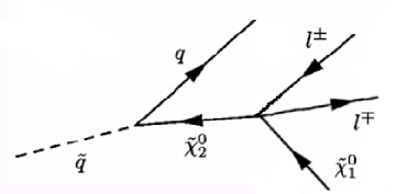
The most relevant part of the decay table concerns the decay modes of the $\tilde{\chi}^{0}_{2}$, and we see in table 2 that we do not obtain two body decays to sleptons, but rather have three body decays to quarks or leptons. Given that we have appreciable branching fractions for squark decays featuring $\tilde{\chi}^{0}_{2}$’s we will obtain decay chains of the form shown in figure 2, and thus we should be able to observe kinematic endpoints in lepton-jet invariant mass distributions using a similar method to that which has been previously documented for chains of successive two body decays. Each maximum will occur at a position given by a function of the three sparticle masses in the decay chain. Note that although the branching ratio for the decay $\tilde{\chi}_{2}^{0}\rightarrow\tilde{\chi}_{1}^{0}l^{+}l^{-}$ is small, the large SUSY production cross-section will guarantee a reasonable sample of events (approximately 3000 events for an initial ATLAS sample of $30\mbox{ fb}^{-1}$).

Decay Mode	BR	Decay Mode	BR	Decay Mode	BR
$(\tilde{u}_{L},\tilde{c}_{L})\rightarrow\tilde{\chi}^{0}_{2}q$	30%	$(\tilde{u}_{R},\tilde{c}_{R})\rightarrow\tilde{\chi}^{0}_{1}q$	96%	$\tilde{g}\rightarrow\tilde{b}_{1}b$	81%
$(\tilde{u}_{L},\tilde{c}_{L})\rightarrow\tilde{\chi}^{0}_{4}q$	2%	$(\tilde{u}_{R},\tilde{c}_{R})\rightarrow\tilde{\chi}^{0}_{2}q$	1%	$\tilde{g}\rightarrow\tilde{b}_{2}b$	4%
$(\tilde{u}_{L},\tilde{c}_{L})\rightarrow\tilde{g}q$	1.5%	$(\tilde{u}_{R},\tilde{c}_{R})\rightarrow\tilde{g}q$	2.3%	$\tilde{g}\rightarrow\tilde{\chi}_{1}^{\pm}q\bar{q}$	6.8%
$(\tilde{u}_{L},\tilde{c}_{L})\rightarrow\tilde{\chi}^{+}_{1}q$	63%			$\tilde{g}\rightarrow\tilde{\chi}_{1}^{0}q\bar{q}$	2.2%
$(\tilde{u}_{L},\tilde{c}_{L})\rightarrow\tilde{\chi}^{+}_{2}q$	2.5%			$\tilde{g}\rightarrow\tilde{\chi}_{2}^{0}q\bar{q}$	3.4%
$(\tilde{d}_{L},\tilde{s}_{L})\rightarrow\tilde{\chi}^{0}_{1}q$	2.1%	$(\tilde{d}_{R},\tilde{s}_{R})\rightarrow\tilde{\chi}^{0}_{1}q$	98%
$(\tilde{d}_{L},\tilde{s}_{L})\rightarrow\tilde{\chi}^{0}_{2}q$	30%	$(\tilde{d}_{R},\tilde{s}_{R})\rightarrow\tilde{\chi}^{0}_{2}q$	1%
$(\tilde{d}_{L},\tilde{s}_{L})\rightarrow\tilde{\chi}^{0}_{4}q$	2.7%
$(\tilde{d}_{L},\tilde{s}_{L})\rightarrow\tilde{\chi}^{-}_{1}q$	56%
$(\tilde{d}_{L},\tilde{s}_{L})\rightarrow\tilde{\chi}^{-}_{2}q$	8%
$\tilde{b}_{1}\rightarrow\tilde{\chi}_{1}^{0}b$	3.6%	$\tilde{t}_{1}\rightarrow\tilde{\chi}_{1}^{0}t$	17%
$\tilde{b}_{1}\rightarrow\tilde{\chi}_{2}^{0}b$	26%	$\tilde{t}_{1}\rightarrow\tilde{\chi}_{2}^{0}t$	13%
$\tilde{b}_{1}\rightarrow\tilde{\chi}_{3}^{0}b$	2.2%	$\tilde{t}_{1}\rightarrow\tilde{\chi}_{1}^{+}b$	50%
$\tilde{b}_{1}\rightarrow\tilde{\chi}_{4}^{0}b$	2.3%	$\tilde{t}_{1}\rightarrow\tilde{\chi}_{2}^{+}b$	20%
$\tilde{b}_{1}\rightarrow\tilde{\chi}_{1}^{-}t$	36%
$\tilde{b}_{1}\rightarrow\tilde{\chi}_{2}^{-}t$	26%
$\tilde{b}_{1}\rightarrow\tilde{t}_{1}W$	3.8%	$\tilde{t}_{2}\rightarrow\tilde{t}_{1}h$	3.6%
$\tilde{b}_{2}\rightarrow\tilde{\chi}_{1}^{0}b$	13%	$\tilde{t}_{2}\rightarrow\tilde{\chi}_{1}^{0}t$	1.8%
$\tilde{b}_{2}\rightarrow\tilde{\chi}_{2}^{0}b$	2.4%	$\tilde{t}_{2}\rightarrow\tilde{\chi}_{2}^{0}t$	8.5%
$\tilde{b}_{2}\rightarrow\tilde{\chi}_{3}^{0}b$	13%	$\tilde{t}_{2}\rightarrow\tilde{\chi}_{3}^{0}t$	9.5%
$\tilde{b}_{2}\rightarrow\tilde{\chi}_{4}^{0}b$	14%	$\tilde{t}_{2}\rightarrow\tilde{\chi}_{4}^{0}t$	27%
$\tilde{b}_{2}\rightarrow\tilde{\chi}_{1}^{-}t$	3.2%	$\tilde{t}_{2}\rightarrow\tilde{\chi}_{1}^{+}b$	22%
$\tilde{b}_{2}\rightarrow\tilde{\chi}_{2}^{-}t$	46%	$\tilde{t}_{2}\rightarrow\tilde{\chi}_{2}^{+}b$	21%
$\tilde{b}_{2}\rightarrow\tilde{t}_{1}W$	8.2%	$\tilde{t}_{2}\rightarrow\tilde{t}_{1}Z$	7%
$\tilde{l}_{L}\rightarrow\tilde{\chi}_{1}^{0}l$	12%	$\tilde{l}_{R}\rightarrow\tilde{\chi}_{1}^{0}l$	99%	$\tilde{\nu}_{l}\rightarrow\tilde{\chi}_{1}^{0}\nu_{l}$	17%
$\tilde{l}_{L}\rightarrow\tilde{\chi}_{2}^{0}l$	33%			$\tilde{\nu}_{l}\rightarrow\tilde{\chi}_{2}^{0}\nu_{l}$	24%
$\tilde{l}_{L}\rightarrow\tilde{\chi}_{1}^{-}\nu_{e}$	54%			$\tilde{\nu}_{l}\rightarrow\tilde{\chi}_{1}^{+}l$	59%
$\tilde{\tau}_{1}\rightarrow\tilde{\chi}_{1}^{0}\tau$	81%	$\tilde{\tau}_{2}\rightarrow\tilde{\chi}_{1}^{0}\tau$	16%	$\tilde{\nu}_{\tau}\rightarrow\tilde{\chi}_{1}^{0}\nu_{\tau}$	17%
$\tilde{\tau}_{1}\rightarrow\tilde{\chi}_{2}^{0}\tau$	6.9%	$\tilde{\tau}_{2}\rightarrow\tilde{\chi}_{2}^{0}\tau$	32%	$\tilde{\nu}_{\tau}\rightarrow\tilde{\chi}_{2}^{0}\nu_{\tau}$	24%
$\tilde{\tau}_{1}\rightarrow\tilde{\chi}_{1}^{-}\nu_{\tau}$	12%	$\tilde{\tau}_{2}\rightarrow\tilde{\chi}_{1}^{-}\nu_{\tau}$	50%	$\tilde{\nu}_{\tau}\rightarrow\tilde{\chi}_{1}^{+}\tau$	60%

Table 3: The dominant sfermion decay processes at the NUHM point defined in the text, as given by ISAJET 7.72 , where $q$ denotes a quark from the first two generations, and $l$ is a lepton from the first two generations.

3 Kinematic endpoint derivation

3.1 Introduction

The R-parity conservation referred to in section 1 has important implications for collider experiments: sparticles must be pair produced, and the LSP is stable. Thus, if R-parity is indeed conserved, each SUSY event at the LHC will have two sparticle decay chains, and the escaping LSPs will make it difficult to fully reconstruct events. It is, however, possible to construct distributions that are sensitive to sparticle masses.

In this paper we consider the decay $\tilde{q}\to q\tilde{\chi}_{2}^{0}$ followed by $\tilde{\chi}_{2}^{0}\to l^{+}l^{-}\tilde{\chi}_{1}^{0}$ as shown in figure 2. Such decays are fairly easy to select given that one can look for events with opposite-sign-same-flavour (OSSF) leptons, combined with the missing energy from the undetected neutralinos. By taking different combinations of the visible decay products, one can form various invariant masses; $m_{ll}$, $m_{llq}$, $m_{lq}^{high}$ and $m_{lq}^{low}$, where $m_{lq}^{high}$ is the higher of the two $m_{lq}$ invariant masses that can be formed in the event, and $m_{lq}^{low}$ is the lower. These will have maxima resulting from kinematic limits, whose position is given by a function of $m_{\tilde{q}}$, $m_{\tilde{\chi}_{2}^{0}}$ and $m_{\tilde{\chi}_{1}^{0}}$, and we derive these for each case below.

In the following derivations, we will use bold type for three momenta, and will denote four vector quantities by explicitly showing Lorentz indices. In addition, we will introduce a convention for representing squared masses by a non-bold character (e.g. $c=m_{\tilde{q}}^{2}$).

3.2 $m_{ll}$ endpoint

The endpoint of the $m_{ll}$ distribution results from the three body decay of the $\tilde{\chi}_{2}^{0}$, and is given trivially by the mass difference between the $\tilde{\chi}_{2}^{0}$ and the $\tilde{\chi}_{1}^{0}$:

$$(m_{ll}^{2})^{\mbox{\tiny max}}=(m_{\tilde{\chi}^{0}_{2}}-m_{\tilde{\chi}^{0}_{1}})^{2}.$$ (1)

3.3 $m_{llq}$ endpoint and threshold

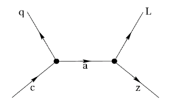
In calculating the $m_{llq}$ endpoint, we follow the method given in appendix E of [4] and treat the decay as shown in figure 2, where we have combined the two leptons into a single object $L$, with an invariant mass given by $m_{ll}$. We know from the dilepton invariant mass that $m_{ll}\equiv m_{L}$ must lie within a specific range:

$$m_{L}=\lambda(m_{a}-m_{z}),\lambda\in[0,1]$$ (2)

If we look at the decay of figure 2 in the rest frame of $a$, we can conserve four momentum to obtain the following expressions for the three momenta of $q$ and $L$:

$$\textbf{L}^{2}=\textbf{z}^{2}=[m_{L}^{2},m_{a}^{2},m_{z}^{2}]$$ (3)

$$\textbf{q}^{2}=\textbf{c}^{2}=[0,m_{a}^{2},m_{c}^{2}]$$ (4)

where

$$[x,y,z]\equiv\frac{x^{2}+y^{2}+z^{2}-2(xy+xz+yz)}{4y}$$ (5)

and we have treated the quark as massless.

Taking $q$ to be massless, the invariant mass of $q$ and $L$ is in general given by

$$m_{qL}^{2} = g_{\mu\nu}(L^{\mu}+q^{\mu})(L^{\nu}+q^{\nu})$$ (6)

$$= m_{L}^{2}+2|\textbf{q}|(E_{L}-|\textbf{L}|\cos\theta)$$ (7)

in which $\theta$ is the angle between $L$ and $q$ in the rest frame of $a$, the intermediate particle. The maximum will occur when $\cos\theta$ is equal to -1, and hence $L$ and $q$ are back to back in the $a$ rest frame. Combining this with our knowledge of $|{\bf L}|$ and $|{\bf q}|$ from equations 3 and 4, we obtain the expression for the endpoint of the $m_{llq}$ distribution in terms of $m_{L}$:

$$(m_{llq})^{2}=L_{m}+\frac{(c-a)}{2a}\left[L_{m}-(z-a)+\sqrt{((a+z)-L_{m})^{2}-4az}\right]$$ (8)

where $L_{m}=m_{L}^{2}$, $c=m_{c}^{2}$, $a=m_{a}^{2}$ and $z=m_{z}^{2}$. $L_{m}$ can take any value in the range specified by equation 2, and we now need to maximise equation 8 by considering separately the cases where $\lambda=0$, $0<\lambda<1$ and $\lambda=1$. After doing this, we obtain two possible expressions for the maximum of the $m_{llq}$ distribution:

$$(m_{llq}^{2})^{\mbox{\tiny{max}}}=\left\{\begin{array}[]{l}(m_{\tilde{q}}-m_{\tilde{\chi}^{0}_{1}})^{2}\mbox{ if }m_{\tilde{\chi}^{0}_{2}}^{2}>m_{\tilde{q}}m_{\tilde{\chi}^{0}_{1}}\\ (m_{\tilde{q}}^{2}-m_{\tilde{\chi}^{0}_{2}}^{2})(m_{\tilde{\chi}^{0}_{2}}^{2}-m_{\tilde{\chi}^{0}_{1}}^{2})/m_{\tilde{\chi}^{0}_{2}}^{2}\mbox{ otherwise.}\end{array}\right.$$ (9)

In addition to finding an edge in the $m_{llq}$ distribution, one can observe a threshold. Equation 7 has a minimum when $\cos\theta$ is equal to 1, in which case one obtains a minimum value of $m_{llq}$:

$$(m_{llq}^{min})^{2}=L_{m}+\frac{(c-a)}{2a}\left[L_{m}-(z-a)-\sqrt{((a+z)-L_{m})^{2}-4az}\right]$$ (10)

If $L_{m}$ lies at the lower end of its allowed range, then we have $L_{m}=m_{llq}^{min}=0$. However, we can raise the minimum value of $m_{llq}$ by looking at the subset of events for which $L_{m}$ is greater than some arbitrary cut value. This will then give us an observable threshold in the $m_{llq}$ distribution.

3.4 $m_{lq}^{high}$ and $m_{lq}^{low}$ endpoints

In the case of the $m_{llq}$ endpoint, we showed that there are in fact two expressions, each of which applies in a specific region of mass space. In anticipation of this, we used a general method to avoid missing one of the solutions.

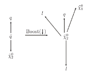
The $m_{lq}^{high}$ endpoint is conceptually much easier, however, as we only have to maximise the invariant mass that we can make from one of the leptons. The two sequential decays are shown in figure 3, where we show the effect of a boost from the $\tilde{q}$ rest frame to the $\tilde{\chi}_{2}^{0}$ rest frame. Any maximum in the $m_{lq}$ invariant mass must arise from having the relevant lepton (the ‘interesting lepton’) back to back with the quark in the $\tilde{\chi}^{0}_{2}$ rest frame. We can thus consider three extreme cases for the configuration of the leptons and $\tilde{\chi}_{1}^{0}$ in the $\tilde{\chi}_{2}^{0}$ rest frame:

Figure 3: The two rest frames involved in the squark cascade decay.

1. The $\tilde{\chi}^{0}_{1}$ is produced at rest, and the two leptons are back to back with one of them anti-parallel to the quark.

2. One of the leptons is produced at rest, and so the $\tilde{\chi}^{0}_{1}$ is produced back to back with the other lepton, with the interesting lepton being anti-parallel to the quark.

3. None of the particles from the three body decay is produced at rest, in which case we will get the highest invariant mass by having the interesting lepton emerging anti-parallel to the quark, and the other two particles travelling in the same direction as the quark.

Obtaining the $m_{lq}$ endpoint is simply a case of working out which of these gives the highest invariant mass. A short calculation gives us:

$$(m_{lq}^{2})^{\mbox{\tiny max}}_{\mbox{\tiny high}}=\frac{(m_{\tilde{q}}^{2}-m_{\tilde{\chi}^{0}_{2}}^{2})(m_{\tilde{\chi}^{0}_{2}}^{2}-m_{\tilde{\chi}^{0}_{1}}^{2})}{m_{\tilde{\chi}^{0}_{2}}^{2}}$$ (11)

The $m_{lq}^{low}$ endpoint is harder to obtain than the $m_{lq}^{high}$ endpoint, given that we want the maximum value of the smallest $m_{lq}$ invariant mass it is possible to form in an event. We apply a similar approach to that used in the previous subsection, and visualise the decay configuration that will give us the maximum before working out the endpoint.

In this case, we have proved that there is a local $m_{lq}^{low}$ maximum when the two leptons are produced parallel in the $\tilde{\chi}^{0}_{2}$ rest frame, travelling anti-parallel to the $\tilde{\chi}^{0}_{1}$ (which therefore travels parallel to the quark). Note that this does not exclude the possibility of other local maxima, but numerical simulation has not revealed any. We therefore take this configuration to give the global maximum of $m_{lq}^{low}$.

A short calculation gives:

$$(m_{lq}^{2})^{\mbox{\tiny max}}_{\mbox{\tiny low}}=\frac{(m_{\tilde{q}}^{2}-m_{\tilde{\chi}^{0}_{2}}^{2})(m_{\tilde{\chi}^{0}_{2}}^{2}-m_{\tilde{\chi}^{0}_{1}}^{2})}{2m_{\tilde{\chi}^{0}_{2}}^{2}}$$ (12)

3.5 Summary

Having obtained endpoints for the $m_{ll}$, $m_{llq}$, $m_{lq}^{high}$ and $m_{lq}^{low}$ distributions, we see that the expressions are very similar. The ratio of the $m_{lq}^{high}$ and $m_{lq}^{low}$ endpoint positions will always be $\sqrt{2}$, and, in a particular mass region, the $m_{llq}$ endpoint is coincident with the $m_{lq}^{high}$ endpoint. This ultimately means that there may not be enough information to precisely determine the mass differences involved in the decay chain, a point that will be discussed further in section 5.

4 Observation of three body endpoints in NUHM model

Having derived the endpoints for the process depicted in figure 2, we now discuss a concrete physics example by performing a Monte Carlo study of the NUHM model described in section 2.

4.1 Event generation and simulation

The mass spectrum and decay table of the NUHM point were taken from ISAJET 7.72 using the ISAWIG interface. We subsequently generated 3,300,000 signal events (corresponding to an integrated luminosity of $100\mbox{ fb}^{-1}$), using HERWIG 6.5 . This implements three body decays of SUSY particles with spin correlations, with the decays of interest here being:

1. $\tilde{\chi}_{2}^{0}\to Z\tilde{\chi}_{1}^{0}\to l^{+}l^{-}\tilde{\chi}_{1}^{0}$

2. $\tilde{\chi}_{2}^{0}\to l\tilde{l}\to l^{+}l^{-}\tilde{\chi}_{1}^{0}$

where the $Z$ and the slepton are off-shell. These generated events are then passed through the ATLFAST detector simulation (from the same release), whose jet cone algorithm used a cone with $\Delta R=0.4$. Electrons, muons and jets were subject to a minimum $p_{T}$ cut of 5, 6 and 10 GeV respectively.

We note that the ATLFAST reconstruction algorithms affect the ability to reconstruct leptons and jets in close proximity, and this is potentially a source of systematic error in our endpoints observations (particularly in the threshold position). This will also occur in full simulation, though to a lesser extent. A study of these systematic effects in both the fast and full simulation is long overdue, but is sufficiently complicated to warrant a separate publication. We note in passing that this affects all previous endpoint analyses, and is not specific to that considered here.

4.2 Selection cuts

In order to observe clear endpoints from the cascade decay process, it is necessary to first isolate a clean sample of squark decay events. One can select events with two OSSF leptons and a large amount of missing energy, and can also exploit the fact that one expects hard jets in SUSY events. Hence, all plots that follow are subject to the following cuts:

• $E_{T}^{\mbox{\tiny miss}}>300\mbox{ GeV;}$

• exactly two opposite-sign leptons with $p_{T}>5\mbox{ GeV}$ for electrons and $p_{T}>5\mbox{ GeV}$ for muons, with $|\eta|<2.5$;

• at least two jets with $p_{T}>150\mbox{ GeV}$;

The $E_{T}^{\mbox{\tiny miss}}$ and jet requirements should be sufficient to ensure that the events would be triggered by ATLAS. For example, these events should pass both specialised Supersymmetry trigger (“j70+xE70”: 1 jet $>$ 70 GeV and $E_{T}^{\mbox{\tiny miss}}>70$ GeV) and the inclusive missing energy trigger (“xE200”: $E_{T}^{\mbox{\tiny miss}}>200$ GeV) – see [14] and references therein. There are of course many SM processes that contribute to the dilepton background in any SUSY analysis, though it has been shown that these are highly suppressed once an OSSF cut is used in conjunction with cuts on lepton and jet $p_{T}$, and on missing energy. Although there is in principle still a tail of SM events that can contribute, it has found to be negligible in the past (see, for example, [15]), and a full study of this background is considered to be beyond the scope of this paper. We also note that the OSSF lepton signature can be produced by SUSY processes other than the decay of the $\tilde{\chi}_{2}^{0}$. However, a large fraction of such processes generate the two leptons with uncorrelated families, and so produce an equal number of opposite-sign opposite-flavour (OSOF) leptons. Thus one can “remove” this fraction (the majority) of the SUSY dilepton background by producing “flavour subtracted plots” in which one plots the combination $e^{+}e^{-}+\mu^{+}\mu^{-}-e^{+}\mu^{-}-e^{-}\mu^{+}$. Figures 8 to 11 below have all been flavour subtracted. Note that at the end of this flavour subtraction, a small number of events from SUSY processes producing dileptons of correlated flavour still remain. Events of this kind may be seen in the upper tail of figure 8. Note also that events in some of the plots below have been subjected to additional cuts (beyond the basic set detailed above). Where these additional cuts occur, they are explained in the text.

4.3 Note on endpoint positions

It should be remembered that the formulae for endpoint positions presented in section 3 take a squark mass as input. In reality not all squarks have the same mass, and so chains containing squarks with different masses will have endpoints at slightly different positions. This effect manifests itself as a smearing of the endpoints in any plots of experimental or simulated data. Plots of this kind are shown in section 4.4 and when indicating the positions at which endpoints are expected to be found in these plots, we are required to choose a “typical” squark mass for insertion into the relevant endpoint formula. We choose a 610 GeV “typical” squark mass for this purpose, although it should be borne in mind that the actual endpoints seen in the plots will be somewhat smeared due the the non-degeneracy of the squark masses contributing to them.

4.4 Invariant mass plots

4.4.1 $m_{ll}$ plot

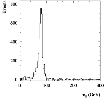
The $m_{ll}$ distribution is shown in figure 8; 4566 events survive after cuts and background subtraction, though it is noted that the effect of the trigger which may cut more harshly on lepton $p_{T}$ has not been considered. Using the mass spectrum given in section 2, we expect to find an endpoint at approximately 80 GeV, and this is clearly visible.

It is noted that the shape of the distribution is very different from the triangular shape normally encountered in the case of successive two body decays resulting from the phase space for that process, and this might prove important when attempting to distinguish three body from two body decays. This is considered further in section 5.

4.4.2 $m_{llq}$ plots

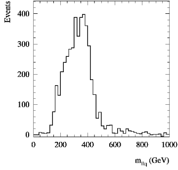
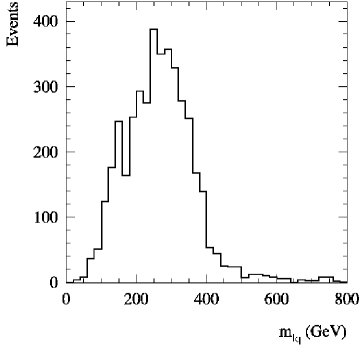
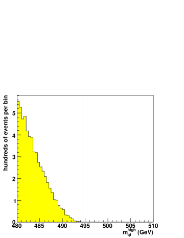
As soon as we start to form invariant masses involving quarks, it is important to consider how to select the correct quark from the cascade decay. A reasonable assumption is that the two hardest jets in the event will come from squark decay on either side of the event, and if we take the lowest of the two $m_{llq}$ invariant masses formed from the two hardest jets in the event, this should lie below the $m_{llq}$ endpoint. The distribution of this $m_{llq}$ is shown in figure 8, and there is a visible endpoint consistent with the predicted value of approximately 490 GeV. The plot contains the same number of events as the $m_{ll}$ plot, as the cuts are the same.

In order to obtain a further constraint on the physical model underlying the data, we construct a threshold in the $m_{llq}$ distribution. We follow the convention used in the study of successive two body decays, and choose to look at the subset of events for which $m_{ll}>m_{ll}^{max}/\sqrt{2}$. Substituting $m_{ll}^{max}/\sqrt{2}$ in place of $L_{m}$ in equation 10 gives the following threshold:

$$(m_{llq}^{min})^{2}=\frac{(\sqrt{a}-\sqrt{z})^{2}}{2}+\frac{(c-a)}{4a}\left(3a-z-2\sqrt{az}-\sqrt{a^{2}+z^{2}+4\sqrt{az}(a+z)-10az}\right)$$ (13)

where $c=m_{\tilde{q}}^{2}$, $a=m_{\tilde{\chi}_{2}^{0}}^{2}$ and $z=m_{\tilde{\chi}_{1}^{0}}^{2}$. Traditionally (i.e. in chains with successive two-body decays) this additional constraint requires, somewhat arbitrarily, that the angular separation of the two leptons in the rest frame of the slepton be greater than than a right angle. For the three-body neutralino decay considered in this paper, that geometrical interpretation is lost, but this is of no consequence to us.

A plot of the $m_{llq}$ distribution is given in figure 9, where we note that, because we are looking for a threshold, the highest of the two $m_{llq}$ invariant masses formed with the two hardest jets in the event is used to make the plot. 4172 events are contained in the plot. A threshold structure of some form is clearly observed, though it is difficult to ascertain the precise position, as the shape of the edge is not yet a well understood function of the sparticle masses and cut-induced ‘detector’ effects. To use the constraint from this edge to the full, it may be necessary to repeat the analysis of [16] in the context of a three-body final decay. The predicted value is approximately 240 GeV.

4.4.3 $m_{lq}$ plots

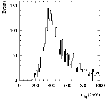
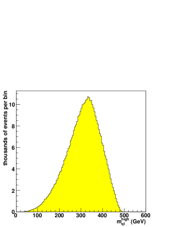
The $m_{lq}^{\tiny{high}}$ distribution is plotted by forming $m_{llq}$ invariant masses with the two hardest jets in the event. The jet from the lowest mass combination (which is our best guess for the quark emitted in the squark cascade decay) is then used to form the $m_{lq}$ invariant mass with each of the leptons in the events. The maximum of these is plotted in the $m_{lq}^{\mbox{\tiny high}}$ plot (shown in figure 11), where we note that we have used the additional cut that the dilepton invariant mass in each selected event must be less than the dilepton endpoint. 4161 events are in the plot. There is an endpoint predicted at about 490 GeV (we are in the mass region where it should appear at the same position as the $m_{llq}$ endpoint) and this is consistent with the plot, though it is difficult to identify the endpoint due the fact that the shape is easily confused with the tail. It is easier to see why this is the case by looking at the distribution in a simpler context, namely one that ignores all detector effects and which looks only at phase space which we have implemented using a “toy” Monte Carlo. In this, we also ignore the smearing coming from the spread in squark masses which is normally present, by generating chains with a single squark mass. Using this toy Monte Carlo we generate plots of the distribution in the vicinity of the edge (figures 13 and 13) and we see that the endpoint is only approached quadratically. Although a full analysis of the tail would probably require full simulation (and thus a separate study), we have attempted to determine how much is caused by detector smearing, and how much is caused by background SUSY processes. Figures 5 to 6 examine the $m_{eq}^{\tiny{high}}$ distribution, showing the Monte Carlo truth plot, the plot obtained by selecting events on the basis of truth but with the particles reconstructed by the ATLFAST detector simulation, and finally a plot which contains only SUSY background processes. We see that the tail does not predominantly arise from detector smearing (which will nevertheless smear the endpoint), but has instead a large contribution from the SUSY background. There is also a combinatoric background related to the wrong choice of squark, but this is harder to isolate.

Figure 4: The truth distribution for the $m_{eq}^{\tiny{high}}$ invariant mass, taken from the Herwig event record as recorded in ATLFAST . The exhibits a clean edge with no tail.

Figure 5: The $m_{eq}^{\tiny{high}}$ distribution obtained by selecting events on the basis of Monte Carlo truth information, but with the electrons and jets reconstructed by ATLFAST . We see that the plot has a slightly higher endpoint than the truth distribution, but no significant tail.

Figure 6: The $m_{eq}^{\tiny{high}}$ distribution obtained using events with no decay of the form $\tilde{\chi}_{2}^{0}\to\tilde{\chi}_{1}^{0}e^{+}e^{-}$, representing the contribution to the plot from SUSY background processes.

The $m_{lq}^{\mbox{\tiny low}}$ plot is constructed in a similar fashion to the $m_{lq}^{\mbox{\tiny high}}$ plot, with the exception that we take the lowest of the two possible $m_{lq}$ combinations in each event. The result is shown in figure 11, where we have used an additional cut; one of the $m_{llq}$ invariant masses formed from the two hardest jets in the event must lie below the approximate observed position of the $m_{llq}$ endpoint, and one must lie above, leaving 1664 events in the plot. This removes much of the tail due to incorrect squark choice, and leaves us with a very clean endpoint at the predicted value of approximately 350 GeV.

Figure 7: The $m_{ll}$ distribution for the NUHM model defined in the text, with flavour subtraction.

Figure 8: The flavour subtracted $m_{llq}$ distribution for the NUHM model defined in the text, constructed by taking the lowest $m_{llq}$ invariant mass that can be formed from the two hardest jets in the event.

Figure 9: The flavour subtracted $m_{llq}$ threshold plot, constructed using the highest of the $m_{llq}$ invariant masses that can be formed from the two hardest jets in each selected event.

Figure 10: The flavour subtracted $m_{lq}^{high}$ distribution for the NUHM model defined in the text, constructed by taking the jet (from the two hardest jets in the event) that gives the lowest $m_{llq}$ invariant mass and forming the highest invariant mass that one can make with the two leptons in the event.

Figure 11: The flavour subtracted $m_{lq}^{low}$ distribution for the NUHM model defined in the text, constructed by taking the jet (from the two hardest jets in the event) that gives the lowest $m_{llq}$ invariant mass and forming the highest invariant mass that one can make with the two leptons in the event.

Figure 12: A toy Monte Carlo calculation of the shape of an example $m_{lq}^{high}$ distribution (for particle masses of $m_{{{\tilde{\chi}}_{1}^{0}}}=95$ GeV, $m_{{{\tilde{\chi}}_{2}^{0}}}=179$ GeV and $m_{{{\tilde{q}}}}=610$ GeV similar to those in the NUHM model defined in the text) using the approximation in which all particles are taken to be scalars, i.e. phase-space only. The calculation assumes 100% acceptance and does not model any detector effects. $m_{lq}^{high}$ values are in GeV.

Figure 13: A zoomed view of the $m_{lq}^{high}$ phase space distribution (left) in the vicinity of the end point $(m_{lq})^{max}_{high}$, the position of which is given by the vertical line at 494.24 GeV. $m_{lq}^{high}$ values are in GeV.

5 Discussion

Having collected a series of endpoint plots and derived their positions in terms of the sparticle masses involved in our decay chain, we ought in principle to be able to reconstruct the masses in the chain. This is not as simple as it first appears, however, for the following reasons:

1. Our NUHM point is in the mass region where the $m_{lq}^{high}$ endpoint is in the same position as the $m_{llq}$ endpoint, and we also know that the $m_{lq}^{low}$ edge is related to these other two merely through multiplication by a constant factor. Discounting the poorly measured threshold, we thus only have two equations in three unknowns (we can use the $m_{ll}$ endpoint as our second equation), and we do not have enough information to constrain the masses.

2. The observation of endpoints does not reveal anything about the decay process that produces them, and the shapes of the lepton-jet invariant mass distributions in this paper are not dissimilar to those produced by chains of successive two body decays. Hence, we need to consider how we would in principle distinguish between the two cases to be certain that we are reconstructing the correct masses.

Given that the purpose of this note is simply to present a derivation of the three body endpoint expressions and demonstrate their existence in a SUSY model, we will not implement solutions to either of these problems. However, the following discussion will suggest possible answers to both.

5.1 Mass reconstruction

In order to reconstruct the sparticle masses in our process, we will need to supply extra constraints. One possible method involves going one step higher in the decay chain, and searching for decays of the form:

$$\tilde{g}\rightarrow\tilde{q}q\rightarrow\tilde{\chi}_{2}^{0}qq\rightarrow\tilde{\chi}_{1}^{0}qqll$$ (14)

This will give us more endpoints, and hence we will obtain direct constraints on the masses of the system. This is similar to an approach used for two body decays in [17], and would have the advantage of providing a measurement of the gluino mass. The problem here is that our NUHM model has a relatively light gluino, which is lighter than the squarks of the first two generations. Hence, the method will only be applicable to decay chains involving stop and sbottom squarks, and we see that whilst this approach may be helpful in some cases it is certainly not generally applicable to all regions of parameter space.

Another approach is to use other observables to constrain sparticle masses. Our previous work in [6] demonstrated that one can obtain a dramatic improvement in mass measurements by combining exclusive data (such as endpoint information) with inclusive observables (such as the cross-section of events passing a missing $p_{T}$ cut, to give one example). This analysis could be repeated here, and with enough inclusive observables one could obtain good measurements of the sparticle masses involved in our cascade process. This has the advantage of being generally applicable regardless of the mass spectrum, though it relies on specifying a particular SUSY model in which to perform the analysis.

5.2 Decay chain ambiguity

We have already remarked that it is not trivial to distinguish three body endpoints from two body endpoints, and hence the observation of endpoints alone is not enough to be able to reconstruct masses. Even assuming that we $do$ have a way to do this, we can in general exchange the neutralinos in our decay process for other neutralinos without changing the observed signature, and so one cannot assume that we know exactly which process is causing the observed edges. This latter point was previously considered by us in [6] for the case of two body decays, and here we will concern ourselves with the former question of distinguishing between two and three body decays.

In the previous sections we have already seen one characteristic feature of three body decay chains; the ratio of the $m_{llq}$ and $m_{lq}^{low}$ endpoint positions is always $\sqrt{2}$. Provided one can obtain precise measurements of these quantities, we would have a clue that we were looking at three body processes, although this could easily be faked by two body decays that conspired to produce endpoints in similar positions.

For an extra clue, consider that although the shapes of the lepton-jet distributions in three body decays are not dissimilar to those encountered in two body processes, this is not true of the $m_{ll}$ distribution, and hence there is potentially some information contained in the shape of the dilepton distribution. In the two-body case, one obtains a triangular shape that is identical to the phase space distribution. In contrast, the three-body distribution in figure 8 is heavily peaked toward the endpoint. Unfortunately, this is unlikely to be true over the whole of parameter space; the three body decay proceeds via an off-shell Z or slepton, and the $m_{ll}$ distribution is peaked toward the endpoint when the endpoint (which is the same as the mass difference between the $\tilde{\chi}_{2}^{0}$ and the $\tilde{\chi}_{1}^{0}$) approaches, for example, the Z mass, such that the shape will depend heavily on the SUSY point. Furthermore, a previous study investigated the effect on the $m_{ll}$ shape of incorporating the matrix element for the three body decay process in addition to the phase space, for different points in mSUGRA parameter space, and although for some points it dramatically altered the pure phase space result there were other points where the three body and phase space shapes were virtually indistinguishable [18].

To summarise, we may be fortunate enough to find that nature presents a point at which we can distinguish three body decays from two body processes simply by looking at the endpoint shapes and positions, but this is certainly not guaranteed. For this reason, a better approach to the problem of mass reconstruction is to use the Markov Chain techniques presented in [6], where no assumption is made about the processes causing the observed endpoints. This allows us to select a region of the parameter space consistent with the data which can be used as a basis for further investigation.

6 Conclusions

We have derived expressions for the position of the kinematic endpoints arising in cascade decays featuring a two body decay followed by a three body decay, and have applied them to the lepton-jet invariant mass distributions given by a squark decay process. We have performed the first analysis of an NUHM model as it would appear within the ATLAS detector, and, using standard cuts, have observed endpoints that are consistent with the predicted positions. We thus conclude that the technique is a viable extension of the current method used in chains of two body decays.

We have discussed the problem of mass reconstruction in models with a similar phenomenology, and have found that it is hampered by both a lack of constraint from the endpoint equations themselves, and the problem of distinguishing three body from two body decay processes. In the case of the NUHM benchmark point $\gamma$, one would be able to identify the decays as three body decays by using the shape of the dilepton invariant mass distribution.

7 Acknowledgements

We owe thanks to the other members of the Cambridge Supersymmetry Working Group, in particular Peter Richardson for information regarding the HERWIG treatment of three-body neutralino decays. We acknowledge Borge Gjelsten, whom we understand has independently calculated endpoints for three body decays, but has not yet published them. This work has been performed within the ATLAS Collaboration. We have made use of ATLFAST which is the result of collaboration-wide efforts within ATLAS. We thank ATLAS collaboration members for useful discussions, and in particular wish to thank Paul de Jong and an anonymous “ATLAS Scientific Note referee” for bringing important issues to our attention.

References

- [1] S. P. Martin, A supersymmetry primer, hep-ph/9709356.
- [2] B. C. Allanach, C. G. Lester, M. A. Parker, and B. R. Webber, Measuring sparticle masses in non-universal string inspired models at the LHC, JHEP 09 (2000) 004, [hep-ph/0007009].
- [3] ATLAS Collaboration, ATLAS detector and physics performance Technical Design Report. CERN/LHCC 99-15, 1999.
- [4] C. G. Lester, Model independent sparticle mass measurements at ATLAS, . CERN-THESIS-2004-003 – http://cdsweb.cern.ch/search.py?sysno=002420651CER.
- [5] I. Borjanović, J. Krstić, and D. Popović, SPS 5 mSUGRA studies at ATLAS, ATLAS Physics note (2005) ATL–PHYS–INT–2005–001.
- [6] C. G. Lester, M. A. Parker, and M. J. White, Determining SUSY model parameters and masses at the LHC using cross-sections, kinematic edges and other observables, JHEP 01 (2006) 080, [hep-ph/0508143].
- [7] N. Ozturk, SUSY searches at the LHC, ATLAS Physics note (2005) ATL–PHYS–CONF–2005–007.
- [8] T. Lari, SUSY studies with ATLAS: hadronic signatures and focus point, ATLAS Physics note (2004) ATL–PHYS–CONF–2005–002.
- [9] G. Comune, SUSY with ATLAS: Leptonic signatures, coannihilation region, ATLAS Physics note (2004) ATL–PHYS–CONF–2005–003.
- [10] A. De Roeck et al., Supersymmetric benchmarks with non-universal scalar masses or gravitino dark matter, hep-ph/0508198.
- [11] H. Baer, A. Mustafayev, S. Profumo, A. Belyaev, and X. Tata, Direct, indirect and collider detection of neutralino dark matter in SUSY models with non-universal higgs masses, JHEP 07 (2005) 065, [hep-ph/0504001].
-
[12]
F. E. Paige and S. D. Protopopescu, ISAJET 7.72: A Monte Carlo event
generator for , and reactions.
http://www.phy.bnl.gov/~isajet/, 2005. - [13] S. Moretti, K. Odagiri, P. Richardson, M. H. Seymour, and B. R. Webber, Implementation of supersymmetric processes in the HERWIG event generator, JHEP 04 (2002) 028, [hep-ph/0204123].
- [14] T. Schörner-Sadenius and S. Tapprogge, ATLAS trigger menus for the LHC start-up phase, ATLAS Physics note (2003). CERN-ATL-DAQ-2003-004 ATL-DAQ-2003-004 http://cdsweb.cern.ch/search.py?recid=685479.
- [15] I. Hinchliffe, F. E. Paige, M. D. Shapiro, J. Soderqvist, and W. Yao, Precision SUSY measurements at LHC, Phys. Rev. D55 (1997) 5520–5540, [hep-ph/9610544].
- [16] C. G. Lester, Constrained invariant mass distributions in cascade decays: The shape of the ‘m(qll)-threshold’ and similar distributions, hep-ph/0603171.
- [17] B. K. Gjelsten, D. J. Miller, and P. Osland, Measurement of the gluino mass via cascade decays for SPS 1a, JHEP 06 (2005) 015, [hep-ph/0501033].
- [18] S. Chouridou, R. Strhmer, and T. Trefzger, Study of the three body matrix element of the neutralino decay , ATLAS Physics note (2003) ATL–COM–PHYS–2002–032.