Abstract

I present a calculation of threshold soft-gluon corrections to single top quark production in $p{\bar{p}}$ collisions via all partonic processes in the $t$ and $s$ channels and via associated top quark and $W$ boson production. The soft-gluon corrections are formally resummed to all orders, and finite-order expansions of the resummed cross section are calculated through next-to-next-to-next-to-leading order (NNNLO) at next-to-leading logarithmic (NLL) accuracy. Numerical results for single top quark production at the Tevatron are presented, including the dependence of the cross sections on the top quark mass and on the factorization and renormalization scales. The threshold corrections in the $t$ channel are small while in the $s$ channel they are large and dominant. Associated $tW$ production remains relatively minor due to the small leading-order cross section even though the $K$ factors are large.

1 Introduction

The top quark was discovered in 1995 by the CDF and D0 collaborations at the Tevatron in top-antitop quark pair production events [1, 2]. The search for single top quark events continues intensively at the Tevatron [3, 4]. The theoretical cross section is less than that of the $t{\bar{t}}$ cross section and the backgrounds make the extraction of the signal challenging.

Single top quark production provides opportunities for the study of the electroweak properties of the top quark (such as a direct measurement of the $V_{tb}$ CKM matrix element), for further insights into electroweak theory since the top quark mass is of the same order of magnitude as the electroweak symmetry breaking scale, as well as for the possible discovery of new physics (extra quarks or gauge bosons, modified top quark interactions, etc.) (see, for example, Refs. [5-11]).

The production of single top quarks can proceed through three distinct partonic processes. One of them is the $t$-channel process that proceeds via the exchange of a space-like $W$ boson (Fig. 1), a second is the $s$-channel process that proceeds via the exchange of a time-like $W$ boson (Fig. 2), and a third is associated $tW$ production (Fig. 3). In the $t$ channel we have processes of the form $qb\rightarrow q^{\prime}t$ and ${\bar{q}}b\rightarrow{\bar{q}}^{\prime}t$, such as $ub\rightarrow dt$ and ${\bar{d}}b\rightarrow{\bar{u}}t$ as well as processes involving the charm quark and Cabibbo-supressed contributions. In the $s$ channel we have processes of the form $q{\bar{q}}^{\prime}\rightarrow{\bar{b}}t$, such as $u{\bar{d}}\rightarrow{\bar{b}}t$ as well as processes involving the charm quark and Cabibbo-supressed contributions. Associated production of a top quark and a $W$ boson proceeds via $bg\rightarrow tW^{-}$ as well as Cabibbo-supressed contributions.

At the Tevatron the $t$-channel process is numerically dominant, the $s$-channel process is smaller, and associated $tW$ production is quite minor. Although we will be discussing the production of a top quark in this paper we note that the corresponding cross sections for the production of an antitop quark at the Tevatron are identical. Calculations of NLO corrections to single top production via the various partonic modes have appeared in Refs. [12-20].

The cross section for single top quark production in proton-antiproton collisions is

$$\sigma=\sum_{f}\int dx_{1}dx_{2}\,\phi_{f_{1}/p}(x_{1},\mu_{F})\,\phi_{f_{2}/{\bar{p}}}(x_{2},\mu_{F})\,{\hat{\sigma}}(s,t,u,\mu_{F},\mu_{R},\alpha_{s})\,,$$ (1.1)

where $\phi_{f_{1}/p}$ ($\phi_{f_{2}/{\bar{p}}}$) is the distribution function for parton $f_{1}$ ($f_{2}$) carrying momentum fraction $x_{1}$ ($x_{2}$) of the proton (antiproton), $\mu_{F}$ is the factorization scale, and $\mu_{R}$ is the renormalization scale. The parton-level cross section is denoted by ${\hat{\sigma}}$ and can be written as a perturbative expansion in the strong coupling $\alpha_{s}$, and $s$, $t$, $u$ are standard kinematical invariants formed from the momenta of the particles in the hard scattering.

Near kinematical threshold for the production of a specified final state, such as a single top quark, large corrections appear from soft-gluon emission [21, 22, 23, 24]. These corrections arise from incomplete cancellations of infrared divergences between virtual diagrams and real diagrams with soft (i.e. low-energy) gluons. In principle one can obtain the form of these soft radiative corrections at any order in $\alpha_{s}$ and formally resum them to all orders. However in practice such resummed cross sections depend on a prescription to avoid the infrared singularity and ambiguities from prescription dependence can actually be larger than contributions from high-order terms [24]. Hence, we provide fixed-order expansions of the resummed cross section, as has been done for many other processes [10, 24, 25, 26, 27, 28, 29], in order to avoid such ambiguities. We will calculate soft-gluon corrections for single top quark production through NNNLO at NLL accuracy.

Figure 1: Leading-order $t$-channel diagram for single top quark production.

Figure 2: Leading-order $s$-channel diagram for single top quark production.

Figure 3: Leading-order associated $tW$ production diagram for single top quark production.

In Section 2 we briefly describe the threshold resummation formalism and provide expressions for the resummed cross section. In Section 3 we expand the resummed cross section in powers of $\alpha_{s}$ and provide formulas for the soft-gluon corrections through NNNLO. In Section 4 we present numerical results for single top quark production via the $t$ channel at the Tevatron. Analogous results are provided for the $s$ channel in Section 5 and for associated $tW$ production in Section 6. The conclusion is in Section 7, and the Appendix collects formulas and details on the kinematics and on electroweak parameters used in the calculations.

2 Threshold resummation

In this section we present the analytical form of the resummed cross section for single top quark production. Details of the general resummation formalism for hard-scattering cross sections have been presented elsewhere [21, 22, 23, 24, 29, 30] so here we explicitly show only the expressions directly relevant to single top quark production.

For the process $p_{1}+p_{2}\rightarrow p_{3}+p_{4}$ (where the particles are represented by their momenta $p_{i}$), the partonic kinematical invariants are $s=(p_{1}+p_{2})^{2}$, $t=(p_{1}-p_{3})^{2}$, $u=(p_{2}-p_{3})^{2}$, $s_{4}=s+t+u-m_{3}^{2}-m_{4}^{2}$. Note that we ignore the mass of the $b$-quark in the kinematics. Near threshold, i.e. when we have just enough partonic energy to produce the final state, $s_{4}\rightarrow 0$. The threshold corrections then take the form of logarithmic plus distributions, $[\ln^{l}(s_{4}/m_{t}^{2})/s_{4}]_{+}$, where $l\leq 2n-1$ for the $n$-th order QCD corrections and $m_{t}$ is the top quark mass. These plus distributions are defined through their integral with any smooth function, such as parton distributions, giving a finite result [21, 30].

The resummation of threshold logarithms is carried out in moment space and it follows from the refactorization of the cross section into hard, soft, and jet functions that describe, respectively, the hard scattering, noncollinear soft gluon emission, and collinear gluon emission from the partons in the scattering [21, 22, 23]. We define moments of the partonic cross section by ${\hat{\sigma}}(N)=\int(ds_{4}/s)\;e^{-Ns_{4}/s}{\hat{\sigma}}(s_{4})$, with $N$ the moment variable. Under moments logarithms of $s_{4}$ transform into logarithms of $N$, which exponentiate. The resummed partonic cross section in moment space [21, 22, 23, 30] is then given by

$${\hat{\sigma}}^{res}(N) = \exp\left[\sum_{i}E^{f_{i}}(N_{i})\right]\;\exp\left[\sum_{j}{E^{\prime}}^{f_{j}}(N_{j})\right]\;\exp\left[\sum_{i}2\int_{\mu_{F}}^{\sqrt{s}}\frac{d\mu}{\mu}\;\gamma_{i/i}\left(N_{i},\alpha_{s}(\mu)\right)\right]\;$$

$$\times\,\exp\left[\sum_{i}2d_{\alpha_{s}}\int_{\mu_{R}}^{\sqrt{s}}\frac{d\mu}{\mu}\;\beta\left(\alpha_{s}(\mu)\right)\right]\;H^{f_{i}f_{j}}\left(\alpha_{s}(\mu_{R})\right)$$

$$\times\,\exp\left[\int_{\sqrt{s}}^{{\sqrt{s}}/{\tilde{N}_{j}}}\frac{d\mu}{\mu}\;\Gamma_{S}^{\dagger\,f_{i}f_{j}}\left(\alpha_{s}(\mu)\right)\right]\;{\tilde{S}^{f_{i}f_{j}}}\left(\alpha_{s}\left(\frac{\sqrt{s}}{\tilde{N}_{j}}\right)\right)\;\exp\left[\int_{\sqrt{s}}^{{\sqrt{s}}/{\tilde{N}_{j}}}\frac{d\mu}{\mu}\;\Gamma_{S}^{f_{i}f_{j}}\left(\alpha_{s}(\mu)\right)\right]\,.$$

The first exponent resums collinear and soft gluon emission from the incoming partons in the hard scattering and is given in the $\overline{\rm MS}$ scheme by

$$\sum_{i}E^{f_{i}}(N_{i})=-C_{i}\sum_{i}\int^{1}_{0}dz\frac{z^{N_{i}-1}-1}{1-z}\;\left\{\int^{1}_{(1-z)^{2}}\frac{d\lambda}{\lambda}\frac{\alpha_{s}(\lambda s)}{\pi}+\frac{\alpha_{s}((1-z)^{2}s)}{\pi}\right\}+{\cal O}(\alpha_{s}^{2})\,.$$ (2.2)

Here $N_{1}=N[(-u+m_{t}^{2})/m_{t}^{2}]$ and $N_{2}=N[(-t+m_{t}^{2})/m_{t}^{2}]$ for incoming partons $i=1,2$, $C_{i}=C_{F}=(N_{c}^{2}-1)/(2N_{c})$ for quarks, with $N_{c}$ the number of colors, and $C_{i}=C_{A}=N_{c}$ for gluons.

The second exponent resums collinear and soft gluon emission from the outgoing massless partons, if any (none in associated production), in the hard scattering and is given in the $\overline{\rm MS}$ scheme by

$${E^{\prime}}^{f_{j}}(N_{j}) \!\!= \!\!\int^{1}_{0}dz\frac{z^{N_{j}-1}-1}{1-z}\;\left\{C_{j}\int^{1-z}_{(1-z)^{2}}\frac{d\lambda}{\lambda}\frac{\alpha_{s}\left(\lambda s\right)}{\pi}-B_{j}^{(1)}\frac{\alpha_{s}((1-z)s)}{\pi}-C_{j}\frac{\alpha_{s}((1-z)^{2}s)}{\pi}\right\}$$ (2.3)

$$+{\cal O}(\alpha_{s}^{2})\,.$$

Here $N_{j}=N(s/m_{t}^{2})$, and $B_{j}^{(1)}$ equals $3C_{F}/4$ for quarks and $\beta_{0}/4$ for gluons, with $\beta_{0}=(11C_{A}-2n_{f})/3$ the lowest-order term in the expansion of the $\beta$-function, $\beta(\alpha_{s})\equiv\mu d\ln g/d\mu=-\beta_{0}\alpha_{s}/(4\pi)+{\cal O}(\alpha_{s}^{2})$, where $n_{f}$ is the number of light quark flavors.

In the third exponent, the parton anomalous dimensions are given by $\gamma_{q/q}(N_{i},\alpha_{s})=$
$(\alpha_{s}/\pi)[3C_{F}/4-C_{F}\ln N_{i}]+{\cal O}(\alpha_{s}^{2})$ for quarks and $\gamma_{g/g}(N_{i},\alpha_{s})=(\alpha_{s}/\pi)[\beta_{0}/4-C_{A}\ln N_{i}]+{\cal O}(\alpha_{s}^{2})$ for gluons, and $\mu_{F}$ is the factorization scale.

In the fourth exponent the $\beta$ function is as described above, the constant $d_{\alpha_{s}}=0$ or 1 if the leading order cross section is of order $\alpha_{s}^{0}$ ($t$ and $s$ channels) or $\alpha_{s}^{1}$ (associated $tW$ production) respectively, and $\mu_{R}$ is the renormalization scale.

$H^{f_{i}f_{j}}$ are the hard-scattering functions for the scattering of partons $f_{i}$ and $f_{j}$, while $S^{f_{i}f_{j}}$ are the soft functions describing noncollinear soft gluon emission [21]. We use the expansions $H=H^{(0)}+(\alpha_{s}/\pi)H^{(1)}+{\cal O}(\alpha_{s}^{2})$ and $S=S^{(0)}+(\alpha_{s}/\pi)S^{(1)}+{\cal O}(\alpha_{s}^{2})$. Also ${\tilde{N}}=Ne^{\gamma_{E}}$, with $\gamma_{E}$ the Euler constant. At lowest order, the product of $H^{f_{i}f_{j}}$ and $S^{f_{i}f_{j}}$ reproduces the Born cross section for each partonic process, $\sigma^{B}=\alpha_{s}^{d_{\alpha_{s}}}H^{(0)}S^{(0)}$.

The evolution of the soft function follows from its renormalization group properties and is given in terms of the soft anomalous dimension $\Gamma_{S}^{f_{i}f_{j}}$ [21, 22, 31]. We expand $\Gamma_{S}=(\alpha_{s}/\pi)\Gamma_{S}^{(1)}+{\cal O}(\alpha_{s}^{2})$. The one-loop term $\Gamma_{S}^{(1)}$ is determined through the explicit calculation, in the eikonal approximation, of the one-loop diagrams involving eikonal vertex corrections as well as top quark self-energies as shown in Figs. 4-7 (for the requisite integrals in dimensional regularization see [21]). Here the partons in the scattering are represented by eikonal lines that connect in a color vertex. Explicit expressions for the soft anomalous dimensions in the various channels are given in the next section.

Figure 4: One-loop eikonal vertex corrections to the soft function for the $t$-channel diagram in single top quark production.

Figure 5: One-loop eikonal vertex corrections to the soft function for the $s$-channel diagram in single top quark production.

Figure 6: One-loop eikonal vertex corrections to the soft function for the associated $tW$ production diagram in single top quark production.

Figure 7: Top-quark eikonal self-energy one-loop corrections in single top quark production: (a) $t$ channel; (b) $s$ channel; (c) associated $tW$ production.

By expanding the resummed cross section, Eq. (LABEL:resHS), in powers of $\alpha_{s}$ we derive fixed-order corrections in the perturbative series that do not involve the prescription ambiguity that a fully resummed cross section entails [24]. In the $n$-th order corrections, the leading logarithms (LL) are those with $l=2n-1$ while the next-to-leading logarithms (NLL) are those with $l=2n-2$. In this paper we calculate next-to-leading order (NLO), next-to-next-to-leading order (NNLO), and NNNLO soft-gluon threshold corrections at NLL accuracy, i.e. at each order including both leading and next-to-leading logarithms, and also consistently including terms that involve the factorization and renormalization scales and $\zeta$ constants, which arise from the inversion from moment space where the resummation is performed back to momentum space. We denote these corrections as NLO-NLL, NNLO-NLL, and NNNLO-NLL, respectively. Full details are given in the next section (see also Refs. [24, 30]).

3 NNNLO soft-gluon corrections

We now proceed with the calculation of the NLO, NNLO, and NNNLO soft-gluon corrections at NLL accuracy by expanding the resummed cross section, Eq. (LABEL:resHS). In our derivation of these corrections we follow the general techniques and master formulas presented in Ref. [30].

The NLO soft-gluon corrections at NLL accuracy for the processes are

$$\frac{d^{2}{\hat{\sigma}}^{(1)}}{dt\,du}=F^{B}\frac{\alpha_{s}(\mu_{R}^{2})}{\pi}\left\{c_{3}\left[\frac{\ln(s_{4}/m_{t}^{2})}{s_{4}}\right]_{+}+c_{2}\left[\frac{1}{s_{4}}\right]_{+}+c_{1}^{\mu}\,\delta(s_{4})\right\}\,,$$ (3.1)

where $F_{B}$ is the Born term defined in the Appendix, Eq. (A.9).

For the $t$ and $s$ channels the LL coefficient is $c_{3}^{t,s}=3C_{F}$ while for associated $tW$ production it is $c_{3}^{tW}=2(C_{F}+C_{A})$.

The NLL coefficient, $c_{2}$, can be written as $c_{2}=T_{2}+c_{2}^{\mu}$, where $T_{2}$ represents the scale-independent part of $c_{2}$ and $c_{2}^{\mu}$ has all the scale dependence. For the $t$ and $s$ channels,

$$T_{2}^{t,s}=2{\rm Re}{\Gamma^{\prime}}_{S}^{(1)\;t,s}-\frac{15}{4}C_{F}-2C_{F}\ln\left(\frac{(t-m^{2}_{t})(u-m^{2}_{t})}{m_{t}^{4}}\right)-3C_{F}\ln\left(\frac{m_{t}^{2}}{s}\right)$$ (3.2)

and

$$c_{2}^{\mu\;t,s}=-2C_{F}\ln\left(\frac{\mu_{F}^{2}}{m_{t}^{2}}\right)\,,$$ (3.3)

while for associated $tW$ production,

$$T_{2}^{tW} = 2{\rm Re}{\Gamma^{\prime}}_{S}^{(1)\;tW}-C_{F}-C_{A}-2C_{F}\ln\left(\frac{-u+m^{2}_{W}}{m_{t}^{2}}\right)-2C_{A}\ln\left(\frac{-t+m^{2}_{W}}{m_{t}^{2}}\right)$$ (3.4)

$$\hskip 14.22636pt{}-(C_{F}+C_{A})\ln\left(\frac{m_{t}^{2}}{s}\right),$$

with $m_{W}$ the $W$-boson mass, and

$$c_{2}^{\mu\;tW}=-(C_{F}+C_{A})\ln\left(\frac{\mu_{F}^{2}}{m_{t}^{2}}\right)\,.$$ (3.5)

The term ${\rm Re}{\Gamma^{\prime}}_{S}^{(1)}$ denotes the real gauge-independent part of the one-loop soft anomalous dimension (gauge-dependent terms cancel out in the cross section). A one-loop calculation gives for the $t$ channel (Figs. 4, 7a)

$${\rm Re}{\Gamma^{\prime}}_{S}^{(1)\;t}=C_{F}\left[\ln\left(\frac{-t}{s}\right)+\ln\left(\frac{m_{t}^{2}-t}{m_{t}\sqrt{s}}\right)+1\right]\,,$$ (3.6)

for the $s$ channel (Figs. 5, 7b)

$${\rm Re}{\Gamma^{\prime}}_{S}^{(1)\;s}=C_{F}\left[\ln\left(\frac{s-m_{t}^{2}}{m_{t}\sqrt{s}}\right)+1\right]\,,$$ (3.7)

and for associated $tW$ production (Figs. 6, 7c)

$${\rm Re}{\Gamma^{\prime}}_{S}^{(1)\;tW}=C_{F}\ln\left(\frac{m_{t}^{2}-t}{m_{t}\sqrt{s}}\right)+\frac{C_{A}}{2}\ln\left(\frac{m_{t}^{2}-u}{m_{t}^{2}-t}\right)+\frac{C_{A}}{2}\,.$$ (3.8)

The coefficient $c_{1}^{\mu}$ in Eq. (3.1) represents the scale-dependent part of the $\delta(s_{4})$ corrections. For the $t$ and $s$ channels

$$c_{1}^{\mu\;t,s}=\left[C_{F}\ln\left(\frac{(t-m^{2}_{t})(u-m^{2}_{t})}{m_{t}^{4}}\right)-\frac{3}{2}C_{F}\right]\ln\left(\frac{\mu_{F}^{2}}{m_{t}^{2}}\right)\,,$$ (3.9)

and for associated $tW$ production

$$c_{1}^{\mu\;tW} = \left[C_{F}\ln\left(\frac{-u+m^{2}_{W}}{m_{t}^{2}}\right)+C_{A}\ln\left(\frac{-t+m^{2}_{W}}{m_{t}^{2}}\right)-\frac{3}{4}C_{F}-\frac{\beta_{0}}{4}\right]\ln\left(\frac{\mu_{F}^{2}}{m_{t}^{2}}\right)$$ (3.10)

$$\hskip 14.22636pt{}+\frac{\beta_{0}}{4}\ln\left(\frac{\mu_{R}^{2}}{m_{t}^{2}}\right)\,.$$

Note that we do not calculate the virtual corrections here. Our calculation of the NLO soft-gluon corrections includes the full leading and next-to-leading logarithms and is thus a NLO-NLL calculation.

We next calculate the NNLO soft-gluon corrections. In the $t$ and $s$ channels the corrections take the form

$$\frac{d^{2}{\hat{\sigma}}^{(2)}_{t,s}}{dt\,du}=F^{B}\frac{\alpha_{s}^{2}(\mu_{R}^{2})}{\pi^{2}}\left\{\frac{1}{2}c_{3}^{2}\left[\frac{\ln^{3}(s_{4}/m_{t}^{2})}{s_{4}}\right]_{+}+\left[\frac{3}{2}c_{3}\,c_{2}-\frac{\beta_{0}}{4}c_{3}+C_{F}\frac{\beta_{0}}{8}\right]\left[\frac{\ln^{2}(s_{4}/m_{t}^{2})}{s_{4}}\right]_{+}\right.$$

$${}+\left[c_{3}\,c_{1}^{\mu}+\left(c_{2}^{\mu}\right)^{2}+2\,c_{2}^{\mu}\,T_{2}+\frac{\beta_{0}}{4}c_{3}\ln\left(\frac{\mu_{R}^{2}}{m_{t}^{2}}\right)-\zeta_{2}\,c_{3}^{2}\right]\left[\frac{\ln(s_{4}/m_{t}^{2})}{s_{4}}\right]_{+}$$

$${}+\left[c_{2}^{\mu}\,c_{1}^{\mu}+\frac{\beta_{0}}{4}c_{2}^{\mu}\ln\left(\frac{\mu_{R}^{2}}{m^{2}_{t}}\right)+C_{F}\frac{\beta_{0}}{4}\ln^{2}\left(\frac{\mu_{F}^{2}}{m_{t}^{2}}\right)-\zeta_{2}\,c_{3}\,c_{2}+\zeta_{3}\,c_{3}^{2}\right]\left[\frac{1}{s_{4}}\right]_{+}$$

$$\left.{}+\left[-\frac{\zeta_{2}}{2}\left((c_{2}^{\mu})^{2}+2T_{2}c_{2}^{\mu}\right)+\zeta_{3}c_{3}c_{2}^{\mu}\right]\delta(s_{4})\right\}\,,$$ (3.11)

where $\zeta_{2}=\pi^{2}/6$ and $\zeta_{3}=1.2020569\cdots$, and where for $c_{3}$, $c_{2}$, $T_{2}$, $c_{2}^{\mu}$, and $c_{1}^{\mu}$ we use the values given previously for each channel.

For associated $tW$ production the corrections are

$$\frac{d^{2}{\hat{\sigma}}^{(2)}_{tW}}{dt\,du}=F^{B}\frac{\alpha_{s}^{2}(\mu_{R}^{2})}{\pi^{2}}\left\{\frac{1}{2}c_{3}^{2}\left[\frac{\ln^{3}(s_{4}/m_{t}^{2})}{s_{4}}\right]_{+}+\left[\frac{3}{2}c_{3}\,c_{2}-\frac{\beta_{0}}{4}c_{3}\right]\left[\frac{\ln^{2}(s_{4}/m_{t}^{2})}{s_{4}}\right]_{+}\right.$$

$${}+\left[c_{3}\,c_{1}^{\mu}+\left(c_{2}^{\mu}\right)^{2}+2\,c_{2}^{\mu}\,T_{2}+\frac{\beta_{0}}{4}c_{3}\ln\left(\frac{\mu_{R}^{2}}{m_{t}^{2}}\right)-\zeta_{2}\,c_{3}^{2}\right]\left[\frac{\ln(s_{4}/m_{t}^{2})}{s_{4}}\right]_{+}$$

$${}+\left[c_{2}^{\mu}\,c_{1}^{\mu}+\frac{\beta_{0}}{4}c_{2}^{\mu}\ln\left(\frac{\mu_{R}^{2}}{m^{2}_{t}}\right)+(C_{F}+C_{A})\frac{\beta_{0}}{8}\ln^{2}\left(\frac{\mu_{F}^{2}}{m_{t}^{2}}\right)-\zeta_{2}\,c_{3}\,c_{2}+\zeta_{3}\,c_{3}^{2}\right]\left[\frac{1}{s_{4}}\right]_{+}$$

$$\left.{}+\left[-\frac{\zeta_{2}}{2}\left((c_{2}^{\mu})^{2}+2T_{2}c_{2}^{\mu}\right)+\zeta_{3}c_{3}c_{2}^{\mu}\right]\delta(s_{4})\right\}\,,$$ (3.12)

where for $c_{3}$, $c_{2}$, $T_{2}$, $c_{2}^{\mu}$, and $c_{1}^{\mu}$ we use the values given previously for the $tW$ channel. We see that this is very similar to the expression for the $t$ and $s$ channels, Eq. (3.11), differing only by some $\beta_{0}$ terms in the $[\ln^{2}(s_{4}/m_{t}^{2})/s_{4}]_{+}$ and $[1/s_{4}]_{+}$ terms.

We note that only the leading and next-to-leading logarithms are complete, i.e. are fully known. Hence this is a NNLO-NLL calculation. Consistent with a NLL calculation [24, 30] we have also kept all logarithms of the factorization and renormalization scales in the $[\ln(s_{4}/m_{t}^{2})/s_{4}]_{+}$ term, and squares of logarithms of the scales in the $[1/s_{4}]_{+}$ term. We have also kept $\zeta_{2}$ and $\zeta_{3}$ terms that arise in the calculation of the soft corrections when inverting from moments back to momentum space [24, 30]. This includes all $\zeta$ terms in the $[\ln(s_{4}/m_{t}^{2})/s_{4}]_{+}$ and $[1/s_{4}]_{+}$ terms, and $\zeta$ terms multiplying logarithms of the scales in the $\delta(s_{4})$ term.

At NNNLO for all channels the corrections take the form

$$\frac{d^{2}{\hat{\sigma}}^{(3)}}{dt\,du} = F^{B}\frac{\alpha_{s}^{3}(\mu_{R}^{2})}{\pi^{3}}\left\{\frac{1}{8}c_{3}^{3}\left[\frac{\ln^{5}(s_{4}/m_{t}^{2})}{s_{4}}\right]_{+}+\left[\frac{5}{8}c_{3}^{2}\;c_{2}-\frac{5}{2}c_{3}X_{3}\right]\left[\frac{\ln^{4}(s_{4}/m_{t}^{2})}{s_{4}}\right]_{+}\right.$$ (3.13)

$${}+\left[c_{3}\,(c_{2}^{\mu})^{2}+2\,c_{3}\,T_{2}\,c_{2}^{\mu}+\frac{1}{2}\,c_{3}^{2}\,c_{1}^{\mu}-\zeta_{2}\,c_{3}^{3}-4\,c_{2}^{\mu}\,X_{3}+2\,c_{3}\,X_{2}^{\mu}\right]\;\left[\frac{\ln^{3}(s_{4}/m_{t}^{2})}{s_{4}}\right]_{+}$$

$${}+\left[\frac{3}{2}\,c_{3}\,c_{2}^{\mu}\,c_{1}^{\mu}+\frac{1}{2}\,(c_{2}^{\mu})^{3}+\frac{3}{2}T_{2}(c_{2}^{\mu})^{2}-3\,\zeta_{2}\,c_{3}^{2}\,c_{2}+\frac{5}{2}\,\zeta_{3}\,c_{3}^{3}\right.$$

$$\hskip 28.45274pt\left.{}+\frac{27}{2}\,\zeta_{2}\,c_{3}\,X_{3}+3\,c_{2}^{\mu}\,X_{2}^{\mu}-\frac{3}{2}\,c_{3}\,(X_{1}^{\mu^{2}}+X_{1}^{\zeta})\right]\;\left[\frac{\ln^{2}(s_{4}/m_{t}^{2})}{s_{4}}\right]_{+}$$

$${}+\left[(c_{2}^{\mu})^{2}\,c_{1}^{\mu}-\zeta_{2}\,c_{3}^{2}\,c_{1}^{\mu}-\frac{5}{2}\,\zeta_{2}\,c_{3}\,\left((c_{2}^{\mu})^{2}+2\,T_{2}\,c_{2}^{\mu}\right)+5\,\zeta_{3}\,c_{3}^{2}\,c_{2}^{\mu}\right.$$

$$\hskip 28.45274pt\left.{}+12\,\zeta_{2}\,c_{2}^{\mu}\,X_{3}-5\,\zeta_{2}\,c_{3}\,X_{2}^{\mu}-2\,c_{2}^{\mu}\,\left(X_{1}^{\mu^{2}}+X_{1}^{\zeta}\right)+c_{3}X_{0}^{\zeta\,\mu}\right]\;\left[\frac{\ln(s_{4}/m_{t}^{2})}{s_{4}}\right]_{+}$$

$${}+\left[2\zeta_{3}c_{3}(c_{2}^{\mu})^{2}-\zeta_{2}c_{3}c_{2}^{\mu}c_{1}^{\mu}-\frac{\zeta_{2}}{2}(c_{2}^{\mu})^{2}\left(c_{2}^{\mu}+3T_{2}\right)-3\zeta_{2}c_{2}^{\mu}X_{2}^{\mu}+\zeta_{2}c_{3}X_{1}^{\mu^{2}}\right.$$

$$\hskip 28.45274pt\left.{}-c_{1}^{\mu}\,X_{1}^{\zeta\,\mu}+c_{2}^{\mu}\,X_{0}^{\zeta\,\mu}\right]\;\left[\frac{1}{s_{4}}\right]_{+}$$

$$\left.{}+\left[\frac{\zeta_{3}}{3}(c_{2}^{\mu})^{3}-\frac{\zeta_{2}}{2}\left((c_{2}^{\mu})^{2}c_{1}^{\mu}-2c_{2}^{\mu}X_{1}^{\mu^{2}}\right)\right]\delta(s_{4})\right\}\,,$$

where, for the $t$ and $s$ channels, $X_{3}=\beta_{0}\,c_{3}/12-C_{F}\beta_{0}/24$, $X_{2}^{\mu}=(\beta_{0}/8)c_{3}\ln(\mu_{R}^{2}/m_{t}^{2})$, $X_{1}^{\mu^{2}}=-(\beta_{0}/4)c_{2}^{\mu}\ln(\mu_{R}^{2}/m_{t}^{2})-C_{F}(\beta_{0}/4)\ln^{2}(\mu_{F}^{2}/m_{t}^{2})$, $X_{1}^{\zeta}=(\beta_{0}/4)\,\zeta_{2}\,c_{3}-C_{F}(\beta_{0}/8)\zeta_{2}$, $X_{1}^{\zeta\,\mu}=-\zeta_{2}c_{3}c_{2}^{\mu}$, and $X_{0}^{\zeta\,\mu}=(\beta_{0}/8)\zeta_{2}c_{3}\ln(\mu_{R}^{2}/m_{t}^{2})$. The terminology is taken from Ref. [30]. For associated $tW$ production the expressions for $X_{2}^{\mu}$, $X_{1}^{\zeta\,\mu}$, and $X_{0}^{\zeta\,\mu}$ are the same, but for the other variables we have $X_{3}^{tW}=\beta_{0}\,c_{3}/12$, $X_{1}^{\mu^{2}\;tW}=-(\beta_{0}/4)c_{2}^{\mu}\ln(\mu_{R}^{2}/m_{t}^{2})-(C_{F}+C_{A})(\beta_{0}/8)\ln^{2}(\mu_{F}^{2}/m_{t}^{2})$, and $X_{1}^{\zeta\;tW}=(\beta_{0}/4)\,\zeta_{2}\,c_{3}$. We note that only the leading and next-to-leading logarithms are complete. Hence this is a NNNLO-NLL calculation. Consistent with a NLL calculation [24, 30] we have also kept all logarithms of the factorization and renormalization scales in the $[\ln^{3}(s_{4}/m_{t}^{2})/s_{4}]_{+}$ term, squares and cubes of logarithms of the scales in the $[\ln^{2}(s_{4}/m_{t}^{2})/s_{4}]_{+}$ term, and cubes of logarithms of the scales in the $[\ln(s_{4}/m_{t}^{2})/s_{4}]_{+}$ term. We have also kept $\zeta_{2}$ and $\zeta_{3}$ terms that arise in the calculation of the soft corrections when inverting from moments back to momentum space [24, 30]. This includes all $\zeta$ terms in the $[\ln^{3}(s_{4}/m_{t}^{2})/s_{4}]_{+}$ and $[\ln^{2}(s_{4}/m_{t}^{2})/s_{4}]_{+}$ terms, $\zeta$ terms multiplying logarithms of the scales in the $[\ln(s_{4}/m_{t}^{2})/s_{4}]_{+}$ term, $\zeta$ terms multiplying squared and cubed logarithms of the scales in the $[1/s_{4}]_{+}$ term, and $\zeta$ terms multiplying cubed logarithms of the scales in the $\delta(s_{4})$ term.

4 Single top quark production via the $t$ channel at the Tevatron

We now convolute the partonic cross sections in Section 3 with parton distribution functions (pdf) to obtain the hadronic cross section in $p{\bar{p}}$ collisions at the Tevatron. Details on the kinematics are given in the Appendix. We use the MRST2004 NNLO pdf [32] throughout. We also use standard values for the various electroweak parameters in the calculations (see the Appendix).

We begin with the $t$-channel. The dominant processes (with percentage contribution to the cross section) are $ub\rightarrow dt$ (65.7%) and ${\bar{d}}b\rightarrow{\bar{u}}t$ (21.4%). Additional processes involving only quarks are $cb\rightarrow st$ (2.7%) and the Cabibbo-suppressed $ub\rightarrow st$ (3.6%), $cb\rightarrow dt$ (0.15%) and $us\rightarrow dt$ (0.4%); the contributions from even more suppressed processes ($ub\rightarrow bt$, $cb\rightarrow bt$, $ud\rightarrow dt$, etc.) are negligible. Additional processes involving antiquarks and quarks are ${\bar{s}}b\rightarrow{\bar{c}}t$ (4.4%) and the Cabibbo-suppressed ${\bar{d}}b\rightarrow{\bar{c}}t$ (1.2%), ${\bar{s}}b\rightarrow{\bar{u}}t$ (0.2%) and ${\bar{d}}s\rightarrow{\bar{u}}t$ (0.14%); the contributions from even more suppressed processes (${\bar{s}}s\rightarrow{\bar{c}}t$, ${\bar{d}}d\rightarrow{\bar{u}}t$, ${\bar{s}}d\rightarrow{\bar{c}}t$, etc.) are negligible.

$t$ channel	LO	NLO approx	NNLO approx	NNNLO approx
$m_{t}=170$	1.131	1.150	1.177	1.193
$m_{t}=172$	1.091	1.113	1.139	1.155
$m_{t}=175$	1.035	1.060	1.085	1.100

Table 1: The leading-order and approximate higher-order cross sections for top quark production in the $t$ channel in pb for $p\overline{p}$ collisions with $\sqrt{S}=1.96$ TeV and $m_{t}=170$, 172, and 175 GeV. We use the MRST2004 NNLO pdf and we set $\mu_{F}=\mu_{R}=m_{t}$.

In Table 1 we give results for the leading-order (LO) cross section and for the approximate NLO, NNLO, and NNNLO cross sections that include the threshold corrections at NLL accuracy at each order (i.e. NLO-NLL, NNLO-NLL, NNNLO-NLL). We set $\mu_{F}=\mu_{R}=m_{t}$ and show results for three different top-quark mass values. We use the same pdf set for all results because we are interested in the size of the terms at each order in the perturbative calculation with all other things held constant. Note that the soft-gluon corrections are relatively small for this channel. This is also true for the exact NLO corrections [15]. In fact, the approximate NLO cross section is less than 2% larger than the exact NLO result.

The most recent value for the top quark mass from the Tevatron is $m_{t}=171.4\pm 2.1$ GeV [33], so it is interesting to calculate the cross section for this specific mass value. The NNNLO approximate cross section at 171.4 GeV is 1.17 pb. If we match this to the exact NLO cross section, then the matched cross section (i.e. exact NLO plus NNLO and NNNLO threshold corrections) is

$$\sigma^{t-{\rm channel}}(m_{t}=171.4\pm 2.1\,{\rm GeV})=1.15^{+0.02}_{-0.01}\pm 0.04\,\pm 0.06\;{\rm pb}\,,$$ (4.1)

where the first uncertainty is due to the scale dependence, the second is due to the mass, and the third is due to the pdf. Adding these uncertainties in quadrature we find that $\sigma^{t-{\rm channel}}(m_{t}=171.4\pm 2.1\,{\rm GeV})=1.15\pm 0.07$ pb. A few more remarks are in order regarding the uncertainties. The scale uncertainty results by varying the scale between $m_{t}/2$ and $2m_{t}$. Although this is a standard procedure, theoretically it is not unambiguous. The mass uncertainty in the cross section is found by using the experimentally determined uncertainty in the mass of the top quark ($\pm 2.1$ GeV). Regarding the pdf uncertainty, since the MRST2004 densities do not come with errors, we use instead the pdf uncertainty from the MRST2001E NLO pdf [34] (the two sets give very similar values for the cross section and the latter set also provides pdf uncertainties).

It is also important to provide the matched cross section for $m_{t}=175$ GeV, a top quark mass value that has been used widely in cross section calculations. As shown in Table 1, the NNNLO approximate cross section at 175 GeV is 1.100 pb. After matching to the exact NLO cross section we find $\sigma^{t-{\rm channel}}(m_{t}=175\,{\rm GeV})=1.08^{+0.02}_{-0.01}\pm 0.06$ pb, where the first uncertainty is due to the scale dependence and the second is due to the pdf, and no uncertainty is considered for the mass. Adding these uncertainties in quadrature we find $\sigma^{t-{\rm channel}}(m_{t}=175\,{\rm GeV})=1.08\pm 0.06$ pb.

In Fig. 8 we plot the cross section for single top quark production at the Tevatron with $\sqrt{S}=1.96$ TeV in the $t$ channel using the MRST2004 NNLO parton densities and setting both the factorization and renormalization scales to a common scale $\mu=m_{t}$. We plot the LO cross section and the approximate NLO, NNLO, and NNNLO cross sections at NLL accuracy.

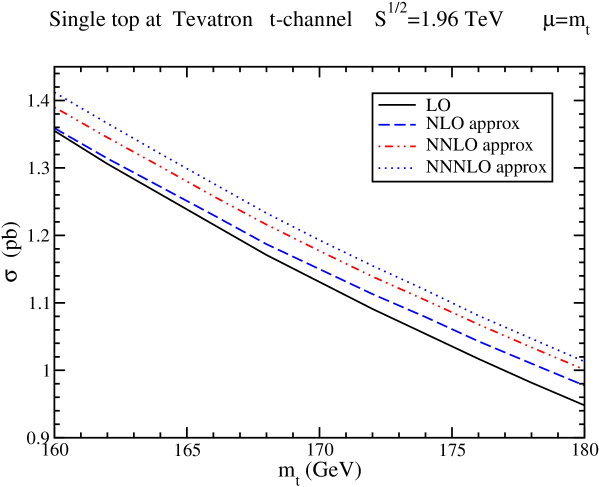
Figure 8: The cross section for single top quark production at the Tevatron in the $t$ channel. Here $\mu=\mu_{F}=\mu_{R}=m_{t}$.

The relative contribution from higher orders is shown in Fig. 9 where the $K$ factors, defined as ratios of the higher-order cross sections to LO, are shown. The $K$ factors in the $t$ channel are small, showing that the corrections do not provide a big enhancement to the cross section.

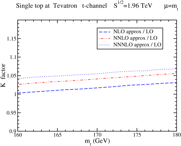
Figure 9: The $K$ factors for single top quark production at the Tevatron in the $t$ channel. Here $\mu=\mu_{F}=\mu_{R}=m_{t}$.

In Fig. 10 we plot the scale dependence of the cross section with $m_{t}=175$ GeV. We set the factorization scale equal to the renormalization scale and vary this common scale $\mu$ over two orders of magnitude. We show results for the LO and higher-order cross sections.

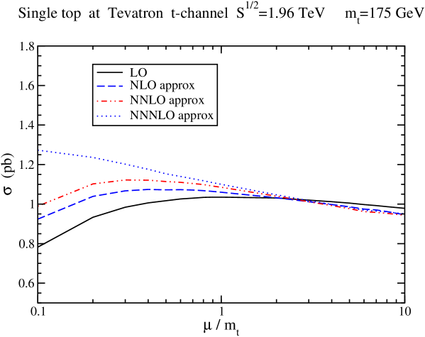
Figure 10: Scale dependence of the single top quark cross section at the Tevatron in the $t$ channel. Here $\mu=\mu_{F}=\mu_{R}$.

In general the factorization and renormalization scales are independent and it is interesting to see the dependence of the cross section separately on each scale. In Fig. 11 we plot the factorization scale, $\mu_{F}$, dependence of the cross section, while setting the renormalization scale $\mu_{R}=m_{t}$. We vary $\mu_{F}$ over two orders of magnitude. At LO the result is exactly the same as in Fig. 10 because at LO there is no $\mu_{R}$ dependence. However at higher orders the difference is noticable.

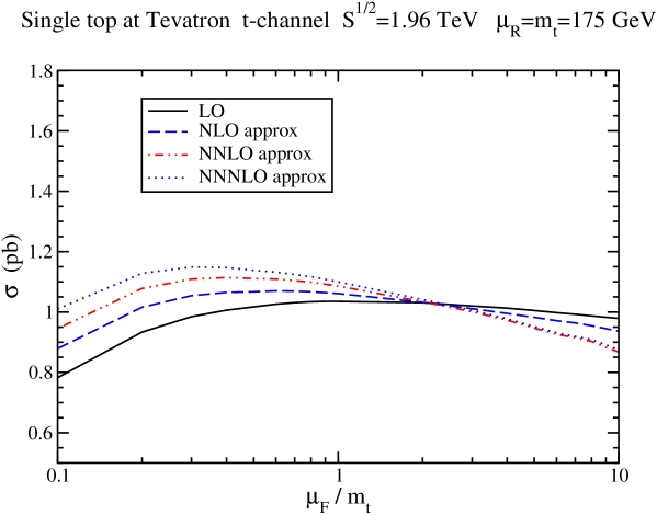
Figure 11: Factorization scale dependence of the single top quark cross section at the Tevatron in the $t$ channel. Here the renormalization scale is held fixed, $\mu_{R}=m_{t}=175$ GeV.

In Fig. 12 we plot the renormalization scale, $\mu_{R}$, dependence of the cross section, while setting the factorization scale $\mu_{F}=m_{t}$. We vary $\mu_{R}$ over two orders of magnitude. At LO the result is exactly flat because, as noted above, at LO there is no $\mu_{R}$ dependence. At higher orders there is a $\mu_{R}$ dependence, though it is fairly flat compared to the $\mu_{F}$ dependence in Fig. 11.

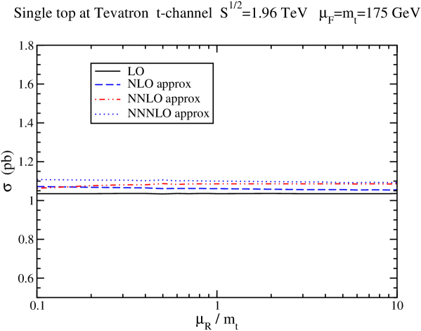
Figure 12: Renormalization scale dependence of the single top quark cross section at the Tevatron in the $t$ channel. Here the factorization scale is held fixed, $\mu_{F}=m_{t}=175$ GeV.

5 Single top quark production via the $s$ channel at the Tevatron

We continue with the $s$ channel. The dominant process (with percentage contribution to the cross section) is $u{\bar{d}}\rightarrow{\bar{b}}t$ (97.4%). Additional processes are $c{\bar{s}}\rightarrow{\bar{b}}t$ (1.1%) and the Cabibbo-suppressed $u{\bar{s}}\rightarrow{\bar{b}}t$ (1.1%), $c{\bar{d}}\rightarrow{\bar{b}}t$ (0.26%), and $u{\bar{d}}\rightarrow{\bar{s}}t$ (0.17%); the contributions from even more suppressed processes ($u{\bar{d}}\rightarrow{\bar{d}}t$, $c{\bar{s}}\rightarrow{\bar{d}}t$, etc.) are negligible.

$s$ channel	LO	NLO approx	NNLO approx	NNNLO approx
$m_{t}=170$	0.353	0.510	0.555	0.576
$m_{t}=172$	0.335	0.484	0.528	0.547
$m_{t}=175$	0.310	0.448	0.488	0.506

Table 2: The leading-order and approximate higher-order cross sections for top quark production in the $s$ channel in pb for $p\overline{p}$ collisions with $\sqrt{S}=1.96$ TeV and $m_{t}=170$, 172, and 175 GeV. We use the MRST2004 NNLO pdf and we set $\mu_{F}=\mu_{R}=m_{t}$.

In Table 2 we give results for the LO cross section and for the approximate NLO, NNLO, and NNNLO cross sections with the threshold corrections at NLL accuracy. The soft-gluon corrections are relatively large for this channel, in stark contrast with the results we found in the $t$ channel. This is also true for the exact NLO cross section [15]. That the behavior of the two channels is quite different should not be surprising: the kinematics and the color flows are quite different. The $t$ channel resembles deep inelastic scattering while the $s$ channel resembles the Drell-Yan process. As we will see, there are differences between the channels not only in the $K$ factors but also in the scale dependence. We also note that the approximate NLO cross section in the $s$ channel is only 3% larger than the exact NLO result, showing that the threshold corrections are dominant and provide the bulk of the QCD corrections and, thus, that the threshold approximation works very well.

Again, it is interesting to provide the cross section for the specific value of the new mass from the Tevatron, $m_{t}=171.4\pm 2.1$ GeV. The NNNLO approximate cross section at 171.4 GeV is 0.555 pb. If we match this to the exact NLO cross section, then the matched cross section (i.e. exact NLO plus NNLO and NNNLO threshold corrections) is

$$\sigma^{s-{\rm channel}}(m_{t}=171.4\pm 2.1\,{\rm GeV})=0.54\pm 0.02\pm 0.03\,\pm 0.01\;{\rm pb}\,,$$ (5.1)

where the first uncertainty is due to scale variation between $m_{t}/2$ and $2m_{t}$, the second is due to the mass ($\pm 2.1$ GeV), and the third is the pdf uncertainty, as discussed in the previous section. Adding these uncertainties in quadrature we find that $\sigma^{s-{\rm channel}}(m_{t}=171.4\pm 2.1\,{\rm GeV})=0.54\pm 0.04$ pb.

As before, it is also important to provide the matched cross section for $m_{t}=175$ GeV. As shown in Table 2, the NNNLO approximate cross section at 175 GeV is 0.506 pb. After matching to the exact NLO cross section we find $\sigma^{s-{\rm channel}}(m_{t}=175\,{\rm GeV})=0.49\pm 0.02\pm 0.01$ pb, where the first uncertainty is due to the scale dependence and the second is due to the pdf, and no uncertainty is considered for the mass. Adding these uncertainties in quadrature we find $\sigma^{s-{\rm channel}}(m_{t}=175\,{\rm GeV})=0.49\pm 0.02$ pb.

In Fig. 13 we plot the cross section for single top quark production at the Tevatron with $\sqrt{S}=1.96$ TeV in the $s$ channel using the MRST2004 parton densities and setting both the factorization and renormalization scales to $\mu=m_{t}$. We plot the LO cross section and the approximate NLO, NNLO, and NNNLO cross sections at NLL accuracy.

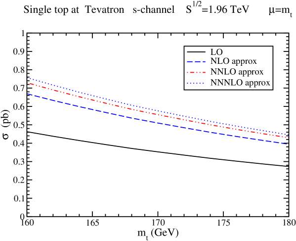
Figure 13: The cross section for single top quark production at the Tevatron in the $s$ channel. Here $\mu=\mu_{F}=\mu_{R}=m_{t}$.

The $K$ factors are shown in Fig. 14. They are quite large, thus showing that the corrections provide a big enhancement to the cross section. This behavior is to be contrasted with the $t$ channel where the corrections are small. We also note that the $K$-factors in the $s$ channel are fairly constant over the top-quark mass range shown. As seen in the plot, the NLO corrections provide a 45% increase of the LO cross section, the NNLO corrections provide an additional 12%, and the NNNLO corrections a further 6%.

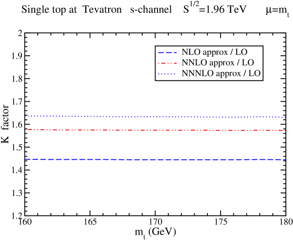
Figure 14: The $K$ factors for single top quark production at the Tevatron in the $s$ channel. Here $\mu=\mu_{F}=\mu_{R}=m_{t}$.

In Fig. 15 we plot the scale dependence of the cross section with $m_{t}=175$ GeV. We set the factorization scale equal to the renormalization scale and vary this common scale $\mu$ over two orders of magnitude. We show results for the LO and higher-order cross sections.

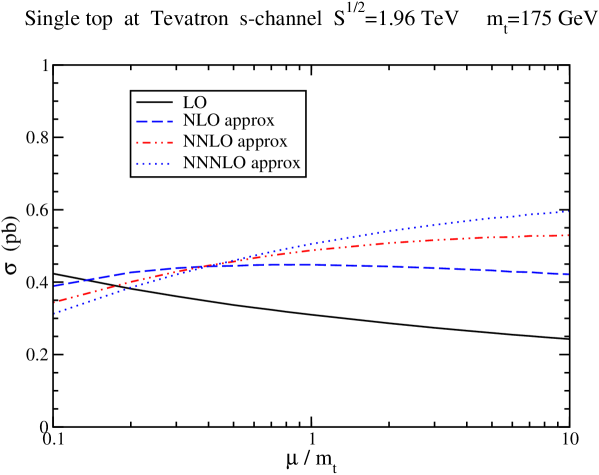
Figure 15: Scale dependence of the single top quark cross section at the Tevatron in the $s$ channel. Here $\mu=\mu_{F}=\mu_{R}$.

Again, we note that the factorization and renormalization scales are theoretically independent, and it is interesting to see the dependence of the cross section separately on each scale. In Fig. 16 we plot the factorization scale, $\mu_{F}$, dependence of the cross section, while setting the renormalization scale $\mu_{R}=m_{t}$. We vary $\mu_{F}$ over two orders of magnitude. At LO the result is exactly the same as in Fig. 15 because of the lack of $\mu_{R}$ dependence.

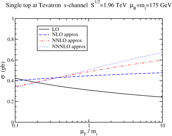
Figure 16: Factorization scale dependence of the single top quark cross section at the Tevatron in the $s$ channel. Here the renormalization scale is held fixed, $\mu_{R}=m_{t}=175$ GeV.

In Fig. 17 we plot the renormalization scale, $\mu_{R}$, dependence of the cross section, while setting the factorization scale $\mu_{F}=m_{t}$. We vary $\mu_{R}$ over two orders of magnitude. At LO the result is exactly flat, as noted before. At higher orders there is a $\mu_{R}$ dependence and it is less flat than for the $t$ channel.

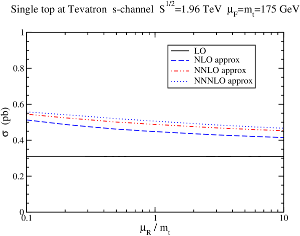
Figure 17: Renormalization scale dependence of the single top quark cross section at the Tevatron in the $s$ channel. Here the factorization scale is held fixed, $\mu_{F}=m_{t}=175$ GeV.

6 Associated $tW$ production at the Tevatron

Associated $tW$ production proceeds via $bg\rightarrow tW^{-}$ (Cabibbo-suppressed contributions from $sg\rightarrow tW^{-}$ and $dg\rightarrow tW^{-}$ are negligible). The kinematics and color flow for this process are rather different from both the $t$ and $s$ channels since we have a real $W$ boson in the final state and a quark-gluon vertex at lowest order.

The LO cross section is 0.070 pb for $m_{t}=175$ GeV, which is a rather small cross section and thus makes this channel relatively unimportant at the Tevatron even after we have added the threshold corrections.

$tW$ production	LO	NLO approx	NNLO approx	NNNLO approx
$m_{t}=170$	0.080	0.122	0.140	0.146
$m_{t}=172$	0.076	0.116	0.133	0.139
$m_{t}=175$	0.070	0.107	0.122	0.127

Table 3: The leading-order and approximate higher-order cross sections for associated $tW$ production in pb for $p\overline{p}$ collisions with $\sqrt{S}=1.96$ TeV and $m_{t}=170$, 172, and 175 GeV. We use the MRST2004 NNLO pdf and we set $\mu_{F}=\mu_{R}=m_{t}$.

In Table 3 we give results for the LO and the approximate NLO, NNLO, and NNNLO cross sections that include the threshold corrections at NLL accuracy at each order. The soft-gluon corrections are relatively large for this channel, even more than in the $s$ channel.

Again, it is interesting to give a result for the specific value of the new mass from the Tevatron, $m_{t}=171.4\pm 2.1$ GeV. The NNNLO approximate cross section at 171.4 GeV is

$$\sigma^{tW}(m_{t}=171.4\pm 2.1\,{\rm GeV})=0.14\pm 0.02^{+0.01}_{-0.02}\,\pm 0.02\;{\rm pb}\,,$$ (6.1)

where the first uncertainty is due to scale variation between $m_{t}/2$ and $2m_{t}$, the second is due to the mass ($\pm 2.1$ GeV), and the third is the pdf uncertainty, as discussed previously. Adding these uncertainties in quadrature we find that $\sigma^{tW}(m_{t}=171.4\pm 2.1\,{\rm GeV})=0.14\pm 0.03$ pb. We note that since an exact NLO result is not available we do not provide a matched cross section here.

As before, it is also important to provide the cross section for $m_{t}=175$ GeV. As shown in Table 3, the NNNLO approximate cross section at 175 GeV is 0.127 pb. Including uncertainties we have $\sigma^{tW}(m_{t}=175\,{\rm GeV})=0.13\pm 0.02\pm 0.02$ pb, where the first uncertainty is due to the scale dependence and the second is due to the pdf, and no uncertainty is considered for the mass. Adding these uncertainties in quadrature we find $\sigma^{tW}(m_{t}=175\,{\rm GeV})=0.13\pm 0.03$ pb.

In Fig. 18 we plot the cross section for single top production at the Tevatron with $\sqrt{S}=1.96$ TeV via associated $tW$ production using the MRST2004 parton densities and setting both the factorization and renormalization scales to $\mu=m_{t}$. We plot the LO cross section and the approximate NLO, NNLO, and NNNLO cross sections at NLL accuracy.

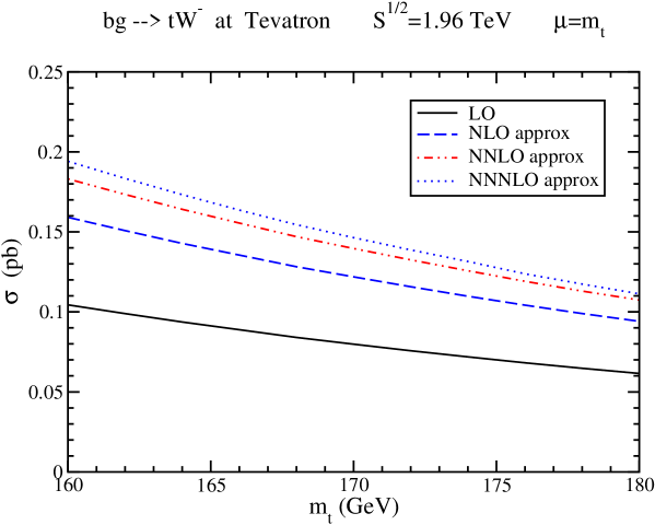
Figure 18: The cross section for associated $tW$ production at the Tevatron. Here $\mu=\mu_{F}=\mu_{R}=m_{t}$.

The relative contribution from higher orders is shown in Fig. 19. The $K$ factors are quite large, showing that the soft-gluon corrections provide a big enhancement to the cross section, and fairly constant over the top-quark mass range shown. As seen from the plot, the NLO corrections provide a 53% increase of the LO cross section, the NNLO corrections provide an additional 22%, and the NNNLO corrections a further 8%. However, the overall cross section still remains rather small and we will not study it further here.

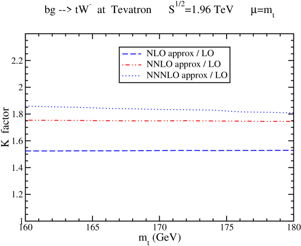
Figure 19: The $K$ factors for associated $tW$ production at the Tevatron. Here $\mu=\mu_{F}=\mu_{R}=m_{t}$.

7 Conclusion

We have studied single top quark production at the Tevatron via all Standard Model partonic processes. We have presented the resummation of the threshold soft-gluon corrections and their expansion to provide higher-order approximate cross sections through NNNLO.

The results differ a lot among channels. In the $t$ channel the soft-gluon corrections are small and hence do not greatly change the LO result. Including soft gluon corrections through NNNLO at NLL accuracy and matching with the exact NLO cross section, our best estimate of the cross section is $\sigma^{t-{\rm channel}}(m_{t}=171.4\pm 2.1\,{\rm GeV})=1.15\pm 0.07$ pb, where the uncertainty indicated includes the scale dependence, the uncertainty in the top quark mass, and the pdf uncertainty.

In the $s$ channel, however, the corrections are significant. The NLO approximate cross section is an excellent approximation to the full NLO result, thus showing that the threshold approximation works very well, while the higher-order contributions provide further enhancements. Our best estimate for the cross section in this channel is $\sigma^{s-{\rm channel}}(m_{t}=171.4\pm 2.1\,{\rm GeV})=0.54\pm 0.04$ pb.

The renormalization and factorization scale dependence of the cross section for both $t$ and $s$ channels were displayed both separately and also setting the scales equal to each other.

The threshold corrections for associated $tW$ production are large as a percentage of the LO cross section (large $K$ factors), however even with those the total cross section is still rather small for this channel. We find $\sigma^{tW}(m_{t}=171.4\pm 2.1\,{\rm GeV})=0.14\pm 0.03$ pb.

Finally, we note that the corresponding cross sections for single antitop quark production at the Tevatron are identical to those for single top quark production as presented in this paper.

Appendix

Here we provide some details on the kinematics of the calculation. We consider the process $p_{1}+p_{2}\rightarrow p_{3}+p_{4}$, where the particles have been represented by their momenta $p_{i}$. If $p_{1}$ and $p_{2}$ refer to incoming partons (quarks or gluons) then $m_{1}=0$ and $m_{2}=0$. The partonic kinematical invariants are $s=(p_{1}+p_{2})^{2}$, $t=(p_{1}-p_{3})^{2}$, $u=(p_{2}-p_{3})^{2}$, $s_{4}=s+t+u-m_{3}^{2}-m_{4}^{2}$. The hadronic kinematical invariants are $S=(p_{h1}+p_{h2})^{2}$, $T=(p_{h1}-p_{3})^{2}$, $U=(p_{h2}-p_{3})^{2}$, $S_{4}=S+T+U-m_{3}^{2}-m_{4}^{2}$, where $h_{1}$ and $h_{2}$ are the hadrons (protons and antiprotons at the Tevatron) corresponding to partons $p_{1}$ and $p_{2}$; thus, $p_{1}=x_{1}p_{h1}$ and $p_{2}=x_{2}p_{h2}$. The relations between partonic and hadronic quantities are as follows: $s=x_{1}x_{2}S$, $t-m_{3}^{2}=x_{1}(T-m_{3}^{2})$, $u-m_{3}^{2}=x_{2}(U-m_{3}^{2})$. Then

$$\frac{S_{4}}{S} = \frac{s_{4}}{s}-(1-x_{1})\frac{(u-m_{4}^{2})}{s}-(1-x_{2})\frac{(t-m_{4}^{2})}{s}+{\cal O}((1-x_{1})(1-x_{2}))\,.$$ (A.1)

If we denote by $\sigma$ the hadron-level cross section and by ${\hat{\sigma}}$ the parton-level cross section, then we have the relations

$$\sigma = \int dx_{1}\,dx_{2}\,\phi(x_{1})\,\phi(x_{2})\,{\hat{\sigma}}$$

$$\Rightarrow\frac{d\sigma}{dT\,dU} = \int dx_{1}\,dx_{2}\,\frac{dt}{dT}\,\frac{du}{dU}\,\phi(x_{1})\,\phi(x_{2})\,\frac{d{\hat{\sigma}}}{dt\,du}$$ (A.2)

where $\phi(x)$ are the parton distributions. Now $dt=x_{1}dT$ and $du=x_{2}dU$, so

$$\frac{d\sigma}{dT\,dU} = \int dx_{1}\,dx_{2}\,x_{1}\,x_{2}\,\phi(x_{1})\,\phi(x_{2})\,\frac{d{\hat{\sigma}}}{dt\,du}$$

$$\Rightarrow\sigma = \int dT\,dU\,dx_{2}\,ds_{4}\,\frac{x_{1}x_{2}}{x_{2}S+T-m_{3}^{2}}\,\phi(x_{1})\,\phi(x_{2})\,\frac{d{\hat{\sigma}}}{dt\,du}\,,$$ (A.3)

where we used the relation

$$x_{1}=\frac{s_{4}-m_{3}^{2}+m_{4}^{2}-x_{2}(U-m_{3}^{2})}{x_{2}S+T-m_{3}^{2}}\,.$$ (A.4)

Writing explicitly the kinematical limits on the integrals, we get the precise expression for the hadronic cross section

$$\sigma_{p_{h1}p_{h2}\rightarrow p_{3}p_{4}}(S) = \int_{T_{min}}^{T_{max}}dT\int_{U_{min}}^{U_{max}}dU\int_{x_{2min}}^{1}dx_{2}\int_{0}^{s_{4max}}ds_{4}$$ (A.5)

$$\times\frac{x_{1}x_{2}}{x_{2}S+T-m_{3}^{2}}\,\phi(x_{1})\,\phi(x_{2})\,\frac{d^{2}{\hat{\sigma}}_{p_{1}p_{2}\rightarrow p_{3}p_{4}}}{dt\,du}$$

where $x_{1}$ is given in Eq. (A.4), and the limits on the integrals are

$$T_{{}^{max}_{min}}=-\frac{1}{2}(S-m_{3}^{2}-m_{4}^{2})\pm\frac{1}{2}\sqrt{(S-m_{3}^{2}-m_{4}^{2})^{2}-4m_{3}^{2}m_{4}^{2}}\,,$$ (A.6)

$$U_{max}=m_{3}^{2}+\frac{m_{3}^{2}S}{T-m_{3}^{2}}\,,\quad U_{min}=-S-T+m_{3}^{2}+m_{4}^{2}\,,$$ (A.7)

$$x_{2min}=\frac{m_{4}^{2}-T}{S+U-m_{3}^{2}}\,,$$ (A.8)

and $s_{4max}=x_{2}(S+U-m_{3}^{2})+T-m_{4}^{2}$.

The Born-level differential partonic cross section is written as

$$\frac{d^{2}{\hat{\sigma}}^{B}_{p_{1}p_{2}\rightarrow p_{3}p_{4}}}{dtdu}=F^{B}_{p_{1}p_{2}\rightarrow p_{3}p_{4}}\delta(s_{4})=\frac{\mid{\cal M}_{p_{1}p_{2}p_{3}p_{4}}\mid^{2}}{16\pi s^{2}}\delta(s_{4})\,,$$ (A.9)

where the amplitude squared has to be specified for the partonic process studied.

For the $t$-channel process $ub\rightarrow dt$ we have

$$|{\cal M}_{ub\rightarrow dt}|^{2}=\frac{4\pi^{2}\alpha^{2}V_{tb}^{2}V_{ud}^{2}}{\sin^{4}\theta_{W}}\frac{s(s-m_{t}^{2})}{(t-m_{W}^{2})^{2}}\,.$$ (A.10)

For the $t$-channel process ${\bar{d}}b\rightarrow{\bar{u}}t$ we have

$$|{\cal M}_{{\bar{d}}b\rightarrow{\bar{u}}t}|^{2}=\frac{4\pi^{2}\alpha^{2}V_{tb}^{2}V_{ud}^{2}}{\sin^{4}\theta_{W}(t-m_{W}^{2})^{2}}\left[(s+t)^{2}-(s+t)m_{t}^{2}\right]\,.$$ (A.11)

For the $s$-channel process $u{\bar{d}}\rightarrow{\bar{b}}t$ we have

$$|{\cal M}_{u{\bar{d}}\rightarrow{\bar{b}}t}|^{2}=\frac{4\pi^{2}\alpha^{2}V_{tb}^{2}V_{ud}^{2}}{\sin^{4}\theta_{W}}\frac{t(t-m_{t}^{2})}{(s-m_{W}^{2})^{2}}\,.$$ (A.12)

For the associated production process $bg\rightarrow tW^{-}$ we have

$$|{\cal M}_{bg\rightarrow tW^{-}}|^{2}=\frac{4\pi^{2}V_{tb}^{2}\alpha_{s}\alpha}{3m_{W}^{2}\sin^{2}\theta_{W}}\left(\frac{A_{1}}{u_{1}^{2}}-\frac{2A_{2}}{u_{1}s}+\frac{2A_{3}}{s^{2}}\right)\,,$$ (A.13)

where $A_{1}=-u_{2}(s-m_{t}^{2}-m_{W}^{2})(m_{W}^{2}+m_{t}^{2}/2)-(t_{1}/2)(-2m_{W}^{4}+m_{W}^{2}m_{t}^{2}+m_{t}^{4})-2u_{2}m_{t}^{2}(2m_{W}^{2}+m_{t}^{2})$, $A_{2}=-t_{1}(-m_{W}^{2}+m_{t}^{2})m_{W}^{2}-(u_{2}/2)t_{1}m_{t}^{2}-u_{1}(u_{2}/2)m_{t}^{2}-sm_{W}^{2}m_{t}^{2}-(s/2)m_{t}^{4}$, $A_{3}=-u_{1}(s/4)(2m_{W}^{2}+m_{t}^{2})$ where $\alpha=e^{2}/(4\pi)$ and $\alpha_{s}$ is the strong coupling.

The expressions for the corresponding processes involving charm quarks and Cabibbo-suppressed contributions are similar.

The electroweak parameters used in the above expressions and throughout the paper are the following [35]:

$m_{W}=80.403$ GeV,

$G_{F}=\frac{g_{W}^{2}}{4\sqrt{2}m_{W}^{2}}=1.16637\times 10^{-5}$ GeV^-2,

$\sin^{2}\theta_{W}|_{Z}=0.23122$,

$e=g_{W}\sin\theta_{W}=0.31404$,

$\alpha=e^{2}/(4\pi)=7.848\times 10^{-3}$.

For the CKM matrix elements we have used [35]

$V_{ud}=0.97383$, $V_{us}=0.2272$, $V_{ub}=0.00396$,

$V_{cd}=0.2271$, $V_{cs}=0.97296$, $V_{cb}=0.04221$,

$V_{td}=0.00814$, $V_{ts}=0.04161$, $V_{tb}=0.9991$.