Pressure of the standard model

Abstract

We review the computation of the thermodynamic pressure of the entire minimal standard model to three loop order, performed in [1].

1 INTRODUCTION

Computing the thermodynamic pressure of the gauge field theories, defined by the path integral

$$p(T)=\lim_{V\rightarrow\infty}\frac{T}{V}\int\mathcal{D}\varphi\,\mathrm{exp}(-S_{\mathrm{Euclidean}}[\varphi]),$$ (1)

has attracted a lot of interest over the years. In addition to being an interesting computation in itself, pressure is a phenomenologically important quantity when trying to understand the properties of quark-gluon plasma produced in heavy-ion collisions (relevant physics being described by QCD) and also in cosmology (see, for example, [2]). In QCD with massless quarks, the expansion of the pressure in terms of the gauge coupling $g$ is known today to the last perturbatively computable term [3]. In the full standard model, the pressure is less well known, the interest having been focused on the properties of the electroweak phase transition (crossover) which depend only on the pressure difference between the phases of the theory. In this talk, we will review our recent computation of the pressure of the full minimal standard model to three loop order, or to order $g^{5}$ in the coupling constants. We will also outline some of the differences arising in the computations of the QCD pressure and the full standard model pressure.

2 FRAMEWORK OF THE COMPUTATION

As well known, straightforward perturbative computations in gauge field theories at high temperatures are inhibited by infrared divergences that require resummation [4]. A convenient way to perform the resummation is to construct effective field theories for the infrared sensitive modes (the bosonic zero modes) by integrating out the infrared safe modes (see [1, 5] for details). In case of the standard model, the resulting effective theory will be a three dimensional gauge field theory with fundamental (Higgs) and adjoint (temporal components of the gauge fields, corresponding to the electrostatic modes of the full theory) scalars, defined by the action

$$S_{\mathrm{E}} = \int\mathrm{d}^{3}x\left(\frac{1}{4}F_{ij}F_{ij}+\frac{1}{4}G^{a}_{ij}G^{a}_{ij}+\frac{1}{2}(D_{i}A_{0}^{a})^{2}+\frac{1}{2}(\partial_{i}B_{0})^{2}+\frac{1}{2}m_{D}^{2}A_{0}^{a}A_{0}^{a}+\frac{1}{2}m_{D}^{\prime 2}B_{0}B_{0}\right.$$ (2)

$$\;\;\;\;\;\;\;\;\;\;\;\left.+|D_{i}\Phi|^{2}+m_{3}^{2}|\Phi|^{2}+\mathcal{L}_{\mathrm{E,int}}(\Phi,A_{0}^{a},B_{0})\right).$$

In this theory, the scalars have obtained thermal masses ($m_{3}^{2}\sim-\nu^{2}+g^{2}T^{2}$ for the Higgs and $m_{D}^{2}\sim m_{D}^{\prime 2}\sim g^{2}T^{2}$ for the adjoint scalars) that serve to regulate (some of) the infrared divergences.

Within this framework, assuming for now that the temperature is well above the temperatures corresponding to the electroweak crossover, the recipe for calculating the pressure is:

• Compute the strict perturbative expansion of the pressure in the full theory, schematically giving us (using dimensional regularization, $d=4-2\epsilon$)

  $$p_{\mathrm{E}}(T)\sim T^{4}\left[1+g^{2}+g^{4}\left(1/\epsilon+1+\ln\Lambda/T\right)+\mathcal{O}(g^{6})\right],$$ (3)

  leaving uncancelled infrared divergences at order $g^{4}$ (three loop order).

• Construct the three dimensional effective theory for the bosonic zero modes and compute its pressure, schematically

  $$p_{\mathrm{M}}(T)/T\sim m^{3}+g_{3}^{2}m^{2}\left(1/\epsilon+1+\ln\Lambda/m\right)+g_{3}^{4}m+\mathcal{O}(g_{3}^{6}).$$ (4)

  Here $m$ refers both to $m_{3}$ and $m_{D}$ and $g_{3}^{2}=g^{2}T$.

The total pressure is then given as the sum of these two contributions, $p(T)=p_{\mathrm{E}}(T)+p_{\mathrm{M}}(T)+\mathcal{O}(g^{6})$. The $1/\epsilon$ poles in $p_{\mathrm{M}}(T)$ exactly cancel those of $p_{\mathrm{E}}(T)$, thus making $p(T)$ infrared finite.

2.1 What happens near the electroweak crossover?

The perturbative expansion of the QCD pressure becomes unreliable at temperatures near $T_{c}$ because confinement effects become important ($\Lambda_{\mathrm{QCD}}\sim T_{c}$). The Landau pole of the electroweak theory, however, corresponds to a length scale comparable to the radius of the Earth and one can therefore expect the confinement effects to be negligible in the electroweak case, enabling us to extend the perturbative computations all the way down to the electroweak crossover.

Near the crossover region the fundamental scalar, which drives the transition, becomes light compared to the adjoint scalars, thus introducing a new mass hierarchy to the system. Consequently, the computation outlined above becomes invalid since it implicitly assumes that both the fundamental and the adjoint scalars can be considered heavy with masses $m\sim gT$. However, since the adjoint scalars are now heavy compared to the fundamental scalar, they can be integrated out leading to a new effective theory describing just the fundamental scalar and the magnetic components of the gauge bosons,

$$S_{\mathrm{E2}}=\int\mathrm{d}^{3}x\left(\frac{1}{4}F_{ij}F_{ij}+\frac{1}{4}G^{a}_{ij}G^{a}_{ij}+|D_{i}\Phi|^{2}+\widetilde{m}_{3}^{2}|\Phi|^{2}+\widetilde{\lambda}|\Phi|^{4}\right),$$ (5)

where $\widetilde{m}_{3}^{2}\sim m_{3}^{2}-g_{3}^{2}m_{D}\ll m_{D}^{2}$ (valid near the crossover). The contribution of the effective theories to the pressure is then divided into two parts: contribution from the adjoint scalars, $p_{\mathrm{M1}}$, and the contribution from the remaining degrees of freedom, $p_{\mathrm{M2}}$. These can be written as $p_{\mathrm{M}}(T)=p_{\mathrm{M1}}(T)+p_{\mathrm{M2}}(T)$, where

$$p_{\mathrm{M1}}/T \sim m_{D}^{3}+g_{3}^{2}m_{D}^{2}\left(1/\epsilon+1+\ln\Lambda/T\right)+g_{3}^{4}m_{D}\left(1/\epsilon+1+\ln\Lambda/T\right)+\mathcal{O}(g_{3}^{6}),$$ (6)

$$p_{\mathrm{M2}}/T \sim \widetilde{m}_{3}^{3}+\widetilde{g}_{3}^{2}\widetilde{m}_{3}^{2}\left(1/\epsilon+1+\ln\Lambda/\widetilde{m}_{3}\right)+\mathcal{O}(\widetilde{g}_{3}^{4}\widetilde{m}_{3}).$$ (7)

Since the fundamental scalar becomes light near the crossover, new infrared divergences (terms $\sim g_{3}^{4}m_{D}/\epsilon$) appear that cancel only when the contribution from the second effective theory $S_{\mathrm{E2}}$ is taken into account. It is noteworthy that the new poles appear at order $g^{5}$, thus leading to terms of the order of $g^{5}\ln g$ in the expansion of the full pressure. Such terms are not present in the expansion of the QCD pressure.

3 NUMERICAL RESULTS

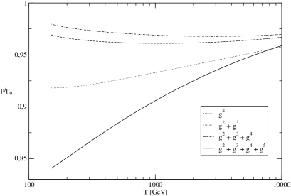
Figure 1: The expansion of the pressure of the minimal standard model to various orders in $g^{2}$.

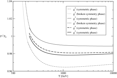
Figure 2: The expansion of the pressure of the SU(2) + Higgs theory to various orders in $g^{2}$.

The detailed analytic expression of the expansion of the pressure is given in [1] and we will here content to reviewing some numerical results obtained from that. In Fig. 2 we have plotted the expansion at different orders in $g^{2}$, normalized to the pressure of ideal gas of massless particles $p_{0}(T)=106.75\cdot\pi^{2}T^{4}/90$. The result deviates strongly from the ideal gas result, up to as much as 15%. As discussed in [2], such a departure from the ideal gas result may affect the predictions concerning the WIMP relic density in the universe.

As can also be seen from the plot, the expansion does not converge well; the order $g^{5}$ term produces a significant correction to the pressure compared to the previous terms. The poor convergence is mostly due to the QCD contributions (of the 106.75 bosonic degrees of freedom in the standard model, 79 come from QCD). To analyze the convergence within the electroweak sector, we can study a simpler SU(2) + Higgs theory. As can be seen from the plot in Fig. 2, also normalized to the ideal gas pressure, the expansion within just the electroweak sector converges better: each new term in the expansion is smaller than the previous one. Similar conclusions can be reached by studying the scale dependence of the expansion.

As we approach the crossover region, the high temperature computation ceases to be valid as discussed in the previous section. This can be explicitly seen in Fig. 3. The high temperature expansion of the pressure (denoted by $p_{\mathrm{HT}}(T)$ in the plot) contains an unphysical singularity due to the infrared divergences which appear when $m_{3}\rightarrow 0$. Taking into account that the Higgs scalar becomes light near the crossover, the expansion behaves well all the way down to the electroweak crossover ($p_{\mathrm{PT}}(T)$). This result can therefore be used for a precise determination of the expansion rate of the universe near the electroweak crossover, which is important in many cosmological studies.

This work has been done in collaboration with M. Vepsäläinen.

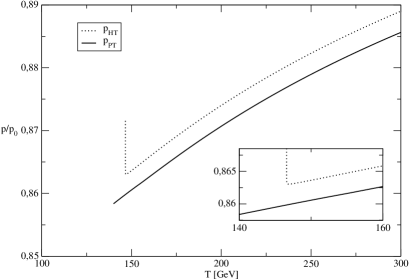
Figure 3: The pressure near the electroweak crossover according to the high temperature computation ($p_{\mathrm{HT}}(T)$) and the computation taking into account that the fundamental scalar is light near the crossover.

References

- [1] A. Gynther and M. Vepsäläinen, JHEP 0601, 060 (2006), [hep-ph/0510375]. JHEP 0603, 011 (2006), [hep-ph/0512177].
- [2] M. Hindmarsh and O. Philipsen, Phys. Rev. D 71, 087302 (2005), [hep-ph/0501232].
- [3] K. Kajantie, M. Laine, K. Rummukainen and Y. Schröder, Phys. Rev. D 67, 105008 (2003), [hep-ph/0211321]. A. Vuorinen, Phys. Rev. D 68, 054017 (2003), [hep-ph/0305183].
- [4] A. D. Linde, Phys. Lett. B 96, 289 (1980)
- [5] K. Kajantie, M. Laine, K. Rummukainen and M. E. Shaposhnikov, Nucl. Phys. B 458, 90 (1996), [hep-ph/9508379].