New constraints on R-parity violating couplings through the measurements of the $B^{0}_{s(d)}$-${\bar{B}^{0}_{s(d)}}$ and $K^{0}$-$\bar{K}^{0}$ mixing

Abstract

We calculate contributions to $B_{s}-\bar{B}_{s}$ mixing through tree-level sneutrino exchange in the framework of the minimal supersymmetric standard model with R-parity violation, including the next-to-leading-order QCD corrections. We compare our results with the updated bounds on the $B_{s}-\bar{B}_{s}$ mass difference reported by CDF collaborations, and present new constraints on the relevant combinations of parameters of the minimal supersymmetric standard model with R-parity violation. Our results show that upper bound on the relevant combination of couplings of $B_{s}-\bar{B}_{s}$ mixing is of the order $10^{-9}$. We also calculate the $B^{0}_{d}-\bar{B}^{0}_{d}$ and $K^{0}-\bar{K}^{0}$ mass differences, and show that the upper bounds on the relevant combinations of couplings are two and four orders of magnitude stronger than ones reported in the literatures, respectively. We also discuss the case of complex couplings and show that how the relevant combinations of couplings are constrained by the updated experiment data of $B_{s}-\bar{B}_{s}$, $B_{d}-\bar{B}_{d}$ mixing and time-dependent CP asymmetry $S_{J/\psi K_{s}}$, and future possible observations of $S_{J/\psi\phi}$ at LHCb, respectively.

I introduction

Very recently, the DØ collaboration and the CDF collaboration at the Fermilab Tevatron reported their updated measurements of the mass difference between $B_{s}$ and $\bar{B}_{s}$ mesons ($\Delta m_{s}$). The new bounds on the mass difference are exp1 ; exp2 :

$$\text{D\O:}\quad 17~{}\text{ps}^{-1}<\Delta m_{s}<21~{}\text{ps}^{-1}$$

$$\text{CDF:}\quad\Delta m_{s}=17.77^{+0.10}_{-0.10}\pm 0.07~{}\text{ps}^{-1}$$ (1)

It was the first time that both the lower bound and the upper bound for the $B_{s}-\bar{B}_{s}$ mixing are presented. Especially the CDF result has reached an accuracy of about 1%. The new results are important for the precision test of the standard model (SM), especially for the determination of the unitary triangle. Moreover, if the SM predictions are consistent with the above results, these data will put severe constraints on the flavor structure of the possible new physics models beyond the SM.

In the literature, there have already been many discussions about the implications of the new measurements. In Ref. buras2 ; Ligeti:2006pm ; Ball:2006xx ; Alakabha Datta ; UTfit , the authors carried out model-independent analysis of the constraints on extensions of the SM. There are also model-dependent calculations in some new physics models beyond the SM FVMSSM ; LHM ; Zprime ; Zprime2 ; GUT ; Paradisi ; Jonparry . In this paper, we further investigate the effects of the minimal supersymmetric standard model with R-parity violation (MSSM-RPV) RPV on the neutral meson mixing.

R-parity is a discrete symmetry defined by $R_{p}=(-1)^{3B+L+2S}$, where B is the baryon number,L is the lepton number and S is the spin of the particle. In a supersymmetric extension of the SM, all the particles in the SM have $R_{p}=1$, while all the superpartners have $R_{p}=-1$. R-parity conservation is imposed in the minimal supersymmetric standard model (MSSM) to keep proton stable. However, this requirement is not necessary for a fundamental theory, and one can always introduce lepton number or baryon number violating terms in the Lagrangian. For the neutral meson mixing, the relevant terms in the Lagrangian are

$$\mathcal{L}_{\text{RPV}}=\lambda^{\prime}_{ijk}\tilde{\nu}_{iL}\bar{d}_{kR}d_{jL}+h.c.$$ (2)

These interaction terms can induce $B_{s}-\bar{B}_{s}$ mixing through tree level sneutrino exchange, and thus, probably, the relevant combination of couplings $\sum\limits_{i}\lambda^{\prime}_{i32}\lambda^{\prime*}_{i23}$ will be severely constrained by the recent measurementsexp1 ; exp2 . Similarly, the terms shown in Eq. (2) also can induce the $B^{0}_{d}-\bar{B}^{0}_{d}$ and $K^{0}-\bar{K}^{0}$ mixing, which were discussed in Ref. Rparity1 at the leading-order, and the constraints on the relevant combinations of couplings through comparing with data were given by Rparity1

$$\sum_{i}\lambda^{\prime}_{i31}\lambda^{\prime*}_{i13}n_{i}\lesssim 3.3\times 10^{-8},$$

$$\sum_{i}\lambda^{\prime}_{i21}\lambda^{\prime*}_{i12}n_{i}\lesssim 4.5\times 10^{-9},$$ (3)

where $n_{i}\equiv(100~{}\text{GeV}/{m_{\tilde{\nu}_{iL}}})^{2}$, $m_{\tilde{\nu}_{iL}}$ is the mass of the sneutrino of the $i$-th generation. However, authors of Ref. Rparity1 did not include the contributions of the SM, since they believed that both theoretical and experimental results involved considerable uncertainties at that time. Recently, both SM theoretical predictions and experimental results has been improved significantly B0andK . Thus, besides investigating of $B^{0}_{s}$-${\bar{B}^{0}_{s}}$ mixing, it is also worthwhile to reinvestigate the constraints on the combinations of R-parity violating (RPV) couplings with the updated data on $B^{0}_{d}$-${\bar{B}^{0}_{d}}$ and $K^{0}$-$\bar{K}^{0}$ mixing including the SM contributions. Moreover, in general, the next-to-leading-order (NLO) QCD corrections are significant, so we also calculate the NLO QCD effects on the above neutral meson mixing in this paper.

In addition to the above mass differences, the R-parity violating couplings can also contribute to the CP asymmetries in the meson decay processes, when the couplings are complex. So the combinations of RPV couplings discussed above can affect observables related to time-dependent CP violation in processes such as $B_{d}\to J/\psi K_{s}$ and $B_{s}\to J/\psi\phi$. In this paper, we also consider the constraints on the relevant combinations of MSSM-RPV couplings from these CP violation observables.

We organize our paper as following. Section II is a brief summary of the formalism for the calculation of the neutral meson mixing , CP asymmetry in B physics and the results in the SM. In Section III , we calculate the contributions from the MSSM-RPV at leading-order and next-to-leading-order in QCD. In section IV, we present our numerical results and discussions.

II Basic formalism and analytical results in the SM

In order to make our paper self-contained, we first illustrate the basic formalism for the calculation of the $B^{0}_{s(d)}$-$\bar{B}^{0}_{s(d)}$ and $K^{0}$-$\bar{K}^{0}$ mass differences $\Delta m$, the time-dependent CP asymmetry in $B_{d}$ decay, $S_{J/\psi K_{s}}$ and the time-dependent CP asymmetry in $B_{s}$ decay, $S_{J/\psi\phi}$.

We start from the $\Delta{F}=2$ effective Hamiltonian buras1

$$\mathcal{H}_{\text{eff}}=\sum_{i}C_{i}Q_{i}+h.c..$$ (4)

The relevant operators for our concerning are

$$Q_{0} =\bar{q}^{\alpha}\gamma_{\mu}P_{L}b^{\alpha}\bar{q}^{\beta}\gamma_{\mu}P_{L}b^{\beta},$$ (5)

$$Q_{1} =\bar{q}^{\alpha}P_{L}b^{\alpha}\bar{q}^{\beta}P_{R}b^{\beta},$$ (6)

$$Q_{2} =\bar{q}^{\alpha}P_{L}b^{\beta}\bar{q}^{\beta}P_{R}b^{\alpha},$$ (7)

where $q=d,s$ for $B_{d}$ or $B_{s}$ meson mixing, respectively. Similar expressions for $K^{0}-\bar{K}^{0}$ mixing can be obtained by replacing $b$ with $s$ and setting $q=d$.

With this effective Hamiltonian, the $B_{q}-\bar{B}_{q}$ mass difference can be expressed as

$$\Delta m_{q}=2\left|\bra{\bar{B}_{q}}\mathcal{H}_{\text{eff}}\ket{B_{q}}\right|=2\left|\sum_{i}C_{i}\bra{\bar{B}_{q}}Q_{i}\ket{B_{q}}\right|;$$ (8)

$a_{J/\psi K_{s}(\phi)}$, time-dependent CP asymmetry in $B_{d(s)}\rightarrow J/\psi K_{s}(\phi)$ decays, can be expressed as

$$a_{J/\psi K_{s}(\phi)}=S_{J/\psi K_{s}(\phi)}\text{sin}\Delta m_{d(s)}t,$$ (9)

where $S_{J/\psi K_{s}(\phi)}=\text{sin}2\beta_{eff}$, and $\beta_{eff}=\frac{1}{2}\text{arg}\bra{\bar{B}_{d(s)}}\mathcal{H}_{\text{eff}}\ket{B_{d(s)}}$. In the framework of SM,

$$S^{SM}_{J/\psi K_{s}}=\text{sin}2\beta,~{}~{}S^{SM}_{J/\psi\phi}=\text{sin}2\beta_{s},$$ (10)

with

$$\beta=\text{arg}(-\frac{(V_{CKM})_{cd}(V_{CKM}^{\ast})_{cb}}{(V_{CKM})_{td}(V_{CKM}^{\ast})_{tb}}),$$

$$\beta_{s}=\text{arg}(-\frac{(V_{CKM})_{ts}(V_{CKM}^{\ast})_{tb}}{(V_{CKM})_{cs}(V_{CKM}^{\ast})_{cb}}).$$ (11)

In the SM, only $C_{0}$ is nonzero, which has been calculated to the NLO in QCD NLOQCDSM ; buras1 and is given by

$$C_{0}(\mu)=\frac{G_{F}^{2}m_{W}^{2}}{4\pi^{2}}(V^{*}_{tb}V_{tq})^{2}\eta_{B}S_{0}(x_{t})\left(\alpha_{s}^{(5)}(\mu)\right)^{-6/23}\left[1+\frac{\alpha_{s}^{(5)}(\mu)}{4\pi}J_{5}\right],$$ (12)

where $\eta_{B}=0.55\pm 0.1$ etaparameter , $J_{5}=1.627$ in the naive dimensional regularization scheme (NDR), $x_{t}=m_{t}^{2}/m_{W}^{2}$ and $S_{0}(x_{t})$ is the Inami-Lim function Inami-Lim . The scale $\mu$ is usually taken to be $\sim m_{b}$ in $B$ physics.

The expression for the $K^{0}-\bar{K}^{0}$ mass difference is a little different, which is given by

$$\Delta m_{K}=2\mathrm{Re}\bra{\bar{K}^{0}}\mathcal{H}_{\text{eff}}\ket{K^{0}}=2\mathrm{Re}\sum_{i}C_{i}\bra{\bar{K}^{0}}Q_{i}\ket{K^{0}}.$$ (13)

The nonzero NLO Wilson coefficient in the SM is

$$C_{0}(\mu)=\frac{G_{F}^{2}m_{W}^{2}}{4\pi^{2}}\left[\lambda_{c}^{2}\eta_{1}S_{0}(x_{c})+\lambda_{t}^{2}\eta_{2}S_{0}(x_{t})+2\lambda_{c}\lambda_{t}\eta_{3}S_{0}(x_{c},x_{t})\right]\left(\alpha_{s}^{(3)}(\mu)\right)^{-2/9}\left[1+\frac{\alpha_{s}^{(3)}(\mu)}{4\pi}J_{3}\right],$$ (14)

where $\lambda_{i}=V^{*}_{is}V_{id}$, $J_{3}=1.895$ in the NDR scheme and the parameters $\eta_{i}$ are $\eta_{1}=1.38\pm 0.20$, $\eta_{2}=0.57\pm 0.01$, $\eta_{3}=0.47\pm 0.04$ etaofK ; etaparameter , respectively. $S_{0}$ functions can be found in Ref.buras1 .

The matrix elements of the operators $Q_{i}$ (i=0,1,2) between two hadronic states can be obtained by using the vacuum insertion approximation (VIA) and partial axial current conservation (PCAC). We refer the readers to Ref. CP-violation for details. The results are

$$\braket{Q_{0}(\mu)} \equiv\bra{\bar{B}_{s}}Q_{0}(\mu)\ket{B_{s}}=\frac{1}{3}f_{B_{s}}^{2}m_{B_{s}}B_{0}(\mu),$$ (15)

$$\braket{Q_{1}(\mu)} \equiv\bra{\bar{B}_{s}}Q_{1}(\mu)\ket{B_{s}}=f_{B_{s}}^{2}m_{B_{s}}\left(\frac{1}{24}-\frac{m_{B_{s}}^{2}}{4(m_{s}(\mu)+m_{b}(\mu))^{2}}\right)B_{1}(\mu),$$ (16)

$$\braket{Q_{2}(\mu)} \equiv\bra{\bar{B}_{s}}Q_{2}(\mu)\ket{B_{s}}=f_{B_{s}}^{2}m_{B_{s}}\left(\frac{1}{8}-\frac{m_{B_{s}}^{2}}{12(m_{s}(\mu)+m_{b}(\mu))^{2}}\right)B_{2}(\mu),$$ (17)

where $m_{B_{s}}$ and $f_{B_{s}}$ is the mass and decay constant of the $B_{s}$ mesons, respectively. Clearly, the expressions for $B_{d}$ and $K^{0}$ mesons can be obtained by simple substitutions. $B_{i}(\mu)$ is the non-perturbative parameters and can be calculated with lattice method KBparameter ; latticeB . We list their values to be used in our numerical calculations in table 1:

	$B_{0}(\mu)$	$B_{1}(\mu)$	$B_{2}(\mu)$
$K^{0}(\mu=2GeV)$	0.69	1.03	0.73
$B_{d}(\mu=m_{b})$	0.87	1.16	1.91
$B_{s}(\mu=m_{b})$	0.86	1.17	1.94

Table 1: Non-perturbative parameters used in our numerical calculations.

III MSSM-RPV contributions and NLO QCD corrections

In the MSSM-RPV, there are tree-level contributions to the $B_{s(d)}-\bar{B}_{s(d)}$ and $K^{0}-\bar{K}^{0}$ mixing through sneutrino exchange. The tree diagrams contribute through the operator $Q_{1}$, and the corresponding Wilson coefficient is

$$C_{1}=-\sum_{i}\frac{\lambda^{\prime}_{ijk}\lambda^{\prime*}_{ikj}}{m_{\tilde{\nu}_{i}}^{2}}+\mathcal{O}(\alpha_{s}),$$ (18)

where $jk=32,31,21$ for $B_{s}$, $B_{d}$ and $K^{0}$ mesons, respectively. We assume universal sneutrino masses for simplicity, i.e., $m_{\tilde{\nu}_{i}}=m_{\tilde{\nu}}$, $i=1,2,3$.

At NLO in QCD, both $Q_{1}$ and $Q_{2}$ contribute due to color exchange. To calculate the NLO Wilson coefficients, we match the full theory onto the effective theory at the SUSY scale, and then run the coefficients down to the hadronic scales using the renormalization group equations (RGE). In our calculations, we use dimensional regularization in $d=4-2\epsilon$ dimensions to regulate, and use $\overline{\text{MS}}$ scheme to renormalize the ultraviolet (UV) divergences. We keep the heaviest quark mass $m_{Q}$ ($Q=b$ for $B$ mesons and $Q=s$ for $K$ mesons) and set all other quark masses to be zero in the Wilson coefficients. However, we will keep the lighter quark mass $m_{q}$ in the intermediate stages of our calculation in order to regulate the infrared (IR) divergences. We also set all external momenta to zero, since the coefficients should not depend on them.

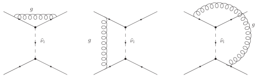
Figure 1: One-loop Feynman diagrams in the full theory.

The NLO diagrams in the full theory are shown in Fig. 1 In the full theory, all the UV divergences should be removed by the renormalization of the quark wave functions and the coupling constants. The renormalized amplitude in the full theory is

$$A_{\text{full}} =-\sum_{i}\frac{\lambda^{\prime}_{ijk}\lambda^{\prime*}_{ikj}}{m^{2}_{\tilde{\nu}}}\left\{\left[1+\frac{\alpha_{s}}{\pi}C_{F}\left(1-2\ln\frac{m_{Q}^{2}}{\mu^{2}}\right)+\frac{\alpha_{s}}{4\pi}\frac{m_{\tilde{\nu}}^{2}\ln\frac{m_{Q}^{2}}{m_{q}^{2}}+m_{Q}^{2}\ln\frac{m_{q}^{2}}{m_{\tilde{\nu}}^{2}}}{m_{\tilde{\nu}}^{2}-m_{Q}^{2}}\right]\braket{Q_{1}}_{\text{tree}}\right.$$

$$\qquad\left.-\frac{\alpha_{s}}{4\pi}\frac{1}{N}\frac{m_{\tilde{\nu}}^{2}\ln\frac{m_{Q}^{2}}{m_{q}^{2}}+m_{Q}^{2}\ln\frac{m_{q}^{2}}{m_{\tilde{\nu}}^{2}}}{m_{\tilde{\nu}}^{2}-m_{Q}^{2}}\braket{Q_{2}}_{\text{tree}}\right\},$$ (19)

where $C_{F}=4/3$, $N=3$ is the number of colors, and $\braket{Q_{i}}_{\text{tree}}$ is the tree level matrix elements of the operators.

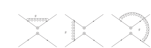
Figure 2: The next-to-leading-order corrections in the effective theory.

In the effective theory, there are remaining UV divergences after taking into account the quark field renormalization, which must be canceled by the renormalization of the effective operators. Calculating the diagrams in Fig. 2 with the insertion of the operators $Q_{1}$ and $Q_{2}$, we get the following amplitudes after quark field renormaliztion:

$$\braket{Q_{1}^{0}} =\left[1+\frac{\alpha_{s}}{2\pi}C_{F}\left(\frac{3}{\hat{\epsilon}}+2-4\ln\frac{m_{Q}^{2}}{\mu^{2}}\right)+\frac{\alpha_{s}}{4\pi}\ln\frac{m_{Q}^{2}}{m_{q}^{2}}\right]\braket{Q_{1}}_{\text{tree}}-\frac{\alpha_{s}}{4\pi}\frac{1}{N}\ln\frac{m_{Q}^{2}}{m_{q}^{2}}\braket{Q_{2}}_{\text{tree}},$$ (20)

$$\braket{Q_{2}^{0}} =\frac{\alpha_{s}}{4\pi}\left(\frac{3}{\hat{\epsilon}}+1-3\ln\frac{m_{Q}^{2}}{\mu^{2}}-\frac{1}{N}\ln\frac{m_{Q}^{2}}{m_{q}^{2}}\right)\braket{Q_{1}}_{\text{tree}}$$

$$\qquad+\left[1-\frac{\alpha_{s}}{4\pi}\frac{1}{N}\left(\frac{3}{\hat{\epsilon}}+1-3\ln\frac{m_{Q}^{2}}{\mu^{2}}\right)+\frac{\alpha_{s}}{2\pi}C_{F}\left(1-\ln\frac{m_{Q}^{2}}{\mu^{2}}\right)+\frac{\alpha_{s}}{4\pi}\ln\frac{m_{Q}^{2}}{m_{q}^{2}}\right]\braket{Q_{2}}_{\text{tree}},$$ (21)

where $1/\hat{\epsilon}=1/\epsilon-\gamma_{E}+\ln{4\pi}$. The renormalization constant matrix for the two operators is

$$\hat{Z}_{Q}=1+\frac{\alpha_{s}}{4\pi}\frac{1}{\hat{\epsilon}}\begin{pmatrix}8&0\\ 3&-1\end{pmatrix},$$ (22)

from which we obtain the anomalous dimension matrix:

$$\hat{\gamma}_{Q}=-\frac{\alpha_{s}}{2\pi}\begin{pmatrix}8&0\\ 3&-1\end{pmatrix}.$$ (23)

Our results of anomalous dimensions agree with those in Ref. general anomalous dimension .

Matching the results in the full theory and the effective theory, we extract the Wilson coefficients:

$$C_{1}(m_{\tilde{\nu}}) =-\sum_{i}\frac{\lambda^{\prime}_{ijk}\lambda^{\prime*}_{ikj}}{m^{2}_{\tilde{\nu}}}\left(1+\frac{\alpha_{s}}{4\pi}\frac{x\ln{x}}{1-x}\right),$$ (24)

$$C_{2}(m_{\tilde{\nu}}) =~{}~{}\sum_{i}\frac{\lambda^{\prime}_{ijk}\lambda^{\prime*}_{ikj}}{m^{2}_{\tilde{\nu}}}\frac{\alpha_{s}}{4\pi}\frac{1}{N}\frac{x\ln{x}}{1-x},$$ (25)

where $x=m_{Q}^{2}/m^{2}_{\tilde{\nu}}$. These coefficients satisfy the renormalization group equations

$$\frac{d}{d\ln\mu}\begin{pmatrix}C_{1}(\mu)\\ C_{2}(\mu)\end{pmatrix}=\hat{\gamma}_{Q}^{T}(\alpha_{s}(\mu))\begin{pmatrix}C_{1}(\mu)\\ C_{2}(\mu)\end{pmatrix},$$ (26)

from which we can solve the Wilson coefficients for arbitrary scale $\mu$.

$\Delta m_{B}$, $S_{J/\psi K_{s}(\phi)}$ are defined in terms of the matrix element $\bra{\bar{B}_{s(d)}}\mathcal{H}^{\Delta B=2}_{eff}\ket{B_{s(d)}}$, which can be written as

$$\bra{\bar{B}_{s(d)}}\mathcal{H}^{\Delta B=2}_{eff}\ket{B_{s(d)}}=\mathcal{A}_{SM}+\mathcal{A}_{RPV}=\mathcal{A}_{SM}(1+\frac{\mathcal{A}_{RPV}}{\mathcal{A}_{SM}}),$$ (27)

where $\mathcal{A}_{SM}$ and $\mathcal{A}_{RPV}$ denote matrix elements of the SM and the MSSM-RPV effective hamiltanian, respectively. With the above matrix element, $\Delta m_{B}$ and $S_{J/\psi K_{s}(\phi)}$ can be expressed

$$\Delta m_{B}=2\left|\bra{\bar{B}_{s(d)}}\mathcal{H}^{\Delta B=2}_{eff}\ket{B_{s(d)}}\right|=\Delta m^{SM}_{B}\left|1+\frac{\mathcal{A}_{RPV}}{\mathcal{A}_{SM}}\right|,$$

$$S_{J/\psi K_{s}(\phi)}=\text{sin}\left(2\beta_{(s)}+\text{arg}\left(1+\frac{\mathcal{A}_{RPV}}{\mathcal{A}_{SM}}\right)\right),$$ (28)

where $\Delta m^{SM}_{B}$ and $\beta_{(s)}$ denotes the SM contributions, respectively. In Eq.(28), hadronic uncertainties arising from hadron decay constants cancel between $\mathcal{A}_{SM}$ and $\mathcal{A}_{RPV}$, and hadronic uncertainties remain only in $\Delta m^{SM}_{B}$ and $\beta_{(s)}$. As for $K^{0}-\bar{K}^{0}$ mixing, $\Delta m_{K}$ can be obtained straightforwardly.

IV Numerical results

In this section we present our numerical results. The SUSY scale is taken to be the mass of the sneutrino $m_{\tilde{\nu}}$. The CKM matrix elements are parametrized in the Wolfenstein convention with four parameters $A=0.809$, $\lambda=0.2272$, $\rho=0.197$ and $\eta=0.339$. The other standard model parameters are taken to be $G_{F}=1.16637^{-5}$ GeV^-2, $\alpha_{s}(m_{Z})=0.118$, $m_{t}=173$ GeV Bparameter . The mass of B meson and K meson are $m_{B_{s}}=5367.5$ MeV, $m_{B_{0}}=5279.4$ MeV and $m_{K}=497.648$ MeV Bparameter . The time-dependent CP asymmetry in $B_{d}$ decay $S_{J/\psi K_{s}}=0.687^{+0.032}_{-0.032}$ Bparameter . The recent experimental values of the mass differences of the $B_{d}$ and $K^{0}$ mesons mixing are $\Delta{m_{K}}=(0.5292\pm 0.0009)\times 10^{-2}$ ps^-1, $\Delta{m_{B_{d}}}=0.507^{+0.005}_{-0.005}$ ps^-1 Bparameter , and $\Delta{m_{s}}$ is shown in Eq. (1).

In our numerical calculations, we first neglect the uncertainties from the hadronic parameters in the SM and assume that the predictions of the SM can reproduce the central values of the experimental data. Thus we demand that the RPV contributions must not exceed the experimental upper and lower bounds of the corresponding data.

First, we consider the new measurement of $B_{s}-\bar{B}_{s}$ mixing, which can constrain the combination $\Lambda_{32}\equiv\sum\limits_{i}\lambda^{\prime}_{i32}\lambda^{\prime*}_{i23}$ once the sneutrino mass is given. Fig. 3 shows the allowed region in the $\Lambda_{32}-m_{\tilde{\nu}}$ plane, where the gray area and the dark area is the allowed region extracted from the leading-order amplitude. We find that with the new data, the couplings are constrained to the level of $10^{-9}$. After including the NLO QCD corrections, the gray area is excluded and only the dark area survives. One can see that since the NLO QCD effects increase the resulting mass difference, the bound is more stringent (about 50% lower) than that from LO calculations. If setting $m_{\tilde{\nu}}=100$ GeV, the bounds on $\Lambda_{32}$ from the calculations of LO and NLO are

$$\Lambda_{32}<4.6\times 10^{-9}\text{(LO)},\quad 2.4\times 10^{-9}\text{(NLO)},$$ (29)

respectively.

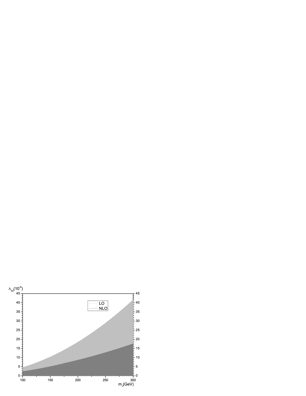
Figure 3: The bounds for $\sum\limits_{i}\lambda^{\prime}_{i32}\lambda^{\prime*}_{i23}$ vary with the mass of the sneutrino. The gray area and the dark area are the allow region extracted from the LO amplitude. After NLO corrections, the gray area is excluded and only the dark area survives.

Fig. 4 and Fig. 5 show the constraints on the combination $\Lambda_{31}\equiv\sum\limits_{i}\lambda^{\prime}_{i31}\lambda^{\prime*}_{i13}$ from $B_{0}-\bar{B}_{0}$ mixing and $\Lambda_{21}\equiv\sum\limits_{i}\lambda^{\prime}_{i21}\lambda^{\prime*}_{i12}$ from $K_{0}-\bar{K}_{0}$ mixing. The situation here is similar to that in $B_{s}-\bar{B}_{s}$ mixing: the NLO QCD corrections increase the mass differences and thus give more strong constraints on the combinations of couplings of MSSM-RPV. At the reference point $m_{\tilde{\nu}}=100$ GeV, the bounds are

$$\Lambda_{31}<2.9\times 10^{-10}\text{(LO)},\quad 1.5\times 10^{-10}\text{(NLO)},$$ (30)

$$\Lambda_{21}<8.8\times 10^{-14}\text{(LO)},\quad 2.8\times 10^{-14}\text{(NLO)}.$$ (31)

Above bounds are two and four orders of magnitude stronger than ones given in Ref. Rparity1 , as shown in Eq. (3), which is due to the fact that the updated data of the measurements and the contributions from the SM have been considered in our calculations.

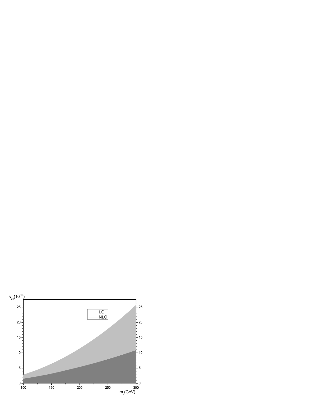
Figure 4: The bounds for $\sum\limits_{i}\lambda^{\prime}_{i31}\lambda^{\prime*}_{i13}$ vary with the mass of the sneutrino.

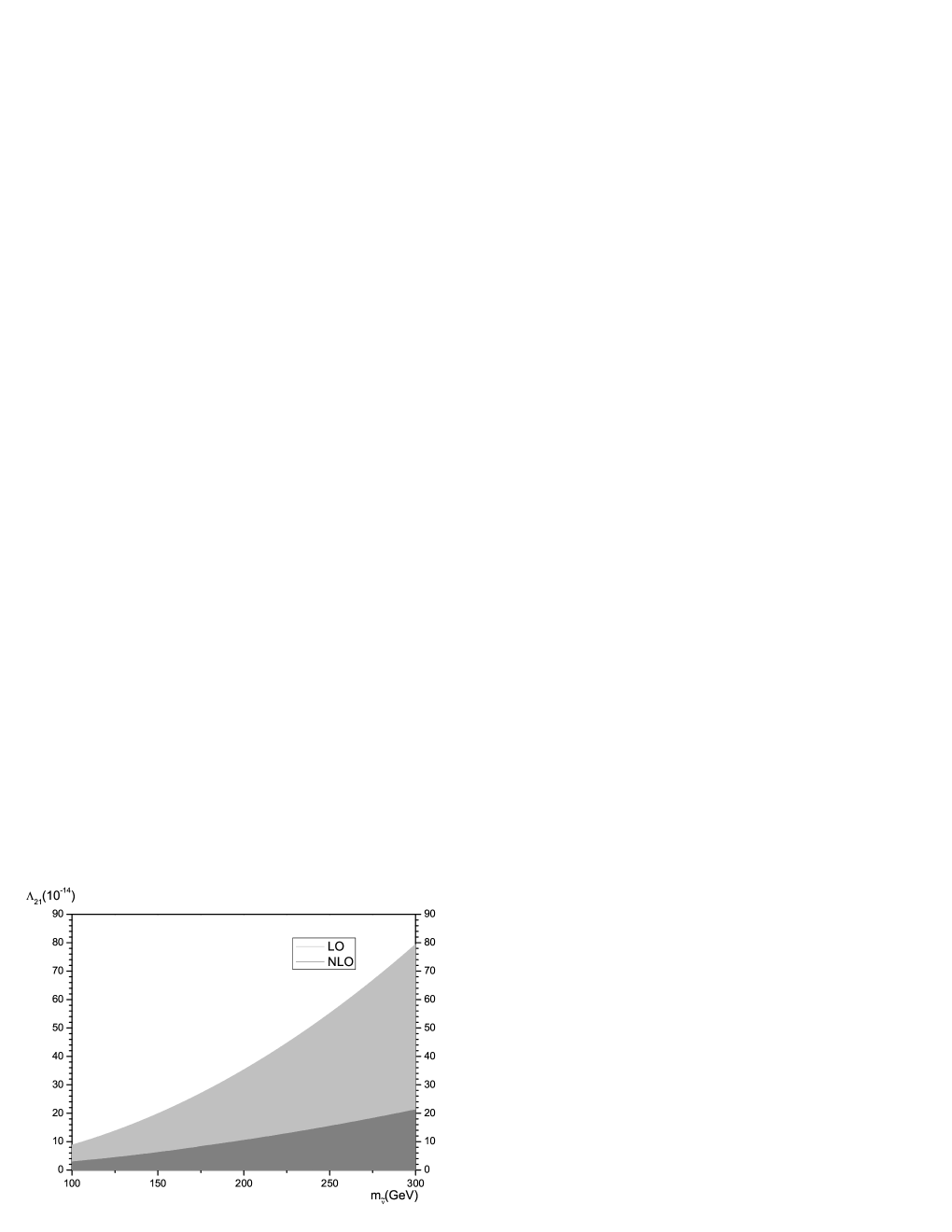
Figure 5: The bounds for $\sum\limits_{i}\lambda^{\prime}_{i21}\lambda^{\prime*}_{i12}$ vary with the mass of the sneutrino.

We further consider the situation that the hadronic uncertainties are involved. In this case, the bounds on the combinations of couplings in MSSM-RPV are looser than those in Eqs. (29), (30) and (31). The new bounds from the three observables are

$$\Lambda_{32} <12.392\times 10^{-8}\quad\text{(LO)},$$

$$<6.481\times 10^{-8}\quad\text{(NLO)};$$

$$\Lambda_{31} <7.833\times 10^{-9}\quad\text{(LO)},$$

$$<4.096\times 10^{-9}\quad\text{(NLO)};$$

$$\Lambda_{21} <3.47\times 10^{-11}\quad\text{(LO)},$$

$$<1.39\times 10^{-11}\quad\text{(NLO)},$$ (32)

respectively.

We also discuss the situation that $\Lambda_{ij}$ is complex, and parametrize the combinations of relevant couplings as $\Lambda_{ij}=|\Lambda_{ij}|e^{2i\sigma_{ij}}$, where $ij$ can be $32$ and $31$. After assuming arbitrary phases $\sigma_{ij}$, we can obtain constraints on the magnitude $|\Lambda_{ij}|$. Fig. 6 and Fig. 7 shows the the allowed range of $\Lambda_{32}$ and $\Lambda_{31}$ for $m_{\tilde{\nu}}=100$GeV, taking into account the constraints from $\Delta m_{s}$ and $\Delta m_{d}$. For the $B_{s}-\bar{B}_{s}$ mixing, $\Lambda_{32}$ is about $\mathcal{O}(10^{-9})$, while for the $B_{d}-\bar{B}_{d}$ mixing, $\Lambda_{31}$ is about $\mathcal{O}(10^{-11})$. In both figures, there are additional areas with large $|\Lambda_{ij}|$ besides ordinary areas with small $|\Lambda_{ij}|$, which correspond to ones where contributions from the MSSM-RPV are larger than those from the SM, roughly twice the SM contributions but with different signs. We do not discuss complex couplings in K system due to the fact that Eq. (13) holds only under the condition that imaginary part of $\bra{\bar{K}^{0}}\mathcal{H}_{\text{eff}}\ket{K^{0}}$ is far less than the real part.

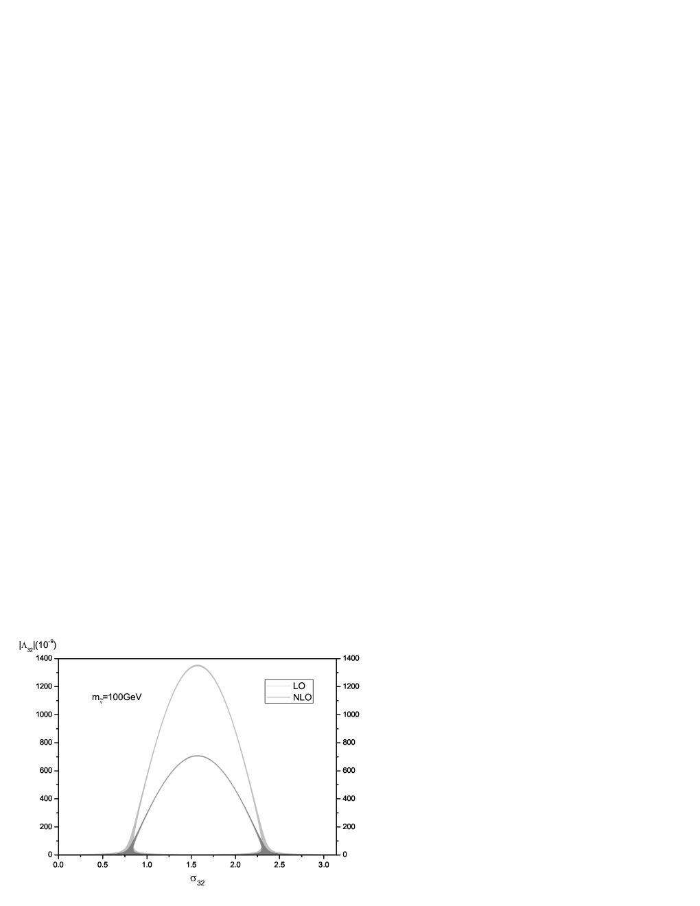
Figure 6: The allowed range of the magnitude and phase of $\sum\limits_{i}\lambda^{\prime}_{i32}\lambda^{\prime*}_{i23}$ constrained by the updated experimental data of $\Delta m_{s}$. The gray area accounts for the tree level results. When the QCD corrections are added, the allowed area is reduced to the dark area.

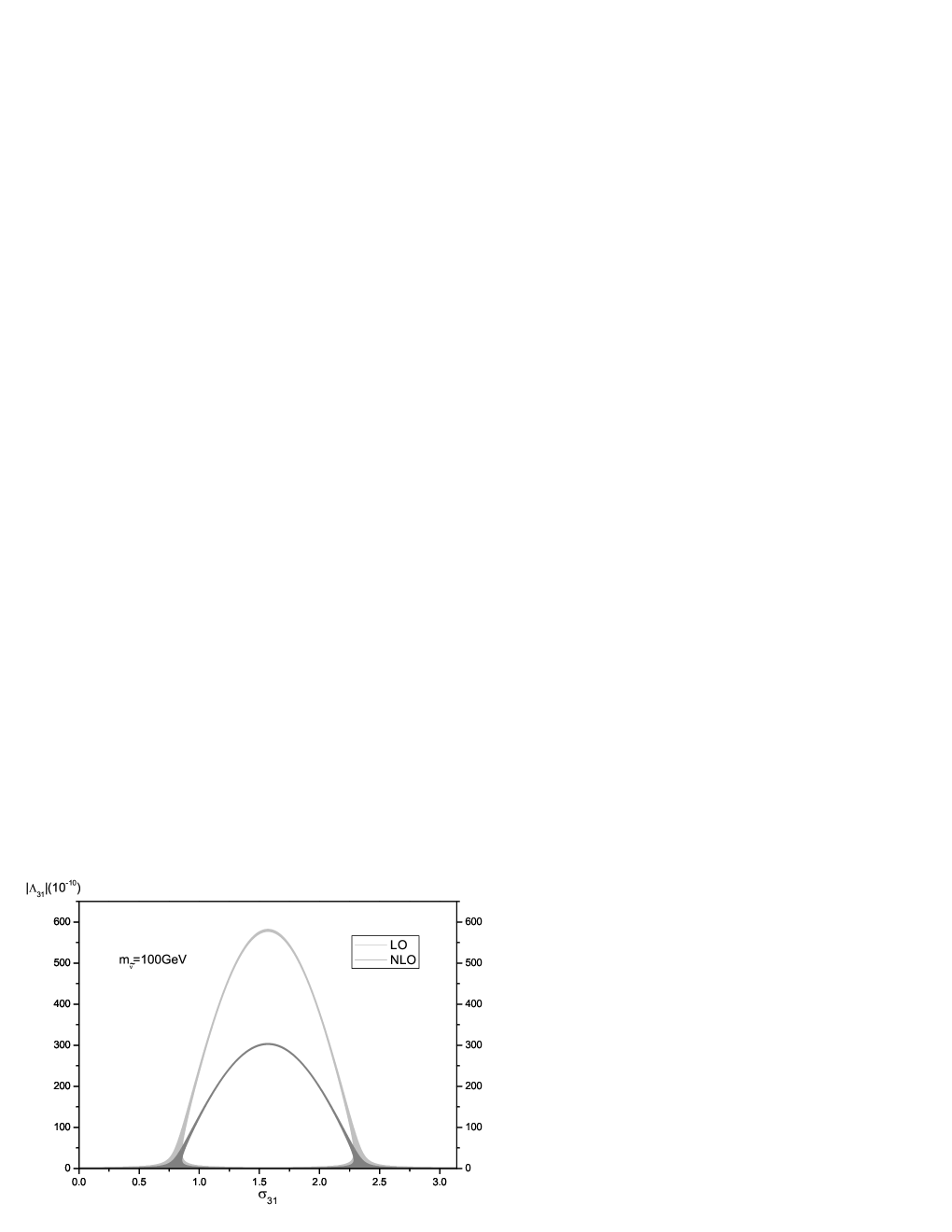
Figure 7: The allowed range of the magnitude and phase of $\sum\limits_{i}\lambda^{\prime}_{i31}\lambda^{\prime*}_{i13}$ constrained by the experimental data of $\Delta m_{d}$.

The combinations of complex couplings can introduce new CP-violation origins, so we further investigate how the CP asymmetries in B decays constrain these combinations of couplings. Using the experimental data of $S_{J/\psi K_{s}}$ Bparameter , we plot the allowed areas of the magnitude $|\Lambda_{31}|$ and the phase $\sigma_{31}$ in Fig.8, which shows that the upper bound for $|\Lambda_{31}|$ is generally about $\mathcal{O}(10^{-10})$, except for some special values of $\sigma_{31}$. Those special values correspond to $\arg(1+\mathcal{A}_{RPV}/\mathcal{A}_{SM})=0$, and we have $\sin(2\beta_{\text{eff}})=\sin(2\beta)$. In fact, another area with $\arg(1+\mathcal{A}_{RPV}/\mathcal{A}_{SM})=\pi-4\beta$ also survives from constraint of experiment data of $S_{J/\psi K_{s}}$, however, this possibility has been excluded by an angular analysis of $B^{0}\rightarrow J/\psi K^{*0}$ and a time-dependent Dalitz plot analysis of $B^{0}\rightarrow\bar{D}^{0}h^{0}(h^{0}=\pi^{0},\eta^{0},\omega)$piminus2beta . For the CP asymmetry in $B_{s}$ decays, although there is no experimental data of $S_{J/\psi\phi}$ currently, future LHCb experiment will provide enough data to reach $\sigma_{stat}(S_{J/\psi\phi})\approx 0.03$ in the first year LHCb , which would provide a strong constraint on new physics. So we assume $S_{J/\psi\phi}=0.04\pm 0.03$ and plot constraints on $|\Lambda_{32}|$ and $\sigma_{32}$ in Fig.9, which shows that the upper bound for $|\Lambda_{32}|$ is about $\mathcal{O}(10^{-8})$ except for some special values of $\sigma_{32}$ similar to the case of $S_{J/\psi K_{s}}$.

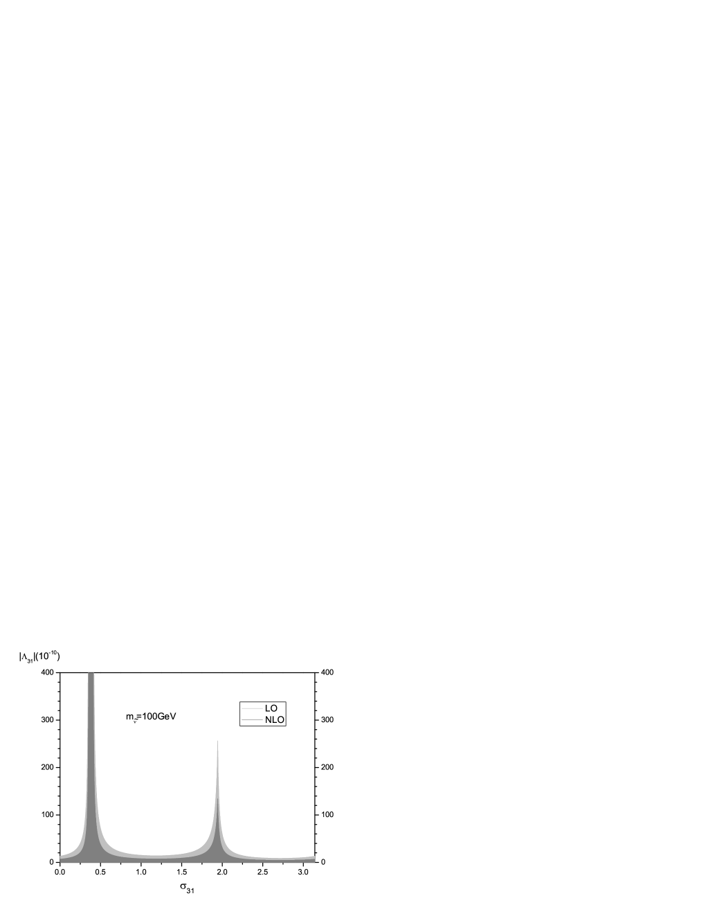
Figure 8: The allowed range of the magnitude and phase of $\sum\limits_{i}\lambda^{\prime}_{i31}\lambda^{\prime*}_{i13}$ using experimental data of $S_{J/\psi K_{s}}$.

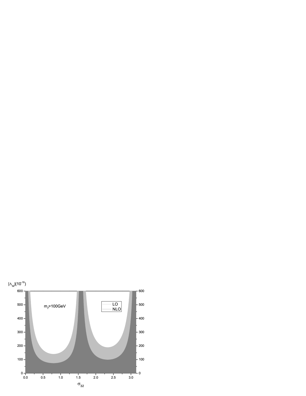
Figure 9: The allowed range of the magnitude and phase of $\sum\limits_{i}\lambda^{\prime}_{i32}\lambda^{\prime*}_{i23}$, assuming the first year LHCb data provide an experiment measurement $S_{J/\psi\phi}=0.04\pm 0.03$.

In conclusion, using the updated data, we have calculated contributions to $B_{s}-\bar{B}_{s}$ mixing, $B_{d}-\bar{B}_{d}$ mixing and $K^{0}-\bar{K}^{0}$ mixing in the framework of the minimal supersymmetric standard model with R-parity violation including NLO QCD corrections, and presented new constraints on the relevant couplings of MSSM-RPV. Our results show that upper bound on the relevant combination of couplings of $B_{s}-\bar{B}_{s}$ mixing is of the order $10^{-9}$, and upper bounds on the relevant combinations of couplings of $B_{d}-\bar{B}_{d}$ mixing and $K^{0}-\bar{K}^{0}$ mixing are two and four orders of magnitude stronger than ones reported in Ref. Rparity1 , respectively. We also discussed the case of complex couplings and showed that how the relevant combinations of couplings are constrained by the updated experiment data of $B_{s}-\bar{B}_{s}$, $B_{d}-\bar{B}_{d}$ mixing and time-dependent CP asymmetry $S_{J/\psi K_{s}}$, and future possible observations of $S_{J/\psi\phi}$ at LHCb, respectively.

$Note~{}added$. While preparing this manuscript the paper of RPVnew appeared where the same coupling combination from $B_{s}-\bar{B}_{s}$ mixing is also discussed. However, the authors of RPVnew mainly dealt with contributions through the box diagram. Our results induced by the tree-level diagram is a few orders of magnitude stronger than theirs.

References

(1) V. Abazov et al. (D0 Collaboration), Phys. Rev. Lett. 97, 021802 (2006).
(2) A. Abulencia et al. (CDF collaboration), Phys. Rev. Lett. 97, 062003
(2006); hep-ex/0609040.
(3) Monika Blanke, Andrzej J. Buras, Diego Guadagnoli, Cecilia
Tarantino, hep-ph/0604057.
(4)
Z. Ligeti, M. Papucci and G. Perez, Phys. Rev. Lett. 97 101801 (2006).
(5)
P. Ball and R. Fleischer, hep-ph/0604249.
(6) Alakabha Datta, Phys. Rev. D74 (2006) 014022.
(7) UTfit Collaboration: M. Bona, et al, Phys. Rev. Lett. 97, 151803
(2006).
(8) M. Ciuchini, L. Silvestrini, Phys. Rev. Lett. 97 (2006) 021803.
(9) M. Blanke, A. J. Buras, A. Poschenrieder, C. Tarantino, S. Uhlig, A.
Weiler, hep-ph/0605214.
(10) Seungwon Baek, Jong Hun Jeon, C. S. Kim, hep-ph/0607113.
(11) Kingman Cheung, Cheng-Wei Chiang, N. G. Deshpande, J.
Jiang, hep-ph/0604223.
(13) Gino Isidori, Paride Paradisi, Phys. Lett. B639 (2006)
499-507.
(14) J. K. Parry, hep-ph/0606150; hep-ph/0608192.
(15) G. Farrar, P. Fayet, Phys. Lett. B 76 (1978) 575; R. Barbier, et al, Phys. Rept. 420 (2005)
1-202.
(16) D. Choudhury, P. Roy, Phys. Lett.B 378 (1996) 153-158.
(17) [Heavy Flavor Averaging Group (HFAG)], hep-ex/0603003.
(18) Andrzej J. Buras, hep-ph/9806471.
(19) F. J. Gilman, M. B. Wise, Phys. Rev. D 27 1128(1983).
(20) A. J. Buras, M. Jamin, P. H. Weisz, Nucl. Phys. B347, 491 (1990); J.
Urban, F. Krauss, U. Jentschura and G. Soff, Nucl. Phys. B523,
40(1998).
(21) T. Inami and C. S. Lim, Prog. Theor. Phys. 65, 297 (1981); 65, 1772(E)
(1981).
(22) S. Herrlich and U. Nierste, Nucl. Phys. B419, 292(1994); Phys. Rev. D52,
6505(1995) ; Nucl. Phys. B476, 27(1996).
(23) G. C. Branco, L. Lavoura, J. P. Silva, CP Violation, Claredon
Press Oxford, 1999.
(24) C. R. Allton, L. Conti, A. Donini, V. Gimenez, L. Giusti, G.
Martinelli, M. Talevi, A. Vladikas, Phys. Lett. B453 (1999) 30-39.
(25) D. Becirevic et al., Nucl. Phys. B634, 105 (2002); D. Becirevic, V.
Gimenez, G. Martinelli, M. Papinutto, and J. Reyes, JHEP. 04, 025
(2002); Nucl. Phys. B (Proc. Suppl.) 106. 385 (2002).
(26)
M. Ciuchini, E. Franco, V. Lubicz, G. Martinelli, I. Schimemi, L.
Silvestrini, Nucl. Phys. B523 (1998) 501-525.
(27) W.-M. Yao, et al, (Paticle Data Group), Review of Particle Physics,
J. Phys. G: Nucl. Part. Phys. 33 (2006) 1.
(28) B. Aubert et al., [BABAR
colaboration], Phys. Rev. D71, 032005 (2005); R. Itoh
et al., [Belle colaboration], Phys. Rev. Lett. 95, 091601
(2005); K Abe et al., [Belle colaboration], hep-ex/0507065;
For a comprehensive review, see Robert Fleischer, hep-ph/0608010.
(29) O. Schneider, talk given at the Workshop on “Flavour in the era of
LHC” First meeting, CERN, 2005,
http://lhcb-doc.web.cern.ch/lhcb-doc/presentations/conferencetalks/
postscript/2005presentations/Schneider_epfl.pdf.