Dimension-2 condensates, $\zeta$-regularization and large-$N_{c}$ Regge Models

Abstract

Dimension-2 and -4 gluon condensates are re-analyzed in large-$N_{c}$ Regge models with the $\zeta$-function regularization which preserves the spectrum in any $\bar{q}q$ channel separately. We demonstrate that the signs and magnitudes of both condensates can be properly described within the framework.

The dimension-2 gluon condensate, corresponding to vacuum expectation values of a gauge-invariant non-perturbative and non-local operator and generating the lowest $1/Q^{2}$ power corrections, was proposed long ago Celenza:1986th and has been determined in instanton-model studies Hutter:1993sc , phenomenological QCD sum-rule re-analyses Dominguez:1994qt ; Chetyrkin:1998yr , theoretical considerations Gubarev:2000eu ; Gubarev:2000nz ; Kondo:2001nq ; Verschelde:2001ia ; Narison:2001ix , non-local quark models Dorokhov:2003kf , and lattice simulations at zero Boucaud:2001st ; RuizArriola:2004en and finite Megias:2005ve temperatures. In the present contribution we re-examine our recent findings RuizArriola:2006gq , namely, that within the large-$N_{c}$ expansion these $1/Q^{2}$ corrections appear naturally within the Regge framework, on the light of $\zeta$-regularization. We show that the signs and magnitudes of both the dimension-2 and -4 condensates can be accommodated comfortably with reasonable values of the parameters of the hadronic spectra. Many works compare Regge models to the Operator Product Expansion (OPE) Golterman:2001nk ; Beane:2001uj ; Simonov:2001di ; Afonin:2003gp ; Afonin:2004yb but besides Afonin:2004yb the dimension-2 condensate has been ignored.

We begin with a simple quantum-mechanical derivation of the (radial) Regge spectrum. For two relativistic scalar quarks of mass $m$ interacting via a linear confining potential the mass operator in the CM frame is given by

$$M=2\sqrt{\vec{p}^{2}+m^{2}}+\sigma_{S}r,$$ (1)

where $\sigma_{S}$ is the (scalar) string tension and $\vec{p}$ and $r$ are the relative momentum and distance respectively. Squaring the $\sqrt{\vec{p}^{2}+m^{2}}$ yields an equivalent Schrödinger operator. Let us assume $L=0$ and $m=0$ for simplicity, such that $\vec{p}^{2}=p_{r}^{2}+L^{2}/r^{2}$. For excited radial states the Bohr-Sommerfeld semiclassical quantization condition holds,

$$2\int_{0}^{a}p_{r}dr=2\pi(n+\alpha),$$ (2)

where the turning point is given by $a=M/\sigma_{S}$ and $\alpha$ is of order of unity. The integral is trivial and leads to

$$M^{2}_{n}=4\pi\sigma_{S}(n+\alpha)=2\pi\sigma(n+\alpha),$$ (3)

a (radial) Regge mass spectrum which in terms of the spinor string tension $\sigma=2\sigma_{S}$ (the factor depends on the type of interaction Goebel:1989sd ) is well fulfilled experimentally for mesons Anisovich:2000kx and signals confinement for the quark states. For large meson masses, the level density becomes

$$\rho(M^{2}) = \sum_{n}\delta(M^{2}-M_{n}^{2})\to\int dn\delta(M^{2}-M_{n}^{2})$$ (4)

$$= \frac{dn}{dM^{2}}=\frac{1}{\pi}\int_{0}^{a}\frac{dr}{p_{r}}=\frac{1}{2\pi\sigma}$$

which is a constant. Inclusion of finite quark mass corrections is straightforward, yielding

$$\frac{dn}{dM^{2}}=\frac{1}{2\pi\sigma}\sqrt{1-\frac{4m^{2}}{M^{2}}}\quad{\rm for}\quad M^{2}\geq 4m^{2}\,.$$ (5)

Note that this corresponds to the two-body phase space factor appearing in the absorptive part of two-point correlators. Thus at large energies the WKB approximation holds and $\rho(M^{2})$ looks like the phase space of two free particles, featuring the quark-hadron duality.

The best way to look the $q\bar{q}$ level density is to consider two point correlation functions in different channels,

$$i\Pi^{\mu a,\nu b}(q) = \int d^{4}xe^{-iq\cdot x}\langle 0|T\left\{J^{\mu a}(x)J^{\nu b}(0)\right\}|0\rangle$$ (6)

$$= \Pi(q^{2})\,\left(q^{\mu}q^{\nu}-g^{\mu\nu}q^{2}\right)\delta^{ab},$$

where current conservation for both the vector and axial currents has explicitly been used. At high Euclidean momentum OPE can be performed. Equivalently, in the Euclidean coordinate space one has

$$\langle J_{\mu}(x)J_{\nu}(0)\rangle = \left(g^{\mu\nu}\partial^{2}-\partial^{\mu}\partial^{\nu}\right)\Pi(x).$$ (7)

The function $\Pi(x)$ has dimension $x^{-4}$. Thus, at short distances one expects to have (up to possible logarithms)

$$\Pi(x) = \frac{O_{0}}{x^{4}}+\frac{O_{2}}{x^{2}}+\frac{O_{4}}{x^{0}}+\frac{O_{6}}{x^{2}}+\dots$$ (8)

We digress that the term containing $O_{2}$ is very special, since it yields a contribution of the form

$$\left(g^{\mu\nu}\partial^{2}-\partial^{\mu}\partial^{\nu}\right)\frac{1}{x^{2}} = \frac{g^{\mu\nu}x^{2}-4x^{\mu}x^{\nu}}{x^{4}},$$ (9)

which in addition of being conserved is also traceless. Thus, contracting and taking the derivative $\partial^{\alpha}$ do no commute. There is no traceless and transverse term in momentum space, since conservation implies the form $A(q^{\mu}q^{\nu}-q^{2}g^{\mu\nu})$ but tracelessness requires $A=0$. This problem appears in chiral quark models; the dimension-2 object is the constituent quark mass squared, $O_{2}\sim\langle\sigma^{2}+\vec{\pi}^{2}\rangle\sim M^{2}$.

Recent discussions incorporate $O_{2}$ in OPE. From Narison:2001ix we get up to dimension 6 in the chiral limit

$$\Pi_{V+A}(Q^{2}) = \frac{1}{4\pi^{2}}\Big{\{}-\left(1+\frac{\alpha_{S}}{\pi}\right)\log\frac{Q^{2}}{\mu^{2}}$$

$$- \frac{\alpha_{S}}{\pi}\frac{\lambda^{2}}{Q^{2}}+\frac{\pi}{3}\frac{\langle\alpha_{S}G^{2}\rangle}{Q^{4}}+\frac{256\pi^{3}}{81}\frac{\alpha_{S}\langle\bar{q}q\rangle^{2}}{Q^{6}}\Big{\}},$$

$$\Pi_{V-A}(Q^{2}) = -\frac{32\pi}{9}\frac{\alpha_{S}\langle\bar{q}q\rangle^{2}}{Q^{6}},$$ (10)

where $\lambda^{2}$ corresponds to the dimension-2 condensate.

In the large-$N_{c}$ limit one has (up to subtractions) Pich:2002xy

$$\Pi_{V}(Q^{2})=\sum_{V}\frac{F_{V}^{2}}{M_{V}^{2}+Q^{2}}+c.t.,$$ (11)

where the sum involves infinitely many resonances. This function satisfies a dispersion relation of the form

$$\Pi_{V}(Q^{2})=\int_{0}^{\infty}ds\frac{Q^{2}}{s}\frac{\rho_{V}(s)}{s+Q^{2}},$$ (12)

with one subtraction, with the spectral function

$$\rho_{V}(s)=\frac{1}{\pi}{\rm Im}\Pi_{V}(s)=\sum_{V}F_{V}^{2}\delta(s-M_{V}^{2}).$$ (13)

At large values of the squared CM energy $s$ it becomes

$$\!\!\!\!\!\!\!\rho_{V}(s) \to \int_{0}^{\infty}\!\!\!\!F_{V}^{2}\delta(s-M_{V}^{2})dn=F_{V}(n)^{2}\frac{dn}{dM_{V}^{2}}\Big{|}_{M_{V}^{2}=s}\!\!.$$ (14)

Matching to the free massless quark result
$\rho_{V}(s)=N_{c}/(12\pi^{2})\theta(s)$ gives at large values of $n$

$$F_{V}(n)^{2}\frac{dn}{dM_{V}^{2}}\to\frac{N_{c}}{3}\frac{1}{4\pi^{2}}.$$ (15)

For constant $F_{V}$ this implies the asymptotic spectrum $M_{V}^{2}\to 2\pi\sigma n$ with the string tension given by $2\pi\sigma=24\pi^{2}F_{V}^{2}/N_{c}$. If we identify $F_{V}=154{\rm MeV}$ from the $\rho\to 2\pi$ decay Ecker:1988te which corresponds to only one resonance we get $\sqrt{\sigma}=546{\rm MeV}$. Lattice calculations Kaczmarek:2005ui provide $\sqrt{\sigma}=420{\rm MeV}$. Including infinitely many resonances improves the value of $\sigma$.

In dimensional regularization the coupling of the resonance to the current acquires an additional dimension $F_{V}\to F_{V}\mu^{\epsilon}$ with $\epsilon=d-4$. By choosing $\mu=M_{V}$ one gets $F_{V}^{2}\to F_{V}^{2}M_{V}^{2\epsilon}$. The regularized correlator is an analytic function for $Q^{2}<m_{\rho}^{2}$ (the lowest mass), so we can Taylor-expand at small $Q^{2}$. We can then regularize the finite coefficients of the expansion and proceed by analytic continuation both in $Q^{2}$ and $\epsilon$. The regularization only acts for truly infinitely many resonances. At large Euclidean momenta one gets

$$\Pi_{V}(Q^{2})=\sum_{V}F_{V}^{2}M_{V}^{2\epsilon}-\sum_{V}F_{V}^{2}\frac{M_{V}^{2+2\epsilon}}{Q^{2}}+\dots$$ (16)

The coefficients of powers in $1/Q^{2}$ of the expansion are convergent provided one computes the sum first and then takes the limit $\epsilon\to 0$ corresponding to the use of the $\zeta$ function regularization (see e.g. Salcedo:1994qy ),

$$\sum_{V}F_{V}^{2}M_{V}^{2n}\equiv\lim_{s\to n}\sum_{V}F_{V}^{2}M_{V}^{2s}\,.$$ (17)

In other words, one may expand formally at large $Q^{2}$ and re-interpret the result by means of the $\zeta$-function regularization. Using the axial-axial correlator at large $N_{c}$,

$$\Pi_{A}(Q^{2})=\frac{f^{2}}{Q^{2}}+\sum_{A}\frac{F_{A}^{2}}{M_{A}^{2}+Q^{2}}+c.t.,$$ (18)

and matching to (10) yields the two Weinberg sum rules:

$$f^{2} = \sum_{A}F_{A}^{2}-\sum_{V}F_{V}^{2},\hskip 76.82243pt{\rm(WSR~{}I)}$$

$$0 = \sum_{A}F_{A}^{2}M_{A}^{2}-\sum_{V}F_{V}^{2}M_{V}^{2}.\hskip 42.67912pt{\rm(WSR~{}II)}$$

These sums are assumed to be $\zeta$-regularizated, see Eq. (17).

The simplest Regge model is given by

$$M^{2}_{V,n}=M_{V}^{2}+2\pi\sigma n,\;M^{2}_{A,n}=M_{A}^{2}+2\pi\sigma n,$$ (19)

$n=0,1,2\dots$, which is well fulfilled Anisovich:2000kx experimentally. The corresponding couplings are constant, $F_{V}=F_{A}=F$ and the $\zeta$-function regularized sums follow from

$$\sum_{n=0}^{\infty}(na+M^{2})^{s}=a^{s}\zeta\left(-s,\frac{M^{2}}{a}\right).$$ (20)

This function is analytic in the complex plane ${\rm Re}(s)\leq-1$ with the exception of $s=-1$, admitting analytic continuation to any $s$. Actually, for positive powers one gets the Bernoulli polynomials $\zeta(-k,z)=-B_{k+1}(z)/(k+1)$, where $B_{0}=1$, $B_{1}=x-1/2$, $B_{2}=x^{2}-x+1/6$, etc. An important feature of the $\zeta$-function is that it regulates each spectrum separately, i.e. under regularization one cannot apply the distributive property. For instance,

$$\sum_{n=0}^{\infty}(an+M_{V}^{2})^{0}-\sum_{n=0}^{\infty}(an+M_{A}^{2})^{0}\neq 0.$$ (21)

In other words, the difference of the regularized sums does not coincide with the regularized difference. The finite terms in the difference have to do with preserving the spectra in the vector and axial channels separately, and hence a chiral asymmetry is generated. All these $\zeta$-function results reproduce the direct asymptotic expansion of exact sums in terms of the digamma functions, but allow to discuss cases where the sums cannot be carried out before expanding in large $Q^{2}$.

The strict linear Regge model does not generate condensates with the proper signs. In RuizArriola:2006gq (see also Afonin:2006da ) we consider the following simple modification

$$M_{V,0} = m_{\rho},\;M_{V,n}^{2}=M_{V}^{2}+2\pi\sigma n,\;\;n\geq 1,$$

$$M_{A,n}^{2} = M_{A}^{2}+2\pi\sigma n,\;\;n\geq 0.$$ (22)

In words, the lowest $\rho$ mass is shifted, otherwise all is kept “universal”, including constant residues for all states. With (22) the Weinberg sum rules are (we set $N_{c}=3$)

$$M_{A}^{2} = M_{V}^{2}+8\pi^{2}f^{2},$$

$$2\pi\sigma = 8\pi^{2}F^{2}=\frac{8\pi^{2}f^{2}\left(4\pi^{2}f^{2}+{M_{V}}^{2}\right)}{4\pi^{2}f^{2}-{m_{\rho}}^{2}+{M_{V}}^{2}}.$$ (23)

When $m_{\rho}=0.77{\rm GeV}$ is fixed, the model has only one free parameter left. We may take it to be $M_{V}$, however, it is more convenient to express it through the string tension $\sigma$, which is then treated as a free parameter. Thus

$$M_{V}^{2}=\frac{-16\pi^{3}f^{4}+4\pi^{2}\sigma f^{2}-{m_{\rho}}^{2}\sigma}{4f^{2}\pi-\sigma},$$ (24)

and the condensates, obtained by matching to (10), are

$$-\frac{\alpha_{S}\lambda^{2}}{4\pi^{3}} = \frac{16\pi^{3}f^{4}-\pi\sigma^{2}+{m_{\rho}}^{2}\sigma}{16f^{2}\pi^{3}-4\pi^{2}\sigma}$$

$$\frac{\alpha_{S}\langle G^{2}\rangle}{12\pi} = 2\pi^{2}f^{4}-\pi\sigma f^{2}$$ (25)

$$+ \frac{3\sigma m_{\rho}^{2}}{8\pi^{2}}\left(\frac{{m_{\rho}}^{2}\sigma}{\left(\sigma-4f^{2}\pi\right)^{2}}-2\pi\right)+\frac{\sigma^{2}}{12}.$$

This allows to reproduce the correct signs and numbers in the range $0.48\leq\sqrt{\sigma}\leq 0.5~{}{\rm GeV}$ RuizArriola:2006gq (see Fig. 1).

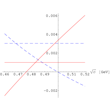
Figure 1: Dimension-2 (solid line, in GeV²) and -4 (dashed line, in GeV⁴) condensates plotted as functions of $\sqrt{\sigma}$. The horizontal lines indicate estimates from the literature.

References

• (1) L. S. Celenza and C. M. Shakin, Phys. Rev. D 34, 1591 (1986).
• (2) M. Hutter, arXiv:hep-ph/9501335.
• (3) C. A. Dominguez, Phys. Lett. B 345, 291 (1995)
• (4) K. G. Chetyrkin, S. Narison and V. I. Zakharov, Nucl. Phys. B 550, 353 (1999)
• (5) F. V. Gubarev, L. Stodolsky and V. I. Zakharov, Phys. Rev. Lett.  86, 2220 (2001)
• (6) F. V. Gubarev and V. I. Zakharov, Phys. Lett. B 501, 28 (2001)
• (7) K. I. Kondo, Phys. Lett. B 514, 335 (2001)
• (8) H. Verschelde, K. Knecht, K. Van Acoleyen and M. Vanderkelen, Phys. Lett. B 516, 307 (2001)
• (9) S. Narison and V. I. Zakharov, Phys. Lett. B 522, 266 (2001)
• (10) A. E. Dorokhov and W. Broniowski, Eur. Phys. J. C32 (2003) 79
• (11) P. Boucaud, A. Le Yaouanc, J. P. Leroy, J. Micheli, O. Pene and J. Rodriguez-Quintero, Phys. Rev. D 63, 114003 (2001)
• (12) E. Ruiz Arriola, P. O. Bowman and W. Broniowski, Phys. Rev. D 70, 097505 (2004)
• (13) E. Megias, E. Ruiz Arriola and L. L. Salcedo, JHEP 0601, 073 (2006)
• (14) E. Ruiz Arriola and W. Broniowski, Phys. Rev. D 73 (2006) 097502
• (15) M. Golterman and S. Peris, JHEP 0101, 028 (2001) ; Phys. Rev. D 67, 096001 (2003).
• (16) S. R. Beane, Phys. Rev. D 64, 116010 (2001)
• (17) Y. A. Simonov, Phys. Atom. Nucl.  65, 135 (2002) [Yad. Fiz.  65, 140 (2002)]
• (18) S. S. Afonin, Phys. Lett. B 576, 122 (2003)
• (19) S. S. Afonin, A. A. Andrianov, V. A. Andrianov and D. Espriu, JHEP 0404, 039 (2004)
• (20) C. Goebel, et al. Phys. Rev. D 41 (1990) 2917.
• (21) A. V. Anisovich, V. V. Anisovich and A. V. Sarantsev, Phys. Rev. D 62, 051502 (2000)
• (22) A. Pich, arXiv:hep-ph/0205030.
• (23) G. Ecker, J. Gasser, A. Pich and E. de Rafael, Nucl. Phys. B 321, 311 (1989).
• (24) O. Kaczmarek and F. Zantow, Phys. Rev. D 71, 114510 (2005)
• (25) S. S. Afonin and D. Espriu, arXiv:hep-ph/0602219.
• (26) L. L. Salcedo and E. Ruiz Arriola, Annals Phys.  250, 1 (1996)