Indirect detection of light neutralino dark matter in the NMSSM

Abstract

We explore the prospects for indirect detection of neutralino dark matter in supersymmetric models with an extended Higgs sector (NMSSM). We compute, for the first time, one-loop amplitudes for NMSSM neutralino pair annihilation into two photons and two gluons, and point out that extra diagrams (with respect to the MSSM), featuring a potentially light CP-odd Higgs boson exchange, can strongly enhance these radiative modes. Expected signals in neutrino telescopes due to the annihilation of relic neutralinos in the Sun and in the Earth are evaluated, as well as the prospects of detection of a neutralino annihilation signal in space-based gamma-ray, antiproton and positron search experiments, and at low-energy antideuteron searches. We find that in the low mass regime the signals from capture in the Earth are enhanced compared to the MSSM, and that NMSSM neutralinos have a remote possibility of affecting solar dynamics. Also, antimatter experiments are an excellent probe of galactic NMSSM dark matter. We also find enhanced two photon decay modes that make the possibility of the detection of a monochromatic gamma-ray line within the NMSSM more promising than in the MSSM.

I Introduction

Numerous theoretical and phenomenological motivations exist for a Minimal Supersymmetric extension of the Standard Model (MSSM). At the same time one of the attractive by-products of low energy supersymmetry is the natural occurrence in the particle content of the theory of a stable weakly interacting massive particle, the lightest neutralino, which could be the microscopic constituent of the as yet unobserved galactic halo dark matter. Another strong motivation comes from the SM hierarchy problem, originating from the large fine-tuning required by the stability of the electroweak scale to radiative corrections, originating from the large number of orders of magnitude occurring between the GUT, or the Planck, scale, and the electroweak scale itself.

Although very appealing, the MSSM has been challenged by various pieces of experimental information, and by some arguments of more theoretical nature. Among these, the LEP-II limit on the mass of the lightest CP-even Higgs Bastero-Gil:2000bw , the constraints on the masses of supersymmetric (Susy) charged or colored particles from direct searches at LEP and at the Tevatron pdg , and the so-called $\mu$ problem, i.e. the fundamental reason why the Susy Higgsino mass term $\mu$ appearing in the MSSM superpotential lies at some scale near the electroweak scale rather than at some much higher scale.

The addition of a new gauge singlet chiral multiplet, $\hat{S}$, to the particle content of the MSSM can provide an elegant solution to the mentioned $\mu$ problem of the MSSM Kim:1983dt . The so-called Next to Minimal Supersymmetric Standard Model (NMSSM) Ellis:1988er is an example of one such minimal extension that also alleviates the little fine tuning problem of the MSSM, arising from the non-detection of a neutral CP-even Higgs at LEP-II Bastero-Gil:2000bw .

A further motivation to go beyond the MSSM comes from Electro-Weak Baryogenesis (EWB), i.e. the possibility that the baryon asymmetry of the Universe originated through electro-weak physics at the electro-weak phase-transition in the Early Universe. Although still a viable scenario within the MSSM ewb , EWB generically requires the Higgs mass to be in the narrow mass range above the current LEP-II limits and below $\simeq 120$ GeV, a rather unnatural mass splitting between the right-handed and the left-handed stops (the first one required to lie below the top quark mass, and the other in the multi-TeV range), CP violation at levels sometimes at odds with electric dipole moment experimental results, and, generically, a very heavy sfermion sector ewbmssm . In contrast, the NMSSM provides extra triscalar Higgs couplings which hugely facilitate the occurrence of a more strongly first-order EW phase transition, and extra CP violating sources, relaxing most of the above mentioned requirements in the context of the MSSM ewbnmssm ; Funakubo:2005pu .

One of the chief remaining cosmological issues associated with the NMSSM, the cosmological domain wall problem Abel:1995wk , caused by the discrete $\mathbb{Z}_{3}$ symmetry of the NMSSM, can be circumvented by introducing non-renormalizable Planck-suppressed operators Panagiotakopoulos:1998yw .

The Higgs sector of the NMSSM contains three CP-even and two CP-odd scalars, which are mixtures of MSSM-like Higgses and singlets. Also, the neutralino sector contains five mass-eigenstates, instead of the four in the MSSM, each of which has, in addition to the four MSSM components, a singlino component, the latter being the fermionic partner of the extra singlet scalars. The extended Higgs and neutralino sectors weaken the mass bounds for both the Higgs bosons and the neutralinos. Very light neutralinos and Higgs bosons, even in the few GeV range, are in fact not excluded in the NMSSM Franke:1994hj (see also Ellis:1988er ; Franke:1995tc ; the particle spectrum with the dominant 1-loop and 2-loop corrections to the Higgs sector is available via the numerical code Nmhdecay Ellwanger:2005dv ).

The cosmology of Dark Matter singlinos has been addressed long ago in Ref. Greene:1986th , while the LSP relic abundance in the NMSSM was first calculated in Abel:1992ts . Constraints from electroweak symmetry breaking and GUT scale universality were added in Stephan:1997ds . More recently, the computer code micrOMEGAs Belanger:2006is , has been extended to allow for the relic density calculation in the NMSSM Belanger:2005kh .

The implications for the direct detection of NMSSM neutralinos were first studied in Bednyakov:1998is , where light neutralinos ($\sim$ 3 GeV) with acceptable relic abundance and sufficiently large expected event rates for direct detection with a ⁷³Ge-detector were found in different domains of the parameter space, when the gaugino unification relation Stephan:1997ds was relaxed. In Cerdeno:2004xw , the theoretical predictions for the spin-independent neutralino-proton cross section, $\sigma_{{\widetilde{\chi}_{1}^{0}}-p}$, were reevaluated, and all available experimental constraints from LEP on the parameter space were taken into account. Values within reach of present dark matter detectors were obtained in regions with very light Higgses, $m_{h_{1}^{0}}\lesssim 70{\rm GeV}$, with a significant singlet contribution. The lightest neutralino, in those regions, features a large singlino-Higgsino composition, and a a mass in the range $50{\rm GeV}\lesssim m_{\widetilde{\chi}_{1}^{0}}\lesssim 100{\rm GeV}$. More recently, NMSSM neutralinos as light as $100{\rm MeV}\lesssim m_{\widetilde{\chi}_{1}^{0}}\lesssim 20{\rm GeV}$, satisfying accelerator constraints and with the right relic density, have been shown to occur in Gunion:2005rw , where it was argued that the NMSSM can, moreover, provide neutralinos in the mass range that would be required to reconcile the DAMA claim of discovery with the limits placed by CDMS.

So far, theoretical studies have not addressed the possibility that NMSSM neutralinos making up the galactic dark matter can manifest themselves indirectly. For instance, pair annihilations of neutralinos in the galactic halo can produce sizable amounts of antimatter, which current and forthcoming space-based antimatter search experiments can possibly detect; neutralinos trapped in the Sun or in the Earth Krauss:1985ks ; Krauss:1985aa can give rise to a coherent flux of energetic neutrinos from the center of the Sun or of the Earth; pair annihilation of neutralinos, either in nearby large-dark-matter-density sites, or from the cumulative effect of annihilations outside the Galaxy, can produce gamma-ray fluxes at a level detectable by GLAST or by ground-based air Cherenkov Telescopes; and last, but not least, the exciting possibility of peculiar gamma-ray spectral features, like a sharp monochromatic peak at $E_{\gamma}\simeq m_{\chi}$ (where $\chi$ indicates the lightest neutralino, assumed to be the lightest supersymmetric particle), from loop-induced $\chi\chi\rightarrow\gamma\gamma$ processes, can also be, in principle, very promising.

A first motivation for looking into indirect dark matter detection within the NMSSM comes from the possibility that thermally produced neutralinos, in this context, can be very light. Since the pair annihilation rate of thermal relics is roughly fixed by requiring that the thermal neutralino abundance coincides with the cold dark matter abundance inferred by astrophysical observations Spergel:2006hy , the indirect detection rates generically scale as $1/m_{\chi}^{2}$: light neutralinos are therefore expected to give significantly enhanced rates with respect to the standard case.

A more technical point has provided us with a second motivation to look into indirect detection prospects for NMSSM neutralinos: loop induced pair annihilations of neutralinos into two photons or two gluons (respectively contributing to the mentioned monochromatic gamma-ray line and to, e.g., antimatter fluxes) are predicted to be increased, within the NMSSM, by the presence of extra diagrams mediated by the (potentially light) extra CP-odd Higgs boson. We therefore extend here, for the first time, the MSSM results for these loop-induced neutralino pair-annihilation amplitudes Bergstrom:1997fh to the NMSSM.

Our results suggest several signatures, including muons resulting from neutralino annihilation in the Earth, and antiparticle and gamma ray production from neutralino annihilation in the galaxy, where the NMSSM produces signals that are enhanced compared to those predicted in the MSSM.

The outline of this article is as follows: we first introduce the theoretical framework and set our notation in Sec. II; we devote Sec. II.1 to a discussion of the viable NMSSM parameter space. Sec. III contains our central results on indirect NMSSM neutralino dark matter detection, while the appendices provide the reader with details on the relevant NMSSM neutralino pair-annihilation amplitudes and on neutralino-nucleon scattering cross sections.

II The NMSSM

We hereby describe the Lagrangian of the NMSSM. Our notation follows that of the code Nmhdecay Ellwanger:2005dv , which we have used to explore the NMSSM parameter space.

Apart from the usual quark and lepton Yukawa couplings, the scale invariant superpotential is

$$\lambda\ \widehat{S}\widehat{H}_{u}\widehat{H}_{d}+\frac{\kappa}{3}\ \widehat{S}^{3}$$ (1)

depending on two dimensionless couplings $\lambda$, $\kappa$ beyond the MSSM, and the associated trilinear soft-Susy-breaking terms

$$\lambda A_{\lambda}SH_{u}H_{d}+\frac{\kappa}{3}A_{\kappa}S^{3}\,.$$ (2)

The two other input parameters, $\tan\beta=\ \left<H_{u}\right>/\left<H_{d}\right>$ and $\mu_{\mathrm{eff}}=\lambda\left<S\right>$, along with $M_{Z}$, determine the three Susy breaking masses squared for $H_{u}$, $H_{d}$ and $S$ through the three minimization equations of the scalar potential. Note that an effective $\mu$-term is generated from the first term in Eq. (1) for a non-zero value of the VEV $\left<S\right>$. With the sign conventions of Ellwanger:2005dv for the fields, $\lambda$ and $\tan\beta$ are positive, while $\kappa$, $A_{\lambda}$, $A_{\kappa}$ and $\mu_{\mathrm{eff}}$ can have either sign.

Assuming CP conservation in the Higgs sector, there is no mixing between CP-even and CP-odd Higgses. More concretely, for VEVs $h_{u}\equiv\left<H_{u}\right>$, $h_{d}\equiv\left<H_{d}\right>$ and $s\equiv\left<S\right>$ such that

$$H_{u}^{0}=h_{u}+\frac{H_{uR}+iH_{uI}}{\sqrt{2}},\quad H_{d}^{0}=h_{d}+\frac{H_{dR}+iH_{dI}}{\sqrt{2}},\quad S=s+\frac{S_{R}+iS_{I}}{\sqrt{2}},$$ (3)

the CP-even mass matrix in the basis $S^{bare}=(H_{uR},H_{dR},S_{R})$ is rendered diagonal by an orthogonal matrix $S_{ij}$. One, thus, obtains 3 CP-even mass eigenstates $h_{i}=S_{ij}S^{bare}_{j}$, with increasing masses $m_{h_{i}}$. The bare CP-odd states $P^{bare}=(H_{uI},H_{dI},S_{I})$ are related to the physical CP-odd states $a_{i}$, $i=1,2$, and the massless Goldstone mode $a_{3}\equiv\widetilde{G}$ by $a_{i}=P_{ij}P^{bare}_{j}$, where $a_{1}$ and $a_{2}$ are ordered with increasing mass. Details of the bare mass matrices in terms of the NMSSM parameters can be found in Ellwanger:2005dv .

With fixed parameters of the Higgs sector, the masses and mixing of the neutralinos are determined by two additional parameters: the masses $M_{1}$ and $M_{2}$ of the $U(1)_{Y}$ gaugino, $\lambda_{1}$, and the neutral $SU(2)$ gaugino, $\lambda_{2}^{3}$. In the basis $\psi^{0}=(-i\lambda_{1},-i\lambda_{2},\psi_{u}^{0},\psi_{d}^{0},\psi_{s})$ the symmetric mass matrix ${\cal M}_{0}$ of the neutralinos

$${\cal L}=-\frac{1}{2}\,(\psi^{0})^{T}{\cal M}_{0}(\psi^{0})+\mathrm{h.c.},$$ (4)

has the form

$${\cal M}_{0}=\left(\begin{array}[]{ccccc}M_{1}&0&\frac{g_{1}h_{u}}{\sqrt{2}}&-\frac{g_{1}h_{d}}{\sqrt{2}}&0\\ &M_{2}&-\frac{g_{2}h_{u}}{\sqrt{2}}&\frac{g_{2}h_{d}}{\sqrt{2}}&0\\ &&0&-\mu&-\lambda h_{d}\\ &&&0&-\lambda h_{u}\\ &&&&2\kappa s\end{array}\right).$$ (5)

This matrix can be diagonalized by a real orthogonal matrix, $N_{ij}$, obtaining 5 eigenstates, $\chi^{0}_{i}=N_{ij}\psi^{0}_{j}$, with real, but not necessary positive masses, $m_{\mathrm{\chi^{0}_{i}}}$, ordered in increasing absolute value of the mass.

II.1 Light neutralino dark matter: parameter space

Even though our study of the indirect detection of NMSSM-like neutralinos is completely general, we choose to focus on light neutralinos, $m_{\widetilde{\chi}_{1}^{0}}\lesssim 100{\rm GeV}$, since the differences with the case of the MSSM will be more acute in this case.

We have performed a scan of the parameter space with the program Nmhdecay. For each point, after computing the masses and couplings of all physical states in the Higgs, chargino and neutralino sectors, Nmhdecay checks for the absence of Landau singularities below the GUT scale for $\lambda$, $\kappa$ and the Yukawa couplings $h_{t}$ and $h_{b}$. This translates into $\lambda<.75$, $\kappa<.65$, and $1.7<\tan\beta<54$ Belanger:2005kh . Nmhdecay also checks for the absence of an unphysical global minimum of the scalar potential with vanishing Higgs VEVs. The program also makes sure that Higgs and squark masses are positive, thus avoiding, in particular, charge breaking minima.

Finally, the available experimental constraints from LEP are imposed, including unconventional channels relevant for the NMSSM Higgs sector, bounds on the invisible $Z$ width (for light neutralinos) and limits on chargino and neutralino pair production.

As remarked in Cerdeno:2004xw , there are other experimental bounds that might put constraints on the parameter space. Rare B-meson decays, sensitive to physics beyond the Standard Model like supersymmetry, have been studied for the NMSSM in the large $\tan\beta$ regime Hiller:2004ii . However, the transitions $b\rightarrow s\gamma$ and $B_{s}\rightarrow\mu^{+}\mu^{-}$ are both flavor changing while the contributions from a light ${\widetilde{\chi}_{1}^{0}}$ can be suppressed by making the appropriate squark or slepton heavy Gunion:2005rw .

Additional constraints, that apply when the ${\widetilde{\chi}_{1}^{0}}$ and $a_{1}$ are light, were considered in Gunion:2005rw . The conclusion is that bounds on the magnetic moment of the muon can only be violated in extreme models, while rare kaon decays rule out some models with extremely light $a_{1}$.

On the other hand, decays of the vector resonances $J/\Psi$ and $\Upsilon$ might be important for models with a light ${\widetilde{\chi}_{1}^{0}}$ and/or $a_{1}$ (we follow here the discussion in Gunion:2005rw ). In some of our models, the decay $V\rightarrow a_{1}\gamma$, where $V$ stands for $J/\Psi$ or $\Upsilon$, is indeed possible. The width, relative to the muon decay channel is at leading order Wilczek:1977pj :

$$\frac{\Gamma\left(V\rightarrow\gamma a_{1}\right)}{\Gamma\left(V\rightarrow\mu\mu\right)}=\frac{G_{F}m_{b}^{2}}{\sqrt{2}\alpha\pi}\left(1-\frac{m_{a_{1}}^{2}}{m_{V}^{2}}\right)X^{2},$$ (6)

where $X=\tan\beta P^{\prime}_{11}$ for the $\Upsilon$ decay, $X={\rm cotan}\beta P^{\prime}_{11}$ for the $J/\Psi$ and the $P^{\prime}_{11}$ gives the piece of $a_{1}$ that would be the MSSM pseudoscalar if the singlet were not present.

The ratio in Eq. (6) is generally less that $4\times 10^{-9}$ ($0.006$) for $J/\Psi$ ($\Upsilon$) decays, below the CLEO measurement of $\Upsilon\rightarrow{\rm invisible}+\gamma$ Balest:1994ch , although the highest branching ratios could be discovered with new upcoming data or reanalyzing the existing CLEO data . On the other hand, lepton universality tests in $\Upsilon$ decays by high-luminosity B factories could detect a CP-odd Higgs in the mass range $5\ {\rm GeV}\lesssim m_{a_{1}}\lesssim m_{\Upsilon}$, which would be otherwise very hard to discover by just looking at the $a_{1}\gamma$ channel Sanchis-Lozano:2005di .

To generate our models, we scan, at random, the NMSSM  parameter space in the region:

$$0\leq \lambda \leq 0.75$$

$$-0.65\leq \kappa \leq 0.65$$

$$1.7\leq \tan\beta \leq 54$$

$$80{\rm GeV}\leq \mu \leq 500{\rm GeV}$$

$$-500\leq A_{\lambda},A_{\kappa} \leq 500.$$ (7)

The gaugino masses were also randomly chosen within the bounds $0\>{\rm GeV}\leq M_{1}\leq 100\>{\rm GeV}$, $M_{1}\leq M_{2}\leq 500\>{\rm GeV}$ and $300\>{\rm GeV}\leq M_{3}\leq 1000\>{\rm GeV}$. The soft sfermion masses were set to $M_{3}$, and the sfermion trilinear terms were varied within $\pm 1.5M_{3}$.

The models that passed the phenomenological constraints imposed by Nmhdecay were fed into micrOMEGAs to calculate the ${\widetilde{\chi}_{1}^{0}}$ relic density, taking into account all possible annihilation and coannihilation channels. We kept as viable those models that fell within the $2-\sigma$ region for the Cold Dark Matter abundance inferred by the WMAP team for a $\Lambda$CDM cosmology Spergel:2006hy .

We show in Fig. 1 the region of the NMSSM parameter space that satisfies the constraints discussed above. We have classified an NMSSM-like neutralino as bino-like if $N_{11}^{2}>0.9$, singlino-like if fulfilling the condition $N_{15}^{2}>0.9$, otherwise we indicate the neutralino “mixed”.

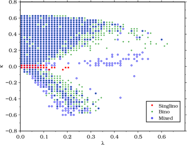
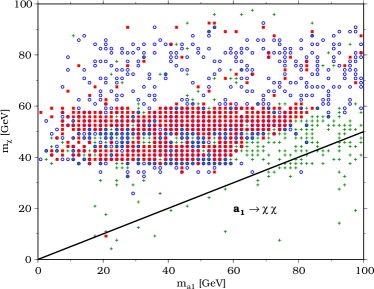
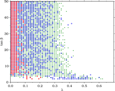
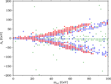
Figure 1: The allowed region of $(\lambda-\kappa)$ parameter space (upper-left); the $m_{\widetilde{\chi}_{1}^{0}}$ vs. $m_{a_{1}}$ plane (upper-right)– the decay $a_{1}\rightarrow{\widetilde{\chi}_{1}^{0}}{\widetilde{\chi}_{1}^{0}}$ is allowed for those models below the line; the $(\tan\beta-\lambda)$ viable parameter space (lower-left); $A_{\kappa}$ as a function of the lightest CP-odd Higgs mass (lower-right)

As can be seen from Fig. 1, the neutralino is mostly a singlino when $\kappa$ and $\lambda$ are small. We can understand this feature by realizing that the upper $4\times 4$ block in the neutralino mass matrix, Eq. (5), corresponds to the MSSM. From the lower $3\times 3$ block it can be appreciated that the singlino decouples from the MSSM part when Franke:2001nx :

$$2|\kappa s|,\>\lambda v<M_{1},\>M_{2},\>|\mu|.$$ (8)

It must be stressed that our Fig. 1 shows only models which give an acceptable relic density. This might explain the absence of singlino-like neutralinos at moderate $\lambda\sim 0.3$.

A CP-odd Higgs so light that the decay $a_{1}\rightarrow{\widetilde{\chi}_{1}^{0}}{\widetilde{\chi}_{1}^{0}}$ is possible, is generally not viable for light singlino-like neutralinos. This makes them cosmologically disfavored, since this resonant decay is required to enhance the annihilation cross-section and obtain the correct relic density. A nearly complete mass degeneracy between ${\widetilde{\chi}_{1}^{0}}$ and either the next-to-lightest neutralino, $\widetilde{\chi}_{2}^{0}$, or the lightest chargino, suppressing the LSP final relic abundance through large coannihilation effects, usually occurs for the viable light singlino models Belanger:2006is .

We can see from Fig. 1 that singlino models at large $\lambda$ feature small $\tan\beta\lesssim 5$, since large values of $\tan\beta$ induce sizable singlino mixing. We also expect models with moderate $\tan\beta$, for which annihilation through a Higgs resonance is marginal in the MSSM, to be peculiar of the NMSSM setup.

Finally, the lower-right panel in Fig. 1 shows how a light CP-odd Higgs boson, $a_{1}$, appears when $A_{\kappa}\rightarrow 0$. We stress that this regime, when the $U(1)_{R}$ symmetry approximately holds, is well motivated in the context of gaugino mediated Susy breaking Chacko:1999mi where $A_{\kappa}$ is only generated at the two loop level.

III NMSSM Dark Matter Indirect detection

Neutralinos, being weakly interacting and electrically neutral particles are very difficult to observe in collider experiments directly. If they make up a sizable fraction of the galactic halo dark matter, however, other methods of detection become feasible Bertone:2004pz ; Jungman:1995df .

Monitoring the energy deposited as they scatter off nuclei in detectors falls into the realm of direct detection methods. A group of experiments is actively exploring this path, although, as already mentioned, their sensitivity decreases for neutralinos below $m_{\chi}\lesssim 100\ {\rm GeV}$. The prospects for direct detection of NMSSM neutralinos have already been discussed in the literature Bednyakov:1998is ; Cerdeno:2004xw ; Gunion:2005rw .

We focus here on the possibility that dark matter neutralinos can be detected by looking at products of their pair annihilation. Chief among them are neutrinos, photons and antiparticles Bertone:2004pz ; Jungman:1995df ; Feng:2000zu ; Zeldovich:1980st .

Neutrino fluxes from neutralino annihilations are searched for in underground neutrino telescopes. Present facilities such as Super-Kamiokande and MACRO, with low energy thresholds, $E_{\nu}\gtrsim 1\ {\rm GeV}$, are particularly useful to constrain the light NMSSM dark matter particles that we consider. Some of the planned facilities (e.g. AMANDA, ICECUBE) are geared to detecting neutrinos above $100\ {\rm GeV}$, and we don’t consider them here. ANTARES, on the other hand, promises to improve the sensitivity to moderately energetic neutrinos by an order of magnitude and will be of importance for our discussion.

Gamma-rays are also produced in neutralino annihilations. They can be detected by earth-based Cherenkov telescopes (MAGIC, HESS, VERITAS, …) or in space-borne facilities (EGRET, GLAST, AMS), although, only the latter have the ability to observe the low energy photons from light neutralinos such as those considered here.

Other satellites, like PAMELA, GAPS and AMS, will measure the flux of antiparticles and antimatter nuclei.

We study below the signatures of light NMSSM dark matter particles in neutrino telescopes, gamma-ray satellites and antimatter detectors. We also touch upon the effects on the Sun caused by neutralino energy transport.

The main ingredient for indirect detection prediction are the different annihilation modes of neutralinos. Since dark matter in the halo moves at non-relativistic velocities, $v\sim 10^{-3}c$, only the channels with a CP-odd final state can occur. The branching ratios for the relevant tree level processes are reviewed in App. A, together with the most important one loop channels.

Neutrino fluxes from neutralino annihilations are enhanced in the direction of the center of the Sun or of the Earth. The abundance of neutralinos trapped within these objects depends on the scattering cross sections of neutralinos with nuclei that can be found in App. B.

We start our discussion by studying the information that can be gained from the observation of neutrino fluxes.

III.1 Neutrino Fluxes from Neutralino annihilations in the Earth and in the Sun

The observation of energetic neutrinos from annihilation of neutralinos in the Sun Silk:1985ax ; Krauss:1985ks and/or the Earth Krauss:1985aa ; Freese:1985qw , is a promising method for indirect detection of neutralino dark matter (see e.g. Bertone:2004pz ; Jungman:1995df for a review).

Neutralinos making up the dark matter in the halo of the Galaxy have a small but finite probability of elastically scattering from a nucleus in a given body (the Sun or the Earth). In doing so, neutralinos might be left with a velocity smaller than the escape velocity and, thus, become gravitationally bound to the body. The captured neutralinos settle to the core of the body, via additional scatterings from nuclei in the body, and eventually annihilate with one another.

The pair annihilation of the accumulated neutralinos generates, via decay of the particles produced in the various annihilation final states, high energy neutrinos with a differential flux given by:

$$\frac{dN_{\nu}}{dE_{\nu}}=\frac{\Gamma_{ann}}{4\pi d^{2}}\sum_{f}{BR_{f}\frac{dN_{f}}{dE}}$$ (9)

Here $d$ is the distance of the detector from the Sun or the center of the Earth, $\Gamma_{ann}$ is the annihilation rate of the neutralinos, $BR_{f}$ is their branching ratio into the final state $\chi\chi\rightarrow f$ and $dN_{f}/dE$ is the neutrino spectrum from the decay of the particles in the final state $f$.

Since neutralinos inside the Sun or the Earth are highly non-relativistic, their annihilations occur almost at rest. The branching ratios of the different annihilation channels are discussed in App. A.

A light neutralino can only annihilate into the light quarks and lepton pairs, which, after decay, give rise to a fairly soft neutralino spectrum. A more massive $\chi$ can lead to $W^{+}W^{-}$, $ZZ$ and heavier quark pairs, which typically produce a harder differential neutralino flux. Apart from these fundamental channels, neutralino annihilations can produce Higgs bosons or mixed Higgs/gauge boson final states. The Higgs bosons will, in turn, decay to other Higgses or to one of the “fundamental” channels Ritz:1987mh . In our calculations, we have taken into account the fact that the number of final states containing Higgs bosons is increased in the NMSSM due to the extra CP-even and CP-odd states, $h_{3}$ and $a_{2}$, compared to the MSSM.

III.1.1 Annihilation rate in the Sun and in the Earth

Neutralinos accumulate in the Sun or the Earth by capture from the halo of the Galaxy, and are depleted by annihilation and by evaporation. The evolution equation for the number of neutralinos, $N$, in the Sun or the Earth is given by:

$$\frac{dN}{dt}=C-C_{A}N^{2}-C_{E}N$$ (10)

where $C$ is the rate of accretion onto the body, the second term is twice the annihilation rate and the last term accounts for neutralino evaporation.

Evaporation has been shown to be important only for neutralinos lighter than $3-5\>{\rm GeV}$ Griest:1986yu ; Gould:1987ju . The lightest neutralino that we consider in this paper is on the upper range, $m_{\chi}\sim 5\>{\rm GeV}$, so we can safely neglect the last term in Eq. (10).

We then solve Eq. (10) for $N$, and obtain the annihilation rate at any given time:

$$\Gamma_{ann}=\frac{C}{2}{\rm tanh}^{2}\left(t/\tau_{A}\right)$$ (11)

where $\tau_{A}=1/\sqrt{CC_{A}}$ is the time scale for capture and annihilation equilibrium to occur. We will be interested in the value of $\Gamma_{ann}$ today, for $t=t_{\odot}\simeq 1.5\times 10^{17}\>{\rm s}$.

The annihilation rate per effective volume, $C_{A}$ is given by:

$$C_{A}=\left<\sigma_{A}v\right>\frac{V_{2}}{V_{1}^{2}},$$ (12)

and $V_{j}=\left[3m_{Pl}^{2}T/(2jm_{\chi}\rho)\right]^{3/2}$ are the effective volumes for the Sun ($V_{j}\sim 6.6\times 10^{28}(jm_{\chi,10})^{-3/2}\>{\rm cm}^{3}$) or the Earth ($V_{j}\sim 2.3\times 10^{25}(jm_{\chi,10})^{-3/2}\>{\rm cm}^{3}$).

The total annihilation rate, $\left<\sigma_{A}v\right>$, is calculated with all the contributions at tree level, with the inclusion of the of the two gluon channel discussed in App. A.

The accretion rate in the Sun was first calculated in Krauss:1985ks and  Press:1985ug , and for the Earth in Freese:1985qw ; Krauss:1985aa . More detailed evaluations can be found in Gould:1987ir . The results depend on the velocity dispersion in the halo, the velocity of the Sun with respect to the halo, the local density of dark matter and the composition of the Sun or the Earth. For the Sun, we use the analytic approximations to the results of Gould:1987ir that can be found in Jungman:1995df , and the solar model we use is that of Bahcall:2000nu , with additional abundances taken from Grevesse:1998bj . For the Earth, we follow Gould:1987ir .

The capture rate of neutralinos inside the Earth receives an additional contribution from a subpopulation of neutralinos that scatter on a nucleus located near the surface of the Sun, and lose enough energy to stay in Earth-crossing orbits which, due to planetary perturbations, do not intersect with the Sun Damour:1998rh . This addition to the local density of dark matter in the Earth has a characteristic velocity that more closely matches the escape velocity from the Earth than the background halo population, enhancing the resonant capture off elements such as iron. This effect is more important for the light, $m_{\chi}\lesssim 100\>{\rm GeV}$, neutralinos that we are considering and we thus take it into account when computing capture rates in the Earth.

The capture of neutralinos in the Sun or the Earth depends on the elastic scattering cross sections with the nuclei that make up the body. These cross sections can be derived Jungman:1995df from the nucleon (proton or neutron) cross sections that are discussed, for the NMSSM, in App. B. We have included both spin-independent and spin-dependent terms in our computations, the latter being potentially important to evaluate the accretion in the Sun.

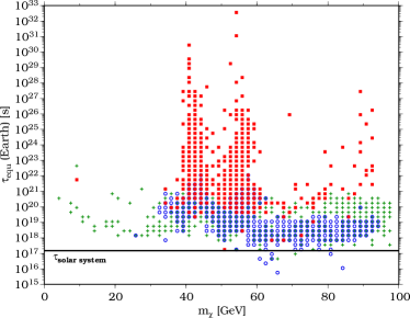
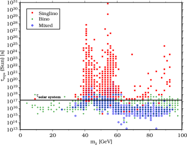
Figure 2: Equilibrium times between capture and annihilation in the Earth (left) and the Sun (right). Models below the line marking the age of the solar system have attained equilibrium and will have an $\Gamma_{ann}\sim C/2$

We show in Fig. 2 the equilibrium time between capture and annihilation in the Earth and in the Sun. Most bino and mixed-like neutralinos have reached equilibrium and ${\rm tanh}^{2}\left(t_{\odot}/\tau_{A}\right)\sim 1$ in Eq. (11). In the Earth, featuring a shallower gravitational potential well, equilibrium has only been reached by a few mixed-like neutralinos, and the annihilation rate will be below $C/2$. The emission region is however much closer to the detector, and, as we will see below, and in contrast to the usual situation in the MSSM, the constraints from the Earth are more stringent than those from the Sun.

III.1.2 Muon fluxes

The neutralino annihilation products will hadronize and/or decay giving rise to high energy neutrinos, $E_{\nu}\lesssim m_{\chi}$, which may be detected in a neutrino telescope by measuring the upward-going muons produced by $\nu_{\mu}$ and $\bar{\nu}_{\mu}$ interactions in the rock below the detector.

The precise determination of the secondary neutrino spectrum is a difficult problem that calls for dedicated Monte Carlo simulations of the hadronization and energy losses in the medium of the body. We have used the results of Bergstrom:1996kp and adapted the relevant routines in DarkSUSY Gondolo:2004sc , to take into account the additional Higgses present in the NMSSM. Spectra are given for six fundamental channels, $\chi\chi\rightarrow c\bar{c},\>b\bar{b},\>t\bar{t},\>\tau\bar{\tau},\>W^{+}W^{-},\>ZZ$, which are also used for the Higgs and Higgs/gauge boson final states by following the decay chain until one of the fundamental channels is reached.

The muon yields in Bergstrom:1996kp include the effects of hadronization/decay of the annihilation products, $\nu$ interactions on their way out of the Sun and near the detector, and of the multiple Coulomb scattering of the $\mu$ on its way to the detector. A similar study was done in Bottino:1994xp .

The effects of oscillations in the propagation of the neutrinos through the Sun have been discussed in Roulet:1995qb . More recently, the full spectra of all neutrino flavors including additional channels, such as light quarks and gluons, and accounting for oscillations and $\nu_{\tau}$-regeneration were given in Cirelli:2005gh . The combined effect amounts to a ${\cal O}(0.1-10)$ correction which is comparable to astrophysical uncertainties. We do not include these effects here, although if an anomalous $\nu$ signal were discovered, it would be then interesting to try to reconstruct the mass and branching ratios of the would-be neutralinos Cirelli:2005gh .

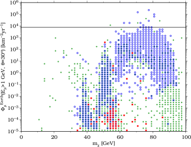
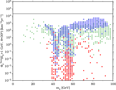
Figure 3: Integrated muon fluxes above $E_{\mu}\geq 1{\rm GeV}$ from the Earth (left) and the Sun (right). The horizontal line displays the MACRO bound Ambrosio:1998qj .

Fig. 3 shows the muon fluxes for $\chi\chi$ annihilation from the Earth and from the Sun. We show integrated fluxes above a threshold energy of $1\>{\rm GeV}$ and the horizontal line represents the MACRO limit Ambrosio:1998qj which is comparable to that of Super-Kamiokande Desai:2004pq . To be able to constrain the low mass neutralinos considered in this work, it is crucial for the detector to have a low threshold. Of all the forthcoming facilities, ANTARES Aguilar:2003us seems to be the most promising one, with an advertised threshold of $E_{\mu}\sim 10\>{\rm GeV}$ and a target sensitivity of $100-1000\>{\rm km}^{-2}{\rm yr}^{-1}$, it should be able to detect or further constrain those models with $m_{\chi}\gtrsim 20\>{\rm GeV}$. Larger facilities like ICECUBE Achterberg:2006md have sparser instrumentation, which increases the threshold to $E_{\mu}\gtrsim 100\>{\rm GeV}$, above the mass range in which we are interested.

In Fig. 3, we considered a half-aperture of $\theta=30^{\circ}$. A cone of this size should contain most of the muons from annihilations of even the lightest neutralinos. For moderately larger masses, a smaller aperture could improve the signal to noise ratio by reducing the background while still collecting most of the signal, and the limits could be improved by an optimized analysis.

It is encouraging, however, that present muon fluxes due to capture in the Earth, presumably in part due to the enhancement in the density of light neutralinos in solar system orbits, are currently able to rule out a few models with moderate masses, $m_{\chi}\sim 60-80\>{\rm GeV}$, and that an order of magnitude improvement in sensitivity as expected with the ANTARES telescope, should enable to access a sizable part of the parameter space by looking at signals from both the Sun and the Earth. On the other hand, singlino-like neutralinos show suppressed muon fluxes and prospects for their detection seem more remote.

III.2 Solar Physics Bounds

Energy transport by neutralinos could have relevant effects on the Sun, producing an isothermal core and reducing the Sun central temperature, $T_{c}$. WIMPs with masses of a few ${\rm GeV}$ and elastic scattering cross-sections around $\sigma_{el}\sim 10^{-36}\>{\rm cm}^{2}$, were considered some time ago as being able to reduce the solar neutrino flux, hence solving the solar neutrino problem  Krauss:1984a ; Spergel:1984re ; Krauss:1985ks ; Faulkner:1985rm . It has, since then, been realized that the solar neutrino problem cannot be solved by simply reducing $T_{c}$, and this hypothesis was abandoned.

On the other hand, our knowledge of the solar interior has advanced to a point where stellar evolution theory in combination with observational data could provide information on the existence and properties of the particles constituting the dark matter. The sound speed in the Sun is known with an accuracy of roughly $0.1\%$ through helioseismic data Degl'Innocenti:1996ev , and the measurement of the neutrino flux from ${}^{8}B$ decay has enabled the determination of $T_{c}$ at the percent level Fiorentini:2001et .

The variations in the sound speed induced by dark matter particles were considered in Lopes:2001ra and, together with the influence on the boron neutrino flux Lopes:2001ig , were claimed to exclude WIMPs below $m_{\chi}\lesssim 60\>{\rm GeV}$. This stringent conclusions were due, according to Bottino:2002pd , to an unrealistic extrapolation of the helioseismic data down to the central regions of the Sun. Neutralinos as light as $m_{\chi}\sim 30\>{\rm GeV}$ were shown to be in accord with helioseismology and also to leave the neutrino fluxes unchanged, since the central temperature was only being modified in a small region around the center of the Sun.

It is nonetheless of interest to consider the influence on the solar energy transport of neutralinos within the NMSSM. Apart from changes in the capture rates, the mass of the neutralinos we are considering here dwell well below $m_{\chi}\sim 30\>{\rm GeV}$, creating a larger isothermal core with potential observable effects.

Energy transport in the Sun can occur by diffusion or in a non-local manner. The prevalence of either regime is determined by the Knudsen number, which is the ratio of the mean free path of the weakly interacting neutralino in the multicomponent baryonic background to the scale length of the system:

$$Kn\equiv\left(L\sum_{i}{\sigma_{i}n_{i}}\right)^{-1},$$ (13)

where the sum runs over the chemical elements in the Sun.

For neutralinos in the Sun, the relevant geometric dimension is the scale height of the neutralino cloud in the central region, which can be approximated by:

$$L=r_{\chi}\sim 0.13R_{\odot}\sqrt{\frac{1\>{\rm GeV}}{m_{\chi}}}.$$ (14)

When the mean free path is short compared to $r_{\chi}$, energy is transported by thermal conduction and the relevant Boltzmann collision equation has been carefully studied in Gould:1989hm . We will be mostly interested in the opposite regime, the Knudsen limit, when $Kn\gg 1$ and the particles orbit many times in the Sun between interactions with nuclei. An analytic approximation for this case was presented in Spergel:1984re , although Monte Carlo simulations Nauenberg:1986em revealed that it overestimated the neutralino luminosity by a factor of a few. This was subsequently confirmed, and the source of the discrepancy attributed to the deviation from isotropy of the neutralino distribution Gould:1989ez . With this caveat in mind, it will suffice, for our purposes, to estimate the neutralino luminosity using the results of Spergel:1984re .

We asserted above that the neutralinos will be transferring energy in the Knudsen regime: let us show now that this is indeed the case. The critical cross section for an interaction to occur in a solar radius can be estimated as:

$$\sigma_{c}\sim\frac{m_{p}}{M_{\odot}}R_{\odot}^{2}\sim 4\times 10^{-36}{\rm cm}^{2}$$ (15)

The $\chi-n,p$ elastic scattering cross sections that we obtain using the results in App. B fall a few orders of magnitude below $\sigma_{c}$. For some mixed-like neutralinos we get values as large as $2\times 10^{-39}\ {\rm cm}^{2}$, an order of magnitude larger than for bino-like neutralinos and some three orders of magnitude above those of singlinos. Hence, the neutralinos will travel over distances larger than $10^{3}R_{\odot}$, corresponding to Knudsen parameters in the range $Kn\gtrsim 10^{3}$. We show the parameter in Fig. 4 at a distance $r_{\chi}$ from the center of the Sun, which is where the neutralino luminosity is expected to peak Gould:1989ez .

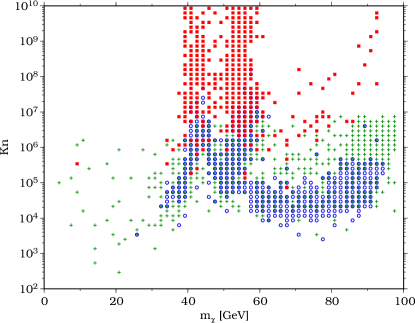
Figure 4: Knudsen number, Eq. (13), at a distance $r_{\chi}$

.

The energy transport is most effective in the region $Kn\sim 0.4$ Gould:1989hm ; Gould:1989ez , far below the values depicted in Fig. 4, so we expect the neutralino luminosity to be a fraction of the total solar luminosity ${\cal L}_{\odot}$. Indeed, we can obtain a rough estimate of ${\cal L}_{\chi}$, by adapting Eqs. (2.8-2.10) in Spergel:1984re to account for the different species of nuclei in the Sun, and assuming the neutralino luminosity is confined to a region of size $r_{\chi}$:

$${\cal L}_{\chi}\sim\frac{N_{\chi}R_{\odot}^{2}\sigma_{c}}{r_{\chi}^{4}Kn}\sqrt{\frac{1\>{\rm GeV}}{m_{\chi}}}4.1\times 10^{12}{\cal L}_{\odot},$$ (16)

where the number of neutralinos in the Sun is given by $N_{\chi}=C\tau_{A}{\rm tanh}(t_{\odot}/\tau_{A})$.

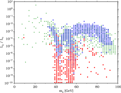
Figure 5: Neutralino luminosity in units of ${\cal L}_{\odot}$.

Looking at Fig. 5, where we see that most models contribute a tiny fraction of the solar luminosity. However for the lightest bino-like neutralinos, $m_{\chi}\lesssim 30\ {\rm GeV}$, the neutralino luminosity may be comparable to the total solar luminosity, and may thus already be disfavored.

We have already mentioned that the neutralino luminosity might be overestimated by a factor of ${\cal O}(10)$. On the other hand, the neutralino luminosity is not directly observable, and it is not unconceivable that neutralinos giving a smallish fraction of the total luminosity, but having a small mass and, hence, a sizable isothermal core, might modify the boron neutrino fluxes appreciably. As pointed out in Spergel:1984re , a $20\ {\rm GeV}$ neutralino carrying only $10^{-2}{\cal L}_{\odot}$, could be responsible for the transfer of up to $50\%$ of the energy in the inner region bounded by $r_{\chi}$. Computing the actual modifications in neutrino fluxes and/or helioseismic data, would require the generation of self-consistent solar models with the neutralino transport taken into account. Although this is beyond the scope of the present work, the present estimates suggest that this task may deserve further investigation for light NMSSM neutralinos.

III.3 Antimatter from Neutralino annihilations in the Galactic Halo

Neutralino pair-annihilations in the galactic halo can produce, through the hadronization or decay of the underlying elementary constituents arising from the annihilation process, antimatter in the form of positrons and of hadronic stable antimatter states like antiprotons and antideuterons. The abundance of antimatter fluxes produced in neutralino pair-annihilations not only depends upon the particle physics nature of neutralinos, but also on various astrophysical factors. The latter–including the structure of the dark matter galactic halo, the propagation of cosmic rays in the Galaxy, the effects of solar modulation–induce some amount of uncertainty in the flux computation. Further, while in the case of low-energy antideuterons the cosmic ray background can be suppressed at a level where the detection of even a single antideuteron can be a signal for new physics and potentially for dark matter annihilations in the halo, for positrons and antiprotons the background is large. While this latter background is, to some extent, understood, it has to be properly incorporated and estimated if one is to be able to extract a possible dark matter annihilation signal from the data.

As far as the dark matter distribution in the galactic halo is concerned, we resort here to the strategy outlined in Ref. Profumo:2004ty (the reader is referred to Ref. pierohalos ; Edsjo:2004pf ; Profumo:2004at for more details). We consider two extreme possibilities for the structure of the dark matter halo. In the first scenario, the central cusp in the dark matter halo, as seen in numerical simulations, is smoothed out by a significant heating of the cold particles elzant , leading to a cored density distribution, which has been modeled by the so called Burkert profile burkert ,

$$\rho_{B}(r)=\frac{\rho_{B}^{0}}{(1+r/a)\left(1+(r/a)^{2}\right)}.$$ (17)

Here, the length scale parameter has been set to $a=11.7$ kpc, while the normalization $\rho_{B}^{0}$ is adjusted to reproduce the local halo density at the Earth position to $\rho_{B}(r_{0})=0.34\ {\rm GeV\ cm}^{-3}$ pierohalos . We refer to this model as to the Burkert Halo Model. It has been successfully tested against a large sample of rotation curves of spiral galaxies salucci .

In the second scenario we consider here, baryon infall causes a progressive deepening of the gravitational potential well at the center of the galaxy, resulting in an increasingly higher concentration of dark matter particles. In the circular orbit approximation blumental ; ulliobh , this adiabatic contraction limit has been worked out starting from the N03 profile proposed in Ref. n03 ; the resulting spherical profile, which has no closed analytical form, roughly follows, in the inner galactic regions, the behavior of the profile proposed by Moore et al.,moore , approximately scaling as $r^{-1.5}$ in the innermost regions, and features a local dark matter density $\rho_{N03}(r_{0})=0.38\ {\rm GeV\ cm}^{-3}$. We dub this setup as the Adiabatically Contracted N03 Halo Model.

The parameters for both models have been chosen to reproduce a variety of dynamical information, ranging from the constraints stemming from the motion of stars in the sun’s neighborhood, total mass estimates from the motion of the outer satellites, and consistency with the Milky Way rotation curve and measures of the optical depth toward the galactic bulge pierohalos ; Edsjo:2004pf . Both models have been included in the latest public release of the DarkSUSYpackage Gondolo:2004sc .

The antimatter yields from neutralino annihilation are then computed following the procedure outlined in Ref. Profumo:2004ty . We calculate the neutralino annihilation rates to $\bar{p}$ and $\bar{n}$ using the Pythia 6.154 Monte Carlo code pythia as implemented in DarkSUSY Gondolo:2004sc , and then deduce the $\overline{D}$ yield using the prescription suggested in Ref. dbar . The propagation of charged cosmic rays through the galactic magnetic fields is worked out through an effective two-dimensional diffusion model in the steady state approximation Bergstrom:1999jc , while solar modulation effects were implemented through the analytical force-field approximation of Gleeson and Axford GleesonAxford . The solar modulation parameter $\Phi_{F}$ is computed from the proton cosmic-ray fluxes, and assumed to be charge-independent. The values of $\Phi_{F}$ we make use of refer to a putative average of the solar activity over the three years of data taking of the recently launched Payload for Antimatter Matter Exploration and Light-nuclei Astrophysics (PAMELA) experiment pamelanew for positrons and antiprotons, and over the estimated period of data-taking for the General Anti-Particle Spectrometer (GAPS) experiment in the case of antideuterons.

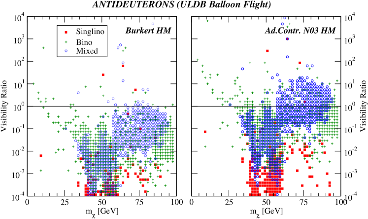
Figure 6: The expected number of antideuterons detectable with an ultra-long duration balloon-borne GAPS-type experiment, as a function of the lightest neutralino mass. In the left panel we adopt a Burkert halo model, while in the right panel we make use of an adiabatically contracted N03 halo profile. The conventions for the various neutralino types follow those of Fig. 1.

For antideuterons we consider the reach of the proposed general antiparticle spectrometer (GAPS) Mori:2001dv ; gapsnew in an ultra-long duration balloon-borne (ULDB) mission, tuned to look for antideuterons in the very low kinetic energy interval from 0.1 to 0.25 GeV per nucleon. As described in Ref. dbarprofumo , in fact, this experimental setting would allow one to safely neglect the background from secondary and tertiary cosmic-ray-produced antideuterons, unlike a satellite-borne mission: the detection of a single low-energy antideuteron would then be a clean signature of an exotic antideuteron source (including, but not limited to, galactic dark matter annihilation). We set the value of the solar modulation parameter $\Phi_{F}$ at the value corresponding to the projected year for the balloon-borne GAPS mission, around 2011. The resulting sensitivity of GAPS has been determined to be of the level of $3\times 10^{-8}{\rm m}^{-2}{\rm sr}^{-1}{\rm GeV}^{-1}{\rm s}^{-1}$  gapsnew ; dbarprofumo .

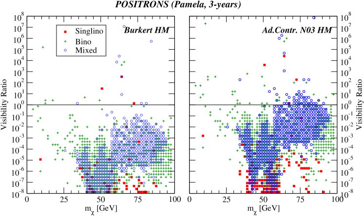
Figure 7: The Visibility Ratio for positrons, as defined in Eq. (21), as a function of the lightest neutralino mass. In the left panel we adopt a Burkert halo model, while in the right panel we make use of an adiabatically contracted N03 halo profile. The conventions for the various neutralino types are as in Fig. 1.

To evaluate the sensitivity of the PAMELA antimatter search experiment, we adopt the statistical treatment of the antimatter yields introduced in Ref. Profumo:2004ty (an analogous approach has been proposed for cosmic positron searches  Hooper:2004bq ). Motivated by the fact that the signal is much smaller than the background, we introduce a quantity which weighs the signal’s “statistical significance, summed over the energy bins”,

$$I_{\phi}=\int_{T_{\rm min}}^{T_{\rm max}}\frac{\left(\phi_{s}(E)\right)^{2}}{\phi_{b}(E)}{\rm d}E,$$ (18)

where $\phi_{s}(E)$ and $\phi_{b}(E)$ respectively represent the antimatter differential fluxes from neutralino annihilations and from the background at antiparticles’ kinetic energy $E$, and $T_{\rm min,\ max}$ correspond to the antiparticle’s maximal and minimal kinetic energies to which a given experiment is sensitive (in the case of the PAMELA experiment pamelanew , $T^{e^{+}}_{\rm min}=50$ MeV, $T^{e^{+}}_{\rm max}=270$ GeV, $T^{\bar{p}}_{\rm min}=80$ MeV and $T^{\bar{p}}_{\rm max}=190$ GeV). It can be easily verified that Eq. (18) reproduces, in the large-number-of-bins limit, the excess $\chi^{2}$ from an exotic contribution in the fit to the prospect antimatter fluxes. We compute the primary component, $\phi_{s}$, with the DarkSUSYpackage, interfaced with a subroutine implementing the diffusion and solar modulation models outlined above. The background flux $\phi_{b}$ has been calculated with the Galprop package galprop , with the same propagation and solar modulation parameter choices employed to compute the signal.

Given an experimental facility with a geometrical factor (acceptance) $A$ and a total data-taking time $T$, it has been shown Profumo:2004ty that, in the limit of a large number of energy bins and of high precision secondary (i.e. background) flux determination, a SUSY model giving a primary antimatter flux $\phi_{s}$ can be discriminated at the 95% C.L. if

$$I_{\phi}(\phi_{s})\cdot A\cdot T>(\chi^{2})^{95\%}_{\rm n_{b}},$$ (19)

where $(\chi^{2})^{95\%}_{\rm n_{b}}$ stands for the 95% C.L. $\chi^{2}$ with ${\rm n_{b}}$ degrees of freedom. For the PAMELA experiment, where $A=24.5\ {\rm cm}^{2}\ {\rm sr}$, $T$=3 years and ${\rm n_{b}}\simeq 60$ we get the following discrimination condition Profumo:2004ty

$$I_{\phi}(\phi_{s})>\frac{(\chi^{2})^{95\%}_{\rm n_{b}}}{A\cdot T}\equiv I_{\phi}^{\rm 3y,\ PAMELA,\ 95\%}\simeq 3.2\times 10^{-8}\ {\rm cm}^{-2}{\rm sr}^{-1}{\rm s}^{-1}$$ (20)

which is approximately valid for both positrons and antiprotons (though in the latter case the PAMELA experiment is expected to do slightly better). As a rule of thumb, the analogous quantity for AMS-02 should improve at least by one order of magnitude Feng:2000zu . In our plots, we will show, for both antiprotons and positrons, the following “Visibility Ratio”

$${\rm Visibility\ Ratio}\equiv I_{\phi}^{\bar{p},e^{+}}/I_{\phi}^{\rm 3y,\ PAMELA,\ 95\%}.$$ (21)

We show our results on the prospects for detecting a WIMP pair annihilation signature in the various above mentioned antimatter channels in Fig. 6-8. As in the previous figures, we indicate singlino-like models with red squares, bino-like with green pluses and mixed singlino-bino models with empty blue circles. Models lying above the horizontal lines are expected to give a detectable signature at the experiments discussed above. In all three figures, we adopt the Burkert Halo Model in the left panels and the adiabatically contracted N03 Halo Model in the right panels. As a general comment, switching from the conservative Burkert profile to the more optimistic adiabatically contracted halo profile causes an increase in the fluxes of around one order of magnitude (notice that, in terms of the Visibility Ratio, Eq. (21), for antiprotons and positrons, which depends on the square of the signal flux, this translates into a two orders of magnitude increase).

Figure 8: The Visibility Ratio for antiprotons, as defined in Eq. (21), as a function of the lightest neutralino mass. In the left panel we adopt a Burkert halo model, while in the right panel we make use of an adiabatically contracted N03 halo profile. The conventions for the various neutralino types are as in Fig. 1.

We start showing, in Fig. 6, the Visibility Ratio for antideuterons, effectively given by the expected number of detected antideuterons at an ULDB GAPS mission. As alluded above, this experimental setup is virtually devoid of cosmic ray background, hence the detection of even only one $\bar{D}$ can be regarded as a “signal”. We notice that in general, low mass neutralinos, peculiar of the NMSSM setup under consideration here, yield a sizable flux of low-energy antideuterons. With some exceptions, singlino-like neutralinos produce an insufficient flux of $\bar{D}$, while the most promising models are mixed singlino-bino models with a mass in the range $55\lesssim m_{\chi}/{\rm GeV}\lesssim 95$.

Fig. 7 and 8 respectively show the Visibility Ratios for positrons and for antiprotons. As a general comment, we point out that in the present setup antiprotons stand as a more promising channel to effectively disentangle an exotic signal. As for the case of antideuterons, low mass models are again expected to give a sizable antimatter yield. While we do find some instances of singlino-like neutralinos that can give large antimatter fluxes, in general we find that the antiproton and positron yield from singlinos is not particularly promising. On the other hand, mixed models, peculiar to the NMSSM, give in general large fluxes, and a significant portion of the models will be tested by the results from the space-based PAMELA experiment on a time scale of three years (or by AMS-02 in a much shorter time scale).

We also computed the constraints from current antiproton currpbar and positron curreplus flux measurements, in terms of the $\chi^{2}$ to the data of the sum of the background and the signal. Using this criterion, we find that models featuring an antiproton Visibility Ratio larger than $\sim 10$ are generically conflicting with current data, and so are models giving a positron Visibility Ratio larger than $\sim 300$. However, one should keep in mind that the background we use in our computation can be somewhat lowered without conflicting with cosmic ray propagation models; in a more conservative approach, asking that the signal alone does not exceed the measured antiproton flux, rules out only models with Visibility Ratios larger than $\sim 100$ ($\sim 1000$ in the case of positrons).

III.4 The Monochromatic Gamma-ray Flux

Neutralinos can pair annihilate in the Galaxy or in dark matter concentrations outside the Galaxy yielding a coherent and directional flux of gamma rays; two components add up in the total gamma-ray yield expected from neutralino pair-annihilations: a continuum part, extending up to gamma-ray energies $E_{\gamma}\lesssim m_{\chi}$, generated by annihilation products radiation and from decays of, e.g., $\pi^{0}\rightarrow\gamma\gamma$, and (possibly more than one) monochromatic lines, in loop-induced direct decays to, e.g., $\gamma\gamma$, $Z\gamma$ or $H\gamma$ final states. Among the latter, the brightest, and the one which occurs in any supersymmetric framework (the others being potentially kinematically forbidden) is often that associated to the $\gamma\gamma$ final state. Since the possibility of unambiguously disentangling the continuum gamma-ray contribution from the background is known to be observationally extremely challenging (see e.g. the recent analyses in Ref. gammaraysref1 ; gammaraysref2 ; Zaharijas:2006qb ), and in view of our expectations on the size of the $\gamma\gamma$ annihilation channel in the NMSSM, as anticipated in the Introduction, we shall concentrate here on the monochromatic gamma-ray line from radiative annihilation of neutralinos into two photons, at an energy $E_{\gamma}=m_{\chi}$.

As well known, the estimate of the gamma-ray flux from WIMP pair annihilation critically depends upon the assumptions one makes on the dark matter profile in the inner portions of the halos. This spread can be extremely large in the case of the nearby Galactic Center, where the dark matter distribution is poorly constrained by observational data. One is then forced to extrapolate the assumed dark matter profile to very small regions around the center of the Galaxy; the small scale central structure of dark matter halos plays, instead, a less crucial role when the source is located further away gammaraysref1 , as in the case of nearby dwarf satellite galaxies gammaraysref1 ; draco ; Colafrancesco:2006he or of galaxy clusters Colafrancesco:2005ji . A second issue involved in the evaluation of the possibility of detecting a WIMP annihilation signal in gamma-ray data is related to the evaluation of the background. In short, any evaluation of the detectability of a WIMP induced gamma-ray signal must be carefully and properly put in a specific context; comparing the detection perspectives for different astrophysical WIMP annihilation locations can be even more difficult, and full details about the assumptions involved have to be specified.

In Fig. 9 we compare the detection prospects, in the $(m_{\chi},\langle\sigma v\rangle_{\gamma\gamma})$ plane (where $\langle\sigma v\rangle_{\gamma\gamma}\equiv\langle\sigma v\rangle\times{\rm BR}(\chi\chi\rightarrow\gamma\gamma)$), of the $\gamma\gamma$ line from neutralino pair-annihilations in the Galactic Center (left) and in the Draco dwarf spheroidal galaxy (right) with the predictions we obtain in our scan over NMSSM models. We consider the sensitivity of GLAST after five years of data taking time $T$, assuming an average angular sensitivity of $\Delta\Omega\simeq 9\times 10^{-5}$ sr, and an average effective area $A_{\rm eff}$ of 5000 cm² glastsens . We consider a putative energy bin centered around the location of the gamma-ray line, $E_{\gamma}=m_{\chi}$, and as wide as the expected energy resolution of GLAST, $\Delta E/E\simeq 0.1$. Namely, we consider the energy interval

$$(\Delta E)_{m_{\chi}}\equiv m_{\chi}/1.05\lesssim E_{\gamma}\lesssim m_{\chi}\times 1.05.$$ (22)

Given a background with a differential flux

$$\frac{{\rm d}\phi_{b}}{{\rm d}E}\simeq\phi_{0}\left(\frac{E}{1\ {\rm GeV}}\right)^{-\gamma}$$ (23)

we obtain, over the considered energy range a total background flux of

$$\phi_{b}=\frac{\phi_{0}}{\gamma-1}\left(\left(\frac{m_{\chi}/1.05}{1\ {\rm GeV}}\right)^{1-\gamma}-\left(\frac{m_{\chi}\times 1.05}{1\ {\rm GeV}}\right)^{1-\gamma}\right)\ {\rm cm}^{-2}{\rm s}^{-1}.$$ (24)

The signal flux from the monochromatic line is instead given by

$$\phi_{s}=1.87\times 10^{-11}\left(\frac{2\times\langle\sigma v\rangle_{\gamma\gamma}}{10^{-29}\ {\rm cm}^{3}{\rm s}^{-1}}\right)\left(\frac{10\ {\rm GeV}}{m_{\chi}}\right)^{2}\cdot\overline{J}(\psi,\Delta\Omega)\cdot\Delta\Omega\ {\rm cm}^{-2}{\rm s}^{-1}.$$ (25)

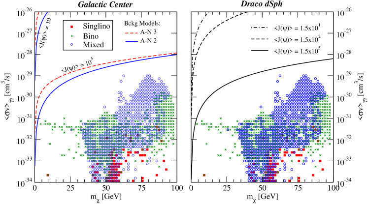
Figure 9: Prospects for the detection, with GLAST, of the monochromatic $\gamma\gamma$ gamma-ray line in the Galactic Center region (left) and in the Draco dSph (right). See the text for details. The conventions for the various neutralino types are as in Fig. 1.

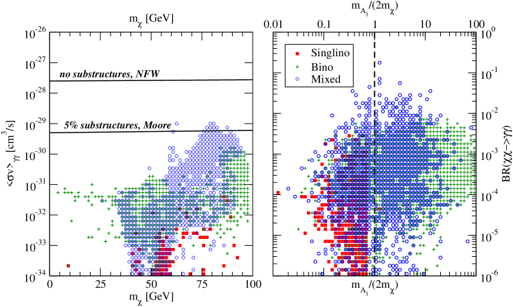
Figure 10: Prospects for the detection, with GLAST, of the monochromatic $\gamma\gamma$ gamma-ray line in the extra-galactic gamma-ray background. See the text for details. The conventions for the various neutralino types are as in Fig. 1.

In the formula above, we defined the dimensionless quantity

$$\overline{J}(\psi,\Delta\Omega)\equiv\frac{1}{\Delta\Omega}\int_{\Delta\Omega}{\rm d}\Omega\frac{1}{8.5\ {\rm kpc}}\left(\frac{1}{0.3\ {\rm GeV}/{\rm cm}^{3}}\right)^{2}\int_{\rm line\ of\ sight}\rho_{\rm DM}^{2}(l){\rm d}l(\psi).$$ (26)

We define a signal as “detectable” provided the number of signal events in the considered energy bin $N_{s}$ is larger than 5, and the following $5-\sigma$ significance condition is fulfilled:

$$\phi_{s}\sqrt{\frac{A_{\rm eff}\cdot T}{\phi_{b}+\phi_{s}}}>5.$$ (27)

Evaluating the gamma-ray background in the Galactic Center is certainly a non trivial task. Since the EGRET data from the Galactic Center likely include a gamma-ray source with a significant offset with respect to the actual Galactic Center Hooper:2002fx , we shall consider here the data from the HESS collaboration Aharonian:2004wa , which feature a much better angular resolution. The HESS data from the Galactic Center region indicate a steady power law gamma-ray source with a spectrum ${\rm d}N_{\gamma}/{\rm d}E\propto E_{\gamma}^{-2.2}$ extending over a range of gamma-ray energies of almost two orders of magnitude Aharonian:2004wa . The flux at low energies, $E_{\gamma}\simeq 200$ GeV, is limited by the experimental energy threshold. Extrapolating down to the energies of interest here (a few GeV up to 100 GeV) involves invoking a particular nature for the mechanism responsible for the gamma-ray production. Following Zaharijas:2006qb , we consider two extreme choices for the background extrapolation at lower energies, namely the models number 2 and 3 of Aharonian and Neronov, Ref. Aharonian:2004jr , (we shall indicate hereafter the two models as A-N2 and A-N3), respectively giving the smallest and the largest extrapolated background levels among those considered in Zaharijas:2006qb . Model A-N2 invokes inelastic proton-proton collisions of multi-TeV protons in the central super-massive black-hole accretion disk, while model A-N3 results from curvature and inverse Compton radiation. We assume $\phi_{0}\simeq 1\times 10^{-9}\ {\rm cm}^{2}{\rm s}^{-1}{\rm GeV}^{-1}$ and $\gamma=2.0$ for model A-N2, while $\phi_{0}\simeq 3\times 10^{-7}\ {\rm cm}^{2}{\rm s}^{-1}{\rm GeV}^{-1}$ and $\gamma=2.75$ for model A-N3.

As far as the values of $\overline{J}(0,\Delta\Omega)$ are concerned, we consider the range given by the extrapolation of the two halo models considered above (the Burkert and the adiabatically contracted N03 profiles), giving, roughly, $\overline{J}\simeq 10$ and $\overline{J}\simeq 10^{5}$. The left panel of Fig. 9 illustrates our results. All the sensitivity lines correspond to the criterion given in (27), which we find to be always more stringent than the $N_{s}>5$ requirement. The solid blue lines correspond to the A-N2 background model, while the A-N3 background is assumed for the red dashed lines. Our results show that even assuming a very optimistic dark matter profile, the likelihood of obtaining a significant gamma-ray line detection from the Galactic Center is rather low; at the best, a weak excess can be detected either with very low mass neutralinos, or with mixed neutralino-singlino models with a mass $m_{\chi}\sim 60\div 80$ GeV.

In the case of Draco, the estimated background is only given by the diffuse gamma-ray background, which we parameterize with $\phi_{0}\simeq 6.3\times 10^{-11}\ {\rm cm}^{2}{\rm s}^{-1}{\rm GeV}^{-1}$ and $\gamma=2.1$. We follow the results of Ref. Colafrancesco:2006he as far as the estimate of $\overline{J}$ are concerned; conservatively, a range of viable halo profiles for Draco gives $10\lesssim\overline{J}\lesssim 100$. Taking into account the possibility of a central super-massive black-hole and the subsequent adiabatic of dark matter in a central “spike” Colafrancesco:2006he can greatly enhance the viable values of $\overline{J}$, up to the level of $10^{5}$, a value we assume for the black solid line. As for the Galactic Center, the prospects of cleanly detecting a gamma-ray line from the direction of Draco do not seem particularly exciting, although, again, some models might in principle, and very optimistically, give some evidence of an energy-localized gamma-ray excess.

The monochromatic WIMP pair annihilation is also constrained by the contribution that annihilations occurring in any dark matter halo and at all redshifts give to the extragalactic gamma-ray radiation Bergstrom:2001jj ; Ullio:2002pj . We refer the reader to the thorough discussion given in Ref. Ullio:2002pj , and we make use here of the constraints, on the $m_{\chi},\langle\sigma v\rangle_{\gamma\gamma}$ plane derived in Fig. 15 of the same study. In particular, we report in Fig. 10, left, the sensitivity, on the above mentioned plane, expected from GLAST, under the two extreme scenarios for the halo profiles and the presence of dark matter substructures outlined in Ullio:2002pj . The upper curve refers to halos modeled by a NFW profile NFW , no substructures and concentration parameters inferred from the Bullock et al. model bullock , while the lower curve assumes the (cuspier) Moore et al. profile moore , with 5% of the halo mass in substructures with concentration parametes 4 times than that estimated with the Bullok et al. model. In the most generous scenario, a few mixed singlino-bino models can give rise to a detectable signal at GLAST, although more conservative assumptions leave small space for any hope of detecting any signature at all in the extra-galactic gamma-ray data.

Even though the prospects for the detection of the monochromatic line do not look particularly promising here, we wish to point out that the branching fractions we find, and the absolute values of $\langle\sigma v\rangle_{\gamma\gamma}$ are, typically, larger than in the MSSM. We devote App. A.2.1 to a detailed discussion of this point, but we wish here to emphasize the main reason why the NMSSM rate for the process $\chi\chi\rightarrow\gamma\gamma$ is expected to be more significant than in the MSSM. The potentially light extra CP-odd gauge boson gives rise to the extra contributions shown in Fig. 11; the size of this contribution, generically, depends upon whether the annihilation proceeds close to the $s$-channel resonance ($m_{\chi}\simeq m_{a_{1}}/2$). We illustrate the effect of the extra NMSSM diagrams in Fig. 10, right, where we show the size of ${\rm BR(\chi\chi\rightarrow\gamma\gamma)}$ as a function of the ratio $m_{a_{1}}/(2m_{\chi})$. As evident from the figure, the largest branching ratios occur when $m_{a_{1}}/(2m_{\chi})\sim 1$, and they are more than a couple of orders of magnitude larger than the MSSM limit (bino-like neutralinos and $m_{a_{1}}/(2m_{\chi})\gg 1$).

IV Conclusion

Gauge singlet extensions of the Higgs sector of the minimal supersymmetric Standard Model provide well motivated theoretical and phenomenological laboratories. Besides offering an elegant solution to the supersymmetric $\mu$ problem, they provide a viable way out of the difficulties connected to encompassing a mechanism of electroweak baryogenesis in the MSSM. In the present analysis, we focused on one specific such extension, the so-called NMSSM, and investigated, for the first time, the prospects for neutralino dark matter indirect detection.

The present study is motivated by two basic observations: first, in the NMSSM, unlike the MSSM, the lightest neutralino can be naturally very light, as a result of the possibility of it annihilating through a potentially very light extra CP-odd, mostly singlet-like Higgs boson; second, the extended Higgs sector leads to extra diagrams in the loop-amplitude relevant for the pair annihilation of neutralinos in photon or gluon pairs. An enhancement of the monochromatic $\chi\chi\rightarrow\gamma\gamma$ gamma-ray line is therefore generically expected within the NMSSM, as opposed to the minimal supersymmetric setup.

We found that the rate of neutrinos produced by the annihilation of neutralino dark matter particles captured inside the Earth and the Sun is in general large in the NMSSM; unlike the MSSM, we found that most models give a larger signal from annihilations in the core of the Earth rather than in the Sun, at a level which can, in certain cases, be constrained by current available data from SuperKamiokande and MACRO. This is presumably due in part to additional low velocity contributions to the local neutralino density in the region of the Earth which can result for light neutralinos. Future neutrino telescopes with increased sensitivity for low neutrino energies will be able to probe a sizable part of the parameter space by looking at signals from both the Earth and the Sun.

The dynamics of the Sun could also be modified due to energy transport by neutralinos. Our estimates show that, especially bino-like, neutralinos below $m_{\chi}\lesssim 30\ {\rm GeV}$ might contribute a significant fraction of the total solar luminosity. More detailed studies, using self-consistent solar models, could unveil large enough modifications on the sound speed or on the boron neutrino flux to significantly disfavor light neutralino scenarios.

We showed that within the NMSSM the expected antimatter yield from neutralino pair annihilations in the galactic halo can be sizable, although the absolute normalization of the flux depends on specific assumptions about the dark matter halo profile. In particular, we found that signals at low-energy antideuteron search experiments such as GAPS, and at space-based antimatter search experiments such as PAMELA, are expected, though not guaranteed, for very light neutralinos ($m_{\chi}\lesssim 20$ GeV) or for intermediate mass mixed singlino-bino neutralinos ($60\lesssim m_{\chi}\lesssim 90$ GeV).

We worked out for the first time the loop-induced pair annihilation cross section for NMSSM neutralinos into two photons and two gluons, pointing out that the expected branching ratio, with respect to tree-level neutralino pair annihilation into other Standard Model particles, is typically large, especially when compared to the MSSM case. The reason for this enhancement is traced back to diagrams which are resonant when $2m_{\chi}\simeq m_{a_{1}}$, the latter quantity indicating the mass of the lightest, extra CP-odd Higgs boson.

We analyzed in detail the prospects for the detection of the monochromatic gamma-ray line resulting from $\chi\chi\rightarrow\gamma\gamma$ annihilation processes in the Galactic Center, in a nearby dwarf spheroidal Galaxy (Draco) and the coherent effect of annihilations in any dark matter halo contributing to the extra-galactic gamma-ray radiation. We pointed out that most models are not expected to give any detectable signal at GLAST, although this detection channel looks significantly more promising than in the usual MSSM setup.

Finally, with the purpose of making the present study a useful and complete starting point for future research in the field, and in order to sort out and clarify some notational ambiguities and inconsistencies, we collect in the Appendix the details of the one-loop computation of the $\chi\chi\rightarrow\gamma\gamma,\ gg$ amplitudes and other quantities relevant for the estimate of indirect detection rates.

Appendix A Neutralino annihilation channels

A.1 Tree level processes

Analytic expressions for the NMSSM-like neutralino annihilation into two particles at tree level can be found in Stephan:1997ds .

For the study of indirect detection, only the nonzero terms in the limit $v\rightarrow 0$ need to be taken into account, which restricts the relevant processes to those with a CP-odd final state that have a non-vanishing $S$-wave amplitude.

With respect to the MSSM, the main differences are:

• An additional scalar Higgs, $h_{3}$, exchange in the $s$ channel contributes to the annihilation to $W^{+}W-$ and $ZZ$.

• A fifth neutralino is exchanged in the $t$ and $u$ channels for the $ZZ$ process.

• There is an extra $Z$ – scalar Higgs final state: $Zh_{3}$. Two Higgs pseudo-scalars instead of one, and five neutralinos contribute to these reactions.

• For the $W^{-}H^{+}$ final state, one has to take into account the contribution of the extra $h_{3}$ and $a_{2}$ Higgses.

• There are five additional final states with a scalar and a pseudoscalar Higgs. Diagrams $\widetilde{\chi_{5}^{0}}$ have to be considered.

• Finally, for the $f-\bar{f}$ final state, one has to include the exchange of the additional Higgses $h_{3}$ and $a_{2}$.

On top of that, the different couplings have contributions proportional to $\lambda$ and $\kappa$ not in the MSSM Ellwanger:2005dv . We used the $v$-independent part of the $S$-wave terms in Stephan:1997ds for our predictions in Section III.

A.2 One loop processes

A.2.1 Neutralino annihilation into two photons

Some radiative processes, even if loop suppressed, are of interest for dark matter detection. The annihilation to two photons, ${\widetilde{\chi}_{1}^{0}}{\widetilde{\chi}_{1}^{0}}\rightarrow\gamma\gamma$, has a characteristic monochromatic signature at $E_{\gamma}=m_{\widetilde{\chi}_{1}^{0}}/2$. This allows a clear distinction from all astrophysical backgrounds, unlike the continuum spectrum produced in tree level processes.

In the context of the MSSM, a full one-loop calculation was performed in Bergstrom:1997fh ; Bern:1997ng . We computed the cross-section for this process in the NMSSM by adapting the results of Bergstrom:1997fh .

Apart from the dependence on $\lambda$ and $\kappa$ of the NMSSM couplings, we need to compute two additional diagrams, shown in Fig. 11, due to the presence of a second pseudoscalar Higgs boson, $a_{2}$.

Figure 11: Additional diagrams, due to the second CP-odd Higgs boson, for the process ${\widetilde{\chi}_{1}^{0}}{\widetilde{\chi}_{1}^{0}}\rightarrow\gamma\gamma$ in the NMSSM. The contribution of $a_{1}$ corresponds to Fig. 1.d (left) and 2.d (right) in Bergstrom:1997fh for the MSSM.

Four types of Feynman diagrams, contributing to the two photon annihilation amplitude, were identified in Bergstrom:1997fh . Let us discuss their computation in the NMSSM in turn:

Diagrams 1.a-1.d

For the fermion–sfermion loop diagrams, we need to duplicate the CP-odd Higgs terms (Fig. 11) and substitute the NMSSM couplings in $S_{f\bar{f}}$, $D_{f\bar{f}}$, $G_{Zf}$ and $G_{a_{i}f}$ of Eqs. (7) and (8) in Bergstrom:1997fh .

For up-type quarks, let us define:

$$g_{ll} = \frac{-g_{2}m_{q}N_{13}}{\sqrt{2}m_{W}\sin\beta}$$

$$g_{rl} = \mp\frac{g_{2}N_{12}+(\pm 2e_{q}-1)g_{y}N_{11}/3}{\sqrt{2}}$$

$$g_{lr} = \sqrt{2}g_{y}N_{11}e_{q}$$

$$g_{rr} = g_{ll}$$ (28)

where $g_{2}$ is the electroweak coupling constant, $g_{y}=g_{2}\tan\theta_{W}$, $e_{q}$ is the quark charge and $m_{q}$ its mass. For down quarks and leptons we need to replace $N_{13}\rightarrow N_{14}$ and $\sin\beta\rightarrow\cos\beta$ and use the lower sign for $g_{rl}$. Then, with:

$$g_{1} = g_{ll}\cos\theta_{\widetilde{q}}+g_{lr}\sin\theta_{\widetilde{q}}$$

$$g_{2} = -g_{rl}\sin\theta_{\widetilde{q}}+g_{rr}\cos\theta_{\widetilde{q}}$$ (29)

where $\widetilde{q}$ is the squark mixing angle which is taken to be $\widetilde{q}=0$ (i.e. no mixing) for the first two families in Nmhdecay.

we have:

$$S_{f\bar{f}} = \frac{g_{1}^{2}+g_{2}^{2}}{2}$$

$$D_{f\bar{f}} = g_{1}g_{2}$$ (30)

The $Z{\widetilde{\chi}_{1}^{0}}{\widetilde{\chi}_{1}^{0}}$ coupling reads:

$$G_{Zf}=\frac{g_{2}^{2}T_{3f}}{\cos^{2}\theta_{w}}\left(N_{13}^{2}-N_{14}^{2}\right)$$ (31)

where the weak isospin, $T_{3f}$ is $+1/2$ for up-type quarks and $-1/2$ for down quarks and leptons.

Finally, using the $a_{i}{\widetilde{\chi}_{1}^{0}}{\widetilde{\chi}_{1}^{0}}$ coupling from Ellwanger:2005dv :

$$g_{a_{a}\widetilde{\chi}_{i}^{0}\widetilde{\chi}_{j}^{0}} = \frac{\lambda}{\sqrt{2}}(P_{a1}\Pi_{ij}^{45}+P_{a2}\Pi_{ij}^{35}+P_{a3}\Pi_{ij}^{34})-\sqrt{2}\kappa P_{a3}N_{i5}N_{j5}$$ (32)

$$+\frac{g_{y}}{2}(P_{a1}\Pi_{ij}^{13}-P_{a2}\Pi_{ij}^{14})-\frac{g_{2}}{2}(P_{a1}\Pi_{ij}^{23}-P_{a2}\Pi_{ij}^{24}),$$

where $\Pi_{ij}^{ab}=N_{ia}N_{jb}+N_{ib}N_{ja}$, we obtain:

$$G_{a_{i}f}=-2g_{a_{i}{\widetilde{\chi}_{1}^{0}}{\widetilde{\chi}_{1}^{0}}}\frac{m_{q}g_{2}P_{i1}}{m_{w}\sin\beta}$$ (33)

Changing $\sin\beta\rightarrow\cos\beta$ and $P_{i1}\rightarrow P_{i2}$ in Eq. (33), leads to the corresponding expression for down-type quarks and leptons.

Diagrams 2.a-2.d

For the chargino–Higgs loop diagrams need also to take into account the additional contribution of $a_{2}$ and use the expressions below for $S_{\chi H}$, $D_{\chi H}$, $G_{Z\chi}$ and $G_{a_{i}\chi}$ in Eq. (9) of Bergstrom:1997fh .

Taking the $H^{+}{\widetilde{\chi}_{1}^{0}}\chi^{-}$ coupling from Ellwanger:2005dv :

$$g_{H^{+}\chi^{-}_{i}\chi^{0}_{j}} = \lambda\cos\beta U_{i2}N_{j5}-\frac{\sin\beta}{\sqrt{2}}U_{i2}(g_{y}N_{j1}+g_{2}N_{j2})+g_{2}\sin\beta U_{i1}N_{j4}$$

$$g_{H^{-}\chi^{+}_{i}\chi^{0}_{j}} = \lambda\sin\beta V_{i2}N_{j5}+\frac{\cos\beta}{\sqrt{2}}V_{i2}(g_{y}N_{j1}+g_{2}N_{j2})+g_{2}\cos\beta V_{i1}N_{j3},$$ (34)

where $U$ and $V$ are the chargino mass matrices. we get:

$$S_{\chi H} = \frac{g_{H^{+}\chi^{-}_{i}{\widetilde{\chi}_{1}^{0}}}^{2}+g_{H^{-}\chi^{+}_{i}{\widetilde{\chi}_{1}^{0}}}^{2}}{2}$$

$$D_{\chi H} = g_{H^{+}\chi^{-}_{i}{\widetilde{\chi}_{1}^{0}}}g_{H^{-}\chi^{+}_{i}{\widetilde{\chi}_{1}^{0}}}.$$ (35)

The $Z$ exchange diagrams require:

$$G_{Z\chi}=\frac{g_{2}^{2}}{\cos^{2}\theta_{w}}\left(V_{i1}^{2}+\frac{V_{i2}^{2}}{2}-U_{i1}^{2}-\frac{U_{i2}^{2}}{2}\right)\left(N_{13}^{2}-N_{14}^{2}\right)$$ (36)

With Eq. (32) and the $a_{a}\chi^{+}_{i}\chi^{-}_{j}$ coupling:

$$g_{a_{a}\chi^{+}_{i}\chi^{-}_{j}}=\frac{\lambda}{\sqrt{2}}P_{a3}U_{i2}V_{j2}-\frac{g_{2}}{\sqrt{2}}(P_{a1}U_{i1}V_{j2}+P_{a2}U_{i2}V_{j1}),$$ (37)

we have:

$$G_{a_{i}\chi}=-4g_{a_{i}\chi^{+}_{j}\chi^{-}_{j}}g_{a_{i}{\widetilde{\chi}_{1}^{0}}{\widetilde{\chi}_{1}^{0}}}$$ (38)

Diagrams 3.a-3.c

The $W^{+}{\widetilde{\chi}_{1}^{0}}\chi^{-}_{j}$ couplings are:

$$g^{L}_{W1i} = g_{2}\left(-N_{13}V_{i2}/\sqrt{2}+N_{12}V_{i2}\right)$$

$$g^{R}_{W1i} = g_{2}\left(N_{14}U_{i2}/\sqrt{2}+N_{12}U_{i2}\right)$$ (39)

which we can substitute in $S_{\chi W}$ and $D_{\chi W}$ of Eqs. (11) and (12) in Bergstrom:1997fh to obtain the chargino-W loop contribution.

Diagrams 4.a-4.b

The unphysical Higgs boson is orthogonal to the charged Higgs and we can derive its required coupling to neutralinos and charginos by adapting those of the charged Higgs in Ellwanger:2005dv :

$$g_{G^{+}\chi^{-}_{i}\chi^{0}_{j}} = \lambda\sin\beta U_{i2}N_{j5}-\frac{\cos\beta}{\sqrt{2}}U_{i2}(g_{y}N_{j1}+g_{2}N_{j2})+g_{2}\cos\beta U_{i1}N_{j4}$$

$$g_{G^{-}\chi^{+}_{i}\chi^{0}_{j}} = \lambda\cos\beta V_{i2}N_{j5}+\frac{\sin\beta}{\sqrt{2}}V_{i2}(g_{y}N_{j1}+g_{2}N_{j2})+g_{2}\sin\beta V_{i1}N_{j3}.$$ (40)

Then, in Eq. (13) of Bergstrom:1997fh we need to input:

$$S_{\chi G} = \frac{g_{G^{+}\chi^{-}_{i}{\widetilde{\chi}_{1}^{0}}}^{2}+g_{G^{-}\chi^{+}_{i}{\widetilde{\chi}_{1}^{0}}}^{2}}{2}$$

$$D_{\chi G} = g_{G^{+}\chi^{-}_{i}{\widetilde{\chi}_{1}^{0}}}g_{G^{-}\chi^{+}_{i}{\widetilde{\chi}_{1}^{0}}}.$$ (41)

In the expressions above, we have not taken into account that Nmhdecay uses a real neutralino and chargino mass matrix, whereas the expressions in Bergstrom:1997fh assume that diagonalization in the neutralino and chargino sectors is performed using a complex $N$, $U$ and $V$, so that $m_{\widetilde{\chi}_{1}^{0}}$ and the chargino masses are always positive.

To correct for this fact we need to multiply by $\epsilon\equiv{\rm sign}\left(m_{\widetilde{\chi}_{1}^{0}}\right)$ all instances of $N^{*}$ in Bergstrom:1997fh for a vertex in which the neutralino is annihilated Gunion:1984yn and a similar change of sign needs to be done in $V$. Details for each vertex can be found, for the MSSM, in Edsjo:1997hp . For the two photon amplitude computation, this prescription amounts to multiplying by $\epsilon$ ($\eta\equiv{\rm sign}(m_{\widetilde{\chi}_{1}^{0}}m_{\chi^{+}})$) the $D$ terms in diagrams of type 1 (2, 3 and 4).

The presence of extra light CP-odd Higgses, can enhance the cross section for this process. In Fig. (12), we show the branching ratio for the process ${\widetilde{\chi}_{1}^{0}}{\widetilde{\chi}_{1}^{0}}\rightarrow\gamma\gamma$ together with the contribution from the diagrams in Fig. 11.

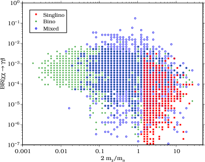
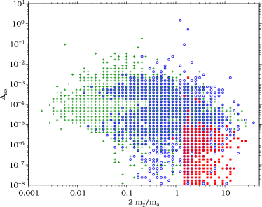
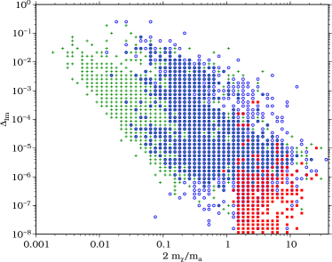
Figure 12: Branching ratio for the annihilation to $\gamma\gamma$ (up) and contribution of the CP-odd Higgs exchange diagrams to the real (left) and imaginary (right) part of the amplitude.

The branching ratio peaks for neutralino masses $2m_{\widetilde{\chi}_{1}^{0}}\sim m_{a_{1}}$, more so, for singlino and mixed-like neutralinos. The contribution of the CP-odd Higgs diagrams, Fig. 11, to the total Feynman amplitude, ${\cal A}$, is displayed in the lower panels by the quantity

$$\Delta=\frac{1}{\left|1-\frac{{\cal A}_{a_{i}}}{{\cal A}}\right|}.$$ (42)

Larger values of $\Delta$, corresponding to larger relative contributions of the CP-odd diagrams to the total amplitude, also cluster for those values where the branching ratio is larger.

The light CP-odd Higgses, together with the additional singlino component, lead, thus, to an enhancement of the $\gamma\gamma$ annihilation channel in the NMSSM compared to the MSSM.

A.2.2 Annihilation into two gluons

The cross section for this process Drees:1993bh can be obtained at once from the two photon channel computed in the previous section. In order to do so, we need to consider only the diagrams of type 1 for quarks, with no contribution from leptons. The electric charge is substituted by $e_{q}^{2}\rightarrow 1$, and the color sum average is performed by $\alpha_{em}^{2}\rightarrow 2\alpha_{s}^{2}$ in the final expression for $\sigma v$ Bergstrom:1997fh .

Appendix B Elastic scattering cross sections

We review here the computation of the neutralino-nucleon elastic cross-section, which is used to predict direct detection rates and, in the context of indirect detection, determines the capture rate of neutralinos in the Sun or in the Earth.

The basic ingredient for the neutralino-nucleon cross-section is the individual neutralino-quark cross-section, which for the MSSM can be found in Drees:1993bu . The $\chi-q$ process has been studied before in the context of the NMSSM. First in Bednyakov:1998is , where both spin-independent and spin-dependent contributions were computed. More recently the problem was revisited in Cerdeno:2004xw , were only the spin-independent part was considered and a mistake in Bednyakov:1998is was corrected. The authors in Gunion:2005rw approximated the spin-independent interaction by assuming that the $t$–channel exchange of CP-even Higgses dominates. For our predictions in Sec. III, we re-derived the ${\widetilde{\chi}_{1}^{0}}-q$ cross-section for the NMSSM by extending the MSSM calculation Drees:1993bu .

The low energy $\chi-q$ effective lagrangian can be written as:

$${\cal L}_{eff}=d_{q}\bar{\widetilde{\chi}}\gamma^{\mu}\gamma_{5}\widetilde{\chi}\bar{q}\gamma_{\mu}\gamma_{5}q+f_{q}\bar{\widetilde{\chi}}\widetilde{\chi}\bar{q}q$$ (43)

where only contributions that don’t vanish when $v\rightarrow 0$ have been written. The first term describes the spin-dependent contribution and the second one the spin-independent one.

As in the MSSM we have two types of diagrams contributing to the spin-dependent interaction in the NMSSM, $Z$ exchange and squark exchange. For the spin-independent one, CP-even Higgs exchange and squark exchange contribute to $f_{q}$.

Following Drees:1993bu , let us define:

$$X = -\sqrt{2}\left[g_{2}T_{3f}N_{12}-g_{y}\left(T_{3f}-e_{q}\right)N_{11}\right]$$

$$Y = \sqrt{2}g_{y}e_{q}N_{11}$$

$$Z_{up} = -\frac{g_{2}m_{q}N_{13}}{\sqrt{2}\sin\beta m_{w}}\quad\quad Z_{down}=-\frac{g_{2}m_{q}N_{14}}{\sqrt{2}\cos\beta m_{w}}.$$ (44)

Then the couplings involving the lightest squark can be written as:

$$a_{\widetilde{q}_{1}} = \frac{1}{2}\left[\cos\theta_{q}(X+Z)+\sin\theta_{q}(Y+Z)\right]$$

$$b_{\widetilde{q}_{1}} = \frac{1}{2}\left[\cos\theta_{q}(X-Z)+\sin\theta_{q}(Z-Y)\right],$$ (45)

and the corresponding equations for the heavier eigenstate, $j=2$, are found taking $\sin\theta_{q}\rightarrow\cos\theta_{q}$ and $\cos\theta_{q}\rightarrow-\sin\theta_{q}$.

With that, the spin-dependent ${\widetilde{\chi}_{1}^{0}}-q$ interaction is given by:

$$d_{q}=\frac{1}{4}\sum_{j=1}^{2}{\frac{a^{2}_{\widetilde{q}_{j}}+b^{2}_{\widetilde{q}_{j}}}{m^{2}_{\widetilde{q}_{j}}-\left(m_{\chi}+m_{q}\right)^{2}}}-\frac{g_{2}^{2}}{4m_{w}^{2}}T_{3q}\frac{1}{2}\left(N_{13}^{2}-N_{14}^{2}\right),$$ (46)

where the sum runs over the squark eigenstates and the last term describes the $Z$ exchange contribution.

As for the spin-independent interaction, we have:

$$f_{q}=-\frac{1}{4}\sum_{j=1}^{2}{\frac{a^{2}_{\widetilde{q}_{j}}-b^{2}_{\widetilde{q}_{j}}}{m^{2}_{\widetilde{q}_{j}}-\left(m_{\chi}+m_{q}\right)^{2}}}-m_{q}\sum_{j=1}^{3}{\frac{g_{2}g_{H_{j}{\widetilde{\chi}_{1}^{0}}{\widetilde{\chi}_{1}^{0}}}S_{j1}}{m_{H_{j}}^{2}m_{w}\sin\beta}}.$$ (47)

Note that in the NMSSM we have three CP-even Higgses, included in the last term. For down type quarks, we need to replace in Eq. (47), $S_{j1}\rightarrow S_{j2}$ and $\sin\beta\rightarrow\cos\beta$. Also, we need the coupling $q-\widetilde{q}-{\widetilde{\chi}_{1}^{0}}$:

$$g_{h_{a}\chi^{0}_{i}\chi^{0}_{j}} = \frac{\lambda}{\sqrt{2}}(S_{a1}\Pi_{ij}^{45}+S_{a2}\Pi_{ij}^{35}+S_{a3}\Pi_{ij}^{34})-\sqrt{2}\kappa S_{a3}N_{i5}N_{j5}$$ (48)

$$-\frac{g_{1}}{2}(S_{a1}\Pi_{ij}^{13}-S_{a2}\Pi_{ij}^{14})+\frac{g_{2}}{2}(S_{a1}\Pi_{ij}^{23}-S_{a2}\Pi_{ij}^{24}).$$

Our expression for the spin-dependent interaction agrees with the computation in Bednyakov:1998is . As for the spin-independent part, the authors in Cerdeno:2004xw noted a mistake in the expressions given in Bednyakov:1998is . We agree with their remark, but note that the $q-\widetilde{q}-{\widetilde{\chi}_{1}^{0}}$ couplings given in Cerdeno:2004xw contain a mistake, since the couplings for $\widetilde{q_{2}}$ cannot be obtained from those of $\widetilde{q_{1}}$ by the usual change $\sin\theta_{q}\rightarrow\cos\theta_{q}$ and $\cos\theta_{q}\rightarrow-\sin\theta_{q}$. Indeed, the sign in front of $N^{*}_{\alpha 2}$ should affect the whole coefficient of the $\sin\theta_{q}$ term in their Eq. (A.11).

Since we have used a real neutralino matrix $N_{ij}$, we should add the necessary factors of $\epsilon$ in the expressions above. We have followed Drees:1993bu , where a real $N_{ij}$ was used, and where it was pointed out that the absolute value should be used in the kinematic factors appearing in various denominators. However, following the prescription in Gunion:1984yn , one can check that when $m_{\widetilde{\chi}_{1}^{0}}<0$, one should also take $f_{q}\rightarrow\epsilon f_{q}$. This extra sign difference, however, does not affect the nucleon cross sections discussed below, for they depend quadratically on $f_{q}$ or $d_{q}$.

Once the individual ${\widetilde{\chi}_{1}^{0}}-q$ cross sections are determined, we can proceed to compute the nucleon (proton or neutron) cross sections used in Sec. III.

The spin-independent nucleon-neutralino elastic cross section is given by:

$$\sigma^{si}_{p,n}=\frac{4m_{r}^{2}}{\pi}f_{p,n}^{2}$$ (49)

where

$$f_{p,n}=\sum_{q=u,d,s}{f_{Tq}^{p,n}f_{q}\frac{m_{p,n}}{m_{q}}}+\frac{2}{27}\left(1-\sum_{q=u,d,s}{f_{Tq}^{p,n}}\right)\sum_{q=c,b,t}{f_{Tq}^{p,n}f_{q}\frac{m_{p,n}}{m_{q}}}$$ (50)

and for the quark composition of each nucleon, $f_{Tq}^{p,n}$, we use the central values found in Bertone:2004pz . In Eq. (49), the reduced mass is $m_{r}\equiv m_{p,n}m_{\chi}/\left(m_{p,n}+m_{\chi}\right)$.

For the axial-vector interactions we need the nucleon spin carried by each quark. We use, again, the central values from Bertone:2004pz to find:

$$\sigma^{sd}_{p,n}=\frac{4m_{r}^{2}}{\pi}3\left(f_{u}\Delta_{u}^{p,n}+f_{d}\Delta_{d}^{p,n}+f_{s}\Delta_{s}^{p,n}\right)^{2}.$$ (51)

In Sec. III.2, scalar cross sections with nuclei are used. Since the values at zero momentum transfer are good enough for the task at hand, we compute them as:

$$\sigma_{i}=\frac{4m_{r}^{2}}{\pi}\left[Zf_{p}+(A-Z)f_{n}\right]^{2},$$ (52)

where $Z$ and $A$ are the atomic and mass numbers of the nucleus.

References

- (1) M. Bastero-Gil, C. Hugonie, S. F. King, D. P. Roy and S. Vempati, Phys. Lett. B 489, 359 (2000); R. Dermisek and J. F. Gunion, Phys. Rev. Lett. 95, 041801 (2005).
- (2) S. Eidelman et al. [Particle Data Group], Phys. Lett. B 592, 1 (2004).
- (3) J. E. Kim and H. P. Nilles, Phys. Lett. B 138, 150 (1984).
- (4) J. R. Ellis, J. F. Gunion, H. E. Haber, L. Roszkowski and F. Zwirner, Phys. Rev. D 39, 844 (1989); H. P. Nilles, M. Srednicki and D. Wyler, Phys. Lett. B 120, 346 (1983); J. M. Frere, D. R. T. Jones and S. Raby, Nucl. Phys. B 222, 11 (1983); J. P. Derendinger and C. A. Savoy, Nucl. Phys. B 237, 307 (1984); M. Drees, Int. J. Mod. Phys. A 4, 3635 (1989); U. Ellwanger, M. Rausch de Traubenberg and C. A. Savoy, Phys. Lett. B 315, 331 (1993); P. N. Pandita, Phys. Lett. B 318, 338 (1993); T. Elliott, S. F. King and P. L. White, Phys. Rev. D 49, 2435 (1994); B. Ananthanarayan and P. N. Pandita, Phys. Lett. B 371, 245 (1996); B. Ananthanarayan and P. N. Pandita, Phys. Lett. B 353, 70 (1995); F. Franke and H. Fraas, Int. J. Mod. Phys. A 12, 479 (1997); B. Ananthanarayan and P. N. Pandita, Int. J. Mod. Phys. A 12, 2321 (1997); U. Ellwanger and C. Hugonie, Eur. Phys. J. C 5, 723 (1998).
- (5) A. D. Sakharov, Pisma Zh. Eksp. Teor. Fiz. 5, 32 (1967) [JETP Lett. 5, 24 (1967)]; M. Carena, M. Quiros and C. E. Wagner, Phys. Lett. B 380, 81 (1996); D. Delepine, J. M. Gerard, R. Gonzalez Felipe and J. Weyers, Phys. Lett. B 386, 183 (1996); J. M. Cline and G. D. Moore, Phys. Rev. Lett. 81, 3315 (1998).
- (6) M. Carena, M. Quiros and C. E. M. Wagner, Nucl. Phys. B 524, 3 (1998); M. Carena, M. Quiros, M. Seco and C. E. M. Wagner, Nucl. Phys. B 650, 24 (2003); J. M. Cline, M. Joyce and K. Kainulainen, Phys. Lett. B 417, 79 (1998) [Erratum-ibid. B 448, 321 (1998)]; S. J. Huber, P. John and M. G. Schmidt, Eur. Phys. J. C 20, 695 (2001); P. Huet and A. E. Nelson, Phys. Rev. D 53, 4578 (1996); M. Aoki, N. Oshimo and A. Sugamoto, Prog. Theor. Phys. 98, 1179 (1997); C. Lee, V. Cirigliano and M. J. Ramsey-Musolf, Phys. Rev. D 71, 075010 (2005); C. Balazs, M. Carena, A. Menon, D. E. Morrissey and C. E. M. Wagner, Phys. Rev. D 71, 075002 (2005); C. Balazs, M. Carena and C. E. M. Wagner, Phys. Rev. D 70, 015007 (2004); V. Cirigliano, S. Profumo and M. J. Ramsey-Musolf, JHEP 0607, 002 (2006).
- (7) M. Pietroni, Nucl. Phys. B 402, 27 (1993); A. T. Davies, C. D. Froggatt and R. G. Moorhouse, Phys. Lett. B 372, 88 (1996); S. J. Huber and M. G. Schmidt, Nucl. Phys. B 606, 183 (2001); M. Bastero-Gil, C. Hugonie, S. F. King, D. P. Roy and S. Vempati, Phys. Lett. B 489, 359 (2000); J. Kang, P. Langacker, T. j. Li and T. Liu, Phys. Rev. Lett. 94, 061801 (2005); D. Delepine, R. Gonzalez Felipe, S. Khalil and A. M. Teixeira, Phys. Rev. D 66, 115011 (2002); A. Menon, D. E. Morrissey and C. E. M. Wagner, Phys. Rev. D 70, 035005 (2004); C. Grojean, G. Servant and J. D. Wells, Phys. Rev. D 71, 036001 (2005); M. Carena, A. Megevand, M. Quiros and C. E. M. Wagner, Nucl. Phys. B 716, 319 (2005).
- (8) K. Funakubo, S. Tao and F. Toyoda, Prog. Theor. Phys. 114, 369 (2005).
- (9) S. A. Abel, S. Sarkar and P. L. White, Nucl. Phys. B 454, 663 (1995).
- (10) C. Panagiotakopoulos and K. Tamvakis, Phys. Lett. B 446, 224 (1999).
- (11) F. Franke, H. Fraas and A. Bartl, Phys. Lett. B 336, 415 (1994); F. Franke and H. Fraas, Phys. Lett. B 353, 234 (1995).
- (12) F. Franke and H. Fraas, Int. J. Mod. Phys. A 12, 479 (1997); U. Ellwanger and C. Hugonie, Eur. Phys. J. C 5, 723 (1998); U. Ellwanger, M. Rausch de Traubenberg and C. A. Savoy, Nucl. Phys. B 492, 21 (1997); U. Ellwanger and C. Hugonie, Eur. Phys. J. C 25, 297 (2002); V. Barger, P. Langacker, H. S. Lee and G. Shaughnessy, Phys. Rev. D 73, 115010 (2006); V. Barger, P. Langacker and G. Shaughnessy, arXiv:hep-ph/0609068.
- (13) U. Ellwanger and C. Hugonie, arXiv:hep-ph/0508022.
- (14) B. R. Greene and P. J. Miron, Phys. Lett. B 168, 226 (1986); R. Flores, K. A. Olive and D. Thomas, Phys. Lett. B 245, 509 (1990); K. A. Olive and D. Thomas, Nucl. Phys. B 355, 192 (1991).
- (15) S. A. Abel, S. Sarkar and I. B. Whittingham, Nucl. Phys. B 392, 83 (1993).
- (16) A. Stephan, Phys. Rev. D 58, 035011 (1998).
- (17) G. Belanger, F. Boudjema, A. Pukhov and A. Semenov, arXiv:hep-ph/0607059.
- (18) G. Belanger, F. Boudjema, C. Hugonie, A. Pukhov and A. Semenov, JCAP 0509, 001 (2005).
- (19) D. A. Demir, M. Frank and I. Turan, Phys. Rev. D 73, 115001 (2006) [arXiv:hep-ph/0604168].
- (20) V. A. Bednyakov and H. V. Klapdor-Kleingrothaus, Phys. Rev. D 59, 023514 (1999).
- (21) D. G. Cerdeno, C. Hugonie, D. E. Lopez-Fogliani, C. Munoz and A. M. Teixeira, JHEP 0412, 048 (2004).
- (22) J. F. Gunion, D. Hooper and B. McElrath, Phys. Rev. D 73, 015011 (2006).
- (23) L. M. Krauss, K. Freese, D. N. Spergel and W. H. Press Astrophys. J. 299, 1001 (1985).
- (24) L. M. Krauss, M. Srednicki and F. Wilczek, Phys. Rev. D 33, 2079 (1986). T. K. Gaisser, G. Steigman and S. Tilav, Phys. Rev. D 34, 2206 (1986).
- (25) D. N. Spergel et al., arXiv:astro-ph/0603449.
- (26) L. Bergstrom and P. Ullio, Nucl. Phys. B 504, 27 (1997).
- (27) J. F. Gunion and H. E. Haber, Nucl. Phys. B 272, 1 (1986) [Erratum-ibid. B 402, 567 (1993)].
- (28) G. Hiller, Phys. Rev. D 70, 034018 (2004).
- (29) F. Wilczek, Phys. Rev. Lett. 40, 279 (1978).
- (30) R. Balest et al. [CLEO Collaboration], Phys. Rev. D 51, 2053 (1995).
- (31) M. A. Sanchis-Lozano, Int. J. Mod. Phys. A 19, 2183 (2004); N. Brambilla et al., arXiv:hep-ph/0412158; M. A. Sanchis-Lozano, PoS HEP2005, 334 (2006).
- (32) F. Franke and S. Hesselbach, Phys. Lett. B 526, 370 (2002); S. Y. Choi, D. J. Miller and P. M. Zerwas, Nucl. Phys. B 711, 83 (2005).
- (33) Z. Chacko, M. A. Luty, A. E. Nelson and E. Ponton, JHEP 0001, 003 (2000).
- (34) G. Bertone, D. Hooper and J. Silk, Phys. Rept. 405, 279 (2005).
- (35) G. Jungman, M. Kamionkowski and K. Griest, Phys. Rept. 267, 195 (1996).
- (36) J. L. Feng, K. T. Matchev and F. Wilczek, Phys. Rev. D 63, 045024 (2001).
- (37) Y. B. Zeldovich, A. A. Klypin, M. Y. Khlopov and V. M. Chechetkin, Yad. Fiz. 31, 1286 (1980).
- (38) J. Silk, K. A. Olive and M. Srednicki, Phys. Rev. Lett. 55, 257 (1985).
- (39) K. Freese, Phys. Lett. B 167, 295 (1986).
- (40) S. Ritz and D. Seckel, Nucl. Phys. B 304, 877 (1988).
- (41) K. Griest and D. Seckel, Nucl. Phys. B 283, 681 (1987) [Erratum-ibid. B 296, 1034 (1988)].
- (42) A. Gould, Astrophys. J. 321, 560 (1987).
- (43) W. H. Press and D. N. Spergel, Astrophys. J. 296, 679 (1985).
- (44) A. Gould, Astrophys. J. 321, 571 (1987); A. Gould, Astrophys. J. 368, 610 (1991).
- (45) J. N. Bahcall, M. H. Pinsonneault and S. Basu, Astrophys. J. 555, 990 (2001).
- (46) N. Grevesse and A. J. Sauval, Space Sci. Rev. 85, 161 (1998).
- (47) T. Damour and L. M. Krauss, Phys. Rev. Lett. 81, 5726 (1998); T. Damour and L. M. Krauss, Phys. Rev. D 59, 063509 (1999).
- (48) L. Bergstrom, J. Edsjo and P. Gondolo, Phys. Rev. D 55, 1765 (1997); L. Bergstrom, J. Edsjo and P. Gondolo, Phys. Rev. D 58, 103519 (1998).
- (49) P. Gondolo, J. Edsjo, P. Ullio, L. Bergstrom, M. Schelke and E. A. Baltz, JCAP 0407, 008 (2004).
- (50) A. Bottino, N. Fornengo, G. Mignola and L. Moscoso, Astropart. Phys. 3, 65 (1995). V. D. Barger, F. Halzen, D. Hooper and C. Kao, Phys. Rev. D 65, 075022 (2002).
- (51) E. Roulet, Phys. Lett. B 356, 264 (1995).
- (52) M. Cirelli, N. Fornengo, T. Montaruli, I. Sokalski, A. Strumia and F. Vissani, Nucl. Phys. B 727, 99 (2005).
- (53) M. Ambrosio et al. [MACRO Collaboration], Phys. Rev. D 60, 082002 (1999).
- (54) S. Desai et al. [Super-Kamiokande Collaboration], Phys. Rev. D 70, 083523 (2004) [Erratum-ibid. D 70, 109901 (2004)].
- (55) J. A. Aguilar et al. [The ANTARES Collaboration], Eur. Phys. J. C 33, S971 (2004).
- (56) A. Achterberg et al. [IceCube Collaboration], arXiv:astro-ph/0604450.
- (57) L. M. Krauss, “Cold Dark Matter Candidates and the Solar Neutrino Problem”, Harvard Preprint 85/A008a (1985).
- (58) D. N. Spergel and W. H. Press, Astrophys. J. 294, 663 (1985).
- (59) J. Faulkner and R. L. Gilliland, Astrophys. J. 299, 994 (1985).
- (60) S. Degl’Innocenti, W. A. Dziembowski, G. Fiorentini and B. Ricci, Astropart. Phys. 7, 77 (1997).
- (61) G. Fiorentini and B. Ricci, Phys. Lett. B 526, 186 (2002); J. N. Bahcall and C. Pena-Garay, New J. Phys. 6, 63 (2004).
- (62) I. P. Lopes, J. Silk and S. H. Hansen, Mon. Not. Roy. Astron. Soc. 331, 361 (2002); I. P. Lopes, G. Bertone and J. Silk, Mon. Not. Roy. Astron. Soc. 337, 1179 (2002).
- (63) I. Lopes and J. Silk, Phys. Rev. Lett. 88, 151303 (2002).
- (64) A. Bottino, G. Fiorentini, N. Fornengo, B. Ricci, S. Scopel and F. L. Villante, Phys. Rev. D 66, 053005 (2002).
- (65) A. Gould and G. Raffelt, Astrophys. J. 352, 654 (1990).
- (66) M. Nauenberg, Phys. Rev. D 36, 1080 (1987).
- (67) A. Gould and G. Raffelt, Astrophys. J. 352, 669 (1990).
- (68) S. Profumo and P. Ullio, JCAP 0407, 006 (2004).
- (69) P. Ullio, proceedings of the Third International Conference on Frontier Science, Monteporzio Catone (RM), ed. by Frascati Physics Series.
- (70) J. Edsjo, M. Schelke and P. Ullio, arXiv:astro-ph/0405414.
- (71) S. Profumo and C. E. Yaguna, Phys. Rev. D 70, 095004 (2004).
- (72) A. El-Zant, I. Shlosman and Y. Hoffman, Astrophys. J. 560, 336 (2001).
- (73) A. Burkert, Astrophys. J. 447, L25 (1995).
- (74) P. Salucci and A. Burkert, Astrophys. J. 537, L9 (2000).
- (75) G.R. Blumental, S.M. Faber, R. Flores and J.R. Primack, Astrophys. J. 301, 27 (1986).
- (76) P. Ullio, H.S. Zhao and M. Kamionkowski, Phys. Rev. D 64, 043504 (2001).
- (77) J. F. Navarro et al., Mon. Not. Roy. Astron. Soc. 349, 1039 (2004).
- (78) B. Moore, et al.,Astrophys. J. Lett. 524, L19 (1999).
- (79) T. Sjöstrand, PYTHIA 5.7 and JETSET 7.4. Physics and Manual, CERN-TH.7112/93, arXiv:hep-ph/9508391 (revised version).
- (80) F. Donato, N. Fornengo and P. Salati, Phys. Rev. D62, 043003 (2000).
- (81) L. Bergstrom, J. Edsjo and P. Ullio, Astrophys. J. 526, 215 (1999).
- (82) L.J. Gleeson and W.I. Axford, Astrophys. J. 149, L115 (1967).
- (83) P. Picozza et al., arXiv:astro-ph/0608697.
- (84) K. Mori, C. J. Hailey, E. A. Baltz, W. W. Craig, M. Kamionkowski, W. T. Serber and P. Ullio, Astrophys. J. 566, 604 (2002).
- (85) C. J. Hailey et al., JCAP 0601, 007 (2006).
- (86) H. Baer and S. Profumo, JCAP 0512, 008 (2005).
- (87) D. Hooper and J. Silk, Phys. Rev. D 71, 083503 (2005).
- (88) Galprop numerical package, http://www.mpe.mpg.de/~aws/propagate.html
- (89) S. Orito et al., Phys. Rev. Lett. 84 (1078), 2000; Y. Asaoka et al., Phys. Rev. Lett. 88 051101, (2002); Boezio et al., Astrophys. J. 561 787, (2001).
- (90) C. Grimani et al., A&A 392, 287 (2002); DuVernois et al., Astrophys. J. 559, 296 (2001); Boezio et al., Astrophys. J. 532, 653 (2000).
- (91) N. W. Evans, F. Ferrer and S. Sarkar, Phys. Rev. D 69, 123501 (2004); N. Fornengo, L. Pieri and S. Scopel, Phys. Rev. D 70, 103529 (2004).
- (92) L. Pieri, E. Branchini and S. Hofmann, Phys. Rev. Lett. 95, 211301 (2005); S. Profumo, Phys. Rev. D 72, 103521 (2005).
- (93) G. Zaharijas and D. Hooper, Phys. Rev. D 73, 103501 (2006).
- (94) L. Bergstrom and D. Hooper, Phys. Rev. D 73, 063510 (2006); S. Profumo and M. Kamionkowski, JCAP 0603, 003 (2006).
- (95) S. Colafrancesco, S. Profumo and P. Ullio, arXiv:astro-ph/0607073.
- (96) S. Colafrancesco, S. Profumo and P. Ullio, Astron. & Astrophys, 455, 21 (2006).
- (97) See www-glast.slac.stanford.edu/software/IS/glast_lat_performance.htm.
- (98) D. Hooper and B. Dingus, Proceedings of the 34th COSPAR Scientific Assembly: The 2nd World Space Congress, Houston, Texas, 10-19 Oct 2002 [arXiv:astro-ph/0212509].
- (99) F. Aharonian et al. [The HESS Collaboration], Astron. Astrophys. 425, L13 (2004).
- (100) F. Aharonian and A. Neronov, “High energy gamma rays from the massive black hole in the galactic Astrophys. J. 619, 306 (2005).
- (101) L. Bergstrom, J. Edsjo and P. Ullio, Phys. Rev. Lett. 87, 251301 (2001).
- (102) P. Ullio, L. Bergstrom, J. Edsjo and C. G. Lacey, Phys. Rev. D 66, 123502 (2002).
- (103) J.F. Navarro, C.S. Frenk and S.D.M. White, Astrophys. J. 462, 563 (1996); Astrophys. J. 490, 493 (1997); V.R. Eke, J.F. Navarro and M. Steinmetz, Astrophys. J. 554, 114 (2001).
- (104) J.S. Bullock et al., Mon. Not. Roy. Astron. Soc. 321, 559 (2001).
- (105) Z. Bern, P. Gondolo and M. Perelstein, Phys. Lett. B 411, 86 (1997).
- (106) J. Edsjo, arXiv:hep-ph/9704384.
- (107) M. Drees, G. Jungman, M. Kamionkowski and M. M. Nojiri, Phys. Rev. D 49, 636 (1994).
- (108) M. Drees and M. Nojiri, Phys. Rev. D 48, 3483 (1993).