HIP-2006-42/TH

hep-ph/0609254

Thermodynamics of AdS/QCD

K. Kajantie^a , T. Tahkokallio^a,b , Jung-Tay Yee^b .

^aDepartment of Physics, P.O.Box 64, FIN-00014 University of Helsinki, Finland

^bHelsinki Institute of Physics, P.O.Box 64, FIN-00014 University of Helsinki, Finland

We study finite temperature properties of four dimensional QCD-like gauge theories in the gauge theory/gravity duality picture. The gravity dual contains two deformed 5d AdS metrics, with and without a black hole, and a dilaton. We study the thermodynamics of the 4d boundary theory and constrain the two metrics so that they correspond to a high and a low temperature phase separated by a first order phase transition. The equation of state has the standard form for the pressure of a strongly coupled fluid modified by a vacuum energy, a bag constant. We determine the parameters of the deformation by using QCD results for $T_{c}$ and the hadron spectrum. With these parameters, we show that the phase transition in the 4d boundary theory and the 5d bulk Hawking-Page transition agree. We probe the dynamics of the two phases by computing the quark-antiquark free energy in them and confirm that the transition corresponds to confinement-deconfinement transition.

1 Introduction

In the gauge-gravity duality picture the gravity dual of finite temperature ${\cal N}=4$ supersymmetric Yang-Mills theory is a 5-dimensional AdS space (times $S_{5}$) with a black hole [1, 2]. While this is a very special conformally invariant theory and requires also $g^{2}N_{c}\gg 1,N_{c}\gg 1$ for its validity, it has recently become apparent that one could meaningfully apply the gauge-gravity duality picture to QCD matter produced in relativistic heavy ion collisions, to viscosity [3, 4, 5], to jet energy loss [6, 7, 8, 9, 10, 11] and to photon production [12]. Note that these are all quasistatic phenomena; the gravity dual of a full dynamic heavy ion collision is unknown, for attempts, see [13, 14, 15].

Ideally, one would like to derive the gravity dual of QCD in a string theory framework, but this top-down way has so far not lead to a unique result. Instead, one has, in a phenomenological approach, studied various deformed metrics as candidate gravity duals of QCD-like theories [16, 17, 18, 19, 20, 21, 22, 23]. The purpose of this article is to continue this line and to present a gravity dual model for QCD thermodynamics. The model will cover both the deconfined phase (stable at $T>T_{c}$, metastable at $T<T_{c}$), the confined phase (stable at $T<T_{c}$, metastable at $T>T_{c}$) and the phase transition in between. The model for the high $T$ phase will be a deformed AdS black hole metric with a dilaton, the model for the low $T$ phase will be a deformed horizonless AdS metric with a dilaton. A deformation is defined as a multiplication of the 5d metric by an arbitrary function depending on the fifth coordinate $z$. The dilaton plays an essential role here. The phase transition will be analyzed in two independent ways: by computing the energy momentum tensor in the 4d boundary theory and by computing the difference of the 5d bulk actions [24, 2, 25, 26]. The shapes and parameters of the deformations of the two phases are fixed by using the QCD number for the $T_{c}$ of the 4d boundary theory and by using constraints from the $T=0$ hadron spectrum [23]. With these parameters the 5d bulk Hawking-Page transition coincides with the 4d boundary one. With the same parameters one can then also compute the $Q\bar{Q}$ free energy (see also [27, 28] in the two phases. The significant role of the dilaton is apparent here, the deformation in the string frame is qualitatively different from that in the Einstein frame. At $T=0$ we see that the $Q\bar{Q}$ potential contains a confining linear part but also string breaking, indicating that the deformation contains effects of dynamical quarks. At $T>T_{c}$ the $Q\bar{Q}$ pair becomes deconfined with entropy $\approx$ 2.1/pair.

The model we end up with is admittedly not unique and contains several parameters, but this is due to the fact that we wish to treat a large number of different QCD phenomena at the same time. Limiting oneself to one phenomenon at a time, simpler gravity duals can be presented. Our result shows that a comprehensive solution is possible.

The paper is organized as follows. In section 2, we specify the model. We assume a five dimensional gravity action with a dilaton and a matter Lagrangian and postulate two solutions corresponding to QCD-like theories on the boundary. In section 3, using gravity/gauge theory duality we compute the energy momentum tensor on the 4d boundary and find the phase structure of the boundary gauge theory. In section 4, we use the meson mass spectrum to constrain the parameters of our approach. In section 5, we consider a Hawking-Page type transition of the 5d bulk geometry and find the correspondence between the phase transition on the boundary and the phase transition in the bulk. In section 6, we compute the Wilson-Polyakov loops and correspondingly the free energy (potential at $T=0$) between a probe quark and antiquark. This confirms that, indeed, at high temperatures we are in the deconfined phase and at low temperature in the confined phase. Section 7 contains a discussion.

The numbers related to experimental ones quoted below should be understood to have a sizable ${\cal O}$(10%) error.

2 The Model

We consider the following five dimensional action in Einstein frame, in standard notation:

$$S={1\over 16\pi G_{5}}\int d^{5}x\sqrt{-g}\left(R-2\Lambda-{4\over 3}(\partial_{\mu}\Phi)^{2}\right)-{1\over 8\pi G_{5}}\oint d^{4}x\sqrt{-\gamma}\Theta+\int d^{5}x\sqrt{-g}e^{a\Phi}L_{m}.$$ (1)

The second term is the boundary term (for a boundary surface $z=\epsilon$) and the third term is the matter part, which we do not have to specify completely. The constant $a$ is dependent on the coupling of matter to gravity. This action can be the bosonic part of a supergravity action descendant from string theory. Note that even though we do not specify the origin of the model in detail, we have in mind near horizon geometry of stacked branes solution that gives asymptotically $AdS_{5}$ space. A nontrivial matter part can be introduced if we add, for example, a spacetime filling brane adding fundamental matter to the problem[29, 30, 31, 32]. The effect of the presence of fundamental matter would be already reflected in the full supergravity solution.

We assume that $L_{m}$ can be so chosen that the following metric is a solution as a dual to finite temperature QCD.

$$ds^{2}={\cal L}^{2}{e^{h(z)}\over z^{2}}\left[-g(z)dt^{2}+dx_{1}^{2}+dx_{2}^{2}+dx_{3}^{2}+{dz^{2}\over g(z)}\right],$$ (2)

with a dilaton $\Phi(z)$. The function $h(z^{2}),\,h(0)=0$ defines the deformation. The boundary theory lives at $z=0$ and the geometry would be asymptotically (when $z\to 0$) AdS. We shall define the string frame so that it contains the combination $\sqrt{-g}e^{-2\Phi}R$ in the action. The transformation between Einstein frame and string frame is then given by

$$g_{MN}^{(E)}=e^{-{4\over 3}\Phi}g_{MN}^{(s)}$$ (3)

and the bulk metric in the string frame will be the same as (2) but with

$$e^{h(z)}\Rightarrow e^{f(z)},\qquad f(z)\equiv h(z)+{4\over 3}\Phi(z).$$ (4)

Our gravity dual is defined by specifying the deformation $h(z)$ and the dilaton $\Phi(z)$. We will have two alternatives, one will be the stable phase for $T>T_{c}$, the other for $T<T_{c}$. The former is

$$h(z) = -cz^{2}$$

$$\Phi(z) = {3\over 4}\phi z^{2}$$

$$g(z) = 1-{z^{4}\over z_{0}^{4}},$$ (5)

and the latter

$$h(z) = -cz^{2}(1-{29\over 20}w(\sqrt{c}z))$$

$$\Phi(z) = {3\over 4}\phi z^{2}$$

$$g(z) = 1.$$ (6)

Here

$$z_{0}={1\over\pi T}$$ (7)

is the horizon radius of the metric (2), $c\approx 0.127$ GeV² is a constant determined from the $T_{c}$ of the QCD phase transition in the 4d boundary theory and $\phi\approx 0.311$ GeV² is a constant which, together with $w(\infty)\equiv w(x\to\infty)=-1.0$ is determined from the mass spectrum of QCD. A further property of the function $w(x)$ is that it for small $x$ should behave as $w(x)=x^{2}+{\cal O}(x^{4})$, also constrained by the QCD phase transition in the 4d boundary theory (to make the bag constant vanish in the low temperature phase). We can thus constrain the UV and IR limits of $w(x)$; the intermediate behavior affects details of the $Q\bar{Q}$ potential. We will use the ansätz

$$w(x)=2x^{2}e^{-x^{2}}-\tanh x^{2},$$ (8)

plotted in Fig.1. In the same figure we also show the combination $f(z)=29[w(\sqrt{c}z)-w(\infty)]cz^{2}/20$, later identified as the deformation of the low $T$ metric in the string frame Eq.(45). Further important constraints come from the fact that we want the phase transition in the 4d boundary theory and the Hawking-Page transition in the 5d bulk theory to agree. In particular, this is possible only if the metric deformations coincide for $z\to 0$, i.e., the constants $c$ and $\phi$ coincide in (2) and (2). The 5d bulk transition further constrains $c>0,\,w(\infty)<20/29$. Also note in the ansatz (2) and (2), we have assumed the dilaton and matter from $L_{m}$ have the same leading order behavior.

Figure 1: A plot of $w(z)$ defined by Eq.(8) (left) and a plot of the low $T$ metric string frame deformation $f(z)=29[w(\sqrt{c}z)-w(\infty)]cz^{2}/20$, $c=0.127$ GeV², $w(\infty)=-1$.

3 Thermodynamics of the Gauge Theory on the Boundary

We know that the metric (2) for $h=0$ is a solution of the 5d AdS equations

$$R_{MN}-{1\over 2}Rg_{MN}-{6\over{\cal L}^{2}}g_{MN}=0$$ (9)

and the boundary theory is hot ${\cal N}=4$ supersymmetric Yang-Mills theory in 4d at the temperature $T=1/\pi z_{0}$ with a pressure = 3/4 times the ideal gas value[33]. How is this affected by the introduction of the deformation $h(z)$? To be able to treat the two cases (2) and (2) simultaneously, write $h(z)=d_{1}z^{2}+d_{2}z^{4}+{\cal O}(z^{6})$, only the parameters $d_{1},d_{2}$ of dimension $T^{2},T^{4}$ matter for this problem.

To answer this question we should compute the energy-momentum tensor of the boundary theory. Since the theory is strongly coupled, the computation directly from the boundary field theory is not feasible, but we can use the gravity/gauge theory duality for this purpose. How this is to be done has been studied, say, in [34, 35, 36, 37, 38]. However, the general methods involve writing down an explicit 5d gravity-matter action and obtaining the metric and other matter fields as solutions of equations of motion. Here our starting point is a phenomenological deformed metric and the gravity action contains an unspecified matter Lagrangian. This unknown part will lead to an unknown part in the energy momentum tensor we obtain. It will cancel when studying the phase transition, computing the difference of pressures between two phases. Analoguously, in the later (Section 5) analysis of the phase transition as a bulk Hawking-Page transition in 5d, the unknown matter Lagrangian can be eliminated using equations of motion.

We transform the metric (2) to the form

$$ds^{2}=\frac{{\cal L}^{2}}{{\tilde{z}}^{2}}\big{(}g_{\mu\nu}(x,{\tilde{z}})dx^{\mu}dx^{\nu}+d{\tilde{z}}^{2}\big{)},$$ (10)

where $g_{\mu\nu}\to\eta_{\mu\nu}$ at ${\tilde{z}}=0$. If we expand the metric $g_{\mu\nu}$ for small ${\tilde{z}}$:

$$g_{\mu\nu}({\tilde{z}},x)=\eta_{\mu\nu}(x)+g^{(2)}_{\mu\nu}(x){\tilde{z}}^{2}+g^{(4)}_{\mu\nu}(x){\tilde{z}}^{4}+g^{(6)}_{\mu\nu}(x){\tilde{z}}^{6}+\ldots,$$ (11)

the energy-momentum tensor $T_{\mu\nu}$ of the boundary theory is given by [37]

$$T_{\mu\nu}(x)=\frac{{\cal L}^{3}}{4\pi G_{5}}[g^{(4)}_{\mu\nu}(x)+X_{\mu\nu}+Y_{\mu\nu}]={N_{c}^{2}\over 2\pi^{2}}[g^{(4)}_{\mu\nu}(x)+X_{\mu\nu}+Y_{\mu\nu}],$$ (12)

where

$$X_{\mu\nu} = -{1\over 8}\eta_{\mu\nu}[({\rm tr}\,g_{(2)})^{2}-{\rm tr}\,g_{(2)}^{2}]-{1\over 2}g_{(2){\mu\nu}}^{2}+{1\over 4}{\rm tr}\,g_{(2)}\cdot g_{(2){\mu\nu}}$$ (13)

$$= -C^{2}\eta_{\mu\nu}\quad{\rm if}\,\,g_{(2){\mu\nu}}=C\eta_{\mu\nu}$$

depends only on the square of contractions of $g_{(2)}$ and where

$$Y_{\mu\nu}=C_{m}\eta_{\mu\nu}$$ (14)

is a part depending on matter fields. We also used that for AdS${}_{5}\times S^{5}$ spacetime

$$G_{10}=G_{5}\pi^{3}{\cal L}^{5}={\pi^{4}{\cal L}^{8}\over 2N_{c}^{2}}.$$ (15)

For a thermal stationary and homogeneous system one, of course, has $g_{\mu\nu}({\tilde{z}},x)=g_{\mu\nu}({\tilde{z}})$.

Although we cannot determine the constant $C_{m}$ in (14), we expect it to be the same for both phases. This is analoguous to the fact that in our metric ansatz (2) and (2) the leading boundary behaviour of both the deformation $h(z)=-cz^{2}+\cdots$ and the dilaton $\Phi(z)={3\over 4}\phi z^{2}$ is the same in both metrics; which also imply that this holds for $g_{(2){\mu\nu}}$ computed below.

For the deformed metric (2) the transformation relating $z$ and ${\tilde{z}}$ is defined by

$$\int_{\epsilon}^{\tilde{z}}{d{\tilde{z}}\over{\tilde{z}}}=\int_{\epsilon}^{z}{e^{h(z^{2})/2}\over\sqrt{g(z)}}{dz\over z},$$ (16)

where we have enforced the condition ${\tilde{z}}\approx z$ for $z\to 0$ by putting the same $\epsilon$ as the lower limit in both integrations. This can be integrated to

$${\tilde{z}}^{2}={2z^{2}\over 1+\sqrt{g(z)}}\exp\biggl{[}\int_{0}^{z}dz{e^{h(z)/2}-1\over z\sqrt{g(z)}}\biggr{]},$$ (17)

For $h=0$, unmodified black hole, one can invert

$$z^{2}={{\tilde{z}}^{2}\over 1+{\tilde{z}}^{4}/(4z_{0}^{4})}$$ (18)

and get for the metric the exact result of [15]

$$ds^{2}={{\cal L}^{2}\over{\tilde{z}}^{2}}\left[-{(1-{\tilde{z}}^{4}/4z_{0}^{4})^{2}\over 1+{\tilde{z}}^{4}/4z_{0}^{4}}dt^{2}+(1+{{\tilde{z}}^{4}\over 4z_{0}^{4}})(dx_{1}^{2}+dx_{2}^{2}+dx_{3}^{2})+d{\tilde{z}}^{2}\right].$$ (19)

For any $h$, to invert (17) to express $z^{2}$ in terms of ${\tilde{z}}^{2}$, we expand in $z^{2}$ using the expanded form $h(z^{2})=d_{1}z^{2}+d_{2}z^{4}+...$, higher terms do not matter. One then obtains, for the high temperature metric (2) with the horizon $z_{0}$

$$g_{\mu\nu}=\eta_{\mu\nu}-{3\over 2}d_{1}\eta_{\mu\nu}{\tilde{z}}^{2}+[(u_{\mu}u_{\nu}+{1\over 4}\eta_{\mu\nu}){1\over z_{0}^{4}}-{20d_{2}-7d_{1}^{2}\over 16}\eta_{\mu\nu}]{\tilde{z}}^{4}+..,$$ (20)

where $u^{\mu}=(1,0,0,0)$ so that $u_{\mu}u_{\nu}+{1\over 4}\eta_{\mu\nu}={\rm diag}(3/4,1/4,1/4,1/4)$. Using (12),(13),(14) and (15) the energy-momentum tensor then is, for the high temperature metric,

$$T_{\mu\nu}=\left(\begin{array}[]{cccc}3aT^{4}+B_{h}&0&0&0\\ 0&aT^{4}-B_{h}&0&0\\ 0&0&aT^{4}-B_{h}&0\\ 0&0&0&aT^{4}-B_{h}\end{array}\right),$$ (21)

where

$$a={\pi^{2}N_{c}^{2}\over 8}\qquad B_{h}={N_{c}^{2}\over 32\pi^{2}}(-20d_{2}+29d_{1}^{2}-16C_{m})={N_{c}^{2}\over 32\pi^{2}}(29c^{2}-16C_{m}),$$ (22)

where we have inserted for the deformation of the high temperature metric (2) $d_{1}=c,\,d_{2}=0$. For the low temperature metric (2) there is no $T^{4}$ term,

$$T_{\mu\nu}=-B_{l}\eta_{\mu\nu}$$ (23)

with

$$B_{l}={N_{c}^{2}\over 32\pi^{2}}(-20d_{2}+29d_{1}^{2}-16C_{m})={N_{c}^{2}\over 32\pi^{2}}(-16C_{m}),$$ (24)

where we have constrained the low temperature metric deformation by $20d_{2}=29d_{1}^{2}$. The motivation for the omission of the $T^{4}$ term is that in the QCD phase transition there is a large change in the number of degrees of freedom when one crosses $T_{c}$. In fact, at large $N_{c}$, $p_{h}^{\prime}(T_{c})\sim{\cal O}(N_{c}^{2})$ while $p_{l}^{\prime}(T_{c})\sim{\cal O}(1)$ [39]. In the high $T$ phase there are gluons and quarks while the low $T$ phase only contains massless pions. The motivation for the constraint $20d_{2}=29d_{1}^{2}$ is that it minimises the vacuum energy in the low temperature phase in which the hadrons move in the true physical vacuum. For example, in the bag model for hot QCD matter one writes $p_{h}(T)=a_{h}T^{4}-B,\,\,p_{l}(T)=a_{l}T^{4}$ with $a_{h}\gg a_{l}$ .

Figure 2: The pressure $p(T)$ and entropy density $s(T)=p^{\prime}(T)$ in terms of temperature $T$ with $B=29c^{2}N_{c}^{2}/(32\pi^{2})$ and $L=T_{c}\Delta s=29N_{c}^{2}c^{2}/(8\pi^{2})$. The contribution of the matter fields is neglected here, $C_{m}\ll c^{2}$.

Thus our result for the pressures of the two phases is

$$p_{h}(T) = {\pi^{2}N_{c}^{2}\over 8}T^{4}-{N_{c}^{2}\over 32\pi^{2}}(29c^{2}-16C_{m})$$

$$p_{l}(T) = {N_{c}^{2}\over 32\pi^{2}}(16C_{m}),$$ (25)

and for the entropy density

$$s_{h}(T) = {\pi^{2}N_{c}^{2}\over 2}T^{3}$$

$$s_{l}(T) = 0,$$ (26)

The phase transition occurs at $p_{l}(T_{c})=p_{h}(T_{c})$. The unknown matter field contribution $C_{m}$ cancels from here, leading to

$$\pi T_{c}=\left({29\over 4}\right)^{1/4}\sqrt{c}.$$ (27)

This is what one dimensionally expects, introducing a deformation $\exp(cz^{2}+\cdots)$ one has, in addition to $T=1/\pi z_{0}$, introduced a new energy scale $c^{1/2}$ to the problem. Using (27) to determine the constant $c$ we have, e.g.,

$$T_{c}=186\,{\rm MeV}\Rightarrow c\approx 0.127\,{\rm GeV}^{2}.$$ (28)

The general behavior of the pressure $p(T)$ and entropy density $s(T)=p^{\prime}(T)$ is shown in Fig. 2. The transition corresponds to first order phase transition with two metastable branches persisting at all $T$. In section 6 we will show that the stable branch $T>T_{c}$ corresponds to a deconfined phase and that at $T<T_{c}$ to a confined phase.

For high temperature geometry (2), one can get the entropy directly from the geometrical data of the bulk, computing the area of black hole or evaluating the Euclidean action. If we calculate the entropy density from the area law, we get

$$s_{h}(T)={\pi^{2}N_{c}^{2}\over 2}T^{3}e^{-{3\over 2\pi^{2}}{c\over T^{2}}}.$$ (29)

This looks very interesting phenomenologically since it fits well with the lattice data[40] with proper adjustment of number of degrees of freedom. However, it differs from the result (3) for the entropy density. This is again due to the fact that we start from a deformed metric and do not derive it as a solution of 5d gravity-matter equations. For this complete treatment the results should concide [41] changing also the black hole entropy formula (29).

4 Meson Mass Spectrum

In this section, we show how it is possible within our framework to get a mass spectrum for mesons which grows linearly with the excitation level $n$ and spin $S$, i.e., $m^{2}\sim(n+S)$. We use the constraints, considered first in [23]: in the limit $z\to\infty$, the function $f(z)$ and the dilaton $\Phi(z)$ should behave as $f(z)\to z^{k}$, where $k<2$, and $\Phi(z)\to z^{2}$, to obtain a linear mass spectrum as a function of $n$ and $S$.

At zero temperature, we have the metric (2). We specify the matter part in (1) to contain a spin $S$ field :

$$S=\int d^{5}x\sqrt{-g}e^{-\Phi}\left({1\over 2}(DA_{S})^{2}+{1\over 2}M^{2}A_{S}^{2}\right),$$ (30)

where $A$ is totally symmetric rank $S$ tensor field. We are assuming that the matter in this case is open string matter on the spacetime filling branes, for example, and the coupling to the dilaton is fixed in this spirit. In the axial gauge, the equation of motion for the transverse traceless part, after rescaling $A_{S}=e^{(S-1)F(z)}\tilde{A}_{S}$ with $F(z)=f(z)-2\textrm{log}(z)$, is

$$\partial_{z}\left(e^{(S-{1\over 2})F}e^{-\Phi}\partial_{z}\tilde{A}_{S}\right)+m^{2}e^{(S-{1\over 2})F}e^{-\Phi}\tilde{A}_{S}=0.$$ (31)

After the substitution $\tilde{A}_{S}=e^{B\over 2}\psi$ with $B(z)=\Phi(z)-(S-{1\over 2})F(z)$, the equation is reduced to the Schrödinger form

$$\left(-\partial_{z}^{2}+V(z)\right)\psi=m^{2}\psi$$ (32)

with the potential

$$V(z)={1\over 4}(\partial_{z}B)^{2}-{1\over 2}\partial_{z}^{2}B.$$ (33)

To have the expected behavior of mass $m^{2}\sim n$, the asymptotic form of the potential should be quadratic [23]. This constrains the form of the metric strictly. We can read off of the asymptotical mass spectrum of spin $S$ meson from (2,2),

$$m^{2}=4\left[\frac{3}{4}\phi-(S-\frac{1}{2})\bigg{(}\phi-c(1-{29\over 20}w(\infty))\bigg{)}\right](n+S),$$ (34)

where $w(\infty)$ is the limiting value of the function $w(z)$ in (2) when $z\to\infty$. We have also used $\Phi(z)=\frac{3}{4}\phi z^{2}$. To match the experimental data [42], the term multiplying $S-1/2$ must be canceled. This fixes the value of the dilaton:

$$\phi=c\left(1-{29\over 20}w(\infty)\right).$$ (35)

For the $n$-excitations of the rho meson with spin $S=1$, $I^{G}J^{PC}=1^{+}1^{--}$ one obtains after this cancellation

$$m^{2}_{\rho}\simeq 3\phi\,n.$$ (36)

A linear fit to the observations is $m^{2}_{\rho}=0.93n$ GeV² [42]. Eq.(36) then gives $\phi=0.31$ GeV² and, using the earlier established value $c=0.127$ GeV², (35) gives $w(\infty)=-1.0$.

It is natural to expect that $g_{YM}^{2}\sim e^{\frac{3}{4}\phi z^{2}}$. In our case $\phi>0$, and the coupling flows toward strong coupling regime from UV to IR. Even though the direct comparison of the weakly coupled and strongly couple regime is impossible, this is still qualitatively consistent. In our notation, this also gives the condition that $w(\infty)<{20\over 29}$.

5 Hawking-Page Transition of the 5d Bulk Geometry

In section 3, we have computed the boundary energy momentum tensor for the deformed geometry which corresponds to finite temperature QCD on the boundary in terms of gravity/gauge theory duality. Notice again that the energy momentum tensor (21) is that of the 4d boundary theory and the phase transition is based on the 4d boundary theory picture. In this section we will try to compute the phase transition in the 5d bulk à la Hawking and Page [24]. First we Euclideanize the metric (2) performing the Wick rotation $t\rightarrow i\tau$, then evaluate the Euclidean action (1) corresponding to the two metrics (2) and (2). The metric corresponding to the smaller action is the stable one.

The action (1) contains the unspecified matter term $L_{m}$, but actually this can be eliminated using the equation of motion of the dilaton. The contribution to the action from the matter part is given by

$$S^{E}_{m}=-{1\over 6a\pi G_{5}}\int d^{5}x\partial_{z}[\sqrt{g}g^{zz}\partial_{z}\Phi]=-{1\over 6a\pi G_{5}}\int d\tau d^{3}x|_{z=\epsilon}^{z=z_{0},\infty}[\sqrt{g}g^{zz}\partial_{z}\Phi],$$ (37)

The upper limits $z=z_{0}$ and $z=\infty$ correspond to the metrics (2) and (2) and both give a vanishing contribution. The contribution from $z=\epsilon$ is divergent but the divergence is the same for the two metrics and thus cancels when the difference between the actions is evaluated. Thus the $L_{m}$-term can be entirely omitted from the discussion.

To evaluate the action for the remaining terms we have to specify the limits of integration in $\int d^{5}x=\int d\tau dzd^{3}x$. The integration over ${\bf x}$ is over all the space and thus gives only the volume factor $V_{3}$. The integration over $z$ is over $(\epsilon,z_{0})$ for (2) and over $(\epsilon,\infty)$ for (2). Since we are assuming that the black hole is in thermal equilibrium with thermal radiation, the high temperature geometry (2) has a natural temperature defined by the black hole temperature $\beta_{h}=\pi z_{0}$ and the integration over $\tau$ is over the interval $(0,\beta_{h})$. The temperature of thermal radiation in (2) can be arbitrary. For comparison with the high temperature metric, the temperature is fixed [24, 2] requiring that both have the same physical circumference along the Euclidean time direction $\tau$ at the regularization point $z=\epsilon$. This leads to the relation

$$\beta_{l}=\beta_{h}\sqrt{g_{h}/g_{l}}e^{(h_{h}-h_{l})/2}\big{|}_{z=\varepsilon}=\beta_{h}\sqrt{1-{\varepsilon^{4}\over z_{0}^{4}}}e^{-{29\over 40}c\varepsilon^{2}w(c\varepsilon^{2})}\simeq\beta_{h}\bigg{[}1-\bigg{(}\frac{1}{2z_{0}^{4}}+\frac{29c^{2}}{40}\bigg{)}\epsilon^{4}+\mathcal{O}(\epsilon^{6})\bigg{]}.$$ (38)

Since the $\tau$-integrals just give the upper limits, the action difference to be evaluated now is

$$\Delta S^{E} = S^{E}_{h}-S^{E}_{l}=-{V_{3}\beta_{h}\over 16\pi G_{5}}\left(\int_{\varepsilon}^{z_{0}}dz\,L_{h}-{\beta_{l}\over\beta_{h}}\int_{\varepsilon}^{\infty}dz\,L_{l}\right)+\Delta S_{\rm boundary},$$ (39)

where $L_{h}$ and $L_{l}$ are the Lagrangian densities without the $L_{m}$-term in (1) evaluated with the metrics (2) and (2), respectively. The $z$-integrals in (39) converge since $c>0$ and since the earlier result $w(\infty)=-1.0$ satisfies $w(\infty)<20/29$. The $\varepsilon\to 0$ divergences in (39) require a more careful analysis. The divergent parts of both of the Lagrangians are the same:

$$L_{div}=-\frac{8}{z^{5}}-\frac{16c}{z^{3}}+(27c^{2}-3\phi^{2})\frac{1}{z}.$$ (40)

but one also has to take into account the $\varepsilon^{4}$ term in $\beta_{l}/\beta_{h}$, Eq.(38). The result is:

$$\Delta S^{E}=-{V_{3}\beta_{h}\over 16\pi G_{5}}\bigg{(}\int_{0}^{z_{0}}dz(L_{h}-L_{l})-\int_{z_{0}}^{\infty}dzL_{l}-C\bigg{)},$$ (41)

where $C=-203c^{2}/20+1/z_{0}^{4}$ denotes the sum of the correction terms coming from the boundary term ($-58c^{2}/5$) and the temperature matching ($+29c^{2}/20+1/z_{0}^{4}$).

Computing numerically the difference of the actions for the metrics (2) and (2) and using the parameter values obtained earlier from the 4d boundary theory and the function $w(z)$ in (8), we obtain the result plotted in Fig. 3, in arbitrary units. The phase transition occurs when $\Delta S^{E}=0$ and this corresponds to $T_{c}\approx 0.181$ GeV. This is essentially the same as the $T_{c}=0.186$ GeV used to constrain the parameters of the 4d boundary theory. Exact agreement can be obtained by somewhat modifying the function $w(z)$ in (8), for example, by writing $w(z)=2z^{2}e^{-1.041z^{2}}-\tanh z^{2}$. Again we emphasize that we use the bulk computation to match the critical temperature obtained from the boundary computation instead of comparing the full thermodynamic functions to that of the boundary theory in every detail.

Figure 3: The difference $S^{E}_{h}-S^{E}_{l}$ between the actions computed with the metrics (2) and (2). The difference vanishes at $T\approx 0.181$ GeV, above that $S^{E}_{h}<S^{E}_{l}$ and the high $T$ metric (2) dominates.

6 $Q\bar{Q}$ Potential and Confinement-Deconfinement Transition

The $Q\bar{Q}$ potential (or free energy at finite $T$) in QCD can be “experimentally” measured using numerical lattice Monte Carlo techniques. Basically, one measures expectation values of rectangular Wilson-Polyakov loops with one of the sides becoming large. At finite $T$, the correlator of two Wilson-Polyakov lines $\langle{\rm Tr}\,W({\bf L}){\rm Tr}\,W({\bf 0})\rangle=\exp(-F(L,T)/T)$ measure the free energy at finite $T$.

To evaluate the $Q\bar{Q}$ potential we use standard gauge theory/gravity duality techniques (see, e.g., [45, 46]) to evaluate the finite $T$ expectation value of a Wilson-Polyakov loop of quarks of fundamental representation. Consider first a temporal-spatial loop. The Nambu-Goto action of a fundamental string then is

$$S_{\rm NG}={1\over 2\pi\alpha^{\prime}}\int d\tau d\sigma\sqrt{\det G_{MN}\partial_{a}X^{M}\partial_{b}X^{N}}.$$ (42)

Since we are interested in a temporal Wilson loop we choose the string coordinates as $X^{M}=(t,x,0,0,z)$, where $z=z(t,x)=z(x)$ is independent of time. The end points of the string are fixed at $z(0)=\pm L/2$ and $z(-x)=z(x)$. With the gauge choice of $\tau=t$ and $\sigma=x$ the string action becomes

$$S_{\rm NG} = {{\cal L}^{2}\over 2\pi\alpha^{\prime}}\Delta t\int_{-L/2}^{L/2}dx{e^{f(z)}\over z^{2}}\sqrt{z^{\prime}(x)^{2}+g(z)}$$ (43)

$$= {{\cal L}^{2}\over\pi\alpha^{\prime}}\Delta t\int_{\epsilon}^{z_{*}(L)}dz{e^{f(z)}\over z^{2}}\sqrt{1+g(z)x^{\prime}(z)^{2}},$$

where $z_{*}$ is the maximum value of $z$ (Fig4) and $\epsilon$ is a parameter used to regulate the UV divergence at $z=0$. A potential will be defined by $S_{\mbox{\scriptsize NG}}=V(L)\Delta t$.

The string frame deformation $f(z)$ is given in terms of the Einstein frame deformation $h(z)$ by Eq.(4), $f(z)=h(z)+4\Phi(z)/3$. Using Eqs. (2), (2) and (35) we have

$$f(z) = (\phi-c)z^{2}={29\over 20}[-w(\infty)]cz^{2}\quad{\rm high}\,T\,{\rm metric},$$ (44)

$$= {29\over 20}[w(\sqrt{c}z)-w(\infty)]cz^{2}\quad\quad\quad{\rm low}\,T\,{\rm metric},$$ (45)

where we earlier fixed $w(\infty)=-1$ and $c=0.127$ GeV². Due to the rapidly growing dilaton term the string frame deformation thus behaves qualitatively differently from the Einstein frame one: it grows monotonically $\sim+z^{2}$ for the high $T$ metric and is always $>0$ for the low $T$ metric.

The equation of motion following from (43) is simple and its first integral is

$${e^{f(z)}\over z^{2}}{g(z)\over\sqrt{z^{\prime}(x)^{2}+g(z)}}={\rm constant}={e^{f(z_{*})}\over z_{*}^{2}}\sqrt{g(z_{*})},$$ (46)

where the constant is given as the value of the left hand side when $z^{\prime}(x)=0$. From the symmetry of the problem this is at $x=0$, i.e., $z_{*}$ is the maximum value of $z$. Basically the solution can be of the three types as in Fig. 4.

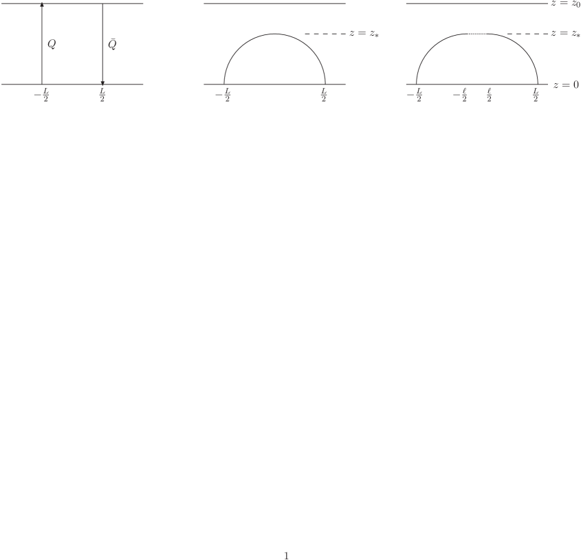
Figure 4: Three types of solutions: a $Q\bar{Q}$ solution (left), a solution with $z^{\prime}=0$ only at $z=z_{*}$ (middle), a solution with a constant piece at $z=z_{*}$ (right).

At high temperature with the metric (2), the equation of motion (46) has the following types of solutions (Fig4):

• A quark-antiquark solution (Fig.4 left)

  $$x=\pm L/2,\quad x^{\prime}(z)=0,\quad z^{\prime}(x)=\infty,\quad z_{*}=z_{0},$$ (47)

  with the action and the corresponding potential, regulated as discussed below,

  $$V_{Q\bar{Q}} = {{\cal L}^{2}\over\pi\alpha^{\prime}}\int_{\epsilon}^{z_{0}}dz{e^{f(z)}\over z^{2}}$$ (48)

  $$= {{\cal L}^{2}\over\pi\alpha^{\prime}}\left[{1\over\epsilon}+\int_{\epsilon}^{z_{0}}dz{1\over z^{2}}\left(e^{f(z)}-1\right)-{1\over z_{0}}\right]$$

  $$\Rightarrow {{\cal L}^{2}\over\pi\alpha^{\prime}}\left[\int_{0}^{z_{0}}dz{1\over z^{2}}\left(e^{f(z)}-1\right)-{1\over z_{0}}\right].$$ (49)

• A solution connecting the quark and antiquark with $z^{\prime}(x)=0$ only at $x=0$ (Fig.4 middle). Integration of (46) relates $z_{*}$ and $L$:

  $$L=2\int_{0}^{z_{*}}dz{1\over\sqrt{g(z)\left[q(z_{*})/q(z)-1\right]}},$$ (50)

  where

  $$q(z)=e^{-2f(z)}{z^{4}\over z_{0}^{4}-z^{4}},$$ (51)

  for high temperature phase and

  $$q(z)=e^{-2f(z)}z^{4},$$ (52)

  for low temperature phase. The corresponding potential is, regulating the $z\to 0$ divergence as discussed below,

  $$V(L,z_{0};f) = {{\cal L}^{2}\over\pi\alpha^{\prime}}\int_{\epsilon}^{z_{*}}{dz\over z^{2}}\,e^{f(z)}{1\over\sqrt{1-q(z)/q(z_{*})}}$$ (53)

  $$= {{\cal L}^{2}\over\pi\alpha^{\prime}}\left[{1\over\epsilon}+\int_{\epsilon}^{z_{*}}{dz\over z^{2}}\left(e^{f(z)}{1\over\sqrt{1-q(z)/q(z_{*})}}-1\right)-{1\over z_{*}}\right]$$

  $$\Rightarrow {{\cal L}^{2}\over\pi\alpha^{\prime}}\left[\int_{0}^{z_{*}}{dz\over z^{2}}\left(e^{f(z)}{1\over\sqrt{1-q(z)/q(z_{*})}}-1\right)-{1\over z_{*}}\right]$$ (54)

• One solution of the equation of motion also is (Fig.4 right)

  $$z=z_{*}={\rm constant}.$$ (55)

  This can be made a solution of required type by connecting its end points to the points $x(0)=\pm L/2$ by a solution of the previous type with nonzero $z^{\prime}(x)$. If the length of the constant piece is $\ell$, the value of $z_{*}$ will then be determined by (50) with $L\rightarrow L-\ell$ and the total potential is (54) evaluated for this $z_{*}(L-\ell)$ added to

  $$V_{\mbox{\scriptsize planar}}={{\cal L}^{2}\over 2\pi\alpha^{\prime}}{e^{f(z_{*})}\over z_{*}^{2}}\sqrt{g(z_{*})}\,\,\ell.$$ (56)

  For fixed $L=\ell+(L-\ell)$, $0\leq\ell<L$, we thus obtain a family of solutions with increasing length $\ell$ of the constant region, decreasing lengths $(L-\ell)/2$ of the two connecting regions at the ends and decreasing height $z_{*}$. It appears that at fixed $L$ all these solutions have a larger $V$ than the one of the middle type.

Figure 5: The functions $q(z)$ in Eq.(51) and $L(z_{*})$ in Eq.(50) for the high temperature metric with $T=400{\rm MeV}$ using the deformation (44) (upper two panels). The lower two panels show the same for the low temperature metric with $T=0$, now plotted vs $z$ in units of 1/GeV.

.

Eqs. (49) and (54) diverge for $z\to 0$ and have to be renormalized. There are two possibilities:

• Neglect the $1/\epsilon$ terms in (49) and (54) and put $\epsilon=0$ in the remainder;

• Subtract the two and put $\epsilon=0$ in the remainder, i.e., redefine $V$ as $V-V_{Q\bar{Q}}$.

We use the first one and the final potential is given by combining Eqs. (50), (49) and (54) so that the equilibrium state always corresponds to the smaller one of $V$ and $V_{Q\bar{Q}}$.

Figure 6: $V(L)$ vs $L$ as computed from eq. (54) for the low temperature metric (left, $T$-independent) and $F(L,T)$ vs $L$for the high temperature metric (right) at $T=500,300,T_{c}=186,100$ MeV. Note the difference in $L$-scales. The almost horizontal part of the low $T$ potential comes from the $z_{*}>6$ part of the $L(z_{*})$-curve in Fig.5, the horizontal parts of the high $T$ potential are $L$-independent values of $V_{Q\bar{Q}}$ from (49).

Consider first the low $T$ metric, using the deformation (45) and parameters obtained earlier. We plot $q(z)$ and $L(z_{*})$ with $z$ and $z_{*}$ in units of 1/GeV in Fig. 5. The structure in $L$ at small $z_{*}$ is significant and leads to up to three values of $V$ corresponding to one $L$ as seen in the plot of the ($T$-independent) potential $V(L)$ vs $L$ in Fig. 6. Tracing through the curve $L=L(z_{*})$ in Fig. 5 one can trace through the curve $V=V(L)$ in Fig. 6. The almost constant branch of $V(L)$ arises from the $z_{*}>6{\rm GeV}^{-1}$ part of $L(z_{*})$.

We interpret the resulting $T=0$ potential as showing a confining part for $L<1.2$ fm and a constant part for $L>1.2$ fm.

For $L<1.2\,\,{\rm fm}$ we can express the potential in Cornell form

$$V(L)=-{4\over 3}{\alpha_{s}\over L}+\sigma L.$$ (57)

If we use $\alpha_{s}\approx 0.36$, then we get the AdS radius ${\cal L}^{2}/(\pi\alpha^{\prime})\approx 0.67$ and $\sigma\approx 0.168{\rm GeV}^{2}$ or $\sqrt{\sigma}\approx 410{\rm MeV}$. This is in reasonable agreement with recent lattice data giving $\sqrt{\sigma}\approx 460$ MeV[43]. Note that $T_{c}/\sqrt{\sigma}\approx 0.46$ in this case.

Beyond 1.2 fm the potential is approximately constant and grows slowly from $\approx$ 0.9 GeV to $V_{Q\bar{Q}}=0.961$ GeV, obtained by evaluating Eq.(49) with $z_{0}=\infty$. One can speculate that the constant potential is an indication of QCD string breaking of dynamical quarks[47]. The constant part starts at 1.2 fm and its energy scale is about $1$ GeV. This should be in principle the twice the mass of the lightest hadron. Current lattice data indicates that the string breaking occurs about $1.2-1.4{\rm fm}$ at the energy scale of $1.0-1.2$ GeV [48]. This is consistent with our model calculation. The reason why we see the string breaking is not obvious at first thought because it happens only when dynamical quarks are included. However, from the consideration of linear Regge behavior of meson mass spectrum and the boundary thermodynamics we have been lead to a specific form of the function $w(z)$ containing a scale related to the mass scale of the fundamental matter in QCD. Thus in our model (2) we are already implicitly including dynamical quarks from the beginning. In AdS/CFT, light dynamical quarks can be added by introducing a spacetime-filling D7 brane [29]. It would be very interesting to see in supergravity whether the original metric ansätz (2) can be related to this flavor brane background.

Now that we have determined the AdS radius ${\cal L}^{2}/(\pi\alpha^{\prime})\approx 0.67$, we can draw the $Q\bar{Q}$ potential at high temperatures, again using the deformation (44) and parameters determined earlier. The quantities $q(z)$ and $L(z_{*})$ with $z$ and $z_{*}$ in units of $z_{0}$ are plotted in Fig. 5 and $V(L)$ in Fig. 6 for $T=400$ MeV. It is again useful to trace through $L(z_{*})$ and see how it maps to $V(L)$: one starts from $L=0,\,V=-\infty$, then $L$ and $V$ grow to a maximum value after which both again decrease but so that $V$ is almost constant. Finally again $L=0$ at $z_{*}=z_{0}$ at which point $V(L=0)=V_{Q\bar{Q}}$. This is $L$-independent and is shown as the horizontal curves in Fig.6.

One can observe the following for the high temperature phase:

• The overall potential is the lowest of the curves/line and contains the usual conformally invariant $V\sim-1/L$ at small $L$. At some $L$ this reaches $V_{Q\bar{Q}}$ and from this $L$ onwards the preferred state is the $Q\bar{Q}$ state with a constant $L$-independent potential. This is the structure observed already in [45] for an undeformed metric.

• At very large $T$, small $z_{0}$, the large $L$ value of the potential (free energy) $V_{Q\bar{Q}}$ from Eq.(49) approaches ${\cal L}^{2}/(\pi\alpha^{\prime})(-\pi T)$. Although one cannot strictly separate internal energy $E$ and entropy $S$ in the free energy of the $Q\bar{Q}$ state, this is compatible with $E=0,S={\cal L}^{2}/(\pi\alpha^{\prime})\cdot\pi\approx 2.1$. Notice that $\Delta S\sim{\cal O}(1)$ for simple quark and antiquark system.

• As the temperature decreases below $T_{c}$, a first order phase transition occurs as we have seen in sections 3 and 5. One can continue plotting $V(L)$ in this metastable phase, as done in Fig.6, and obtain a linear confining potential. However, the stable phase is the one corresponding to the metric (2) which should be used for $T<T_{c}$.

7 Discussion

In this paper, we have considered a 5d gravity action which presumably could descend from a higher dimensional fundamental theory. Following [23], we proposed a solution of the equations of motion that is dual to a QCD-like gauge theory on the 4d boundary. Using standard gravity/gauge theory duality correspondence we computed the 4d boundary energy-momentum tensor. The gauge dynamics on the boundary is that of a strongly coupled fluid modified by a vacuum energy. The bulk geometry was further constrained so that the 4d boundary theory shows a first order phase transition. With constraints from the hadron spectrum, the parameters of the deformation were fixed. Then we considered the 5d bulk transition following the recipe of Hawking and Page [24] and found that the geometric transition in the 5d bulk precisely matched with the phase transition on the 4d boundary. This is a remarkable correspondence and shows the power of gravity/gauge theory duality and the reasonableness of the model we have set up for the dual construction of QCD-like theories. The computation of quark-antiquark free energy (potential at $T=0$) showed that at $T=0$ potential contains a confining linear part but also string breaking, indicating that the deformation contains effects of dynamical quarks. At $T>T_{c}$ we saw a deconfined state with entropy = 2.1/pair.

In general terms, the whole setup started from three unknown functions, the deformations of the high $T$ and low $T$ metrics and the dilaton. We chose simple ansätze for the high $T$ deformation, $h(z)=-cz^{2}$, and for the dilaton, $\Phi(z)=\phi z^{2}$. The low $T$ deformation was then constrained in various ways and one ended up with the function $w(z)$ plotted in Fig.1. There is some freedom to change this function in the intermediate $z$ range, but not much without destroying the coincidence of the 4d boundary and 5d bulk transitions.

Many QCD-like features treated in this paper are basically IR dominant phenomena, but since from gravity/gauge theory duality, the boundary data is critically dependent on the boundary behavior of the bulk metric, the metric form in the UV region near the boundary becomes as important. If we solve the equations of motion of supergravity in top-down approach, this UV/IR behavior is naturally encoded in the solution, but when we approach phenomenologically we have to put this UV/IR behavior by hand. What we saw here is that the form of the metric is stringently constrained by this.

There are several directions of future study. First is to check the our ansätz using various physical quantities in QCD and refine the form of $w(z)$. Also it would be highly desirable to reproduce the solution in supergravity. Even though this is very difficult task, we have some better guiding principle at least.

Acknowledgement

We thank Esko Keski-Vakkuri, Mikko Laine and Kari Rummukainen for helpful discussions and Kostas Skenderis for valuable comments. This research has been supported by Academy of Finland, contract number 109720.

References

- [1] J. M. Maldacena, “The large N limit of superconformal field theories and supergravity,” Adv. Theor. Math. Phys. 2, 231 (1998) [Int. J. Theor. Phys. 38, 1113 (1999)] [arXiv:hep-th/9711200].
- [2] E. Witten, “Anti-de Sitter space, thermal phase transition, and confinement in gauge theories,” Adv. Theor. Math. Phys. 2, 505 (1998) [arXiv:hep-th/9803131].
- [3] G. Policastro, D. T. Son and A. O. Starinets, “The shear viscosity of strongly coupled N = 4 supersymmetric Yang-Mills plasma,” Phys. Rev. Lett. 87, 081601 (2001) [arXiv:hep-th/0104066].
- [4] P. Kovtun, D. T. Son and A. O. Starinets, “Viscosity in strongly interacting quantum field theories from black hole physics,” Phys. Rev. Lett. 94, 111601 (2005) [arXiv:hep-th/0405231].
- [5] P. Kovtun and A. Starinets, “Thermal spectral functions of strongly coupled N = 4 supersymmetric Yang-Mills theory,” Phys. Rev. Lett. 96, 131601 (2006) [arXiv:hep-th/0602059].
- [6] H. Liu, K. Rajagopal and U. A. Wiedemann, “Calculating the jet quenching parameter from AdS/CFT,” arXiv:hep-ph/0605178.
- [7] C. P. Herzog, A. Karch, P. Kovtun, C. Kozcaz and L. G. Yaffe, “Energy loss of a heavy quark moving through N = 4 supersymmetric Yang-Mills plasma,” JHEP 0607, 013 (2006) [arXiv:hep-th/0605158].
- [8] C. P. Herzog, “Energy loss of heavy quarks from asymptotically AdS geometries,” arXiv:hep-th/0605191.
- [9] A. Buchel, “On jet quenching parameters in strongly coupled non-conformal gauge theories,” arXiv:hep-th/0605178.
- [10] S. S. Gubser, “Drag force in AdS/CFT,” arXiv:hep-th/0605182.
- [11] E. Nakano, S. Teraguchi and W. Y. Wen, “Drag force, jet quenching, and AdS/QCD,” arXiv:hep-ph/0608274.
- [12] S. Caron-Huot, P. Kovtun, G. D. Moore, A. Starinets and L. G. Yaffe, “Photon and dilepton production in supersymmetric Yang-Mills plasma,” arXiv:hep-th/0607237.
- [13] H. Nastase, “The RHIC fireball as a dual black hole,” arXiv:hep-th/0501068.
- [14] E. Shuryak, S. J. Sin and I. Zahed, “A gravity dual of RHIC collisions,” arXiv:hep-th/0511199.
- [15] R. A. Janik and R. Peschanski, “Asymptotic perfect fluid dynamics as a consequence of AdS/CFT,” Phys. Rev. D 73, 045013 (2006) [arXiv:hep-th/0512162].
- [16] G. F. de Teramond and S. J. Brodsky, “The hadronic spectrum of a holographic dual of QCD,” Phys. Rev. Lett. 94, 201601 (2005) [arXiv:hep-th/0501022].
- [17] J. Erlich, E. Katz, D. T. Son and M. A. Stephanov, “QCD and a holographic model of hadrons,” Phys. Rev. Lett. 95, 261602 (2005) [arXiv:hep-ph/0501128].
- [18] L. Da Rold and A. Pomarol, “Chiral symmetry breaking from five dimensional spaces,” Nucl. Phys. B 721, 79 (2005) [arXiv:hep-ph/0501218].
- [19] F. Bigazzi, R. Casero, A. L. Cotrone, E. Kiritsis and A. Paredes, JHEP 0510, 012 (2005) [arXiv:hep-th/0505140].
- [20] L. Da Rold and A. Pomarol, “The scalar and pseudoscalar sector in a five-dimensional approach to JHEP 0601, 157 (2006) [arXiv:hep-ph/0510268].
- [21] K. Ghoroku, N. Maru, M. Tachibana and M. Yahiro, “Holographic model for hadrons in deformed AdS(5) background,” Phys. Lett. B 633, 602 (2006) [arXiv:hep-ph/0510334].
- [22] E. Katz, A. Lewandowski and M. D. Schwartz, arXiv:hep-ph/0510388.
- [23] A. Karch, E. Katz, D. T. Son and M. A. Stephanov, “Linear confinement and AdS/QCD,” arXiv:hep-ph/0602229.
- [24] S. W. Hawking and D. N. Page, “Thermodynamics Of Black Holes In Anti-De Sitter Space,” Commun. Math. Phys. 87, 577 (1983).
- [25] I. Kirsch, “Generalizations of the AdS/CFT correspondence,” Fortsch. Phys. 52, 727 (2004) [arXiv:hep-th/0406274]. R. Apreda, J. Erdmenger, N. Evans and Z. Guralnik, “Strong coupling effective Higgs potential and a first order thermal phase transition from AdS/CFT duality,” Phys. Rev. D 71, 126002 (2005) [arXiv:hep-th/0504151]. D. Mateos, R. C. Myers and R. M. Thomson, “Holographic phase transitions with fundamental matter,” arXiv:hep-th/0605046. A. Karch and A. O’Bannon, “Chiral transition of N = 4 super Yang-Mills with flavor on a 3-sphere,” arXiv:hep-th/0605120.
- [26] C. P. Herzog, “A holographic prediction of the deconfinement temperature,” arXiv:hep-th/0608151.
- [27] O. Andreev and V. I. Zakharov, “The Spatial String Tension, Thermal Phase Transition, and AdS/QCD,” arXiv:hep-ph/0607026; “Heavy-quark potentials and AdS/QCD,” arXiv:hep-ph/0604204.
- [28] H. Boschi-Filho, N. R. F. Braga and C. N. Ferreira, “Heavy quark potential at finite temperature from gauge/string duality,” arXiv:hep-th/0607038.
- [29] A. Karch and E. Katz, “Adding flavor to AdS/CFT,” JHEP 0206, 043 (2002) [arXiv:hep-th/0205236].
- [30] J. Babington, J. Erdmenger, N. J. Evans, Z. Guralnik and I. Kirsch, “Chiral symmetry breaking and pions in non-supersymmetric gauge / gravity duals,” Phys. Rev. D 69, 066007 (2004) [arXiv:hep-th/0306018].
- [31] M. Kruczenski, D. Mateos, R. C. Myers and D. J. Winters, “Meson spectroscopy in AdS/CFT with flavour,” JHEP 0307, 049 (2003) [arXiv:hep-th/0304032]. M. Kruczenski, D. Mateos, R. C. Myers and D. J. Winters, “Towards a holographic dual of large-N(c) QCD,” JHEP 0405, 041 (2004) [arXiv:hep-th/0311270]. J. L. Hovdebo, M. Kruczenski, D. Mateos, R. C. Myers and D. J. Winters, “Holographic mesons: Adding flavor to the AdS/CFT duality,” Int. J. Mod. Phys. A 20, 3428 (2005).
- [32] T. Sakai and S. Sugimoto, “Low energy hadron physics in holographic QCD,” Prog. Theor. Phys. 113, 843 (2005) [arXiv:hep-th/0412141]; T. Sakai and S. Sugimoto, “More on a holographic dual of QCD,” Prog. Theor. Phys. 114, 1083 (2006) [arXiv:hep-th/0507073].
- [33] S. S. Gubser, I. R. Klebanov and A. W. Peet, “Entropy and Temperature of Black 3-Branes,” Phys. Rev. D 54, 3915 (1996) [arXiv:hep-th/9602135].
- [34] M. Henningson and K. Skenderis, “The holographic Weyl anomaly,” JHEP 9807, 023 (1998) [arXiv:hep-th/9806087].
- [35] V. Balasubramanian and P. Kraus, “A stress tensor for anti-de Sitter gravity,” Commun. Math. Phys. 208, 413 (1999) [arXiv:hep-th/9902121].
- [36] R. C. Myers, “Stress tensors and Casimir energies in the AdS/CFT correspondence,” Phys. Rev. D 60, 046002 (1999) [arXiv:hep-th/9903203].
- [37] S. de Haro, S. N. Solodukhin and K. Skenderis, “Holographic reconstruction of spacetime and renormalization in the AdS/CFT correspondence,” Commun. Math. Phys. 217, 595 (2001) [arXiv:hep-th/0002230].
- [38] M. Bianchi, D. Z. Freedman and K. Skenderis, “Holographic renormalization,” Nucl. Phys. B 631, 159 (2002) [arXiv:hep-th/0112119]. M. Bianchi, D. Z. Freedman and K. Skenderis, “How to go with an RG flow,” JHEP 0108, 041 (2001) [arXiv:hep-th/0105276].
- [39] R. D. Pisarski, “Finite Temperature QCD At Large N,” Phys. Rev. D 29, 1222 (1984).
- [40] G. Boyd, J. Engels, F. Karsch, E. Laermann, C. Legeland, M. Lutgemeier and B. Petersson, “Thermodynamics of SU(3) Lattice Gauge Theory,” Nucl. Phys. B 469, 419 (1996) [arXiv:hep-lat/9602007].
- [41] I. Papadimitriou and K. Skenderis, JHEP 0508, 004 (2005) [arXiv:hep-th/0505190].
- [42] S. Eidelman et al. [Particle Data Group], “Review of particle physics,” Phys. Lett. B 592, 1 (2004).
- [43] F. Karsch, “Lattice simulations of the thermodynamics of strongly interacting elementary particles and the exploration of new phases of matter in relativistic heavy ion collisions,” arXiv:hep-lat/0608003.
- [44] P. Petreczky, “Heavy quark potentials and quarkonia binding,” Eur. Phys. J. C 43, 51 (2005) [arXiv:hep-lat/0502008].
- [45] S. J. Rey, S. Theisen and J. T. Yee, “Wilson-Polyakov loop at finite temperature in large N gauge theory and anti-de Sitter supergravity,” Nucl. Phys. B 527, 171 (1998) [arXiv:hep-th/9803135]. A. Brandhuber, N. Itzhaki, J. Sonnenschein and S. Yankielowicz, “Wilson loops in the large N limit at finite temperature,” Phys. Lett. B 434, 36 (1998) [arXiv:hep-th/9803137].
- [46] S. J. Rey and J. T. Yee, “Macroscopic strings as heavy quarks in large N gauge theory and anti-de Sitter supergravity,” Eur. Phys. J. C 22, 379 (2001) [arXiv:hep-th/9803001]. J. M. Maldacena, “Wilson loops in large N field theories,” Phys. Rev. Lett. 80, 4859 (1998) [arXiv:hep-th/9803002].
- [47] A. Karch, E. Katz and N. Weiner, “Hadron masses and screening from AdS Wilson loops,” Phys. Rev. Lett. 90, 091601 (2003) [arXiv:hep-th/0211107].
- [48] O. Kaczmarek and F. Zantow, “Static quark anti-quark interactions in zero and finite temperature QCD. I: Heavy quark free energies, running coupling and quarkonium binding,” Phys. Rev. D 71, 114510 (2005) [arXiv:hep-lat/0503017].