Single transverse-spin asymmetry in high transverse momentum pion production in $pp$ collisions

Abstract

We study the single-spin (left-right) asymmetry in single-inclusive pion production in hadronic scattering. This asymmetry is power-suppressed in the transverse momentum of the produced pion and can be analyzed in terms of twist-three parton correlation functions in the proton. We present new calculations of the corresponding partonic hard-scattering functions that include the so-called “non-derivative” contributions not previously considered in the literature. We find a remarkably simple structure of the results. We also present a brief phenomenological study of the spin asymmetry, taking into account data from fixed-target scattering and also the latest information available from RHIC. We make additional predictions that may be tested experimentally at RHIC.

I Introduction

The single-transverse spin asymmetry in the process $pp\to\pi X$ is among the simplest spin observables in hadronic scattering. One scatters a beam of transversely polarized protons off unpolarized protons and measures the numbers of pions produced to either the left or the right of the plane spanned by the momentum and spin directions of the initial polarized protons. This defines a “left-right” asymmetry. Equivalently, the asymmetry may be obtained by flipping the spins of the initial polarized protons. This gives rise to the customary definition

$$A_{N}(\ell,\vec{s}_{T})\equiv\frac{\sigma(\ell,\vec{s}_{T})-\sigma(\ell,-\vec{s}_{T})}{\sigma(\ell,\vec{s}_{T})+\sigma(\ell,-\vec{s}_{T})}\equiv\frac{\Delta\sigma(\ell,\vec{s}_{T})}{\sigma(\ell)}\;,$$ (1)

where $\vec{s}_{T}$ denotes the transverse spin vector and $\ell$ the four-momentum of the produced pion. We have written in short the symbol $\sigma$ for the cross section; we will be interested here in the invariant differential cross section $Ed^{3}\sigma(\ell,\vec{s}_{T})/d^{3}\ell$, where $E$ is the produced pion’s energy. We assume the pions to be produced at large transverse momentum $\ell_{\perp}$. Needless to say, one can consider analogous single-spin asymmetries with other hadrons in the initial or final states, or with a final-state photon or hadronic jet.

Measurements of single-spin asymmetries in hadronic scattering experiments over the past three decades have shown spectacular results. Large asymmetries of up to several tens of per cents were observed at forward (with respect to the polarized initial beam) angles of the produced pion. Until a few years ago, all these experiments were done with a polarized beam impeding on a fixed target (see, for example E704 ). These experiments necessarily had a relatively limited kinematic reach, in particular in $\ell_{\perp}$. Now, after the advent of the first polarized-proton collider, the Relativistic Heavy Ion Collider RHIC, it has become possible to investigate $A_{N}$ at higher energies star ; phenix ; brahms , in a kinematic regime where the theoretical description is bound to be under better control.

Despite the conceptual simplicity of $A_{N}$, the theoretical analysis of single-spin asymmetries in hadronic scattering is remarkably complex. The reason for this is that the asymmetry for a single-inclusive reaction like $p^{\uparrow}p\to\pi X$ (the symbol $\uparrow$ denoting from now on the polarization of the proton) is power-suppressed as $1/\ell_{\perp}$ in the hard scale set by the observed large pion transverse momentum. This is in contrast to typical double (longitudinal or transverse) spin asymmetries that usually scale for large $\ell_{\perp}$. In essence, the leading-twist part cancels in the difference $\sigma(\ell,\vec{s}_{T})-\sigma(\ell,-\vec{s}_{T})$ in the numerator of $A_{N}$. That $A_{N}$ must be power-suppressed is easy to see: the only leading-power distribution function in the proton associated with transverse polarization is transversity transversity . For transversity to contribute, the corresponding partonic hard-scattering functions need to involve a transversely polarized quark scattering off an unpolarized one. Cross sections for such reactions vanish in perturbative QCD for massless quarks because they require a helicity-flip for the polarized quark, which the perturbative $q\bar{q}g$ vertex does not allow. In addition, a non-vanishing single-spin asymmetry requires the presence of a relative interaction phase between the interfering amplitudes for the different helicities. At leading twist this phase can only arise through a loop correction, which is of higher-order in the strong coupling constant and hence leads to a further suppression. These arguments are, in fact, more than 30 years old kpr and led to the general expectation that single-spin asymmetries should be very small, in striking contrast with the experimental results.

Power-suppressed contributions to hard-scattering processes are generally much harder to describe in QCD than leading-twist ones. In the case of the single-spin asymmetry in $pp\to\pi X$, a complete and consistent framework could be developed, however qs . It is based on a collinear factorization theorem at non-leading twist that relates the single-spin cross section to convolutions of twist-three quark-gluon correlation functions for the polarized proton with the usual parton distributions for the unpolarized proton and the pion fragmentation functions, and with hard-scattering functions calculated from an interference of two partonic scattering amplitudes: one with a two-parton initial state and the other with a three-parton initial state qs ; Efremov . As we shall review below, the necessary phases naturally arise in these hard-scattering functions from the interference of the two amplitudes qs ; Efremov . Other, related, contributions to the single-spin asymmetry have been proposed as well, for which the twist-three function is associated with the unpolarized proton, or with the fragmentation functions Koike .

We note that also other frameworks have been considered in the literature for describing single-spin asymmetries in hadronic scattering. One of these introduces distribution functions that depend on intrinsic transverse momenta of partons inside the proton sivers , correlated with the proton spin. Because hadronic cross sections are steeply falling functions of $\ell_{\perp}$, relatively modest intrinsic transverse momenta may generate substantial single-spin effects. Calculations based on this approach have had considerable phenomenological success Ans94 ; however, they rely on a factorization in terms of transverse-momentum-dependent (TMD) distributions that has generally not been established so far. They should therefore perhaps be regarded as models for the power-suppressed $A_{N}$, in contrast to the framework developed in qs which is derived from QCD perturbation theory.

In the present paper, we extend the work of Ref. qs . Only a certain class of contributions, the so-called “derivative” pieces, to be introduced in detail below, were considered in qs . These indeed dominate in the kinematic regime of interest for single-spin asymmetries, in particular at forward angles of the produced pion and at the lower fixed-target energies. Here we also derive the “non-derivative” contributions. The full structure of the theoretical twist-three expression for a single-spin asymmetry contains both the derivative and the non-derivative contributions, and it is an interesting theoretical question how the two contributions combine in the final result. Furthermore, from a phenomenological point of view, the non-derivative contributions are expected to become relevant at more central pion production angles and also at higher energies.

All in all, our study is motivated to a large extent by the advent of data from the RHIC collider star ; phenix ; brahms . By establishing that large asymmetries at forward angles persist to high energies, measurements at RHIC have already opened a new chapter on single-spin asymmetries in hadronic scattering. We emphasize that at RHIC also the unpolarized pion production cross section has been measured, in the same kinematic regimes as covered by the measurements of the single-spin asymmetries star ; phenix ; brahms ; cross_star ; cross_phenix ; cross_brahms . An overall very good agreement between the data and next-to-leading order (NLO) perturbative calculations based on collinear factorization was found cross_star ; cross_phenix ; cross_brahms . This is in contrast to the situation in the fixed-target regime, where a serious shortfall of NLO theory was observed resum ; resum1 . Thus, it appears that the single-spin asymmetry data from RHIC, for the first time, can be adequately described by theoretical calculations based on collinear factorization and partonic hard-scattering functions calculated to low orders in perturbation theory. Even though the calculations described in this work are all only at the leading-order (LO) level, we are confident that they offer relatively solid predictions for spin asymmetries. The prospects of more data to come in the near-term future clearly warrant renewed and detailed theoretical calculations and studies. We regard our paper as a significant step in that direction.

This paper is organized as follows: in Sec. II, we present our calculation of the single-spin asymmetry in hadronic scattering. We keep the presentation as compact as possible and refer to Ref. qs for some further details. We introduce the kinematics, discuss the factorization and then present in some detail the calculation of the partonic twist-three hard-scattering functions. Here we focus on the new aspect of our work, the derivation of the non-derivative contributions, for which we find a remarkably simple structure. In Sec. III we present a phenomenological study using our new results. We in particular fit the unknown twist-three quark-gluon correlation functions to the new RHIC data and to some of the older fixed-target data. We use the fit results to make further predictions for spin asymmetries measurable at RHIC. Finally, we draw our conclusions in Sec. IV.

II Calculation of single-spin asymmetry

We start by specifying our notation for the kinematics. We consider the reaction

$$A(P,\vec{s}_{T})+B(P^{\prime})\rightarrow h(\ell)+X\;,$$ (2)

where $A$ is a transversely polarized spin-1/2 hadron with momentum $P$ and spin vector $\vec{s}_{T}$, $B$ is an unpolarized hadron with momentum $P^{\prime}$, and $h$ is a hadron produced with momentum $\ell$. The reaction is completely inclusive otherwise. We define the Mandelstam variables

$$S = (P+P^{\prime})^{2}\simeq 2P\cdot P^{\prime}\;,$$

$$T = (P-\ell)^{2}\simeq-2P\cdot\ell\;,$$

$$U = (P^{\prime}-\ell)^{2}\simeq-2P^{\prime}\cdot\ell\;,$$ (3)

and the Feynman-variable

$$x_{F}=\frac{2\ell_{z}}{\sqrt{S}}=\frac{T-U}{S}\;,$$ (4)

where the last equality holds in the hadronic center-of-mass system.

II.1 Factorization of the spin-dependent cross section

As was shown in Ref. qs , to leading power in the transverse momentum $\ell_{\perp}$ of the produced hadron, the spin-dependent cross section $d\Delta\sigma(\ell_{\perp},\vec{s}_{T})$ factorizes into combinations of three-field twist-3 matrix elements, twist-2 parton distributions and/or fragmentation functions, and partonic hard-scattering functions. The general structure of the cross section is

$$\Delta\sigma_{A+B\rightarrow hX}(\ell_{\perp},\vec{s}_{T}) = \sum_{abc}\phi^{(3)}_{a/A}(x_{1},x_{2},\vec{s}_{T})\otimes\phi_{b/B}(x^{\prime})\otimes H_{ab\rightarrow c}(\ell_{\perp},\vec{s}_{T})\otimes D_{c\rightarrow h}(z)$$ (5)

$$+ \sum_{abc}\delta q_{a/A}(x,\vec{s}_{T})\otimes\phi^{(3)}_{b/B}(x_{1}^{\prime},x_{2}^{\prime})\otimes H_{ab\rightarrow c}^{\prime}(\ell_{\perp},\vec{s}_{T})\otimes D_{c\rightarrow h}(z)$$

$$+ \sum_{abc}\delta q_{a/A}(x,\vec{s}_{T})\otimes\phi_{b/B}(x^{\prime})\otimes H_{ab\rightarrow c}^{\prime\prime}(\ell_{\perp},\vec{s}_{T})\otimes D^{(3)}_{c\rightarrow h}(z_{1},z_{2})$$

$$+$$ higher-power corrections  ,

where the symbol $\otimes$ denotes an appropriate convolution in partonic light-cone momentum fractions, to be specified below. Additional arguments, such as the pion transverse momentum or the factorization/renormalization scales, have been suppressed. The superscripts “$(3)$” in Eq. (5) indicate the higher-twist functions. The other functions, $\phi_{b/B}(x^{\prime})$, $\delta\phi_{a/A}(x)$ and $D_{c\rightarrow h}(z)$, are the standard twist-two unpolarized and transversity parton distributions, and the fragmentation functions, respectively. The sums run over all parton flavors: quarks, anti-quarks and gluons. As Eq. (5) shows, there are in general three types of contributions to the cross section, distinguished by the twist-3 function being associated with either the polarized proton (first line), the unpolarized proton (second line), or the fragmentation process (third line). For each of these contributions, there is a separate set of partonic hard-scattering cross sections, denoted by $H_{ab\rightarrow c}$, $H_{ab\rightarrow c}^{\prime}$, $H_{ab\rightarrow c}^{\prime\prime}$ in Eq. (5). In this paper, we will consider only the contributions of the first type to the spin-dependent cross section. The other two are expected to be suppressed relative to the first one, as discussed in qs and verified by explicit calculation in Koike .

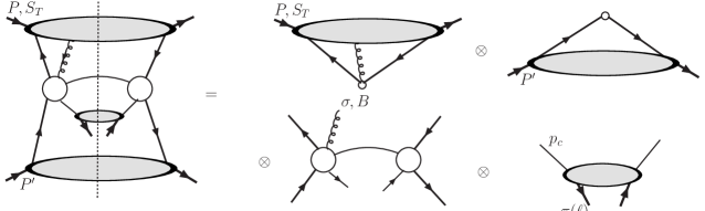
Figure 1: Generic Feynman diagram contributing to the single transverse-spin asymmetry for inclusive pion production in proton-proton scattering at leading twist (twist-three). The polarized cross section can be factorized into convolutions of the following terms: twist-three quark-gluon correlation functions for the transversely polarized proton, parton distributions for the unpolarized proton, pion fragmentation functions, and hard-scattering functions calculable in QCD perturbation theory.

We can think of the contribution in the first line of (5) in terms of the generic Feynman diagram shown in Fig. 1. The upper part of the diagram represents a twist-3 function for the polarized proton, generically given by a three-parton correlation. As was discussed in qs , the dominant contributions to the polarized cross section at forward production angles of the pion are expected from a correlation that connects two quarks and a gluon to the hard-scattering function. We will focus on this particular contribution as well. Other contributions, involving three exchanged gluons gluon , will also exist and play a possibly important role in production at mid-rapidity.

In order to find the field-theoretic expression for the twist-3 function in the first line of Eq. (5), and to derive the rules for computing the associated hard-scattering functions, we consider the diagram in Fig. 2. Here the parts labeled $T_{a}$ and $H_{ab\to c}$ represent the twist-3 function and the partonic hard-scattering, respectively, which are connected by the two independent integrals over the momenta $k_{1}$ and $k_{2}$ that they share. We thus have the following expression for the contribution of the diagram to the spin-dependent cross section:

$$d\Delta\sigma(\ell_{\perp},\vec{s}_{T})\equiv\frac{1}{2S}\sum_{abc}\int\frac{d^{4}k_{1}}{(2\pi)^{4}}\,\frac{d^{4}k_{2}}{(2\pi)^{4}}\,T_{a}(k_{1},k_{2},\vec{s}_{T})\,H_{ab\to c}(k_{1},k_{2},\ell_{\perp})\otimes\phi_{b/B}(x^{\prime})\otimes D_{c\rightarrow h}(z)\ ,$$ (6)

where $1/2S$ is a flux factor and the sum again runs over flavors. In the above expression, spinor, color and Lorentz indices connecting the hard and long-distance parts have already been separated, using the techniques developed in qs , as sketched in Fig. 2. In a covariant gauge, the function $H_{ab\to c}(k_{1},k_{2})$ is contracted with $\left(\frac{2}{N_{C}^{2}-1}\right)(t^{B})_{ij}[(1/2)/{\!\!\!\!P}P_{\sigma}]/(2\pi)$, where the factor $(2\pi)$ is due to the normalization of the twist-3 matrix element $T_{a}$, $N_{C}=3$ is the number of colors, $B$ and $i,j$ are the color indices of the initial gluon and quarks, respectively, and the matrices $(t^{B})_{ij}$ are the SU(3) generators in the fundamental representation.

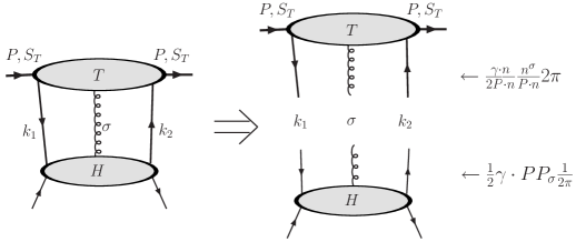
Figure 2: Factorization of hard part and twist-three matrix element: (a) before and (b) after separation of spinor trace and Lorentz indices. For simplicity we have omitted the unpolarized parton distribution and the fragmentation function. $n\sim P^{\prime}$ is a light-like vector with spatial components in direction opposite to those of the initial momentum $P$.

The next step is to perform a “collinear” expansion of the expression for the diagram QS:DYQ . Due to perturbative pinch singularities of the partonic scattering diagrams qs , the integration in Eq. (6) is dominated by the phase space where $k_{i}^{2}\sim 0$, and we can approximate the parton momenta $k_{i}$ entering the hard scattering to be on-shell and nearly parallel to the momentum $P$ of the initial polarized proton:

$$k_{i}^{\mu}=x_{i}P^{\mu}+k^{\mu}_{i,\perp}+k_{i,T}^{2}/(x_{i}S)P^{\prime\mu}\;,$$ (7)

where the $k^{\mu}_{i,\perp}$ are perpendicular to both $P$ and $P^{\prime}$, and where $k_{i,T}^{2}\equiv-(k_{i,\perp}^{\mu})^{2}$. The last term $\propto k_{i,\perp}^{2}$ in (7) can be neglected since it is beyond the order in $k_{i,\perp}$ that we consider. The collinear expansion enables us to reduce the four-dimensional integrals in Eq. (6) to convolutions in the light-cone momentum fractions of the initial partons. Expanding $H_{ab\to c}$ in the partonic momenta, $k_{1}$ and $k_{2}$, around $k_{1}=x_{1}P$ and $k_{2}=x_{2}P$, respectively, we have

$$H_{ab\to c}(k_{1},k_{2})=H_{ab\to c}(x_{1},x_{2}) + \frac{\partial H_{ab\to c}}{\partial k_{1}^{\rho}}(x_{1},x_{2})\left(k_{1}-x_{1}P\right)^{\rho}$$ (8)

$$+ \frac{\partial H_{ab\to c}}{\partial k_{2}^{\rho}}(x_{1},x_{2})\left(k_{2}-x_{2}P\right)^{\rho}+\ldots\ .$$

Because of (7), the derivatives in the latter equation are in the transverse vectors $k^{\mu}_{i,\perp}$ only. The expansion (8), substituted into Eq. (6), allows us to integrate over three of the four components of each of the loop momenta $k_{i}$. The top part of the diagram $T_{a}$ then becomes a twist-three light cone matrix element, given by

$$T_{a,F}(x_{1},x_{2}) = \int\frac{dy_{1}^{-}dy_{2}^{-}}{4\pi}\mbox{e}^{ix_{1}P^{+}y_{1}^{-}+i(x_{2}-x_{1})P^{+}y_{2}^{-}}$$ (9)

$$\quad\times\langle P,\vec{s}_{T}|\bar{\psi}_{a}(0)\gamma^{+}\left[\epsilon^{s_{T}\sigma n\bar{n}}\,F_{\sigma}^{\ +}(y_{2}^{-})\right]\psi_{a}(y_{1}^{-})|P,\vec{s}_{T}\rangle\ ,$$

where we have introduced the subscript “$F$” to indicate that the matrix element involves the gluon field strength tensor $F_{\sigma}^{\ +}$. The additional ordered exponentials of the gauge field that make this matrix element gauge invariant have been suppressed QS:DYQ ; Eq. (9) as it stands is valid in the light-cone gauge $A^{+}=0$. $T_{a,F}$ is a symmetric function of its arguments, $T_{a,F}(x_{1},x_{2})=T_{a,F}(x_{2},x_{1})$.

II.2 Poles in hard-scattering functions and contributions to $k_{\perp}$-expansion

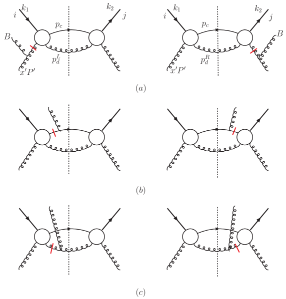
Figure 3: Three classes of quark-gluon scattering diagrams contributing to the spin-dependent cross section $\Delta\sigma(\vec{s}_{T})$: (a) diagrams with an initial-state pole, (b) and (c) diagrams with a final-state pole. Symbols $B$ and $ij$ are color indices for the gluon and the quarks. The propagator that provides the pole is indicated by a bar. All poles shown are “soft-gluon” poles, contributing at $x_{1}=x_{2}$ (see text).

In addition, $T_{a,F}$ is real, implying that the phase needed to generate a single-spin asymmetry has to arise in the functions $H_{ab\to c}$ in Eq. (8). As was shown in qs ; Efremov , imaginary parts in $H_{ab\to c}$ can arise even at tree level, thanks to the pole structure of the hard scattering function. Examples of this are shown in Fig. 3 for the case of quark-gluon scattering. Imaginary parts arise from the scattering amplitude with an extra initial-state gluon when its momentum integral is evaluated by the residues of unpinched poles of the propagators indicated by the bars. The on-shell condition associated with any such pole fixes the momentum fraction of the extra initial-state gluon and hence further simplifies the integrations over the momenta $k_{1}$ and $k_{2}$ in Eq. (6). Roughly speaking, all of the diagrams in Fig. 3 provide an unpinched pole at $x_{1}=x_{2}$, with subtleties that we will address shortly. At these poles, one has qs

$$\frac{\partial H_{ab\to c}}{\partial k^{\rho}_{2,\perp}}(x_{1},x_{2}=x_{1})=-\frac{\partial H_{ab\to c}}{\partial k^{\rho}_{1,\perp}}(x_{1},x_{2}=x_{1})\,.$$ (10)

Thanks to this property, one can organize the calculation of the partonic hard-scattering functions with a simpler momentum flow, using a single transverse momentum $k_{\perp}$, as shown in Fig. 4.

In order to demonstrate the emergence of a strong-interaction phase through a pole contribution at $x_{1}=x_{2}$, let us consider the specific example for the initial-state interaction shown in Fig. 4(a). We need to consider contributions for which the initial-state gluon attaches on the right or on the left side of the cut. The propagator denoted by a bar in the left part of the figure reads

$$\frac{1}{(x^{\prime}P^{\prime}+(x_{2}-x_{1})P+k_{\perp})^{2}+i\epsilon} = \frac{1}{(x_{2}-x_{1})x^{\prime}S+i\epsilon}+{\cal O}(k_{T}^{2})$$ (11)

$$\rightarrow -\frac{i\pi}{x^{\prime}S}\delta(x_{2}-x_{1})\;,$$

where in the second line we have extracted the imaginary part provided by the propagator, which contributes to the single-spin asymmetry. When the gluon attaches on the right-hand side of the cut, we obtain the same result, but with opposite sign. Therefore, effectively the difference of the two diagrams in Fig. 4(a) contributes. The first term on the right-hand side of Eq. (8) cancels in this difference, so that eventually only the other two contribute.

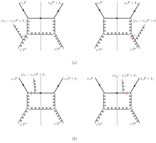
Figure 4: Specific examples of diagrams for generic (a) initial-state and (b) final-state interactions, along with simplified notation of external momenta.

In Eq. (11) we have neglected a term $\propto k_{T}^{2}$ since we are only interested in first-order (linear) $k_{T}$ effects. A linear term is not present in the delta-function in (11) because the vector $k_{\perp}$ is perpendicular to both $P$ and $P^{\prime}$. For final-state interaction, this situation changes. Generic diagrams with final-state interactions involving the “observed” parton are shown in Fig. 4(b). On the left side of the diagram, a phase from the propagator marked by the bar arises as

$$\frac{1}{(\ell/z-(x_{2}-x_{1})P-k_{\perp})^{2}+i\epsilon} = \frac{1}{-2P\cdot\ell\,(x_{2}-x_{1})/z-2\ell\cdot k_{\perp}/z+i\epsilon}+{\cal O}(k_{T}^{2})$$ (12)

$$\rightarrow -\frac{i\pi z}{T}\delta(x_{2}-x_{1}-2\ell\cdot k_{\perp}/T)\;,$$

where the momentum of the fragmenting (“observed”) final-state parton is related to that of the produced hadron by $\ell=zp_{c}$, and $T$ has been defined in Eq. (II). Again, the propagator on the right side of the cut has the same pole, with opposite sign. As Eq. (12) shows, the pole provided by the final-state interactions is located near $x_{1}=x_{2}$, but displaced by a term linear in $k_{\perp}$. When inserted into the collinear expansion (8), this term will make a contribution to the single-spin asymmetry involving a derivative of the delta-function and hence, by partial integration, a derivative of the twist-three quark-gluon correlation function qs .

Such “derivative” terms may, however, also arise in a different way, through the on-shell condition for the unobserved final-state parton. For the diagrams on the left-hand-side of Figs. 4(a) and (b), the momentum carried by that parton is $p_{d}^{L}=x^{\prime}P^{\prime}+x_{2}P+k_{\perp}-\ell/z$, where the superscript $L$ ($R$ introduced later) refers to the diagrams whose extra initial-state gluon is attached to the left (right) of the cut. The phase space provides a delta-function that puts this particle on its mass-shell,

$$\delta\left((p_{d}^{L})^{2}\right) = \delta(x_{2}(x^{\prime}S+T/z)+x^{\prime}U/z-2\ell\cdot k_{\perp}/z)$$ (13)

$$= \frac{1}{x^{\prime}S+T/z}\delta\left(x_{2}-x-\frac{2\ell\cdot k_{\perp}/z}{x^{\prime}S+T/z}\right)\;,$$

where

$$x\equiv\frac{-x^{\prime}U/z}{x^{\prime}S+T/z}\;.$$ (14)

$x$ can be interpreted as the “usual” value of the partonic momentum fraction of the polarized proton if there is no $k_{\perp}$. Eq. (13) fixes $x_{2}$ in terms of the Mandelstam variables $S,T,U$ and a linear term in $k_{\perp}$. The latter will give rise to “derivative” contributions in the same way as Eq. (12) does. If the initial gluon attaches on the right-hand-side of the cut, however, the momentum of the unobserved parton is $p_{d}^{R}=x^{\prime}P^{\prime}+x_{1}P-\ell/z$, and the resulting on-shell condition fixes $x_{1}$:

$$\delta\left((p_{d}^{R})^{2}\right)=\delta(x_{1}-x)\;,$$ (15)

with no dependence on $k_{\perp}$.

Additional contributions to the collinear expansion can of course also arise from terms linear in $k_{\perp}$ in the other “hard” propagators or in the numerator of each diagram. These terms do not lead to “derivative” contributions to the single-spin asymmetry, but to contributions involving $T_{a,F}$ itself.

We close this section with two further observations. First, we note that final-state interactions involving the “unobserved” parton $d$ cancel when summing over contributions where the additional gluon attaches on the right or the left side of the cut. Second, the contributions we have discussed are all characterized by the additional initial gluon becoming soft. The poles arising from this are, therefore, customarily referred to as “soft-gluon poles”. The hard-scattering diagrams will in general possess also other poles, for which an initial quark becomes soft qs . Such “soft-fermion poles” are expected to play a less important role and are not considered in this work.

In the next section, we will provide a “master formula” that allows to take into account all contributions to the $k_{\perp}$-expansion discussed above simultaneously and in a systematic and relatively straightforward manner.

II.3 “Master formula”

As was shown in qs , the factorized expression for $\Delta\sigma(\vec{s}_{T})$ takes the form

$$d\Delta\sigma(\vec{s}_{T}) \propto \frac{1}{2S}\sum_{abc}\int dz\,D_{c\rightarrow h}(z)\int\frac{dx^{\prime}}{x^{\prime}}\,\phi_{b/B}(x^{\prime})\int dx_{1}dx_{2}\,T_{a,F}(x_{1},x_{2})$$ (16)

$$\quad\times i\epsilon^{\rho s_{T}n\bar{n}}\,\lim_{k_{\perp}\to 0}\frac{\partial}{\partial k_{\perp}^{\rho}}H_{ab\rightarrow c}(x_{1},x_{2},x^{\prime},z)\ ,$$

where

$$\epsilon^{\rho s_{T}n\bar{n}}=\epsilon^{\rho\sigma\mu\nu}s_{T\sigma}n_{\mu}n_{\nu}$$ (17)

with $n$ and $\bar{n}$ two light-like vectors whose spatial components are parallel to those of $P^{\prime}$ and $P$, respectively. According to the discussion in the previous section, we are therefore led to consider the following general expression:

$$\lim_{k_{\perp}\to 0}\frac{\partial}{\partial k_{\perp}^{\rho}}\int dx_{1}\int dx_{2}\,T_{a,F}(x_{1},x_{2})\Big{[}\,H_{L}(x_{1},x_{2},k_{\perp})\,\delta(x_{1}-x_{2}+v_{1}\cdot k_{\perp})\delta(x_{2}-x-v_{2}\cdot k_{\perp})$$

$$\hskip 173.56198pt-H_{R}(x_{1},x_{2},k_{\perp})\,\delta(x_{1}-x_{2}+v_{1}\cdot k_{\perp})\delta(x_{1}-x)\Big{]}\;.$$ (18)

Here, $H_{L}$ and $H_{R}$ denote the contributions to $H_{ab\to c}$ for any diagram, when the initial gluon attaches on the left or the right side, respectively. $v_{1}$ and $v_{2}$ are vectors made of $P$, $P^{\prime}$, and $\ell$ whose form follows directly from the preceding discussion. The first delta-function in each of the two terms associated with $H_{L,R}$ results from the propagator poles discussed in Eqs. (11) and (12). For initial-state interactions, $v_{1}=0$ (see Eq. (11)), for final-state ones, $v_{1}=2\ell/T$ (see Eq. (12)). An important point is that $v_{1}$ is the same vector on the left and on the right-hand-side of the cut. The second delta-function in each term results from the on-shell condition for the unobserved particle. As explained earlier, these delta functions differ for the two sides of the cut. We have $v_{2}=2\ell/(x^{\prime}zS+T)$ for the left side and $v_{2}=0$ for the right one, which we have already used.

A straightforward way of dealing with the expression in (II.3) is to use the various delta-functions to perform the integrations over $x_{1}$ and $x_{2}$. This gives:

$$\lim_{k_{\perp}\to 0}\frac{\partial}{\partial k_{\perp}^{\rho}}\Big{[}T_{a,F}(x+(v_{2}-v_{1})\cdot k_{\perp},x+v_{2}\cdot k_{\perp})\,H_{L}(x+(v_{2}-v_{1})\cdot k_{\perp},x+v_{2}\cdot k_{\perp},k_{\perp})$$

$$\hskip 56.9055pt-\,T_{a,F}(x,x+v_{1}\cdot k_{\perp})\,H_{R}(x,x+v_{1}\cdot k_{\perp},k_{\perp})\Big{]}\;.$$ (19)

This term can be organized as

$$(v_{2}-v_{1})_{\rho}\,H_{L}(x,x,0)\,\frac{dT_{a,F}(x,x)}{dx}\,+\,T_{a,F}(x,x)\,\times$$ (20)

$$\times\,\lim_{k_{\perp}\to 0}\frac{\partial}{\partial k_{\perp}^{\rho}}\,\Big{[}H_{L}(x+(v_{2}-v_{1})\cdot k_{\perp},x+v_{2}\cdot k_{\perp},k_{\perp})-H_{R}(x,x+v_{1}\cdot k_{\perp},k_{\perp})\Big{]}_{k_{\perp}=0}\;.$$

This is our “master formula”. In deriving it we have used that the hard-scattering functions with the gluon attaching on the left or the right side of the cut are the same at $k_{\perp}=0$,

$$H_{L}(x,x,0)=H_{R}(x,x,0)\;.$$ (21)

Equation (20) applies to both initial- and final-state interactions. As one can see, the first term is proportional to $dT_{a,F}(x,x)/dx$ [thanks to Eq. (21) it does not matter whether we write $H_{L}(x,x,0)$ or $H_{R}(x,x,0)$ in this term]. This is the “derivative” contribution that we discussed above and that was originally computed in Ref. qs . The second term involves only $T_{a,F}(x,x)$, without a derivative. Equation (20) allows a simultaneous computation of both the derivative and non-derivative contributions.

The next step is to consider all contributing partonic reactions and to calculate the contributions to Eq. (20). The partonic channels we need to consider are $(qg)g\to qg$, $(qg)g\to gq$, $(qg)\bar{q}\to gg$, $(qg)q^{\prime}\to qq^{\prime}$, $(qg)q^{\prime}\to q^{\prime}q$, $(qg)q\to qq$, $(qg)\bar{q}\to q^{\prime}\bar{q}^{\prime}$, $(qg)\bar{q}\to q\bar{q}$, where for each the first two initial partons are entering from the polarized proton via the twist-three correlation function $T_{a,F}$. We remind the reader that we are ignoring contributions involving a three-gluon twist-three correlation function, which would correspond to a $(gg)$ initial state. Crossed channels are implicit and taken into account as well.

Upon calculating all associated hard-scattering functions, we found that they possess a remarkable property: for each process,

$$\lim_{k_{\perp}\to 0}\frac{\partial}{\partial k_{\perp}^{\rho}}\,\Big{[}H_{L}(x+(v_{2}-v_{1})\cdot k_{\perp},x+v_{2}\cdot k_{\perp},k_{\perp})-H_{R}(x,x+v_{1}\cdot k_{\perp},k_{\perp})\Big{]}_{k_{\perp}=0}$$

$$=-\frac{(v_{2}-v_{1})_{\rho}}{x}\,H_{L}(x,x,0)\;,$$ (22)

which is again valid for the case of both initial- and the final-state interactions. We have not been able to develop a proof why Eq. (II.3) holds in general, even though the equation is certainly not accidental and such a proof should be possible. In any case, Equation (II.3) leads to a dramatic simplification of the final result. Inserting (II.3) into (20), one finds the expression

$$-\frac{(v_{2}-v_{1})_{\rho}}{x}\,H_{L}(x,x,0)\,\left[T_{a,F}(x,x)-xT^{\prime}_{a,F}(x,x)\right]\;,$$ (23)

where we have used the short-hand notation $T^{\prime}_{a,F}(x,x)\equiv dT_{a,F}(x,x)/dx$. Thus, even though there could have in principle been two separate hard-scattering functions multiplying $T_{a,F}(x,x)$ and $T^{\prime}_{a,F}(x,x)$, the final result for the combined derivative and non-derivative terms will have a single hard-scattering function for each process, summed over initial- and final-state contributions and multiplying simply the combination $T_{a,F}(x,x)-xT^{\prime}_{a,F}(x,x)$. This hard-scattering function is furthermore identical to the one calculated for the derivative piece in qs . The emerging structure is then very akin to that of the unpolarized cross section. We are now in the position to give the final answer for the single-spin asymmetry.

II.4 Final result

For definiteness, we recall the expressions for the vectors $v_{1}$ and $v_{2}$ introduced above. We have

$$v_{2}=\frac{2\ell}{x^{\prime}zS+T}=-\frac{2p_{c}x}{\hat{u}}\;,$$ (24)

with the partonic Mandelstam variable $\hat{u}=(p_{c}-p^{\prime})^{2}=x^{\prime}U/z$. For initial-state interactions, see Eq. (11), we have $v_{1}=0$, while for final-state ones, see Eq. (12),

$$v_{1}=\frac{2\ell}{T}=\frac{2p_{c}x}{\hat{t}}\;,\;\;\;\mathrm{or}\;\;\;v_{2}-v_{1}=-\frac{2p_{c}x}{\hat{u}}\left(1+\frac{\hat{u}}{\hat{t}}\right)\;,$$ (25)

where $\hat{t}=(p_{c}-p)^{2}=xT/z$.

Using (16) and following the steps presented in detail in Ref. qs , we then find the final expression for the polarized cross section:

$$E_{\ell}\frac{d^{3}\Delta\sigma(\vec{s}_{T})}{d^{3}\ell} = \frac{\alpha_{s}^{2}}{S}\,\sum_{a,b,c}\int_{z_{\rm min}}^{1}\frac{dz}{z^{2}}\,D_{c\to h}(z)\,\int_{x^{\prime}_{\rm min}}^{1}\frac{dx^{\prime}}{x^{\prime}}\,\frac{1}{x^{\prime}S+T/z}\,\phi_{b/B}(x^{\prime})$$

$$\times \sqrt{4\pi\alpha_{s}}\,\left(\frac{\epsilon^{\ell s_{T}n\bar{n}}}{z\hat{u}}\right)\,\frac{1}{x}\left[T_{a,F}(x,x)-x\left(\frac{d}{dx}T_{a,F}(x,x)\right)\right]H_{ab\rightarrow c}(\hat{s},\hat{t},\hat{u})\ ,$$

where $x$ has been defined in Eq. (14), and where

$$x^{\prime}_{\rm min}=\frac{-T/z}{S+U/z}\;,\;\;\;\;\;z_{\rm min}=-\frac{T+U}{S}\;.$$ (27)

The $H_{ab\rightarrow c}$ are the final hard-scattering functions and read

$$H_{ab\rightarrow c}\,=\,H^{I}_{ab\rightarrow c}(\hat{s},\hat{t},\hat{u})+H^{F}_{ab\rightarrow c}(\hat{s},\hat{t},\hat{u})\,\left(1+\frac{\hat{u}}{\hat{t}}\right)\;,$$ (28)

where $H^{I}_{ab\rightarrow c}$ ($H^{F}_{ab\rightarrow c}$) denote the contributions due to the initial-state (final-state) interactions. The factor $(1+\hat{u}/\hat{t})$ results from the expression for $v_{2}-v_{1}$ in Eq. (25). We have collected all $H^{I}_{ab\rightarrow c}$ and $H^{F}_{ab\rightarrow c}$ in Appendix A. Thanks to the structure we have found, they must coincide with the hard-scattering functions calculated for the derivative part in Ref. qs , which they do, up to trivial corrections we found for some of the color factors in qs . The results presented in Appendix A are also in a more compact and transparent notation.

We emphasize again the simplicity of the structure in Eq. (II.4), which is very similar to that of the unpolarized cross section in the denominator of the spin asymmetry. The latter reads:

$$E_{\ell}\frac{d^{3}\sigma}{d^{3}\ell} = \frac{\alpha_{s}^{2}}{S}\,\sum_{a,b,c}\int_{z_{\rm min}}^{1}\frac{dz}{z^{2}}\,D_{c\to h}(z)\,\int_{x^{\prime}_{\rm min}}^{1}\frac{dx^{\prime}}{x^{\prime}}\,\frac{1}{x^{\prime}S+T/z}\,\phi_{b/B}(x^{\prime})$$

$$\times \,\frac{1}{x}\phi_{a/A}(x)\,H^{U}_{ab\rightarrow c}(\hat{s},\hat{t},\hat{u})\ ,$$

with unpolarized hard-scattering functions $H^{U}_{ab\rightarrow c}$ and the usual unpolarized parton distribution functions in hadron $A$, $\phi_{a/A}(x)$. We give the well-known gro $H^{U}_{ab\rightarrow c}$ also in Appendix A.

We finally note that we have written the hard-scattering functions for both the spin-dependent and for the unpolarized case as dimensionless functions. The power-suppression of the single-spin asymmetry is then explicitly visible by the denominator $\hat{u}$ in Eq. (II.4). Furthermore, note the factor $\sqrt{\alpha_{s}}$ in that equation, which results from the additional interaction with a gluon field in the hard-scattering functions for the single-spin case.

III Phenomenological study

We now present some first numerical results for the single-spin asymmetry derived in the previous section. We do not aim at a full-fledged analysis of all the hadronic single-spin data at this point, but would like to examine a few of the salient features of the new RHIC data and of the earlier E704 fixed-target pion production data. We reserve a more detailed analysis to a future publication.

Let us begin by specifying the main ingredients to our calculations. We first remind the reader that all our calculations of the hard-scattering functions are only at the LO level. We therefore use LO parton distribution and fragmentation functions throughout, as well as the one-loop expression for the strong coupling constant. For the unpolarized cross section we use the LO CTEQ5L parton distribution functions cteq5l . Our choice for the fragmentation functions are the LO functions presented in Ref. kretzer . These have the advantage that they provide separate sets for positively and negatively charged pions, which are needed for the comparison to the experimental data.

For the present study, we will make rather simple models for the twist-three quark-gluon correlation functions $T_{a,F}(x,x)$ ($a=u,\bar{u},d,\bar{d},s,\bar{s}$), relating them to their unpolarized leading-twist counterparts. We recall that we do not include any purely gluonic twist-three correlation functions, even though we do take into account the gluon-gluon scattering contribution in the unpolarized cross section in the denominator of $A_{N}$. Our ansatz for the correlation functions is simply:

$$T_{a,F}(x,x,\mu)=N_{a}\,x^{\alpha_{a}}\,(1-x)^{\beta_{a}}\,\phi_{a}(x,\mu)\;,$$ (30)

where $\phi_{a}(x,\mu)$ is the usual twist-two parton distribution for flavor of type $a$ in a proton. Note that we have now written out the dependence of the functions on a factorization scale $\mu$, which we will always choose as $\mu=\ell_{\perp}$. We will in fact assume that the functions $T_{a,F}(x,x,\mu)$ evolve in the same way as the corresponding unpolarized leading-twist distributions. This will certainly not be correct in general, because of the different twist of the two types of distributions, but may be hoped to be a reasonable assumption at the moderate to relatively large $x$ we are interested in here.

We determine the parameters in Eq. (30) through a “global” fit to experimental data for $A_{N}$ as functions of $x_{F}$ defined in Eq. (4), using the expressions in Eqs. (II.4) and (II.4). Here we choose the fixed-target scattering data at $\sqrt{S}\approx 20$ GeV by the E704 experiment E704 for $p^{\uparrow}p\to\pi^{0,\pm}X$ and $\bar{p}^{\uparrow}p\to\pi^{0,\pm}X$, and the latest preliminary RHIC data at $\sqrt{S}=200$ GeV by the STAR star [for $p^{\uparrow}p\to\pi^{0,\pm}X$] and BRAHMS brahms [for $p^{\uparrow}p\to\pi^{\pm}X$ and $p^{\uparrow}p\to K^{\pm}X$] collaborations. The perturbative hard-scattering expression we have derived in the previous section is expected to be only applicable at high transverse momentum, starting from $\ell_{\perp}\gtrsim{\mathrm{a\;few\;GeV}}$. Most of the available data points for $A_{N}$ are at $\ell_{\perp}$-values not much greater than 1 GeV, however. In case of the RHIC data, we always use the correct value for $\ell_{\perp}$ for each data point, keeping however only points with $\ell_{\perp}>1$ GeV. For the E704 data the situation is more complicated as most of the data points have $\ell_{\perp}\lesssim 1$ GeV. In addition, as we discussed in the Introduction, there is generally a problem with the description of even the unpolarized cross sections in the fixed-target regime, when hard-scattering calculations at low orders of perturbation theory are used. All-order resummations resum1 may be very relevant here, which are likely to affect the spin-dependent and the unpolarized cross section in different ways. In view of this, we are tempted to exclude the E704 data from our analysis. On the other hand, the information on single-spin asymmetries is overall still rather sparse, and any information is potentially helpful. In particular, data for anti-proton scattering are only provided by the E704 experiment. Therefore, in order to include the E704 data in the fit, we choose $\ell_{\perp}=1.2$ GeV for these data. In addition, we allow a large shift of the overall normalization of the theory result used for the comparison to these data. This shift is meant to represent in particular the possibly large higher-order effects on $A_{N}$ just described.

We have performed two separate fits to the data. One is a “two-flavor” fit, for which we use only the two valence densities $u_{v}$ and $d_{v}$ in the ansatz (30) and set all other distributions to zero. For this fit we introduce a normalization factor $N_{\mathrm{E704}}=0.5$ for the theory asymmetries in the kinematic region of the E704 data and find:

$${\mathrm{Fit\;I:}\;\;\;\;} N_{u_{v}}=0.275\;,\;\;\;N_{d_{v}}=-0.365\;,$$ (31)

$$\alpha_{u_{v}}=0.508\;,\;\;\;\beta_{u_{v}}=0.399\;,\;\;\;\alpha_{d_{v}}=-0.108\;,\;\;\;\beta_{d_{v}}=0.287\;.$$

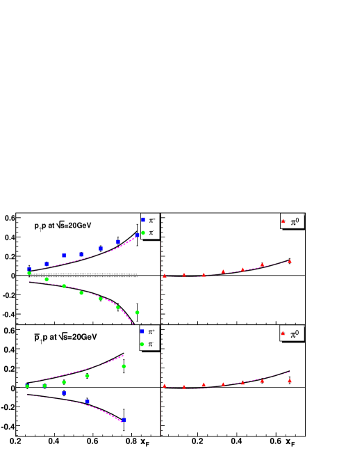
Figure 5: Comparison of the single-spin asymmetries $A_{N}$ using our fit results in Eqs. (30),(31),(33) to the data from E704 E704 . The solid lines are for Fit I (Eq. (31)), and the dashed ones are for Fit II (Eq. (33)). The lower dotted lines in the upper left part of the figure show the contributions to $A_{N}$ for $\pi^{\pm}$ production by the “non-derivative” terms alone, for Fit I. Note that the theory curves in the figure are normalized by $N_{\mathrm{E704}}=0.5$.

The fit has a $\chi^{2}$-value of $304.6$ for the 60 data points and is therefore of rather poor quality. Nonetheless, as one can see from the comparison of the fit to the experimental data shown by the solid lines in Fig. 5 and 6, it has overall the right qualitative features. For example, for $p^{\uparrow}p\to\pi^{+}X$ the asymmetry is positive, which is reflected in a positive valence-$u$ twist-three correlation function emerging from the fit. Likewise, the fact that $A_{N}$ is negative for $p^{\uparrow}p\to\pi^{-}X$ implies a negative valence-$d$ distribution. For anti-proton scattering, the respective asymmetries are then necessarily opposite, because one has qs

$$T_{\bar{a},F}^{\mathrm{anti-proton}}=-T_{a,F}^{\mathrm{proton}}\;.$$ (32)

The asymmetries for $\pi^{0}$ production are between those for $\pi^{+}$ and $\pi^{-}$. The same qualitative features persist to RHIC energies, as can be seen from the comparison to the STAR ($\pi^{0}$) and BRAHMS ($\pi^{\pm}$) data in Fig. 6.

For the second fit, we allow also sea- and anti-quark $T_{F}$ functions. We then find the following parameters:

$${\mathrm{Fit\;II:}\;\;\;\;} N_{u_{v}}=0.353\;,\;\;\;N_{d_{v}}=-0.594\;,$$ (33)

$$N_{\bar{u}}=-N_{\bar{d}}=-N_{u_{\mathrm{sea}}}=N_{d_{\mathrm{sea}}}=-19.8\;,\;\;\;N_{s}=N_{\bar{s}}=-6.63\;,$$

$$\alpha_{u_{v}}=0.696\;,\;\;\;\beta_{u_{v}}=0.559\;,\;\;\;\alpha_{d_{v}}=0.312\;,\;\;\;\beta_{d_{v}}=0.488\;,$$

$$\alpha_{\bar{u}}=\alpha_{u_{\mathrm{sea}}}=\alpha_{\bar{d}}=\alpha_{d_{\mathrm{sea}}}=\alpha_{s}=\alpha_{\bar{s}}=2.91\;,$$

$$\beta_{\bar{u}}=\beta_{u_{\mathrm{sea}}}=\beta_{\bar{d}}=\beta_{d_{\mathrm{sea}}}=\beta_{s}=\beta_{\bar{s}}=0.351\;.$$

Here the relations among the various parameters for sea and anti-quarks are not fit results, but have been imposed. As before, we have a normalization factor $N_{\mathrm{E704}}=0.5$ for the calculated theory asymmetries at the E704 kinematics. The results of this fit are also shown in Figs. 5 and 6, by the dashed lines. One can see that the fit is rather similar to Fit I, but does slightly better. Indeed, the fit has $\chi^{2}=292.6$.

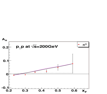
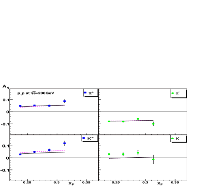
Figure 6: Comparison of the single-spin asymmetries $A_{N}$ using our fit results in Eqs. (30),(31),(33) to the preliminary RHIC data by the STAR star (left) and BRAHMS brahms (right) collaborations. The solid lines are for Fit I (Eq. (31)), and the dashed ones are for Fit II (Eq. (33)). The lower dotted line in the figure shows the contribution to $A_{N}$ by the “non-derivative” terms alone, for Fit I.

While the valence-quark densities completely dominate for the fixed-target case, the sea distributions play a somewhat more significant role at RHIC. We note, however, that in the case of $A_{N}$ in $K^{-}$ production (see Fig. 6) even our fit with a sea distribution does not lead to a significant change in the theoretical result. This is surprising at first sight, because the $K^{-}$ has no valence quarks in common with the proton, so that sea quarks and anti-quarks should be particularly important here. We found that the precise admixture of valence (“favored”), non-valence (“un-favored”), and gluon fragmentation functions is very relevant in this case, as well as that of the hard-scattering functions. We could improve the description of $A_{N}$ in $K^{-}$ production only by assuming a very large negative correlation function $T_{\bar{u},F}$.

We also address the numerical relevance of the “non-derivative” terms that we have calculated in this work. The dotted lines in the upper left part of Fig. 5 and in the left part of Fig. 6 show the contributions to $A_{N}$ that one obtains from the “non-derivative” terms alone, for the case of the two-flavor fit (Fit I). One can see that these contributions are of relatively moderate ($\sim\mathrm{few}\,\%$) size, but non-negligible. They play a bigger role at RHIC energies. There is roughly a 25% increase in the value of $\chi^{2}$ when the “non-derivative” contributions are neglected. Of course, one could refit the $T_{a,F}$ distributions without the “non-derivative” contributions, in which case the theoretical spin asymmetry would be again very close to the dashed or solid lines in the figures. However, we found that such a fit has a slightly worse $\chi^{2}$, and in any case it leads to a fairly different set of $T_{a,F}$ distributions.

In Fig. 7 we show the $T_{a,F}$ distributions that we have found in our fits, for $u$ and $d$ valence- and anti-quarks, at scale $\mu=2$ GeV. The dashed lines are for the “two-flavor” Fit I, while the dotted ones are for Fit II. As one can see, the valence distributions are rather similar in the two fits. Only Fit II has anti-quark distributions. For all distributions, we also show the corresponding unpolarized leading-twist densities, scaled by 1/10 for better visibility.

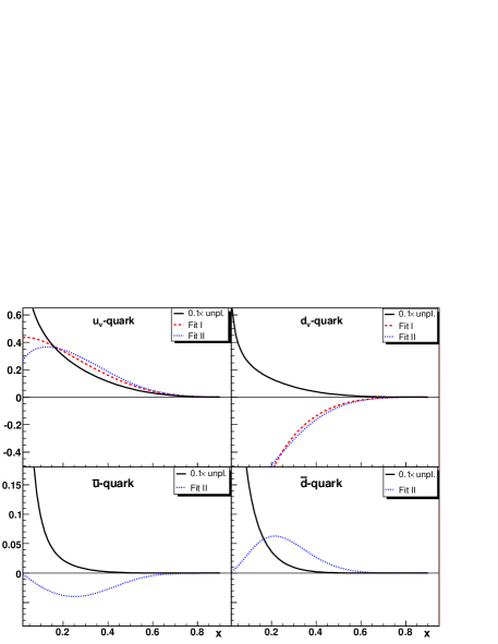
Figure 7: $T_{a,F}$ distributions for $a=u_{v},d_{v},\bar{u},\bar{d}$ resulting from our fits in Eqs. (31) and (33), at scale $\mu=2$ GeV. We also show the corresponding unpolarized parton distribution functions cteq5l , scaled by 1/10.

It is interesting to speculate about the reasons why the overall quality of our fits is relatively poor. We first remind the reader that for the reasons discussed earlier we have rescaled all theory asymmetries in the kinematic region of the E704 data by a factor $1/2$ in the fit. Without the rescaling factor, the total $\chi^{2}$ of the fit would be increased by almost 100 units from the current $\sim 300$, while the sign and the general shape of the asymmetries would still be consistent with the data. Small changes in the normalization of the RHIC data sets do not lead to a very significant further reduction of $\chi^{2}$. We also found that an even better description of all RHIC data is possible if one excludes the E704 data from the fit. Such a fit then tends to badly describe the $A_{N}$ data from E704, even when a normalization factor is applied to the latter. We recall once more that the E704 data are in a kinematic regime where the theoretical calculation of even the unpolarized cross section is challenging, and that we set $\ell_{\perp}=1.2$ GeV for them. It is therefore perhaps not surprising that we find that the consistency of the total data set for $A_{N}$ appears limited. We also caution the reader, however, that much of the RHIC data is still preliminary and one needs to await further experimental information before drawing final conclusions.

Figure 8: (a) Dependence of $A_{N}$ for $\pi^{0}$ production at RHIC at $\sqrt{S}=200$ GeV on $\ell_{\perp}$, for three different values of $x_{F}$. Solid lines are for the $T_{a,F}$ distributions of Fit I, dashed ones are for Fit II. (b) Dependence on $\ell_{\perp}$ for fixed pion pseudo-rapidity $\eta=3.8$ and when taking an average over the bin $3<\eta<4$.

We now use our fitted twist-three correlation functions $T_{a,F}$ of Eqs. (30),(31), and (33) to make a set of further predictions that may be tested at RHIC. The first one concerns the dependence of $A_{N}$ on the produced hadron’s transverse momentum $\ell_{\perp}$. This is a particularly interesting observable, given the power-suppressed nature of $A_{N}$. In fact, as we discussed in the Introduction, $A_{N}$ is expected to decrease as $1/\ell_{\perp}$, at a given $x_{F}$. In Fig. 8(a) we plot $A_{N}$ for $\pi^{0}$ production at $\sqrt{S}=200$ GeV at three fixed values of the Feynman variable, $x_{F}=0.35,\,0.45,\,0.55$, for our two sets of $T_{a,F}$ in Fit I and Fit II. One can clearly see the fall-off with $\ell_{\perp}$. In order to experimentally verify this fall-off, that is, to keep $x_{F}$ fixed while varying $\ell_{\perp}$, one would need to vary the scattering angle. On the other hand, if measurements are made at a (roughly) fixed scattering angle $\theta$ or pseudo-rapidity $\eta=-\ln\tan(\theta/2)$, $x_{F}$ will increase along with $\ell_{\perp}$, as seen from the relation

$$x_{F}=\frac{2\ell_{\perp}}{\sqrt{S}}\sinh(\eta)\;.$$ (34)

This is often the experimentally more relevant situation. As one can see from Fig. 8(a), even though $A_{N}$ decreases with $\ell_{\perp}$ at fixed $x_{F}$, its increase with increasing $x_{F}$ at a given $\ell_{\perp}$ appears to be stronger. Hence, one expects that for measurements at fixed scattering angle $A_{N}$ will actually increase with $\ell_{\perp}$. Indeed, this is the case, as shown in Fig. 8(b). If one averages experimentally over a bin of forward rapidities, say, $3<\eta<4$, the increase of $A_{N}$ with $\ell_{\perp}$ is less pronounced but still there. Another observable, most relevant to measurements at STAR cross_star , is the dependence on the asymmetry on the pion energy $E_{\pi}=\ell_{\perp}\,\cosh(\eta)$ for fixed $\eta$. This is plotted in Fig. 9 for our two fits, for the cases $\eta=3.3$ and $\eta=3.8$.

Figure 9: (a) Dependence of $A_{N}$ for $\pi^{0}$ production at RHIC at $\sqrt{S}=200$ GeV on the pion energy $E_{\pi}$, for fixed $\eta=3.3$ and $\eta=3.8$. Solid lines are for the $T_{a,F}$ distributions of Fit I, dashed ones are for Fit II.

It is also interesting to consider the energy dependence of $A_{N}$. So far, we have data from fixed-target scattering at $\sqrt{S}\sim 20$ GeV and from RHIC at a center-of-mass energy about an order of magnitude higher. In order to shed further light on the mechanisms responsible for the large observed values of $A_{N}$ at these two energies, information at an intermediate energy will be particularly useful. In the 2006 run, data have been taken at RHIC at $\sqrt{S}=62.4$ GeV. Using our above fit results, we find the theoretical expectations for $A_{N}$ for $\pi^{\pm}$ and $\pi^{0}$ production as functions of $x_{F}$ shown in Fig. 10. We have for now again correlated $x_{F}$ and $\ell_{\perp}$ through Eq. (34) at fixed pseudo-rapidity $\eta=3.3$. Clearly, comparison to eventual data will require implementation of the correct kinematics. In the figure, we compare results for $\sqrt{S}=62.4$ GeV and 200 GeV. One can see that, at fixed $x_{F}$ and $\eta$, a significant increase of $A_{N}$ with energy should be expected.

Figure 10: Comparison of $A_{N}$ for $\pi^{\pm}$ and $\pi^{0}$ production as functions of $x_{F}$ at $\sqrt{S}=62.4$ and at 200 GeV, using our two fit results. We have chosen a fixed pion pseudo-rapidity $\eta=3.3$.

We finally briefly turn to processes other than inclusive-hadron production. We first consider the spin asymmetry in single-inclusive jet production. The partonic hard-scattering functions for this case are the same as for hadron production, but there are no fragmentation functions here. The result for $A_{N}$ for jet-production at RHIC at forward $x_{F}$ and fixed $\eta=3.3$ is shown in Fig. 11. For comparison, we also show again the corresponding curve for $\pi^{0}$ production for Fit I. One can see that essentially the asymmetry for jets is shifted by a factor $\sim 2$ to the right with respect to that for pions. This can be understood from the fact that in the kinematic regime relevant here a pion takes on average roughly 50% of a fragmenting parton’s energy strik , whereas all of the energy goes into a jet.

Figure 11: Single-spin asymmetry for jet production (with transverse momentum $\ell_{\perp}>3$ GeV) at RHIC at $\sqrt{S}=200$ GeV, as a function of $x_{F}$ for fixed pseudo-rapidity $\eta=3.3$. We show the results for both Fit I (solid) and Fit II (dashed). The dotted curve shows the same for $\pi^{0}$ production for Fit I.

Another process of interest is prompt-photon production. Photons are generally much less copiously produced at RHIC energies than pions, which results in larger statistical uncertainties on the spin asymmetries. However, given the progress on luminosity and polarization at RHIC, first measurements of $A_{N}$ for prompt photons should become possible in the near-term future. Photons have the advantage that one important production mechanism is quark-gluon Compton scattering, $qg\to\gamma q$, with the reaction $q\bar{q}\to\gamma g$ yielding a smaller contribution. In addition, in these processes the photon couples in a “direct” (or, point-like) way, that is, there are no fragmentation functions involved. Photons can, however, also be produced in jet fragmentation owens . The relative importance of the “direct” and the fragmentation contributions depends on kinematics, but also on aspects of the experimental measurement. It is possible, for example, to largely suppress the fragmentation contribution by a so-called photon isolation cut owens . In the following, in order to obtain first estimates, we will calculate the single-spin asymmetry for prompt photons based on either the “direct” contributions alone, or on the sum of the “direct” and the full fragmentation contributions. The former is more representative of the asymmetry for an isolated photon cross section, while the latter corresponds to a fully inclusive measurement. When data will become available, a more careful theoretical analysis will clearly become necessary.

Predictions for $A_{N}$ for prompt-photon production can then be obtained from Eq. (II.4) by using the appropriate hard-scattering functions for the reactions $(qg)g\to\gamma q$ and $(qg)\bar{q}\to\gamma g$ and by replacing the coupling factor $\alpha_{s}^{2}$ by $\alpha_{s}\,\alpha_{\mathrm{e.m.}}\,e_{q}^{2}$, where $\alpha_{\mathrm{e.m.}}$ is the electromagnetic coupling constant and $e_{q}$ is the fractional electric charge carried by the quark of flavor $q$. We give the resulting expressions in Appendix B, along with the corresponding ones for the unpolarized case, to be used in Eq. (II.4), with the same replacement of the couplings. Taking the fit results of

Figure 12: Single-spin asymmetry for prompt-photon production at RHIC at $\sqrt{S}=200$ GeV, as a function of $x_{F}$ for fixed pseudo-rapidity $\eta=3.3$. We show the predictions for both Fit I (solid) and Fit II (dashed). We show separately the results for the cases when the fragmentation component is taken into account or neglected. The dotted curve shows the earlier result for $\pi^{0}$ production for Fit I.

Eqs. (30),(31),(33) we obtain the predictions shown in Fig. 12, which are for $\sqrt{S}=200$ GeV. Again we have chosen a fixed pseudo-rapidity $\eta=3.3$. For comparison we also show again the corresponding result for $A_{N}$ for $\pi^{0}$ production. The differences between the asymmetries for photons (“direct only”) and $\pi^{0}$ are quite striking. They mostly result from a rather different structure of the corresponding hard-scattering functions (see Eqs. (36) and (43) in Appendices A and B, respectively) and are therefore a real prediction of the formalism. One also sees that the two fits I and II give somewhat different predictions for $A_{N}$ for the photons “direct only” case. This is due to the contributions from $(\bar{q}g)q$ scattering which are present for Fit II, but absent for fit I since for this fit we assumed that the sea quark $T_{a,F}$ functions vanish.

When the fragmentation contribution to the prompt photon cross section is taken into account, the single-spin asymmetry becomes much more like the one for $\pi^{0}$, at least for the lower $x_{F}$. The reason is that in the kinematic regime relevant here, i.e. at relatively low transverse momenta $\ell_{\perp}$, the fragmentation component actually dominates the cross section. Future measurements of the single-spin asymmetry for isolated photons should see an asymmetry close to the lower one (“direct only”) in Fig. 12, while for the fully inclusive (non-isolated) case $A_{N}$ should be smaller and closer to that for $\pi^{0}$ production.

IV Conclusions and outlook

We have presented a new study of the single-spin asymmetry in single-inclusive hadron production in hadronic scattering. The importance of this asymmetry lies in the new insights into nucleon structure it may provide, but also in the challenge that its description poses for QCD theory due its power-suppressed nature. We have extend the previous calculations in qs by deriving also the so-called “non-derivative” contributions to the spin-dependent cross section. We have found that these combine with the “derivative” pieces into a remarkably simple structure.

Using our derived cross section, we have also made first phenomenological studies, using the E704 fixed-target and the latest preliminary RHIC (STAR and BRAHMS) data. We have found that a simultaneous description of all these data is possible, albeit at a more qualitative, than quantitative, level, with the RHIC data overall better described. The “non-derivative” contributions we have calculated are of moderate importance.

We have finally made predictions for a number of other single-spin observables at RHIC, in particular for the $\ell_{\perp}$-dependence of $A_{N}$ for $\pi^{0}$ production, for scattering at 62.4 GeV, and for the asymmetries for single-jet and prompt-photon final states.

For the future, it will be desirable to extend our work in a number of ways. Regarding the theoretical framework, one should eventually include also purely gluonic higher-twist correlation functions. These are expected to be of particular relevance for the spin asymmetry at mid-rapidity, which was found experimentally to be small phenix . Also, we have so far only considered the “soft-gluon” contributions to the spin asymmetry, for which the gluon in the twist-three quark-gluon correlation function is soft. As we mentioned earlier, there are also in general “soft-fermion” contributions. These involve, among other things, the functions $T_{a,F}(x,0)$, rather than the $T_{a,F}(x,x)$ that we found for the soft-gluon case. The soft-fermion contributions have their own hard-scattering functions and may make a significant contribution to the spin asymmetry as well. Further points of interest will be the evolution of the functions $T_{a,F}(x,x)$, and the detailed study of similarities and differences between our approach and the formalism of ams , where the spin asymmetry in the process $p^{\uparrow}p\to\pi\pi X$ has been considered in the context of gauge links in hard-scattering processes. This could be achieved for example by a study of the single-spin asymmetry for two-pion or two-jet production in the framework of qs that we have used here.

Regarding phenomenology, our studies so far have a more illustrative character. With new experimental information arriving from RHIC, however, we will be entering an era where detailed global analyses of the data on $A_{N}$ will become possible.

Appendix A: Hard-scattering functions for inclusive-hadron production

In this Appendix we list the hard-scattering functions relevant for single-inclusive hadron production. For each partonic channel, we give the functions $H^{I}_{ab\rightarrow c}$ and $H^{F}_{ab\rightarrow c}$, which are to be used in Eq. (28). We also present the corresponding unpolarized cross sections $H^{U}_{ab\rightarrow c}$ for Eq. (II.4). We have:

$qg\to qg$ scattering:

$$H^{U}_{qg\rightarrow q}(\hat{s},\hat{t},\hat{u}) = \frac{C_{F}}{N_{C}}\left[-\frac{\hat{s}}{\hat{u}}-\frac{\hat{u}}{\hat{s}}\right]\;\left[1-\frac{N_{C}}{C_{F}}\frac{\hat{s}\hat{u}}{\hat{t}^{2}}\right]\;,$$

$$H^{I}_{qg\rightarrow q}(\hat{s},\hat{t},\hat{u}) = \frac{1}{2(N_{C}^{2}-1)}\left[-\frac{\hat{s}}{\hat{u}}-\frac{\hat{u}}{\hat{s}}\right]\;\left[1-N_{C}^{2}\frac{\hat{u}^{2}}{\hat{t}^{2}}\right]\;,$$

$$H^{F}_{qg\rightarrow q}(\hat{s},\hat{t},\hat{u}) = \frac{1}{2N_{C}^{2}(N_{C}^{2}-1)}\left[-\frac{\hat{s}}{\hat{u}}-\frac{\hat{u}}{\hat{s}}\right]\;\left[1+2N_{C}^{2}\frac{\hat{s}\hat{u}}{\hat{t}^{2}}\right]\;.$$ (35)

$qg\to gq$ scattering:

$$H^{U}_{qg\rightarrow g}(\hat{s},\hat{t},\hat{u}) = \frac{C_{F}}{N_{C}}\left[-\frac{\hat{s}}{\hat{t}}-\frac{\hat{t}}{\hat{s}}\right]\;\left[1-\frac{N_{C}}{C_{F}}\frac{\hat{s}\hat{t}}{\hat{u}^{2}}\right]\;,$$

$$H^{I}_{qg\rightarrow g}(\hat{s},\hat{t},\hat{u}) = \frac{1}{2(N_{C}^{2}-1)}\left[-\frac{\hat{s}}{\hat{t}}-\frac{\hat{t}}{\hat{s}}\right]\;\left[1-N_{C}^{2}\frac{\hat{t}^{2}}{\hat{u}^{2}}\right]\;,$$

$$H^{F}_{qg\rightarrow g}(\hat{s},\hat{t},\hat{u}) = -\frac{1}{2(N_{C}^{2}-1)}\left[-\frac{\hat{s}}{\hat{t}}-\frac{\hat{t}}{\hat{s}}\right]\;\left[1-N_{C}^{2}\frac{\hat{s}^{2}}{\hat{u}^{2}}\right]\;.$$ (36)

$q\bar{q}\to gg$ scattering:

$$H^{U}_{q\bar{q}\rightarrow g}(\hat{s},\hat{t},\hat{u}) = \frac{2C_{F}^{2}}{N_{C}}\left[\frac{\hat{t}}{\hat{u}}+\frac{\hat{u}}{\hat{t}}\right]\left[1-\frac{N_{C}}{C_{F}}\frac{\hat{t}\hat{u}}{\hat{s}^{2}}\right]\;,$$

$$H^{I}_{q\bar{q}\rightarrow g}(\hat{s},\hat{t},\hat{u}) = -\frac{1}{2N_{C}^{3}}\left[\frac{\hat{t}}{\hat{u}}+\frac{\hat{u}}{\hat{t}}\right]\left[1+2N_{C}^{2}\frac{\hat{t}\hat{u}}{\hat{s}^{2}}\right]\;,$$

$$H^{F}_{q\bar{q}\rightarrow g}(\hat{s},\hat{t},\hat{u}) = -\frac{1}{2N_{C}}\left[\frac{\hat{t}}{\hat{u}}+\frac{\hat{u}}{\hat{t}}\right]\left[1-N_{C}^{2}\frac{\hat{u}^{2}}{\hat{s}^{2}}\right]\;.$$ (37)

$qq^{\prime}\to qq^{\prime}$ scattering:

$$H^{U}_{qq^{\prime}\rightarrow q}(\hat{s},\hat{t},\hat{u}) = \frac{C_{F}}{N_{C}}\left[\frac{\hat{s}^{2}+\hat{u}^{2}}{\hat{t}^{2}}\right]\;,$$

$$H^{I}_{qq^{\prime}\rightarrow q}(\hat{s},\hat{t},\hat{u}) = -\frac{1}{N_{C}^{2}}\left[\frac{\hat{s}^{2}+\hat{u}^{2}}{\hat{t}^{2}}\right]\;,$$

$$H^{F}_{qq^{\prime}\rightarrow q}(\hat{s},\hat{t},\hat{u}) = -\frac{1}{2N_{C}^{2}}\left[\frac{\hat{s}^{2}+\hat{u}^{2}}{\hat{t}^{2}}\right]\;.$$ (38)

$qq^{\prime}\to q^{\prime}q$ scattering:

$$H^{U}_{qq^{\prime}\rightarrow q^{\prime}}(\hat{s},\hat{t},\hat{u}) = \frac{C_{F}}{N_{C}}\left[\frac{\hat{s}^{2}+\hat{t}^{2}}{\hat{u}^{2}}\right]\;,$$

$$H^{I}_{qq^{\prime}\rightarrow q^{\prime}}(\hat{s},\hat{t},\hat{u}) = -\frac{1}{N_{C}^{2}}\left[\frac{\hat{s}^{2}+\hat{t}^{2}}{\hat{u}^{2}}\right]\;,$$

$$H^{F}_{qq^{\prime}\rightarrow q^{\prime}}(\hat{s},\hat{t},\hat{u}) = \frac{N_{C}^{2}-2}{2N_{C}^{2}}\left[\frac{\hat{s}^{2}+\hat{t}^{2}}{\hat{u}^{2}}\right]\;.$$ (39)

$qq\to qq$ scattering:

$$H^{U}_{qq\rightarrow q}(\hat{s},\hat{t},\hat{u}) = \frac{C_{F}}{N_{C}}\left[\frac{\hat{s}^{2}+\hat{u}^{2}}{\hat{t}^{2}}+\frac{\hat{s}^{2}+\hat{t}^{2}}{\hat{u}^{2}}-\frac{2}{N_{C}}\frac{\hat{s}^{2}}{\hat{t}\hat{u}}\right]\;,$$

$$H^{I}_{qq\rightarrow q}(\hat{s},\hat{t},\hat{u}) = -\frac{1}{N_{C}^{2}}\left[\frac{\hat{s}^{2}+\hat{u}^{2}}{\hat{t}^{2}}+\frac{\hat{s}^{2}+\hat{t}^{2}}{\hat{u}^{2}}-\frac{N_{C}^{2}+1}{N_{C}}\frac{\hat{s}^{2}}{\hat{t}\hat{u}}\right]\;,$$

$$H^{F}_{qq\rightarrow q}(\hat{s},\hat{t},\hat{u}) = -\frac{1}{2N_{C}^{2}}\left[\frac{\hat{s}^{2}+\hat{u}^{2}}{\hat{t}^{2}}\right]+\frac{N_{C}^{2}-2}{2N_{C}^{2}}\left[\frac{\hat{s}^{2}+\hat{t}^{2}}{\hat{u}^{2}}\right]+\frac{1}{N_{C}^{3}}\frac{\hat{s}^{2}}{\hat{t}\hat{u}}\;.$$ (40)

$q\bar{q}\to q^{\prime}\bar{q}^{\prime}$ scattering:

$$H^{U}_{q\bar{q}\rightarrow q^{\prime}}(\hat{s},\hat{t},\hat{u}) = \frac{C_{F}}{N_{C}}\left[\frac{\hat{t}^{2}+\hat{u}^{2}}{\hat{s}^{2}}\right]\;,$$

$$H^{I}_{q\bar{q}\rightarrow q^{\prime}}(\hat{s},\hat{t},\hat{u}) = \frac{1}{2N_{C}^{2}}\left[\frac{\hat{t}^{2}+\hat{u}^{2}}{\hat{s}^{2}}\right]\;,$$

$$H^{F}_{q\bar{q}\rightarrow q^{\prime}}(\hat{s},\hat{t},\hat{u}) = \frac{N_{C}^{2}-2}{2N_{C}^{2}}\left[\frac{\hat{t}^{2}+\hat{u}^{2}}{\hat{s}^{2}}\right]\;.$$ (41)

$q\bar{q}\to q\bar{q}$ scattering:

$$H^{U}_{q\bar{q}\rightarrow q}(\hat{s},\hat{t},\hat{u}) = \frac{C_{F}}{N_{C}}\left[\frac{\hat{t}^{2}+\hat{u}^{2}}{\hat{s}^{2}}+\frac{\hat{s}^{2}+\hat{u}^{2}}{\hat{t}^{2}}-\frac{2}{N_{C}}\frac{\hat{u}^{2}}{\hat{s}\hat{t}}\right]\;,$$

$$H^{I}_{q\bar{q}\rightarrow q}(\hat{s},\hat{t},\hat{u}) = -\frac{N_{C}^{2}-2}{2N_{C}^{2}}\frac{\hat{s}^{2}+\hat{u}^{2}}{\hat{t}^{2}}+\frac{1}{2N_{C}^{2}}\frac{\hat{t}^{2}+\hat{u}^{2}}{\hat{s}^{2}}-\frac{1}{N_{C}^{3}}\frac{\hat{u}^{2}}{\hat{s}\hat{t}}\;,$$

$$H^{F}_{q\bar{q}\rightarrow q}(\hat{s},\hat{t},\hat{u}) = -\frac{1}{2N_{C}^{2}}\left[\frac{\hat{s}^{2}+\hat{u}^{2}}{\hat{t}^{2}}\right]+\frac{N_{C}^{2}-2}{2N_{C}^{2}}\left[\frac{\hat{t}^{2}+\hat{u}^{2}}{\hat{s}^{2}}\right]+\frac{1}{N_{C}^{3}}\frac{\hat{u}^{2}}{\hat{s}\hat{t}}\;,$$ (42)

where $C_{F}=(N_{C}^{2}-1)/2N_{C}=4/3$.

Appendix B: Hard-scattering functions for direct-photon production

In this Appendix we list the hard-scattering functions relevant for single-inclusive prompt-photon production. In this case, there are only initial-state contributions $H^{I}_{ab\rightarrow\gamma}$ in Eq. (28). For convenience, we also again give the unpolarized contributions $H^{U}_{ab\rightarrow\gamma}$. We have:

$qg\to\gamma q$ scattering:

$$H^{U}_{qg\rightarrow\gamma}(\hat{s},\hat{t},\hat{u}) = \frac{e_{q}^{2}}{N_{C}}\left[-\frac{\hat{s}}{\hat{t}}-\frac{\hat{t}}{\hat{s}}\right]\;,$$

$$H^{I}_{qg\rightarrow\gamma}(\hat{s},\hat{t},\hat{u}) = e_{q}^{2}\frac{N_{C}}{N_{C}^{2}-1}\left[-\frac{\hat{s}}{\hat{t}}-\frac{\hat{t}}{\hat{s}}\right]\;.$$ (43)

$q\bar{q}\to\gamma g$ scattering:

$$H^{U}_{q\bar{q}\rightarrow\gamma}(\hat{s},\hat{t},\hat{u}) = e_{q}^{2}\frac{2C_{F}}{N_{C}}\left[\frac{\hat{t}}{\hat{u}}+\frac{\hat{u}}{\hat{t}}\right]\;,$$

$$H^{I}_{q\bar{q}\rightarrow\gamma}(\hat{s},\hat{t},\hat{u}) = -e_{q}^{2}\frac{1}{N_{C}^{2}}\left[\frac{\hat{t}}{\hat{u}}+\frac{\hat{u}}{\hat{t}}\right]\;.$$ (44)

References

- (1) D. L. Adams et al. [E581 and E704 Collaborations], Phys. Lett. B 261, 201 (1991); D. L. Adams et al. [FNAL-E704 Collaboration], Phys. Lett. B 264, 462 (1991); K. Krueger et al., Phys. Lett. B 459, 412 (1999).
- (2) J. Adams et al. [STAR Collaboration], Phys. Rev. Lett. 92, 171801 (2004) [arXiv:hep-ex/0310058]; C. A. Gagliardi [STAR Collaboration], talk presented at the “14th International Workshop on Deep Inelastic Scattering (DIS 2006)”, Tsukuba, Japan, April 20-24, 2006, arXiv:hep-ex/0607003.
- (3) S. S. Adler [PHENIX Collaboration], Phys. Rev. Lett. 95, 202001 (2005) [arXiv:hep-ex/0507073]; K. Tanida [PHENIX Collaboration], talk presented at the “14th International Workshop on Deep Inelastic Scattering (DIS 2006)”, Tsukuba, Japan, April 20-24, 2006; C. A. Aidala, Ph.D. Thesis, Columbia U., arXiv:hep-ex/0601009.
- (4) F. Videbaek [BRAHMS Collaboration], AIP Conf. Proc. 792, 993 (2005) [arXiv:nucl-ex/0508015]; J. H. Lee [BRAHMS Collaboration], talk presented at the “14th International Workshop on Deep Inelastic Scattering (DIS 2006)”, Tsukuba, Japan, April 20-24, 2006.
- (5) J. P. Ralston and D. E. Soper, Nucl. Phys. B 152, 109 (1979); R. L. Jaffe and X. Ji, Nucl. Phys. B 375, 527 (1992).
- (6) G. L. Kane, J. Pumplin and W. Repko, Phys. Rev. Lett. 41, 1689 (1978).
- (7) J. W. Qiu and G. Sterman, Phys. Rev. Lett. 67, 2264 (1991); Nucl. Phys. B 378, 52 (1992); Phys. Rev. D 59, 014004 (1999) [arXiv:hep-ph/9806356].
- (8) A. V. Efremov and O. V. Teryaev, Sov. J. Nucl. Phys. 36, 140 (1982) [Yad. Fiz. 36, 242 (1982)]; A. V. Efremov and O. V. Teryaev, Phys. Lett. B 150, 383 (1985).
- (9) Y. Kanazawa and Y. Koike, Phys. Lett. B 478, 121 (2000) [arXiv:hep-ph/0001021]; Phys. Lett. B 490, 99 (2000) [arXiv:hep-ph/0007272].
- (10) D. W. Sivers, Phys. Rev. D 41, 83 (1990); Phys. Rev. D 43, 261 (1991).
- (11) M. Anselmino, M. Boglione and F. Murgia, Phys. Lett. B 362, 164 (1995) [arXiv:hep-ph/9503290]; M. Anselmino and F. Murgia, Phys. Lett. B 442, 470 (1998) [arXiv:hep-ph/9808426]; U. D’Alesio and F. Murgia, Phys. Rev. D 70, 074009 (2004) [arXiv:hep-ph/0408092]; M. Anselmino, U. D’Alesio, S. Melis and F. Murgia, arXiv:hep-ph/0608211.
- (12) X. Ji, J. W. Qiu, W. Vogelsang and F. Yuan, Phys. Rev. Lett. 97, 082002 (2006) [arXiv:hep-ph/0602239]; Phys. Rev. D 73, 094017 (2006) [arXiv:hep-ph/0604023]; Phys. Lett. B 638, 178 (2006) [arXiv:hep-ph/0604128].
- (13) J. Adams et al. [STAR Collaboration], arXiv:nucl-ex/0602011; F. Simon [STAR Collaboration], arXiv:hep-ex/0608050.
- (14) S. S. Adler et al. [PHENIX Collaboration], Phys. Rev. Lett. 91, 241803 (2003) [arXiv:hep-ex/0304038]; Y. Fukao [PHENIX Collaboration], talk presented at the “14th International Workshop on Deep Inelastic Scattering (DIS 2006)”, Tsukuba, Japan, April 20-24, 2006.
- (15) R. Debbe [BRAHMS Collaboration], arXiv:nucl-ex/0608040.
- (16) P. Aurenche, M. Fontannaz, J. P. Guillet, B. A. Kniehl and M. Werlen, Eur. Phys. J. C 13, 347 (2000) [arXiv:hep-ph/9910252]; C. Bourrely and J. Soffer, Eur. Phys. J. C 36, 371 (2004) [arXiv:hep-ph/0311110].
- (17) D. de Florian and W. Vogelsang, Phys. Rev. D 71, 114004 (2005).
- (18) X. D. Ji, Phys. Lett. B 289, 137 (1992).
- (19) J. W. Qiu and G. Sterman, Nucl. Phys. B 353, 105 (1991); Nucl. Phys. B 353, 137 (1991).
- (20) B. L. Combridge, J. Kripfganz and J. Ranft, Phys. Lett. B 70, 234 (1977); R. Cutler and D. W. Sivers, Phys. Rev. D 17, 196 (1978); J. F. Owens, E. Reya and M. Gluck, Phys. Rev. D 18, 1501 (1978).
- (21) H. L. Lai et al. [CTEQ Collaboration], Eur. Phys. J. C 12, 375 (2000) [arXiv:hep-ph/9903282].
- (22) S. Kretzer, Phys. Rev. D 62, 054001 (2000) [arXiv:hep-ph/0003177].
- (23) V. Guzey, M. Strikman and W. Vogelsang, Phys. Lett. B 603, 173 (2004) [arXiv:hep-ph/0407201]; S. Kretzer, Acta Phys. Polon. B 36, 179 (2005) [arXiv:hep-ph/0410219].
- (24) for discussion, see: J. F. Owens, Rev. Mod. Phys. 59, 465 (1987); E. L. Berger and J. W. Qiu, Phys. Rev. D 44, 2002 (1991); W. Vogelsang and M. R. Whalley, J. Phys. G 23, A1 (1997).
- (25) C. J. Bomhof, P. J. Mulders and F. Pijlman, Phys. Lett. B 596, 277 (2004) [arXiv:hep-ph/0406099]; A. Bacchetta, C. J. Bomhof, P. J. Mulders and F. Pijlman, Phys. Rev. D 72, 034030 (2005) [arXiv:hep-ph/0505268]; C. J. Bomhof, P. J. Mulders and F. Pijlman, Eur. Phys. J. C 47, 147 (2006) [arXiv:hep-ph/0601171]; see, in particular, C. J. Bomhof and P. J. Mulders, arXiv:hep-ph/0609206.