Gluonic Pole Cross Sections and Single Spin Asymmetries
in Hadron-Hadron Scattering

Abstract

The gauge-links connecting the parton field operators in the hadronic matrix elements appearing in the transverse momentum dependent distribution functions give rise to $T$-odd effects. Due to the process-dependence of the gauge-links the $T$-odd distribution functions appear with different prefactors. A consequence is that in the description of single spin asymmetries the parton distribution and fragmentation functions are convoluted with gluonic pole cross sections rather than the basic partonic cross sections. In this paper we calculate the gluonic pole cross sections encountered in single spin asymmetries in hadron-hadron scattering. The case of back-to-back pion production in polarized proton-proton scattering is worked out explicitly. It is shown how $T$-odd gluon distribution functions originating from gluonic pole matrix elements appear in twofold.

I Introduction

In recent years there has been increasing interest in the theoretical description of single spin asymmetries (SSA), which in some processes can grow to several tens of percents in certain kinematical regimes Adams et al. (1991a, b); Bravar et al. (1996); Airapetian et al. (2001); Adler et al. (2003); Adams et al. (2004); Airapetian et al. (2005). Single spin asymmetries have a characteristic behavior under time reversal, being time-reversal odd ($T$-odd). Interest has increased chiefly because SSA may provide the simplest access to the transverse spin distribution function of quarks in nucleons, which cannot be probed in inclusive (polarized) deep inelastic scattering. The chiral-odd nature of the transverse spin distribution requires a scattering process with at least two observed hadrons. For spin 0 and spin $\frac{1}{2}$ hadrons, the $T$-odd effects require measurement of azimuthal asymmetries in which the quark transverse momentum plays a role. The $T$-odd effects vanish upon integration over the transverse momentum, but not in transverse momentum weighted functions. These are referred to as transverse moments and typically show up in the description of azimuthal spin asymmetries. Describing distribution functions in terms of hadronic matrix elements, the $T$-odd effects come from the gauge-links that connect the parton field operators. The gauge-links are path-ordered exponentials that ensure the gauge-invariance of the bilocal products of parton field operators. In transverse momentum integrated correlators the nonlocality is along a lightlike direction. The integration path in the gauge-link runs along this lightlike direction and can be calculated by resumming all exchanges of collinear gluons between the hadronic remnants and the hard part. In transverse momentum dependent (TMD) correlators the nonlocality is not restricted to a lightlike direction, but rather to a light-front. It turns out that the integration path of the gauge-link between the two parton fields, which in this case involves resumming collinear and transverse gluon interactions Belitsky et al. (2003); Boer et al. (2003), depends on the hard partonic subprocess. In particular it depends on the color-flow through the subprocess.

The time-reversal odd effects for fragmentation functions do not have such a clear origin, since their description in terms of matrix elements of parton field operators is more complicated. In 1993 a mechanism was identified by Collins to generate $T$-odd effects in the final-state Collins (1993). This mechanism originates from final state interactions between an outgoing observed hadron and the accompanying jet. Due to the explicit appearance of out-states, time-reversal symmetry does not constrain the parametrization of the fragmentation correlators. Hence, $T$-odd fragmentation effects arise from both final-state interactions and gauge-links.

Since there are no corresponding effects for the in-states on the distribution side, no $T$-odd effects were expected in the distribution correlators. This expectation was falsified by Brodsky, Hwang and Schmidt, who could produce leading order single spin asymmetries in a model calculation, coming from the soft gluon interactions Brodsky et al. (2002a). The effect is identified with the nontrivial behavior of the gauge-link under time reversal, in particular for the case of TMD correlators where they have both longitudinal and transverse parts. In the lightcone gauge the connection could be made to the gluonic pole matrix elements in the Qiu-Sterman mechanism Boer et al. (2003), which is known to generate single spin asymmetries in the collinear description of hard processes Qiu and Sterman (1999).

In the simplest hadronic scattering processes, such as semi-inclusive deep inelastic scattering (SIDIS), Drell-Yan (DY) scattering and $e^{+}e^{-}$-annihilation, only a limited number of different gauge-link structures appear. These are the well-known future and past-pointing Wilson-lines. They are related by time-reversal and, correspondingly, the $T$-odd distribution functions appear with opposite sign. When going beyond these processes one may encounter more complicated gauge-link structures Bomhof et al. (2004); Bacchetta et al. (2005); Bomhof et al. (2006). Consequently, the simple sign relation between $T$-odd effects in SIDIS and DY generalizes to color-dependent factors, called gluonic pole factors. In particular, it is the color-flow of the hard part that determines the structure of the gauge-link and, hence, also the gluonic pole factors Bomhof et al. (2006). Using these factors one can construct color gauge-invariant weighted sums of Feynman diagrams, referred to as gluonic pole cross sections. In azimuthal asymmetries the distribution (and fragmentation) functions appearing in the weighted correlators are convoluted with the gluonic pole cross sections, similar to the way that distribution functions are convoluted with partonic cross sections in the spin-averaged case. For the quark contributions to inclusive back-to-back pion or jet production in hadron-hadron scattering ($p^{\uparrow}p{\rightarrow}\pi\pi X$, $p^{\uparrow}p{\rightarrow}j_{1}j_{2}X$) this was shown in Ref. Bacchetta et al. (2005). All the gauge-links appearing at tree-level in such processes were calculated in Bomhof et al. (2006). Using these results we will give all gluonic pole factors in section III after introducing the general formalism in section II. That will allow us to calculate all the gluonic pole cross sections that can contribute to azimuthal asymmetries in hadron-hadron scattering in section IV. As an illustration we will explicitly work out the example of back-to-back pion production in polarized proton-proton scattering ($p^{\uparrow}p{\rightarrow}\pi\pi X$) in section V. In the appendix we will enumerate all the definitions of the parton correlators. We have included them because it is needed to uniquely fix the definitions of the gluonic pole factors.

II Outline of formalism

(a)

(b)

Figure 1: The gauge-link structure in the correlator $\Phi$ in (a) SIDIS: $\mathcal{U}^{[+]}$ and (b) DY: $\mathcal{U}^{[-]}$.

We consider processes involving more than one observed hadron, such that the hadrons are well separated in momentum space. This means that the scalar products of the momenta of any two hadrons must be of the order of the hard scale squared. In that case the partons entering/exiting the hard process are approximately collinear to their parent/daughter hadron and we can make the following Sudakov decompositions

$$p =xP+\sigma n+p_{T}\ ,$$ (incoming particle) (1a)

$$k =\frac{1}{z}K+\sigma_{h}n_{h}+k_{T}\ ,$$ (outgoing particle) (1b)

where $P$ and $K$ are the momenta of the parent and daughter hadrons, respectively, and $p_{T}{\cdot}P=p_{T}{\cdot}n=k_{T}{\cdot}K=k_{T}{\cdot}n_{h}=0$. The $n$ and $n_{h}$ are arbitrary lightlike vectors. Note that $p_{T}$ is transverse to $P$ and $n$, while $k_{T}$ is transverse with respect to $K$ and $n_{h}$. Using the Sudakov vectors one can define transverse projectors $g_{T}^{\mu\nu}{=}g^{\mu\nu}{-}P^{\{\mu}n^{\nu\}}/(P{\cdot}n)$ and $\epsilon_{T}^{\mu\nu}{=}\epsilon^{\mu\nu\rho\sigma}P_{\rho}n_{\sigma}/(P{\cdot}n)$ for each hadron. The momentum components $x=p{\cdot}n/P{\cdot}n$ and $z=K{\cdot}n_{h}/k{\cdot}n_{h}$ are of order unity. The quantities $\sigma=(p{\cdot}P{-}xM^{2})/(P{\cdot}n)$ and $\sigma_{h}$ will appear suppressed by two orders of the hard scale compared to the leading collinear part $xP$ of the momentum. In the quark and gluon correlators these momentum components are integrated over, leaving TMD correlators $\Phi(x,p_{T})$ and $\Delta(\frac{1}{z},k_{T})$ whose operator definitions are given in appendix A, Eqs. (34)-(36). They are parameterized in terms of distribution functions and fragmentation functions, respectively. Regarding color, the quark and antiquark fields belong to the fundamental representation. For the gluon field strength we use the matrix representation $F_{\mu\nu}{=}F_{\mu\nu}^{a}t^{a}$, where the $t^{a}$ are the color matrices in the fundamental representation with normalization $\operatorname{Tr}[t^{a}t^{b}]{=}T_{F}\delta^{ab}$. Also the gauge-links $\mathcal{U}^{\mathcal{C}}{=}\mathcal{P}\exp[{-}ig\int_{\mathcal{C}}dz{\cdot}A^{a}t^{a}]$ are three-dimensional matrices in color-space. In TMD distribution and fragmentation functions the field operators in the hadronic matrix elements are separated in the transverse and in the light-cone $n$-direction Belitsky et al. (2003); Boer et al. (2003). In that case there is no unique gauge-link to connect the partonic field operators. For instance, in the quark correlator in SIDIS one has the future pointing Wilson line $\mathcal{U}^{[+]}$ (Fig. 1a), while in DY one has the past pointing Wilson line $\mathcal{U}^{[-]}$ (Fig. 1b). When integrating over all intrinsic transverse momenta to obtain the collinear correlators,

$$\Phi(x)=\int d^{2}p_{T}\ \Phi^{[\mathcal{U}]}(x,p_{T})\ ,$$ (2a)

$$\Delta\big{(}\tfrac{1}{z}\big{)}=z^{2}\int d^{2}k_{T}\ \Delta^{[\mathcal{U}]}\big{(}\tfrac{1}{z},k_{T}\big{)}\ ,$$ (2b)

the gauge-link structure reduces to a simple Wilson line along the light-cone $n$ axis:

$$\mathcal{U}_{[0;\xi]}^{\mathcal{C}}\rightarrow U^{n}_{[0;\xi]}=\mathcal{P}\exp\Big{[}-ig\int_{0}^{\xi}dz\ n{\cdot}A(z)\,\Big{]}\ .$$ (3)

This removes all process dependence of the gauge-links in collinear correlators. In the weighted correlators (transverse moments)

$$\Phi_{\partial}^{[\mathcal{U}]\alpha}(x)=\int d^{2}p_{T}\ p_{T}^{\alpha}\ \Phi^{[\mathcal{U}]}(x,p_{T})\ ,$$ (4a)

$$\Delta_{\partial}^{[\mathcal{U}]\alpha}\big{(}\tfrac{1}{z}\big{)}=z^{2}\int d^{2}k_{T}\ k_{T}^{\alpha}\ \Delta^{[\mathcal{U}]}\big{(}\tfrac{1}{z},k_{T}\big{)}\ ,$$ (4b)

a gauge-link dependence remains, which (as will be discussed below) can be expressed as a gluonic pole matrix element multiplied by prefactors that depend on the particular path structure of the gauge-link. A well known example is the Sivers effect in SIDIS and DY Collins (2002); Brodsky et al. (2002b). The weighted distribution correlator contains among others the $T$-odd Sivers function $f_{1T}^{\perp(1)}(x)$ which, depending on the integration path of the gauge-link, appears with a plus or minus sign in the cross section,

Sivers effect in SIDIS: $$d\sigma_{\ell H{\rightarrow}\ell hX} \sim\ +f_{1T}^{\perp(1)}(x)\,d\hat{\sigma}_{\ell q{\rightarrow}\ell q}\,D_{1}(z)\ ,$$ (5a)

Sivers effect in DY: $$d\sigma_{HH^{\prime}{\rightarrow}\ell\bar{\ell}X} \sim\ -f_{1T}^{\perp(1)}(x)\,\bar{f}_{1}(x^{\prime})\,d\hat{\sigma}_{q\bar{q}{\rightarrow}\ell\bar{\ell}}\ .$$ (5b)

For other processes the plus and minus signs generalize to other factors. Furthermore, the prefactor may differ for each Feynman diagram $D$ that contributes to the partonic scattering cross section. Therefore, single spin asymmetries can, in general, no longer be written as convolutions of distribution and fragmentation functions with the standard partonic cross sections

$$\frac{d\hat{\sigma}_{ab\rightarrow cd}}{d\hat{t}}=\sum_{D}\,\frac{d\hat{\sigma}^{[D]}_{ab\rightarrow cd}}{d\hat{t}}\ ,$$ (6)

(the usual minus signs in front of diagrams that are related to each other by interchanging two identical fermions in the initial/final state or by moving a fermion from the initial to the final state and vice versa are included in this summation). In Bacchetta et al. (2005) it was shown that in some cases one can still cast the expression for the single spin asymmetries in the form of such a convolution provided that one introduces modified hard parts. These modified hard parts, referred to as gluonic pole cross sections, are the sum of the different terms in the squared amplitude (if more than one diagram contributes) multiplied with the respective prefactors that arise from the gauge-link,

$$\frac{d\hat{\sigma}_{[a]b\rightarrow cd}}{d\hat{t}}=\sum_{D}\,C_{G}^{[D]}\,\frac{d\hat{\sigma}^{[D]}_{ab\rightarrow cd}}{d\hat{t}}\ .$$ (7)

In this example it is parton $a$ that contributes the $T$-odd distribution function, indicated by the bracketed subscript $[a]$ on the gluonic pole cross section. If it is another parton that contributes the $T$-odd function we use a similar notation for its corresponding subscript. In the simplest of all hadronic scattering processes, SIDIS and DY scattering, the hard processes consist of single diagrams (at leading order). Therefore, the partonic and the gluonic pole cross sections are simply proportional to each other in these processes, with proportionality factors $C_{G}^{[\pm]}{=}\pm$ (cf. equation (5)), and it seems superfluous to define the gluonic pole cross sections at all. However, going beyond SIDIS and DY there are, in general, several diagrams that contribute to the hard partonic scattering (we will give an example in section V). The partonic and gluonic pole cross sections are, then, no longer necessarily proportional to each other. In that case the use of gluonic pole cross sections comes as a natural definition since, as was already mentioned earlier, the gluonic pole strengths $C_{G}^{[D]}$ depend solely on the structure of the gauge-link which, in turn, is fixed by the color-flow structure of the Feynman diagram $D$ Bacchetta et al. (2005); Bomhof et al. (2006). In what follows we will summarize how they can be calculated. Using the results of Bomhof et al. (2006) we will give all gluonic pole factors and the corresponding gluonic pole cross sections that can appear in the tree-level contributions to single spin asymmetries in hadron-hadron scattering.

The expressions $d\hat{\sigma}^{[D]}$ that appear in the sums (6) and (7) are bilinear combinations of amplitudes. More precisely, for unpolarized scattering they are defined through $d\hat{\sigma}^{[D]}_{ab\rightarrow cd}{=}\frac{1}{16\pi\hat{s}^{2}}\frac{1}{4}M_{ab\rightarrow cd}^{\phantom{*}}M_{ab\rightarrow cd}^{*}$, where $M$ is the amplitude and $M^{*}$ the conjugate amplitude, whose product is pictorially represented by the Feynman diagram $D$. For polarized scattering we use the expressions defined in Stratmann and Vogelsang (1992); Vogelsang (1998):

$$d\Delta\hat{\sigma}^{[D]}_{a^{\uparrow}b\rightarrow c^{\uparrow}d}=\frac{1}{16\pi\hat{s}^{2}}\frac{1}{4}\big{(}\,M_{a^{\uparrow}b\rightarrow c^{\uparrow}d}^{\phantom{*}}M_{a^{\uparrow}b\rightarrow c^{\uparrow}d}^{*}-M_{a^{\uparrow}b\rightarrow c^{\downarrow}d}^{\phantom{*}}M_{a^{\uparrow}b\rightarrow c^{\downarrow}d}^{*}\,\big{)}\ ,$$

and

$$d\Delta\hat{\sigma}^{[D]}_{a_{L}b\rightarrow c_{L}d}=\frac{1}{16\pi\hat{s}^{2}}\frac{1}{4}\big{(}\,M_{a^{+}b\rightarrow c^{+}d}^{\phantom{*}}M_{a^{+}b\rightarrow c^{+}d}^{*}-M_{a^{+}b\rightarrow c^{-}d}^{\phantom{*}}M_{a^{+}b\rightarrow c^{-}d}^{*}\,\big{)}\ ,$$

where ${\uparrow}{\downarrow}$ and $\pm$ refers to the transverse spin and helicity of the associated particles, respectively. For unpolarized particles a summation over spins is understood. An averaging over the color quantum numbers of the incoming particles is also implied. These expressions are, themselves, not gauge-invariant. However, the sum of Feynman diagrams (6) and the weighted sum of Feynman diagrams (7) are properly gauge-invariant.

III Gluonic Pole Matrix Elements

In the calculation of physical observables, the full transverse momentum dependence requires the inclusion of many correlators. This includes besides TMD quark-quark or gluon-gluon correlators, also correlators with additional gluons. These give rise to the gauge-links in the gauge-invariant correlator $\Phi^{[\mathcal{U}]}(x,p_{T})$. To display the connection between the gauge-links and the $T$-odd effects we first consider the situation in SIDIS and DY. In Ref. Boer et al. (2003) it was explicitly shown how the weighted correlators with future/past pointing Wilson lines (Figure 1) can be decomposed into two parts,

$$\Phi^{[\pm]\alpha}_{\partial}(x)=\widetilde{\Phi}_{\partial}^{\alpha}(x)\pm\pi\Phi_{G}^{\alpha}(x,x)\ ,$$ (8)

with the matrix element $\widetilde{\Phi}_{\partial}$ and the gluonic pole matrix element $\Phi_{G}$ defined in appendix A. The decomposition in (8) is particularly useful since $\widetilde{\Phi}_{\partial}(x)$ and $\Phi_{G}(x,x)$ have opposite time reversal behavior, i.e., $\widetilde{\Phi}_{\partial}(x)$ is $T$-even and $\Phi_{G}(x,x)$ is $T$-odd. Hence, for distribution functions the gluonic pole matrix element is the sole source for the $T$-odd distribution functions. For instance, the Sivers function $f_{1T}^{\perp(1)}(x)$ is proportional to the projection $\operatorname{Tr}[\,\hbox to0.0pt{\hbox to6.00235pt{\hfil/\hfil}\hss}n\,\pi\Phi_{G}(x,x)\,]$. The relative minus sign in the Sivers effect in SIDIS and DY (5) originates from the different (link-dependent) signs in the decomposition (8).

In other processes one may encounter distribution correlators with more complicated gauge-links than the simple future or past pointing Wilson lines. In those cases one can still make a decomposition such as in (8), but with different factors in front of the gluonic pole matrix element:

$$\Phi^{[\mathcal{U}]\alpha}_{\partial}(x)=\widetilde{\Phi}_{\partial}^{\alpha}(x)+C_{G}^{[\mathcal{U}]}\,\pi\Phi_{G}^{\alpha}(x,x)\ .$$ (9)

This implies that the $T$-odd functions in the parametrization of the transverse moments, which originate from the gluonic pole part $\Phi_{G}(x,x)$, appear with these prefactors $C_{G}^{[\mathcal{U}]}$. Since these factors multiply the gluonic pole matrix elements they are referred to as gluonic pole strengths. They can be different for each Feynman diagram $D$ that contributes to a particular process and can be calculated by taking the first moment of the TMD correlators containing the process-dependent gauge-links $\mathcal{U}{=}\mathcal{U}(D)$, see equation (4). In Ref. Bacchetta et al. (2005) all gluonic pole strengths in $2{\rightarrow}2$ (anti)quark scattering processes were calculated in this way. For completeness we reproduce the results here in the Tables 4 and 4. As the gluonic pole factors for a given gauge-link only depend on the color structure of the Feynman diagram, they are gauge-invariant quantities.

In fragmentation the discussion is slightly more complicated, since the gauge-links are not the only source of $T$-odd effects. As pointed out by Collins, also the internal final state interactions of the observed outgoing hadron with its accompanying jet, in matrix elements appearing as the one-particle inclusive out-state $|h{,}X\rangle$, can produce $T$-odd effects Collins (1993). In Ref. Boer et al. (2003) it was shown that the first moment of the quark fragmentation correlator with future ($e^{+}e^{-}$) and past (SIDIS) pointing Wilson lines can be decomposed as follows:

$$\Delta^{[\pm]\alpha}_{\partial}\big{(}\tfrac{1}{z}\big{)}=\widetilde{\Delta}_{\partial}^{\alpha}\big{(}\tfrac{1}{z}\big{)}\pm\pi\Delta_{G}^{\alpha}\big{(}\tfrac{1}{z},\tfrac{1}{z}\big{)}\ .$$ (10)

The matrix elements appearing in this expression are defined in appendix A. In other processes one may again encounter fragmentation correlators with more complicated gauge-links than the simple future or past pointing Wilson lines. In those cases one can also make a decomposition such as described above, but with different factors in front of the gluonic pole matrix element:

$$\Delta^{[\mathcal{U}]\alpha}_{\partial}\big{(}\tfrac{1}{z}\big{)}=\widetilde{\Delta}_{\partial}^{\alpha}\big{(}\tfrac{1}{z}\big{)}+C_{G}^{[\mathcal{U}]}\,\pi\Delta_{G}^{\alpha}\big{(}\tfrac{1}{z},\tfrac{1}{z}\big{)}\ .$$ (11)

Due to the presence of out-states in the matrix elements $\widetilde{\Delta}_{\partial}$ and $\pi\Delta_{G}$, both contain $T$-even and $T$-odd fragmentation functions. The parametrization of both these matrix elements contain, for instance, a Collins-effect-like fragmentation function. For definiteness we use $H_{1}^{\perp(1)}(z)$ to refer to the one that appears in the parametrization of $\widetilde{\Delta}_{\partial}(\tfrac{1}{z})$ and $\widetilde{H}_{1}^{\perp(1)}(z)$ for the function in the gluonic pole matrix element $\pi\Delta_{G}(\frac{1}{z},\frac{1}{z})$ Bacchetta et al. (2005). Such tilde-fragmentation functions find their origin in the gauge-links, while the others find their origin in the final-state interactions included in the out-states. Consequently, from expression (10) it follows that in SIDIS the Collins effect is given by $H_{1}^{\perp(1)}{-}\widetilde{H}_{1}^{\perp(1)}$, while in electron-positron annihilation it is given by $H_{1}^{\perp(1)}{+}\widetilde{H}_{1}^{\perp(1)}$. In Ref. Collins and Metz (2004) it is argued that the Collins effect in these two processes is described by a single universal function. In this paper we will take the general approach in which all gluonic pole matrix elements are included. The universality as advocated in Ref. Collins and Metz (2004) is the limiting case of vanishing gluonic pole matrix elements $\pi\Delta_{G}(\frac{1}{z},\frac{1}{z})$ in fragmentation.

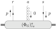
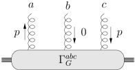
Figure 2: We encounter three different types of gluonic pole matrix elements (GPME’s): the quark-GPME $\Phi_{G}{=}(\Phi_{G})_{rs}^{a}(t^{a})_{sr}{=}\operatorname{Tr}[\Phi_{G}^{a}t^{a}]$ and the two gluon-GPME’s $\Gamma_{G}^{(f)}{=}\Gamma_{G}^{abc}(t^{a})_{cb}{=}\Gamma_{G}^{abc}if^{abc}$ and $\Gamma_{G}^{(d)}{=}\Gamma_{G}^{abc}d^{abc}$. The $d^{abc}$ and $f^{abc}$ are the symmetric and antisymmetric structure constants of $SU(3)$: $t^{a}t^{b}{=}\frac{T_{F}}{N}\delta^{ab}{+}\frac{1}{2}\left(d^{abc}{+}if^{abc}\right)t^{c}$.

The treatment of antiquark distribution and fragmentation follows along similar lines as described above. The results are summarized in appendix A. Gluon distribution correlators are written as the product of two gluon field-strength tensors and two gauge-links connecting them, see (36). The product of operators is in the 3-dimensional fundamental representation of the color matrices and appears traced in the correlators. Due to the presence of two gauge-links (in the matrix representation), rather than one, as was the case in quark distribution, there are two different types of gluonic pole matrix elements: those with soft gluons arising from the gauge-link $\mathcal{U}$ or $\mathcal{U}^{\prime}$, respectively. This complicates the occurrence of $T$-odd effects in gluon distributions somewhat. Since the correlator is color-traced, it is convenient to consider the commutator and anticommutator combinations of gluon fields in the matrix elements. These involve the symmetric and the antisymmetric structure constants of $SU(3)$ color (Figure 2). Taking the first moment of the gluon correlator (36a) it follows that

$$\Gamma^{[\mathcal{U}\mathcal{U}^{\prime}]\alpha}_{\partial}(x)=\widetilde{\Gamma}_{\partial}^{\alpha}(x)+C_{G}^{(f)}\,\pi\Gamma_{G}^{(f)}{}^{\alpha}(x,x)+C_{G}^{(d)}\,\pi\Gamma_{G}^{(d)}{}^{\alpha}(x,x)\ ,$$ (12)

where the gluonic pole strengths $C_{G}^{(f/d)}$ involve sums and differences of contributions arising from the two different gauge-links. The matrix element $\widetilde{\Gamma}_{\partial}$ (which is purely $T$-even in the case of gluon distribution) only involves a color commutator (cf. (41e) and (39f)). The definitions of the different matrix elements appearing in this expression are given in appendix A. The leading contributions to the collinear gluon correlator is parametrized as follows

$$2x\,\Gamma^{ij}(x)=-g_{T}^{ij}\,G(x)-S_{L}\,i\epsilon_{T}^{ij}\,\Delta G(x)\ .\\$$ (13)

For the gluon fragmentation correlator we use a similar parametrization. It is obtained by making the substitutions $\big{\{}2x\Gamma(x),G(x),\Delta G(x)\big{\}}{\rightarrow}\big{\{}\widehat{\Gamma}(\frac{1}{z}),\widehat{G}(z),\Delta\widehat{G}(z)\big{\}}$. Following the treatment of TMD functions in Ref. Mulders and Rodrigues (2001) we take for the $\widetilde{\Gamma}_{\partial}(x)$ and the gluonic pole matrix elements the parametrizations

$$2x\,\widetilde{\Gamma}^{ij;\alpha}(x)=-M\,i\epsilon_{T}^{ij}S_{T}^{\alpha}\,\Delta G_{T}^{(1)}(x)\ ,$$ (14a)

$$2x\,\pi\Gamma_{G}^{(f/d)}{}^{ij;\alpha}(x,x)=M\,g_{T}^{ij}\epsilon_{T}^{S_{T}\alpha}\,G_{T}^{(f/d)}{}^{(1)}(x)-\tfrac{1}{2}M\,\big{(}\epsilon_{T}^{\alpha\{i}S_{T}^{j\}}{+}\epsilon_{T}^{S_{T}\{i}g_{T}^{j\}\alpha}\big{)}\,\Delta H_{T}^{(f/d)}{}^{(1)}(x)\ .$$ (14b)

The indices $i$, $j$ and $\alpha$ are all transverse w.r.t. the hadron direction and its conjugate direction (cf. (1)). The functions $\Delta H_{T}^{(1)}$ involve a flip of gluon helicity in a transversally polarized target. The functions $G_{T}^{(1)}$ and $\Delta G_{T}^{(1)}$ do not flip the gluons helicity and represent unpolarized and polarized gluons in transversally polarized targets, respectively. Note that the $T$-odd quark and gluon distribution (fragmentation) functions that appear in the parametrizations of the gluonic pole matrix elements are different from quark-quark or gluon-gluon matrix elements. They contain an additional zero-momentum gluon (the gluonic pole). Therefore, it is not obvious if such $T$-odd functions can be interpreted as probability distributions. The emergence of two (the $f$ and the $d$) $T$-odd gluon distribution (or fragmentation) functions is simply the consequence of the two possible orderings of the three gluons in the matrix element $\Gamma_{G}$ in figure 2.

From symmetry relations it follows that $G_{T}^{(f/d)}{}^{(1)}(x)$ can be written as the $x$-even and $x$-odd combinations of a single gluon distribution function, i.e. $G_{T}^{(f/d)}{}^{(1)}(x){=}\frac{1}{2}\big{(}G_{T}^{(1)}(x){\pm}G_{T}^{(1)}({-}x)\big{)}$ and similarly for $\Delta H_{T}^{(f/d)}{}^{(1)}(x)$. As seen in equation (12) the $x$-even and $x$-odd combinations of gluon distribution functions can appear with different prefactors. Hence, the description of the gluon contribution to $T$-odd effects involves two different gluonic pole cross sections, one containing the gluonic pole factors $C_{G}^{(d)}$ and one containing the factors $C_{G}^{(f)}$. Using the results of Bomhof et al. (2006) we can give all gluonic pole strengths $C_{G}$ appearing in $2{\rightarrow}2$ scattering processes with external gluons. They are listed in Tables 4-8. The treatment of gluon fragmentation is the obvious extension of the formalism described above.

The gluonic pole strengths associated with quarks $C_{G}(q)$ calculated in the way described above are related to the color factors calculated by Qiu and Sterman in Ref. Qiu and Sterman (1999), who consider one-pion inclusive proton-proton scattering $pp{\rightarrow}\pi X$. The relation is Vogelsang

$$C_{G}(q)=\frac{C_{q/g}^{I}{+}C_{q/g}^{F}{+}C_{q/g}^{F^{\prime}}}{C_{q/g}}\ ,$$ (15)

where $C_{q/g}$, $C_{q/g}^{I}$ and $C_{q/g}^{F}$ are the color factors defined and calculated in Ref. Qiu and Sterman (1999) (one should note that some of the color factors in Table II of that reference are erroneous). The factor $C_{q/g}$ is the color factor of the spin-averaged subprocess. The factor $C_{q/g}^{I}$ is the color factor of the spin-dependent subprocess with a gluon attachment on the (other) incoming parton and the factor $C_{q/g}^{F}$ is the color factor of the spin-dependent subprocess with a gluon attachment on the outgoing parton that fragments into the observed pion. The factor $C_{q/g}^{F^{\prime}}$ is the corresponding color factor of the spin-dependent subprocess with a gluon attachment on the other outgoing parton. These factors have not been given in Ref. Qiu and Sterman (1999), where it is argued that they are not needed in the one-pion inclusive process. They can be calculated in exactly the same way as the factors $C^{I}$ and $C^{F}$. They can also be obtained from symmetry considerations. The color factor $C^{F^{\prime}}$ of the process $ab{\rightarrow}c_{\pi}d$ should be the same as the color factor $C^{F}$ of the process $ab{\rightarrow}cd_{\pi}$ (the subscript $\pi$ indicating which parton fragments into the observed pion).

(a)

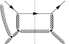
(b)

(c)

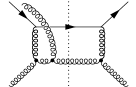
(d)

Figure 3: A contribution to $qg{\rightarrow}qg$ scattering (a) and some collinear gluon insertions (b)-(d).

As an example we consider the contribution of the diagram in Figure 3a to quark-gluon scattering $qg{\rightarrow}qg$ explicitly. In this example the quark comes from the polarized hadron and it is also the quark that fragments into the observed pion. In that case Figures 3a, 3b and 3c correspond to the Figures 15a, 16a and 16b of Ref. Qiu and Sterman (1999). From the first line of Table I in Qiu and Sterman (1999) one finds their color factors: $C_{g}{=}\frac{1}{2}$, $C_{g}^{I}{=}{-}N^{2}/4(N^{2}{-}1)$ and $C_{g}^{F}{=}{-}1/2(N^{2}{-}1)$. The color factor corresponding to the gluon insertion in Figure 3d is calculated to be $C_{g}^{F^{\prime}}{=}N^{2}/4(N^{2}{-}1)$. Hence, the relation in Eq. (15) indeed reproduces the gluonic pole strength $C_{G}(q){=}{-}1/(N^{2}{-}1)$. The color factor $C_{g}^{F^{\prime}}$ that we have just calculated would have been the same as the color factor $C_{g}^{F}$ of the corresponding contribution to $qg{\rightarrow}qg_{\pi}$ scattering if Ref. Qiu and Sterman (1999) would have considered the possibility that it is the gluon that fragments into the observed pion.

IV Gluonic Pole Scattering Cross Sections

As indicated in previous sections we aim at a description of single spin asymmetries as convolutions of universal collinear parton distribution and fragmentation functions and perturbatively calculable hard parts. These convolutions involve an odd number of (usually one) $T$-odd distribution or fragmentation functions. The basic observation of the previous section is that the gluonic pole matrix elements that contain the $T$-odd functions are multiplied by gluonic pole factors $C_{G}$. These might be different for each Feynman diagram $D$ that contributes to the partonic scattering process. Consequently, the hard part in the description of the SSA, in general, no longer equals the basic partonic scattering cross section in Eq. (6), but rather the gluonic pole cross sections in Eq. (7). For instance, in the identical quark scattering contribution to $p^{\uparrow}p{\rightarrow}\pi\pi X$ (see next section) the direct scattering channels (first and second diagram in Table 4) get the factor $C_{G}{=}(N^{2}{-}5)/(N^{2}{-}1){=}\frac{1}{2}$ and the interference terms (third and fourth diagram in Table 4) get the factor $C_{G}{=}{-}(N^{2}{+}3)/(N^{2}{-}1){=}{-}\frac{3}{2}$ from the incoming quark. Accordingly, the Sivers effect for the identical quark scattering contribution to $p^{\uparrow}p{\rightarrow}\pi\pi X$ appears proportional to

$$f_{1T}^{\perp(1)}(x_{1})\,f_{1}(x_{2})\,\bigg{(}\{\tfrac{1}{2}\}\parbox{42.67912pt}{\includegraphics[width=42.67912pt]{Figures/qq2qqA.eps}}+\{\tfrac{1}{2}\}\parbox{42.67912pt}{\includegraphics[width=42.67912pt]{Figures/qq2qqB.eps}}-\{{-}\tfrac{3}{2}\}\parbox{42.67912pt}{\includegraphics[width=42.67912pt]{Figures/qq2qqC.eps}}-\{{-}\tfrac{3}{2}\}\parbox{42.67912pt}{\includegraphics[width=42.67912pt]{Figures/qq2qqD.eps}}\,\bigg{)}\,D_{1}(z_{1})\,D_{1}(z_{2})\ ,$$ (16)

(compare this with the situation in SIDIS and DY, cf. Eq. (5)). Therefore, as a consequence of the gauge-links the contribution of the Sivers effect is a convolution of the Sivers function with the unpolarized distribution and fragmentation functions and the hard cross section

$$\frac{d\hat{\sigma}_{[q]q{\rightarrow}qq}}{d\hat{t}}=\tfrac{1}{2}\parbox{42.67912pt}{\includegraphics[width=42.67912pt]{Figures/qq2qqA.eps}}+\tfrac{1}{2}\parbox{42.67912pt}{\includegraphics[width=42.67912pt]{Figures/qq2qqB.eps}}+\tfrac{3}{2}\parbox{42.67912pt}{\includegraphics[width=42.67912pt]{Figures/qq2qqC.eps}}+\tfrac{3}{2}\parbox{42.67912pt}{\includegraphics[width=42.67912pt]{Figures/qq2qqD.eps}}\,=\frac{4\pi\alpha_{S}^{2}}{9\hat{s}^{2}}\,\bigg{\{}\,\frac{\hat{s}^{2}{+}\hat{u}^{2}}{2\hat{t}^{2}}+\frac{\hat{s}^{2}{+}\hat{t}^{2}}{2\hat{u}^{2}}+\frac{\hat{s}^{2}}{\hat{t}\hat{u}}\,\bigg{\}}\ .$$ (17)

We refer to this as a gluonic pole scattering cross section and it should be contrasted to the standard partonic cross section

$$\frac{d\hat{\sigma}_{qq{\rightarrow}qq}}{d\hat{t}}=\parbox{42.67912pt}{\includegraphics[width=42.67912pt]{Figures/qq2qqA.eps}}+\parbox{42.67912pt}{\includegraphics[width=42.67912pt]{Figures/qq2qqB.eps}}-\parbox{42.67912pt}{\includegraphics[width=42.67912pt]{Figures/qq2qqC.eps}}-\parbox{42.67912pt}{\includegraphics[width=42.67912pt]{Figures/qq2qqD.eps}}\,=\frac{4\pi\alpha_{S}^{2}}{9\hat{s}^{2}}\,\bigg{\{}\,\frac{\hat{s}^{2}{+}\hat{u}^{2}}{\hat{t}^{2}}+\frac{\hat{s}^{2}{+}\hat{t}^{2}}{\hat{u}^{2}}-\frac{2}{3}\frac{\hat{s}^{2}}{\hat{t}\hat{u}}\,\bigg{\}}\ ,$$ (18)

(see Figure 4).

For quark fragmentation the situation is more involved. As mentioned, due to the internal final state interactions both terms on the r.h.s. of expression (11) can contribute to the $T$-odd effects. The matrix element $\widetilde{\Delta}_{\partial}\big{(}\tfrac{1}{z}\big{)}$ appears in the same way, regardless of the process, while the gluonic pole matrix element occurs multiplied by the gluonic pole factors $C_{G}$, which depend on the gauge-links and, hence, on the hard subprocess. Comparing this with the case of quark distribution described above, we see that the non-tilde-functions appear with the standard partonic cross sections and the tilde-functions appear with gluonic pole cross sections. For instance, for the identical quark subprocess in $p^{\uparrow}p{\rightarrow}\pi\pi X$ scattering the gluonic pole factors associated with the fragmenting quark are $C_{G}{=}{-}\frac{1}{2}$ for the direct scattering channels and $C_{G}{=}\frac{3}{2}$ for the interference terms. Therefore, the Collins effect becomes

$$h_{1}(x_{1})\,f_{1}(x_{2})\,\frac{d\Delta\hat{\sigma}_{q^{\uparrow}q{\rightarrow}q^{\uparrow}q}}{d\hat{t}}\,H_{1}^{\perp(1)}(z_{1})\,D_{1}(z_{2})+h_{1}(x_{1})\,f_{1}(x_{2})\,\frac{d\Delta\hat{\sigma}_{q^{\uparrow}q{\rightarrow}[q^{\uparrow}]q}}{d\hat{t}}\,\widetilde{H}{}_{1}^{\perp(1)}(z_{1})\,D_{1}(z_{2})\ ,$$ (19)

where $h_{1}$ is the transversity distribution function. The $d\Delta\hat{\sigma}_{q^{\uparrow}q{\rightarrow}q^{\uparrow}q}/d\hat{t}$ is the standard partonic cross section and $d\Delta\hat{\sigma}_{q^{\uparrow}q{\rightarrow}[q^{\uparrow}]q}/d\hat{t}$ is the gluonic pole cross section

$$\frac{d\Delta\hat{\sigma}_{q^{\uparrow}q{\rightarrow}q^{\uparrow}q}}{d\hat{t}}=\parbox{42.67912pt}{\includegraphics[width=42.67912pt]{Figures/qq2qqA.eps}}+\parbox{42.67912pt}{\includegraphics[width=42.67912pt]{Figures/qq2qqB.eps}}-\parbox{42.67912pt}{\includegraphics[width=42.67912pt]{Figures/qq2qqC.eps}}-\parbox{42.67912pt}{\includegraphics[width=42.67912pt]{Figures/qq2qqD.eps}}\ ,$$ (20a)

$$\frac{d\Delta\hat{\sigma}_{q^{\uparrow}q{\rightarrow}[q^{\uparrow}]q}}{d\hat{t}}=-\tfrac{1}{2}\parbox{42.67912pt}{\includegraphics[width=42.67912pt]{Figures/qq2qqA.eps}}-\tfrac{1}{2}\parbox{42.67912pt}{\includegraphics[width=42.67912pt]{Figures/qq2qqB.eps}}-\tfrac{3}{2}\parbox{42.67912pt}{\includegraphics[width=42.67912pt]{Figures/qq2qqC.eps}}-\tfrac{3}{2}\parbox{42.67912pt}{\includegraphics[width=42.67912pt]{Figures/qq2qqD.eps}}\ .$$ (20b)

At this point we would like to recall once more that the case of universality of quark fragmentation as conjectured in Ref. Collins and Metz (2004) is included as the situation of vanishing tilde-fragmentation functions. There would, then, be no gluonic pole scattering cross sections associated with quark fragmentation. Some gluonic pole cross sections associated with quarks are given in the Tables 8, 10 and 13. The others can be obtained from these by using the symmetries described at the end of this section. For comparison we also give the partonic cross sections, Tables 8, 10 and 13 (all cross sections are given for massless quarks). The gluonic pole cross sections for fermionic scattering have already been calculated in Bacchetta et al. (2005) and have been reproduced in the tables for completeness. Using the gluonic pole strengths calculated in the previous section we can now also give the gluonic pole cross sections for processes with external gluons. These expressions are important since at high energies gluon scattering is expected to be the dominant channel Boer and Vogelsang (2004); Anselmino et al. (2006).

The leading contribution to the parametrization of the gluon correlators (36) are transverse to both the momentum of the parent/daughter hadron and its conjugate direction. The constraint on this conjugate $n$-direction is that it has a nonvanishing overlap with the hadron’s momentum, but can otherwise be chosen arbitrarily. The expressions for the individual diagrams are not independent of these $n$-vectors. They enter the expression through the parametrization of the gluon correlators (13) and, for each external gluon, there can be a different $n$-vector. However, in the basic partonic cross sections in Eq. (6) as well as in the gluonic pole cross sections in Eqs. (7) all the $n$-dependencies cancel.

To illustrate the role of gluons we take quark-gluon scattering as an example. If in unpolarized scattering the incoming quark contributes the gluonic pole, then the corresponding expression in the hadronic scattering cross section will involve the gluonic pole cross section $d\hat{\sigma}_{[q]g\rightarrow qg}/d\hat{t}$ given in Table 8. It is obtained by summing the expressions for the diagrams in the first column of Table 8 after multiplying them with the factors $C_{G}(q_{i})$ in the second column. In this summation, as with all other gluonic pole cross sections, all $n$-dependencies cancel. The situation becomes more complicated when it is the incoming gluon that contributes the gluonic pole. From equation (12) and using the results in the third and fourth columns of Table 8 we see that the gluon-Sivers contribution to the cross section has the form

$$G_{T}^{(f)}{}^{(1)}(x_{1})f_{1}(x_{2})\,\frac{d\hat{\sigma}_{[g]q\rightarrow gq}^{(f)}}{d\hat{t}}\,\widehat{G}(z_{1})D_{1}(z_{2})+G_{T}^{(d)}{}^{(1)}(x_{1})f_{1}(x_{2})\,\frac{d\hat{\sigma}_{[g]q\rightarrow gq}^{(d)}}{d\hat{t}}\,\widehat{G}(z_{1})D_{1}(z_{2})\ .$$ (21)

Hence, the two possible $T$-odd gluon distribution functions (the $x$-even and $x$-odd combinations) multiply two distinct gluonic pole cross sections, one containing the weight factors $C_{G}^{(f)}$ and one containing the weights $C_{G}^{(d)}$. All the gluonic pole cross sections associated with a gluon are given in the tables 13-15.

In Table 8 only the diagrams without 4-gluon vertices have been given. When 4-gluon vertices are involved, things become slightly more subtle. At the heart of the problem is that the color structure of the 4-gluon vertex does not factorize from the kinematical part. This is, then, also the case for the diagram containing the 4-gluon vertex. This observation has important consequences for the summation of all collinear gluon interactions between the hard and soft parts, which leads to the gauge-links in the parton correlators. As an example we consider the diagram

$$\parbox{42.67912pt}{ \includegraphics[width=42.67912pt]{Figures/gg2ggH.eps}}=K_{1}\times\left\{\,\parbox{42.67912pt}{ \includegraphics[width=42.67912pt]{Figures/gg2ggA.eps}}\,\right\}_{c}+K_{2}\times\left\{\,\parbox{42.67912pt}{ \includegraphics[width=42.67912pt]{Figures/gg2ggN.eps}}\,\right\}_{c}+K_{3}\times\left\{\,\parbox{42.67912pt}{ \includegraphics[width=42.67912pt]{Figures/gg2ggE.eps}}\,\right\}_{c}\ .$$ (22)

On the r.h.s. we have made a color-decomposition by inserting the expression of the 4-gluon vertex. The $K_{i}$ contain all the kinematical parts and the bracketed diagrams $\{D\}_{c}$ refer to the color structure of that diagram. Ultimately, it is the color structure that fixes the gauge-link Bomhof et al. (2006). Hence, the three terms on the r.h.s. of (22) are convoluted with the gauge-invariant correlators of the corresponding color-diagrams (these are given in Table 8 of Ref. Bomhof et al. (2006)). Accordingly, when weighing, the three terms get multiplied by the gluonic pole strengths of the corresponding color-diagrams. That is, the first term on the r.h.s. of (22) gets multiplied by the gluonic pole factors in the second row of Table 8, the second term gets multiplied by the factors in the last row and the third term gets multiplied by the factors in the fifth row. As a result, the expression of our diagram as it appears in the calculation of the gluonic pole cross section $d\hat{\sigma}_{[g]g\rightarrow gg}^{(f)}$ is

$$\parbox{42.67912pt}{ \includegraphics[width=42.67912pt]{Figures/gg2ggH.eps}}\longrightarrow\tfrac{1}{2}\times K_{1}\times\left\{\,\parbox{42.67912pt}{ \includegraphics[width=42.67912pt]{Figures/gg2ggA.eps}}\,\right\}_{c}+1\times K_{2}\times\left\{\,\parbox{42.67912pt}{ \includegraphics[width=42.67912pt]{Figures/gg2ggN.eps}}\,\right\}_{c}+0\times K_{3}\times\left\{\,\parbox{42.67912pt}{ \includegraphics[width=42.67912pt]{Figures/gg2ggE.eps}}\,\right\}_{c}\ .$$ (23)

Therefore, the summation in (7) is seen to actually run over the color-decomposed diagrams. The expressions for the other diagrams with 4-gluon vertices can be calculated in much the same way and the results are summarized in the tables 13-15.

$d\hat{\sigma}_{[q]q\rightarrow qq}/d\hat{\sigma}_{qq\rightarrow qq}$

$d\hat{\sigma}_{[q]\bar{q}\rightarrow q\bar{q}}/d\hat{\sigma}_{q\bar{q}\rightarrow q\bar{q}}$

$d\hat{\sigma}_{[q]g\rightarrow qg}/d\hat{\sigma}_{qg\rightarrow qg}$

$d\hat{\sigma}_{[q]\bar{q}\rightarrow gg}/d\hat{\sigma}_{q\bar{q}\rightarrow gg}$

Figure 4: Ratios of gluonic pole cross sections and partonic cross sections for some gluonic pole cross sections associated with quarks. They are plotted as functions of the variable $y{\equiv}{-}\hat{t}/\hat{s}$ for $N{=}3$ (solid line) and $N{\rightarrow}\infty$ (dashed line).

We will end this section by making some observations about the properties of the gluonic pole cross sections. First of all, the different gluonic pole cross sections cannot be related to one another using the crossing symmetries that exist among the partonic cross sections. A simple example is $ud{\rightarrow}ud$ versus $u\bar{u}{\rightarrow}d\bar{d}$ scattering. The first process is described by a $t$-channel diagram and the second by an $s$-channel diagram. Correspondingly, the partonic cross sections can be related by replacing the Mandelstam variables $\hat{s}$ and $\hat{t}$ (cf. Table 8). Going to the gluonic pole cross sections these two diagrams are multiplied by different gluonic pole factors. Hence, the gluonic pole cross sections are not related by an $\hat{s}{\leftrightarrow}\hat{t}$ crossing (even simpler are the processes $ud{\rightarrow}ud$ and $u\bar{d}{\rightarrow}u\bar{d}$ that have the same partonic cross sections, but different gluonic pole cross sections). The only crossing symmetry that survives in the gluonic pole cross sections is the substitution $\hat{t}{\leftrightarrow}\hat{u}$ when interchanging two partons in the initial or final state. For a particular partonic process, there are some relations between the gluonic pole cross sections with the gluonic pole associated with different partons. Using the relations between gluonic pole factors described in the tables in the previous section, it is seen that

$$\frac{d\hat{\sigma}_{[q_{1}]q_{2}\rightarrow ab}}{d\hat{t}} =\frac{d\hat{\sigma}_{q_{1}[q_{2}]\rightarrow ab}}{d\hat{t}}\ , \qquad\frac{d\hat{\sigma}_{ab\rightarrow[q_{1}]q_{2}}}{d\hat{t}} =\frac{d\hat{\sigma}_{ab\rightarrow q_{1}[q_{2}]}}{d\hat{t}}\ , \qquad\frac{d\hat{\sigma}_{[q_{1}]a\rightarrow q_{2}b}}{d\hat{t}} =-\frac{d\hat{\sigma}_{q_{1}a\rightarrow[q_{2}]b}}{d\hat{t}}\ ,$$ (24a)

where $$q_{1} q_{2}$$ and can be any quark or antiquark. For the gluonic pole cross sections where the gluonic pole is associated with a gluon we have the following relations

$$\frac{d\hat{\sigma}_{[g]g\rightarrow ab}^{(d)}}{d\hat{t}} =-\frac{d\hat{\sigma}_{g[g]\rightarrow ab}^{(d)}}{d\hat{t}}\ , \frac{d\hat{\sigma}_{ab\rightarrow[g]g}^{(d)}}{d\hat{t}} =-\frac{d\hat{\sigma}_{ab\rightarrow g[g]}^{(d)}}{d\hat{t}}\ , \frac{d\hat{\sigma}_{[g]a\rightarrow gb}^{(d)}}{d\hat{t}} =\phantom{-}\frac{d\hat{\sigma}_{ga\rightarrow[g]b}^{(d)}}{d\hat{t}}\ ,$$ (24b)

$$\frac{d\hat{\sigma}_{[g]g\rightarrow ab}^{(f)}}{d\hat{t}} =\phantom{-}\frac{d\hat{\sigma}_{g[g]\rightarrow ab}^{(f)}}{d\hat{t}}\ , \frac{d\hat{\sigma}_{ab\rightarrow[g]g}^{(f)}}{d\hat{t}} =\phantom{-}\frac{d\hat{\sigma}_{ab\rightarrow g[g]}^{(f)}}{d\hat{t}}\ , \frac{d\hat{\sigma}_{[g]a\rightarrow gb}^{(f)}}{d\hat{t}} =-\frac{d\hat{\sigma}_{ga\rightarrow[g]b}^{(f)}}{d\hat{t}}\ .$$ (24c)

In (24) the $a$ and $b$ can be any colored parton (quark, antiquark or gluon). These symmetries also hold for the polarized cross sections.

Just as for the gluonic pole factors in Eq. (15) there is a relation Vogelsang between the gluonic pole scattering cross sections associated with quarks as calculated in this section and the hard parts $H^{I/F}$ calculated in Qiu and Sterman (1999); Kouvaris et al. (2006):

$$\frac{d\hat{\sigma}_{[q]b\rightarrow cd}}{d\hat{t}}=H^{I}_{qb\rightarrow c}+H^{F}_{qb\rightarrow c}+H^{F^{\prime}}_{qb\rightarrow c}\ .$$ (25)

The $H^{F^{\prime}}$ for the process $ab{\rightarrow}c_{\pi}d$ is the same as the $H^{F}$ of the process $ab{\rightarrow}cd_{\pi}$ which, in turn, can be related to the $H^{F}$ of the process $ab{\rightarrow}d_{\pi}c$ by a $\hat{t}{\leftrightarrow}\hat{u}$ interchange.

V Gluonic pole cross sections in $p^{\uparrow}p{\rightarrow}\pi\pi X$.

As an illustration of the appearance of gluonic pole cross sections in physical processes we consider inclusive back-to-back pion production in proton-proton scattering $p^{\uparrow}p{\rightarrow}\pi\pi X$, Figure 5. In this process, they appear as leading contributions in the azimuthal asymmetry considered below. Using the decompositions (1) $p^{\uparrow}p{\rightarrow}\pi\pi X$ is given in terms of parton correlators by

$$\langle d\sigma_{h_{1}h_{2}}\rangle=\int d\phi_{2}\,\frac{d\sigma_{h_{1}h_{2}}}{d\phi_{2}}=\frac{dx_{1\perp}dx_{2\perp}d\eta_{1}d\eta_{2}}{32\pi s}\frac{d\phi_{1}}{2\pi}\int\frac{dx_{\perp}}{x_{\perp}}\ \Sigma(x_{1},x_{2},z_{1},z_{2},y)\ ,$$ (26a)

where the momentum fractions are given in terms of the kinematical variables as in Ref. Bacchetta et al. (2005). In that reference it was found that the azimuthal asymmetry

$$\langle\tfrac{1}{2}\sin(\delta\phi)\,d\sigma_{h_{1}h_{2}}\rangle=\int d\phi_{2}\,\tfrac{1}{2}\sin(\delta\phi)\,\frac{d\sigma_{h_{1}h_{2}}}{d\phi_{2}}=\frac{dx_{1\perp}dx_{2\perp}d\eta_{1}d\eta_{2}}{32\pi s\sqrt{s}}\frac{d\phi_{1}}{2\pi}\int\frac{dx_{\perp}}{x_{\perp}^{2}}\ e_{1N}{\cdot}\Sigma_{\partial}(x_{1},x_{2},z_{1},z_{2},y)\ ,$$ (26b)

contains the leading twist $T$-odd effects. In these expressions we have used the quantities

$$\Sigma(x_{1},x_{2},z_{1},z_{2},y) =\sum\operatorname{Tr}\big{\{}\,\Phi(x_{1})\Phi(x_{2})\Delta(z_{1})\Delta(z_{2})\,H\,H^{*}\,\big{\}}\ ,$$ (27)

$$\Sigma_{\partial}^{\alpha}(x_{1},x_{2},z_{1},z_{2},y) =\sum\operatorname{Tr}\big{\{}\,\big{[}\Phi_{\partial}^{\alpha}(x_{1})\Phi(x_{2})\Delta(z_{1})\Delta(z_{2}){+}\Phi(x_{1})\Phi_{\partial}^{\alpha}(x_{2})\Delta(z_{1})\Delta(z_{2})$$

$$\mspace{100.0mu}{-}\Phi(x_{1})\Phi(x_{2})\Delta_{\partial}^{\alpha}(z_{1})\Delta(z_{2}){-}\Phi(x_{1})\Phi(x_{2})\Delta(z_{1})\Delta_{\partial}^{\alpha}(z_{2})\big{]}\,H\,H^{*}\,\big{\}}$$ (28)

$$\equiv\Sigma_{1\,\partial}^{\alpha}+\Sigma_{2\,\partial}^{\alpha}-\Sigma_{1^{\prime}\,\partial}^{\alpha}-\Sigma_{2^{\prime}\,\partial}^{\alpha}\ .$$ (29)

The quantity $H{=}H(x_{1},x_{2},z_{1},z_{2})$ is the collinear hard part and the summation runs over all parton correlators as given in appendix A.

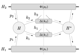
Figure 5: The leading order contribution to the cross section of $H_{1}{+}H_{2}\rightarrow h_{1}{+}h_{2}{+}X$.

For the parametrizations of the different correlators we use the conventions of Ref. Bacchetta et al. (2005) and Eqs. (13) and (14). Inserting these parametrizations in the expressions for the cross sections, one obtains

$$\frac{\Sigma(x_{1},x_{2},z_{1},z_{2},y)}{32\pi s}$$

$$\mspace{50.0mu}=\sum_{\begin{subarray}{c}\text{(anti)quark}\\ \text{flavors}\end{subarray}}\Big{\{}\,f_{1}(x_{1})f_{1}(x_{2})\,\frac{\hat{s}}{2}\frac{d\hat{\sigma}_{q_{1}q_{2}\rightarrow q_{3}q_{4}}}{d\hat{t}}\,D_{1}(z_{1})D_{1}(z_{2})$$ (30a)

$$\mspace{190.0mu}+f_{1}(x_{1})G(x_{2})\,\frac{\hat{s}}{2}\frac{d\hat{\sigma}_{qg\rightarrow qg}}{d\hat{t}}\,D_{1}(z_{1})\widehat{G}(z_{2})\ +\big{(}K_{1}{\leftrightarrow}K_{2}\big{)}$$ (30b)

$$\mspace{190.0mu}+G(x_{1})f_{1}(x_{2})\,\frac{\hat{s}}{2}\frac{d\hat{\sigma}_{gq\rightarrow gq}}{d\hat{t}}\,\widehat{G}(z_{1})D_{1}(z_{2})\ +\big{(}K_{1}{\leftrightarrow}K_{2}\big{)}$$ (30c)

$$\mspace{190.0mu}+f_{1}(x_{1})\bar{f}_{1}(x_{2})\,\frac{\hat{s}}{2}\frac{d\hat{\sigma}_{q\bar{q}\rightarrow gg}}{d\hat{t}}\,\widehat{G}(z_{1})\widehat{G}(z_{2})$$ (30d)

$$\mspace{190.0mu}+G(x_{1})G(x_{2})\,\frac{\hat{s}}{2}\frac{d\hat{\sigma}_{gg\rightarrow q\bar{q}}}{d\hat{t}}\,D_{1}(z_{1})\bar{D}_{1}(z_{2})$$ (30e)

$$\mspace{190.0mu}+G(x_{1})G(x_{2})\,\frac{\hat{s}}{2}\frac{d\hat{\sigma}_{gg\rightarrow gg}}{d\hat{t}}\,\widehat{G}(z_{1})\widehat{G}(z_{2})\ \Big{\}}\ ,$$ (30f)

where the summation runs over all quarks and antiquarks (we have suppressed the parton indices on the distribution and fragmentation functions). For the polarized cross section we get (the quark-scattering contributions were already obtained in Eqs. (30)-(32) and (D1)-(D3) of Ref. Bacchetta et al. (2005), but with a wrong overall sign)

$$-\frac{e_{1N}\cdot\Sigma_{1\,\partial}(x_{1},x_{2},z_{1},z_{2},y)}{32\pi s\,M_{1}\cos(\phi_{1}{-}\phi_{S})}$$

$$\mspace{50.0mu}=\sum_{\begin{subarray}{c}\text{(anti)quark}\\ \text{flavors}\end{subarray}}\bigg{\{}\ f_{1T}^{\perp(1)}(x_{1})f_{1}(x_{2})\,\frac{\hat{s}}{2}\frac{d\hat{\sigma}_{[q_{1}]q_{2}\rightarrow q_{3}q_{4}}}{d\hat{t}}\,D_{1}(z_{1})D_{1}(z_{2})$$ (31a)

$$\mspace{190.0mu}+f_{1T}^{\perp(1)}(x_{1})G(x_{2})\,\frac{\hat{s}}{2}\frac{d\hat{\sigma}_{[q]g\rightarrow qg}}{d\hat{t}}\,D_{1}(z_{1})\widehat{G}(z_{2})\ +\big{(}K_{1}{\leftrightarrow}K_{2}\big{)}$$ (31b)

$$\mspace{190.0mu}+f_{1T}^{\perp(1)}(x_{1})\bar{f}_{1}(x_{2})\,\frac{\hat{s}}{2}\frac{d\hat{\sigma}_{[q]\bar{q}\rightarrow gg}}{d\hat{t}}\,\widehat{G}(z_{1})\widehat{G}(z_{2})$$ (31c)

$$\mspace{190.0mu}+G_{T}^{(d)}{}^{(1)}(x_{1})f_{1}(x_{2})\,\frac{\hat{s}}{2}\frac{d\hat{\sigma}_{[g]q\rightarrow gq}^{(d)}}{d\hat{t}}\,\widehat{G}(z_{1})D_{1}(z_{2})\ +\big{(}K_{1}{\leftrightarrow}K_{2}\big{)}$$ (31d)

$$\mspace{190.0mu}+G_{T}^{(f)}{}^{(1)}(x_{1})f_{1}(x_{2})\,\frac{\hat{s}}{2}\frac{d\hat{\sigma}_{[g]q\rightarrow gq}^{(f)}}{d\hat{t}}\,\widehat{G}(z_{1})D_{1}(z_{2})\ +\big{(}K_{1}{\leftrightarrow}K_{2}\big{)}$$ (31e)

$$\mspace{190.0mu}+G_{T}^{(d)}{}^{(1)}(x_{1})G(x_{2})\,\frac{\hat{s}}{2}\frac{d\hat{\sigma}_{[g]g\rightarrow q\bar{q}}^{(d)}}{d\hat{t}}\,D_{1}(z_{1})\bar{D}_{1}(z_{2})$$ (31f)

$$\mspace{190.0mu}+G_{T}^{(f)}{}^{(1)}(x_{1})G(x_{2})\,\frac{\hat{s}}{2}\frac{d\hat{\sigma}_{[g]g\rightarrow q\bar{q}}^{(f)}}{d\hat{t}}\,D_{1}(z_{1})\bar{D}_{1}(z_{2})$$ (31g)

$$\mspace{190.0mu}+G_{T}^{(d)}{}^{(1)}(x_{1})G(x_{2})\,\frac{\hat{s}}{2}\frac{d\hat{\sigma}_{[g]g\rightarrow gg}^{(d)}}{d\hat{t}}\,\widehat{G}(z_{1})\widehat{G}(z_{2})$$ (31h)

$$\mspace{190.0mu}+G_{T}^{(f)}{}^{(1)}(x_{1})G(x_{2})\,\frac{\hat{s}}{2}\frac{d\hat{\sigma}_{[g]g\rightarrow gg}^{(f)}}{d\hat{t}}\,\widehat{G}(z_{1})\widehat{G}(z_{2})\ \Big{\}}\ ,$$ (31i)

$$-\frac{e_{1N}\cdot\Sigma_{2\,\partial}(x_{1},x_{2},z_{1},z_{2},y)}{32\pi s\,M_{2}\cos(\phi_{1}{-}\phi_{S})}$$

$$\mspace{50.0mu}=\sum_{\begin{subarray}{c}\text{(anti)quark}\\ \text{flavors}\end{subarray}}\bigg{\{}\ h_{1}(x_{1})h_{1}^{\perp(1)}(x_{2})\,\frac{\hat{s}}{2}\frac{d\Delta\hat{\sigma}_{q_{1}^{\uparrow}[q_{2}^{\uparrow}]\rightarrow q_{3}q_{4}}}{d\hat{t}}\,D_{1}(z_{1})D_{1}(z_{2})$$ (32a)

$$\mspace{190.0mu}+h_{1}(x_{1})\bar{h}{}_{1}^{\perp(1)}(x_{2})\,\frac{\hat{s}}{2}\frac{d\Delta\hat{\sigma}_{q^{\uparrow}[\bar{q}{}^{\uparrow}]\rightarrow gg}}{d\hat{t}}\,\widehat{G}(z_{1})\widehat{G}(z_{2})\ \Big{\}}\ ,$$ (32b)

$$-\frac{e_{1N}\cdot\Sigma_{1^{\prime}\,\partial}(x_{1},x_{2},z_{1},z_{2},y)}{32\pi s\,M_{h_{1}}\cos(\phi_{1}{-}\phi_{S})}$$

$$\mspace{50.0mu}=\sum_{\begin{subarray}{c}\text{(anti)quark}\\ \text{flavors}\end{subarray}}\bigg{\{}\ h_{1}(x_{1})f_{1}(x_{2})\,\frac{\hat{s}}{2}\frac{d\Delta\hat{\sigma}_{q_{1}^{\uparrow}q_{2}^{\phantom{\uparrow}}\rightarrow q_{3}^{\uparrow}q_{4}^{\phantom{\uparrow}}}}{d\hat{t}}\,H_{1}^{\perp(1)}(z_{1})D_{1}(z_{2})$$ (33a)

$$\mspace{190.0mu}+h_{1}(x_{1})f_{1}(x_{2})\,\frac{\hat{s}}{2}\frac{d\Delta\hat{\sigma}_{q_{1}^{\uparrow}q_{2}^{\phantom{\uparrow}}\rightarrow[q_{3}^{\uparrow}]q_{4}^{\phantom{\uparrow}}}}{d\hat{t}}\,\widetilde{H}{}_{1}^{\perp(1)}(z_{1})D_{1}(z_{2})$$ (33b)

$$\mspace{190.0mu}+h_{1}(x_{1})G(x_{2})\,\frac{\hat{s}}{2}\frac{d\Delta\hat{\sigma}_{q^{\uparrow}g\rightarrow q^{\uparrow}g}}{d\hat{t}}\,H_{1}^{\perp(1)}(z_{1})\widehat{G}(z_{2})$$ (33c)

$$\mspace{190.0mu}+h_{1}(x_{1})G(x_{2})\,\frac{\hat{s}}{2}\frac{d\Delta\hat{\sigma}_{q^{\uparrow}g\rightarrow[q^{\uparrow}]g}}{d\hat{t}}\,\widetilde{H}_{1}^{\perp(1)}(z_{1})\widehat{G}(z_{2})\ \Big{\}}\ .$$ (33d)

With $K_{1}{\leftrightarrow}K_{2}$ we denote an interchange of the two outgoing hadrons. For this process ($H_{1}^{\uparrow}H_{2}^{\phantom{\uparrow}}{\rightarrow}h_{1}h_{2}X)$ the contraction $e_{1N}{\cdot}\Sigma_{2^{\prime}\,\partial}$ is obtained from $e_{1N}{\cdot}\Sigma_{1^{\prime}\,\partial}$ by such an interchange. The gluonic pole scattering cross sections appearing in these expressions can be read from the tables in the previous section, either directly or indirectly by using the symmetry relations described at the end of that section. In Eqs. (30)-(33) the distribution and fragmentation functions appear convoluted, as the momentum fractions are functions of the scaled parton perpendicular momentum $x_{\perp}{\equiv}2|k_{2\perp}|/\sqrt{s}$ (see section IV of Ref. Bacchetta et al. (2005)). The weighed cross section for back-to-back jet production $p^{\uparrow}p{\rightarrow}j_{1}j_{2}X$ can simply be obtained from the expression given above by taking $D_{1}(z_{i}){=}\widehat{G}(z_{i}){=}\delta(z_{i}{-}1)$ and by setting all other fragmentation functions to zero. With these substitutions the distribution functions are no longer convoluted Bacchetta et al. (2005). In Fig. 4 some of the gluonic pole cross sections appearing in the expressions above are compared to the partonic cross sections. It should be noted that in the azimuthal asymmetry in Eq. (26b) each of the gluonic pole cross sections is weighed with a different combination of distribution and fragmentation functions and they are added and integrated over phase-space. In this paper we have not given quantitative results for the hadronic cross sections. This requires input of distribution and fragmentation functions for which one has to use existing parameterizations for the know functions Gluck et al. (1998); Leader et al. (2006); Hirai et al. (2006); Thorne et al. (2006) and model input Signal and Thomas (1989); Barone and Drago (1993); Jakob et al. (1997); Diakonov et al. (1998); Goeke et al. (2001); Gluck et al. (2001); Bacchetta et al. (2001); Wakamatsu (2001); Bacchetta et al. (2002); Yang (2002); Efremov (2004) for the unknown ones. Hence, it remains to be seen whether the use of gluonic pole cross sections instead of partonic cross sections leads to observable differences. We will leave that as the subject of future publications.

VI Conclusions

We have shown how single spin asymmetries at tree-level can be described as convolutions of parton distribution and fragmentation functions and a hard cross section in a way similar as is usual for spin-averaged cross sections. The perturbatively calculable hard cross sections, referred to as gluonic pole cross sections, contain the standard squared amplitudes in the diagrammatic expansion of the process multiplied with calculable gluonic pole factors. These depend only on the color flow in the Feynman diagrams.

For the single spin asymmetries in SIDIS and the Drell-Yan process, the sign switch of the Sivers effects is a direct consequence of the appearance of future (SIDIS) and past (Drell-Yan) pointing gauge-links in the transverse momentum dependent distribution functions. These signs are examples of gluonic pole factors. In this case only one squared amplitude contributes and, consequently, the gluonic pole cross sections and the standard partonic cross section are simply proportional.

Going beyond the simplest electroweak processes such as SIDIS, DY or $e^{+}e^{-}$ annihilation, the plus/minus signs in the Sivers effect generalize to arbitrary, but calculable factors. These are the gluonic pole factors that must be included when one encounters $p_{T}$-weighted correlators (the transverse moments), e.g. appearing in single spin azimuthal asymmetries in hadronic processes. The gluonic pole factors are completely fixed by the color structure of the hard partonic subprocess. For that reason they are naturally associated with it. When there are several diagrams that could contribute to the asymmetry, each diagram can have a different gluonic pole factor. Hence one in general does not get the simple proportionality of gluonic pole and standard cross sections. Instead one has a weighted sum of squared amplitudes in the gluonic pole cross section rather than the ordinary sum in the standard cross sections. These weighted sums are properly color gauge-invariant. In the case that the $T$-odd effect is associated with a gluon there is a doubling of the $T$-odd gluon distribution (or fragmentation) functions that appear in the parametrizations of the gluonic pole matrix elements. These correspond to the two different ways of constructing color-singlet gluonic pole matrix elements.

In this paper we have calculated all gluonic pole factors and gluonic pole scattering cross sections that can contribute to single spin asymmetries in hadron-hadron scattering. These involve two-to-two hard subprocesses of colored particles. We have explicitly worked out the case of inclusive back-to-back pion and jet production ($p^{\uparrow}p{\rightarrow}\pi\pi X$, $p^{\uparrow}p{\rightarrow}j_{1}j_{2}X$) relevant for ongoing RHIC experiments. In such processes it is possible to define azimuthal asymmetries in which the leading contribution contains gluonic pole cross sections. As a caveat we mention that in this paper we have assumed that the hadronic cross sections of these processes at leading twist factorize in soft correlators and hard partonic amplitudes. This is an assumption that remains to be proved. However, we have confidence in the procedure, since they are two-scale processes Boer and Vogelsang (2004); Bacchetta et al. (2005) and because our conclusions hold for the tree-level contribution where any soft-factors will (probably) be unity. The gluonic pole cross sections may also play a role in one-pion inclusive processes ($p^{\uparrow}p{\rightarrow}\pi X$), but then certainly in combination with subleading twist $p_{T}$-integrated functions Anselmino et al. (1995); Anselmino and Murgia (1998).

Appendix A correlators

Using the decompositions given in (1) all transverse momentum dependent distribution and fragmentation functions can be found as specific projections of the correlators defined on the light-front LF ($\xi{\cdot}n{\equiv}0$) Soper (1977, 1979); Ralston and Soper (1979); Collins and Soper (1982); Collins et al. (1982, 1983); Jaffe and Ji (1992); Mulders and Tangerman (1996)

$$\Phi^{[\mathcal{U}]}(x,p_{T})=\int\frac{d(\xi{\cdot}P)d^{2}\xi_{T}}{(2\pi)^{3}}\ e^{ip{\cdot}\xi}\,\langle P{,}S|\,\overline{\psi}(0)\,\mathcal{U}_{[0;\xi]}\,\psi(\xi)\,|P{,}S\rangle\,\big{\rfloor}_{\text{LF}}\ ,$$ (34a)

$$\Delta^{[\mathcal{U}]}\big{(}\tfrac{1}{z},k_{T}\big{)}=\sum_{X}\frac{1}{4z}\int\frac{d(\xi{\cdot}K)d^{2}\xi_{T}}{(2\pi)^{3}}\ e^{-ik{\cdot}\xi}\,\langle 0|\,\mathcal{U}_{0}\,\psi(0)\,|h{,}X\rangle\langle h{,}X|\,\overline{\psi}(\xi)\,\mathcal{U}_{\xi}\,|0\rangle\,\big{\rfloor}_{\text{LF}}\ ,$$ (34b)

in the case of quarks,

$$\bar{\Phi}{}^{[\mathcal{U}]}(x,p_{T})=\int\frac{d(\xi{\cdot}P)d^{2}\xi_{T}}{(2\pi)^{3}}\ e^{ip{\cdot}\xi}\,\langle P{,}S|\,\psi(0)\,\overline{\psi}(\xi)\,\mathcal{U}_{[\xi;0]}\,|P{,}S\rangle\,\big{\rfloor}_{\text{LF}}\ ,$$ (35a)

$$\bar{\Delta}{}^{[\mathcal{U}]}\big{(}\tfrac{1}{z},k_{T}\big{)}=\sum_{X}\frac{1}{4z}\int\frac{d(\xi{\cdot}K)d^{2}\xi_{T}}{(2\pi)^{3}}\ e^{-ik{\cdot}\xi}\,\langle 0|\,\overline{\psi}(0)\,\mathcal{U}_{0}\,|h{,}X\rangle\langle h{,}X|\,\mathcal{U}_{\xi}\psi(\xi)\,\,|0\rangle\,\big{\rfloor}_{\text{LF}}\ ,$$ (35b)

in the case of antiquarks and

$$\Gamma^{[\mathcal{U}\mathcal{U}^{\prime}]\mu\nu}(x,p_{T})=\frac{n_{\rho}n_{\sigma}}{(p{\cdot}n)^{2}}\int\frac{d(\xi{\cdot}P)d^{2}\xi_{T}}{(2\pi)^{3}}\ e^{ip{\cdot}\xi}\,\langle P{,}S|\,F^{\mu\rho}(0)\,\mathcal{U}_{[0;\xi]}\,F^{\nu\sigma}(\xi)\,\mathcal{U}_{[\xi;0]}^{\prime}\,|P{,}S\rangle\,\big{\rfloor}_{\text{LF}}\ ,$$ (36a)

$$\widehat{\Gamma}{}^{[\mathcal{U}\mathcal{U}^{\prime}]\mu\nu}\big{(}\tfrac{1}{z},k_{T}\big{)}=\frac{n_{h\rho}n_{h\sigma}}{(k{\cdot}n_{h})^{2}}\sum_{X}\frac{1}{4z}\int\frac{d(\xi{\cdot}K)d^{2}\xi_{T}}{(2\pi)^{3}}\ e^{-ik{\cdot}\xi}\,\langle 0|\,\mathcal{U}_{0}^{\prime}\,F^{\mu\rho}(0)\,\mathcal{U}_{0}\,|h{,}X\rangle\langle h{,}X|\,\mathcal{U}_{\xi}\,F^{\nu\sigma}(\xi)\,\mathcal{U}_{\xi}^{\prime}\,|0\rangle\,\big{\rfloor}_{\text{LF}}\ ,$$ (36b)

in the case of gluons. All correlators are color traced (suppressed in the expressions above). In the fragmentation correlators the $\mathcal{U}_{0}$ and $\mathcal{U}_{\xi}$ refer to those parts of the gauge-link $\mathcal{U}$ that connect to the space-time points $0$ and $\xi$, respectively. Collinear distribution and fragmentation functions are projections of the collinear correlators

$$\Phi(x) =\int d^{2}p_{T}\ \Phi^{[\mathcal{U}]}(x,p_{T})\ , \qquad\qquad\Delta\big{(}\tfrac{1}{z}\big{)} =z^{2}\int d^{2}k_{T}\ \Delta^{[\mathcal{U}]}\big{(}\tfrac{1}{z},k_{T}\big{)}\ ,$$ (37a)

$$\Phi_{\partial}^{\alpha}(x) =\int d^{2}p_{T}\ p_{T}^{\alpha}\ \Phi^{[\mathcal{U}]}(x,p_{T})\ , \Delta_{\partial}^{\alpha}\big{(}\tfrac{1}{z}\big{)} =z^{2}\int d^{2}k_{T}\ k_{T}^{\alpha}\ \Delta^{[\mathcal{U}]}\big{(}\tfrac{1}{z},k_{T}\big{)}\ ,$$ (37b)

and similarly for the antiquark and gluon correlators. Other useful correlators defined on the lightcone LC ($\xi{\cdot}n{\equiv}\xi_{T}{\equiv}0$) are those with additional covariant derivatives

$$\Phi_{D}^{\alpha}(x)=\int\frac{d(\xi{\cdot}P)}{2\pi}\ e^{ix(\xi\cdot P)}\,\langle P{,}S|\,\overline{\psi}(0)\,U_{[0;\xi]}^{n}\,iD^{\alpha}(\xi)\,\psi(\xi)\,|P{,}S\rangle\,\big{\rfloor}_{\text{LC}}\ ,$$ (38a)

$$\Delta_{D}^{\alpha}\big{(}\tfrac{1}{z}\big{)}=\sum_{X}\frac{z}{4}\int\frac{d(\xi{\cdot}K)}{2\pi}\ e^{-i\frac{1}{z}(\xi{\cdot}K)}\,\langle 0|\,U^{n_{h}}_{[\zeta;0]}\,\psi(0)\,|h{,}X\rangle\langle h{,}X|\,\overline{\big{(}iD^{\alpha}(\xi)\psi(\xi)\big{)}}\,U^{n_{h}}_{[\xi;\zeta]}\,|0\rangle\,\big{\rfloor}_{\text{LC}}\ ,$$ (38b)

$$\bar{\Phi}{}_{D}^{\alpha}(x)=-\int\frac{d(\xi{\cdot}P)}{2\pi}\ e^{ix(\xi\cdot P)}\,\langle P{,}S|\,\psi(0)\,\overline{\big{(}iD^{\alpha}(\xi)\psi(\xi)\big{)}}\,U_{[\xi;0]}^{n}\,|P{,}S\rangle\,\big{\rfloor}_{\text{LC}}\ ,$$ (38c)

$$\bar{\Delta}{}_{D}^{\alpha}\big{(}\tfrac{1}{z}\big{)}=-\sum_{X}\frac{z}{4}\int\frac{d(\xi{\cdot}K)}{2\pi}\ e^{-i\frac{1}{z}(\xi{\cdot}K)}\,\langle 0|\,\overline{\psi}(0)\,U^{n_{h}}_{[0;\zeta]}\,|h{,}X\rangle\langle h{,}X|\,U^{n_{h}}_{[\zeta;\xi]}\,iD^{\alpha}(\xi)\psi(\xi)\,|0\rangle\,\big{\rfloor}_{\text{LC}}\ ,$$ (38d)

$$\Gamma_{D}^{\mu\nu;\alpha}(x)=\frac{n_{\rho}n_{\sigma}}{(p{\cdot}n)^{2}}\int\frac{d(\xi{\cdot}P)}{2\pi}\ e^{ix(\xi{\cdot}P)}\,\langle P{,}S|\,F^{\mu\rho}(0)\,U^{n}_{[0;\xi]}\,\big{[}iD^{\alpha}(\xi),F^{\nu\sigma}(\xi)\big{]}\,U^{n}_{[\xi;0]}\,|P{,}S\rangle\,\big{\rfloor}_{\text{LC}}\ ,$$ (38e)

$$\widehat{\Gamma}{}_{D}^{\mu\nu;\alpha}\big{(}\tfrac{1}{z}\big{)}=-\frac{n_{h\rho}n_{h\sigma}}{(k{\cdot}n_{h})^{2}}\sum_{X}\frac{z}{4}\int\frac{d(\xi{\cdot}K)}{2\pi}\ e^{-i\frac{1}{z}(\xi{\cdot}K)}$$

$$\mspace{200.0mu}\times\ \langle 0|\,U^{n_{h}}_{[\zeta;0]}\,F^{\mu\rho}(0)\,U^{n_{h}}_{[0;\zeta^{\prime}]}\,|h,X\rangle\langle h{,}X|\,U^{n_{h}}_{[\zeta^{\prime};\xi]}\,\big{[}iD^{\alpha}(\xi),F^{\nu\sigma}(\xi)\big{]}\,U^{n_{h}}_{[\xi;\zeta]}\,|0\rangle\,\big{\rfloor}_{\text{LC}}\ ,$$ (38f)

and gluon fields (with $F^{n\alpha}{\equiv}F^{\mu\alpha}n_{\mu}/(P{\cdot}n)$ and $F^{n_{h}\alpha}{\equiv}F^{\mu\alpha}n_{h\mu}/(K{\cdot}n_{h})$)

$$\Phi_{G}^{\alpha}(x,x{-}x^{\prime})=\int\frac{d(\xi{\cdot}P)}{2\pi}\frac{d(\eta{\cdot}P)}{2\pi}\ e^{i(x-x^{\prime})(\xi\cdot P)}e^{ix^{\prime}(\eta\cdot P)}\,\langle P{,}S|\,\overline{\psi}(0)\,U_{[0;\eta]}^{n}\,gF^{n\alpha}(\eta)\,U_{[\eta;\xi]}^{n}\,\psi(\xi)\,|P{,}S\rangle\,\big{\rfloor}_{\text{LC}}\ ,$$ (39a)

$$\Delta_{G}^{\alpha}\big{(}\tfrac{1}{z},\tfrac{1}{z}{-}\tfrac{1}{z^{\prime}}\big{)}=\sum_{X}\frac{z}{4}\int\frac{d(\xi{\cdot}K)}{2\pi}\frac{d(\eta{\cdot}K)}{2\pi}\ e^{-i(\frac{1}{z}-\frac{1}{z^{\prime}})(\xi{\cdot}K)}e^{-i\frac{1}{z^{\prime}}(\eta{\cdot}K)}\,$$

$$\mspace{160.0mu}\times\ \langle 0|\,U^{n_{h}}_{[\zeta;0]}\,\psi(0)\,|h{,}X\rangle\langle h{,}X|\,\overline{\psi}(\xi)\,U^{n_{h}}_{[\xi;\eta]}\,gF^{n_{h}\alpha}(\eta)\,U^{n_{h}}_{[\eta;\zeta]}\,|0\rangle\,\big{\rfloor}_{\text{LC}}\ ,$$ (39b)

$$\bar{\Phi}{}_{G}^{\alpha}(x,x{-}x^{\prime})=-\int\frac{d(\xi{\cdot}P)}{2\pi}\frac{d(\eta{\cdot}P)}{2\pi}\ e^{i(x-x^{\prime})(\xi\cdot P)}e^{ix^{\prime}(\eta\cdot P)}\,\langle P{,}S|\,\psi(0)\,\overline{\psi}(\xi)\,U_{[\xi;\eta]}^{n}\,gF^{n\alpha}(\eta)\,U_{[\eta;0]}^{n}\,|P{,}S\rangle\,\big{\rfloor}_{\text{LC}}\ ,$$ (39c)

$$\bar{\Delta}{}_{G}^{\alpha}\big{(}\tfrac{1}{z},\tfrac{1}{z}{-}\tfrac{1}{z^{\prime}}\big{)}=-\sum_{X}\frac{z}{4}\int\frac{d(\xi{\cdot}K)}{2\pi}\frac{d(\eta{\cdot}K)}{2\pi}\ e^{-i(\frac{1}{z}-\frac{1}{z^{\prime}})(\xi{\cdot}K)}e^{-i\frac{1}{z^{\prime}}(\eta{\cdot}K)}\,$$

$$\mspace{160.0mu}\times\ \langle 0|\,\overline{\psi}(0)\,U^{n_{h}}_{[0;\zeta]}\,|h{,}X\rangle\langle h{,}X|\,U^{n_{h}}_{[\zeta;\eta]}\,gF^{n_{h}\alpha}(\eta)\,U^{n_{h}}_{[\eta;\xi]}\,\psi(\xi)\,|0\rangle\,\big{\rfloor}_{\text{LC}}\ ,$$ (39d)

$$\Gamma_{G}^{(d)}{}^{\mu\nu;\alpha}(x,x{-}x^{\prime})=\frac{n_{\rho}n_{\sigma}}{(p{\cdot}n)^{2}}\int\frac{d(\xi{\cdot}P)}{2\pi}\frac{d(\eta{\cdot}P)}{2\pi}\ e^{i(x{-}x^{\prime})(\xi{\cdot}P)}e^{ix^{\prime}(\eta{\cdot}P)}$$

$$\mspace{160.0mu}\times\ \langle P{,}S|\,F^{\mu\rho}(0)\,\big{\{}U_{[0,\eta]}^{n}gF^{n\alpha}(\eta)U_{[\eta,0]}^{n},U_{[0,\xi]}^{n}F^{\nu\sigma}(\xi)U_{[\xi,0]}^{n}\big{\}}\,|P{,}S\rangle\,\big{\rfloor}_{\text{LC}}\ ,$$ (39e)

$$\Gamma_{G}^{(f)}{}^{\mu\nu;\alpha}(x,x{-}x^{\prime})=\frac{n_{\rho}n_{\sigma}}{(p{\cdot}n)^{2}}\int\frac{d(\xi{\cdot}P)}{2\pi}\frac{d(\eta{\cdot}P)}{2\pi}\ e^{i(x{-}x^{\prime})(\xi{\cdot}P)}e^{ix^{\prime}(\eta{\cdot}P)}$$

$$\mspace{160.0mu}\times\ \langle P{,}S|\,F^{\mu\rho}(0)\,\big{[}U_{[0,\eta]}^{n}gF^{n\alpha}(\eta)U_{[\eta,0]}^{n},U_{[0,\xi]}^{n}F^{\nu\sigma}(\xi)U_{[\xi,0]}^{n}\big{]}\,|P{,}S\rangle\,\big{\rfloor}_{\text{LC}}\ ,$$ (39f)

$$\widehat{\Gamma}{}_{G}^{(d)}{}^{\mu\nu;\alpha}\big{(}\tfrac{1}{z},\tfrac{1}{z}{-}\tfrac{1}{z^{\prime}}\big{)}=-\frac{n_{h\rho}n_{h\sigma}}{(k{\cdot}n_{h})^{2}}\sum_{X}\frac{z}{4}\int\frac{d(\xi{\cdot}K)}{2\pi}\frac{d(\eta{\cdot}K)}{2\pi}\ e^{-i(\frac{1}{z}-\frac{1}{z^{\prime}})(\xi{\cdot}K)}e^{-i\frac{1}{z^{\prime}}(\eta{\cdot}K)}$$

$$\mspace{160.0mu}\times\ \langle 0|\,U^{n_{h}}_{[\zeta;0]}F^{\mu\rho}(0)U^{n_{h}}_{[0;\zeta]}\,|h{,}X\rangle\langle h{,}X|\,\big{\{}U^{n_{h}}_{[\zeta;\eta]}gF^{n_{h}\alpha}(\eta)U^{n_{h}}_{[\eta;\zeta]},U^{n_{h}}_{[\zeta;\xi]}F^{\nu\sigma}(\xi)U^{n_{h}}_{[\xi;\zeta]}\big{\}}\,|0\rangle\,\big{\rfloor}_{\text{LC}}\ ,$$ (39g)

$$\widehat{\Gamma}{}_{G}^{(f)}{}^{\mu\nu;\alpha}\big{(}\tfrac{1}{z},\tfrac{1}{z}{-}\tfrac{1}{z^{\prime}}\big{)}=-\frac{n_{h\rho}n_{h\sigma}}{(k{\cdot}n_{h})^{2}}\sum_{X}\frac{z}{4}\int\frac{d(\xi{\cdot}K)}{2\pi}\frac{d(\eta{\cdot}K)}{2\pi}\ e^{-i(\frac{1}{z}-\frac{1}{z^{\prime}})(\xi{\cdot}K)}e^{-i\frac{1}{z^{\prime}}(\eta{\cdot}K)}$$

$$\mspace{160.0mu}\times\ \langle 0|\,U^{n_{h}}_{[\zeta;0]}F^{\mu\rho}(0)U^{n_{h}}_{[0;\zeta]}\,|h{,}X\rangle\langle h{,}X|\,\big{[}U^{n_{h}}_{[\zeta;\eta]}gF^{n_{h}\alpha}(\eta)U^{n_{h}}_{[\eta;\zeta]},U^{n_{h}}_{[\zeta;\xi]}F^{\nu\sigma}(\xi)U^{n_{h}}_{[\xi;\zeta]}\big{]}\,|0\rangle\,\big{\rfloor}_{\text{LC}}\ .$$ (39h)

The weighted parton correlators can be related to the correlators defined above:

$$\Phi_{\partial}^{[\mathcal{U}]\alpha}(x)=\widetilde{\Phi}{}_{\partial}^{\alpha}(x)+C_{G}^{[\mathcal{U}]}\,\pi\Phi_{G}^{\alpha}(x,x)\ ,$$ (40a)

$$\Delta_{\partial}^{[\mathcal{U}]\alpha}\big{(}\tfrac{1}{z}\big{)}=\widetilde{\Delta}{}_{\partial}^{\alpha}\big{(}\tfrac{1}{z}\big{)}+C_{G}^{[\mathcal{U}]}\,\pi\Delta_{G}^{\alpha}\big{(}\tfrac{1}{z},\tfrac{1}{z}\big{)}\ ,$$ (40b)

$$\bar{\Phi}{}_{\partial}^{[\mathcal{U}]\alpha}(x)=\widetilde{\bar{\Phi}}{}_{\partial}^{\alpha}(x)+C_{G}^{[\mathcal{U}]}\,\pi\bar{\Phi}{}_{G}^{\alpha}(x,x)\ ,$$ (40c)

$$\bar{\Delta}{}_{\partial}^{[\mathcal{U}]\alpha}\big{(}\tfrac{1}{z}\big{)}=\widetilde{\bar{\Delta}}{}_{\partial}^{\alpha}\big{(}\tfrac{1}{z}\big{)}+C_{G}^{[\mathcal{U}]}\,\pi\bar{\Delta}{}_{G}^{\alpha}\big{(}\tfrac{1}{z},\tfrac{1}{z}\big{)}\ ,$$ (40d)

$$\Gamma_{\partial}^{[\mathcal{U}\mathcal{U}^{\prime}]\alpha}(x)=\widetilde{\Gamma}{}_{\partial}^{\alpha}(x)+C_{G}^{(f)}{}^{[\mathcal{U}\mathcal{U}^{\prime}]}\,\pi\Gamma_{G}^{(f)}{}^{\alpha}(x,x)+C_{G}^{(d)}{}^{[\mathcal{U}\mathcal{U}^{\prime}]}\,\pi\Gamma_{G}^{(d)}{}^{\alpha}(x,x)\ ,$$ (40e)

$$\widehat{\Gamma}{}_{\partial}^{[\mathcal{U}\mathcal{U}^{\prime}]\alpha}\big{(}\tfrac{1}{z}\big{)}=\widetilde{\widehat{\Gamma}}{}_{\partial}^{\alpha}\big{(}\tfrac{1}{z}\big{)}+C_{G}^{(f)}{}^{[\mathcal{U}\mathcal{U}^{\prime}]}\,\pi\widehat{\Gamma}_{G}^{(f)}{}^{\alpha}\big{(}\tfrac{1}{z},\tfrac{1}{z}\big{)}+C_{G}^{(d)}{}^{[\mathcal{U}\mathcal{U}^{\prime}]}\,\pi\widehat{\Gamma}_{G}^{(d)}{}^{\alpha}\big{(}\tfrac{1}{z},\tfrac{1}{z}\big{)}\ ,$$ (40f)

with

$$\widetilde{\Phi}{}_{\partial}^{\alpha}(x)=\Phi_{D}^{\alpha}(x)-\int dx^{\prime}\ P\frac{i}{x^{\prime}}\ \Phi_{G}^{\alpha}(x,x{-}x^{\prime})\ ,$$ (41a)

$$\widetilde{\Delta}{}_{\partial}^{\alpha}\big{(}\tfrac{1}{z}\big{)}=\Delta_{D}^{\alpha}\big{(}\tfrac{1}{z}\big{)}+\int dz^{\prime-1}\ P\frac{i}{z^{\prime-1}}\ \Delta_{G}^{\alpha}\big{(}\tfrac{1}{z},\tfrac{1}{z}{-}\tfrac{1}{z^{\prime}}\big{)}\ ,$$ (41b)

$$\widetilde{\bar{\Phi}}{}_{\partial}^{\alpha}(x)=\bar{\Phi}{}_{D}^{\alpha}(x)-\int dx^{\prime}\ P\frac{i}{x^{\prime}}\ \bar{\Phi}{}_{G}^{\alpha}(x,x{-}x^{\prime})\ ,$$ (41c)

$$\widetilde{\bar{\Delta}}{}_{\partial}^{\alpha}\big{(}\tfrac{1}{z}\big{)}=\bar{\Delta}{}_{D}^{\alpha}\big{(}\tfrac{1}{z}\big{)}+\int dz^{\prime-1}\ P\frac{i}{z^{\prime-1}}\ \bar{\Delta}{}_{G}^{\alpha}\big{(}\tfrac{1}{z},\tfrac{1}{z}{-}\tfrac{1}{z^{\prime}}\big{)}\ ,$$ (41d)

$$\widetilde{\Gamma}{}_{\partial}^{\alpha}(x)=\Gamma_{D}^{\alpha}(x)-\int dx^{\prime}\ P\frac{i}{x^{\prime}}\,\Gamma_{G}^{(f)}{}^{\alpha}(x,x{-}x^{\prime})\ ,$$ (41e)

$$\widetilde{\widehat{\Gamma}}{}_{\partial}^{\alpha}\big{(}\tfrac{1}{z}\big{)}=\widehat{\Gamma}{}_{D}^{\alpha}(x)+\int dz^{\prime-1}\ P\frac{i}{z^{\prime-1}}\,\widehat{\Gamma}_{G}^{(f)}{}^{\alpha}\big{(}\tfrac{1}{z},\tfrac{1}{z}{-}\tfrac{1}{z^{\prime}}\big{)}\ .$$ (41f)

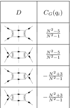
Table 1: Diagrams that contribute to $qq{\rightarrow}qq$ scattering (first column) and gluonic pole strengths of the incoming quarks (second column), where $N$ is the number of colors. For each diagram the gluonic pole strengths of the outgoing quarks are given by $C_{G}(q_{f}){=}{-}C_{G}(q_{i})$.

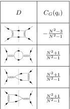
Table 2: Diagrams that contribute to $q\bar{q}{\rightarrow}q\bar{q}$ scattering (first column) and gluonic pole strengths of the incoming quarks (second column). The gluonic pole strengths of the other (anti)quarks are given by $C_{G}(q_{f}){=}C_{G}(\bar{q}_{f}){=}{-}C_{G}(\bar{q}_{i}){=}{-}C_{G}(q_{i})$.

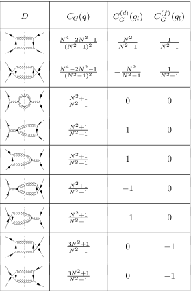
Table 3: Diagrams that contribute to $q\bar{q}{\rightarrow}gg$ scattering (first column) and the gluonic pole strengths of the incoming quarks (second column) and the lower glouns ($g_{l}$) in the final state (third and fourth column). The gluonic pole strengths of the incoming antiquarks and the upper gluons ($g_{u}$) in the final state are connected to those given above through the relations $C_{G}(\bar{q}){=}C_{G}(q)$, $C_{G}^{(d)}(g_{u}){=}{-}C_{G}^{(d)}(g_{l})$ and $C_{G}^{(f)}(g_{u}){=}C_{G}^{(f)}(g_{l})$.

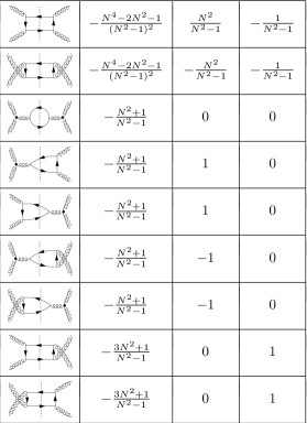
Table 4: Diagrams that contribute to $gg{\rightarrow}q\bar{q}$ scattering (first column) and the gluonic pole strengths of the outgoing quarks (second column) and the lower glouns ($g_{l}$) in the initial state (third and fourth column). The gluonic pole strengths of the outgoing antiquarks and the upper gluons ($g_{u}$) in the initial state are connected to those given above through the relations $C_{G}(\bar{q}){=}C_{G}(q)$, $C_{G}^{(d)}(g_{u}){=}{-}C_{G}^{(d)}(g_{l})$ and $C_{G}^{(f)}(g_{u}){=}C_{G}^{(f)}(g_{l})$.

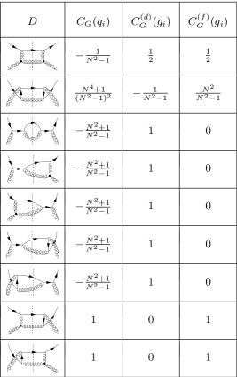
Table 5: Diagrams that contribute to $qg{\rightarrow}qg$ scattering (first column) and the gluonic pole strengths of the incoming quarks (second column) and gluons (third and fourth column). The gluonic pole strengths of the outgoing partons are connected to those given above through the relations $C_{G}(q_{f}){=}{-}C_{G}(q_{i})$, $C_{G}^{(d)}(g_{f}){=}C_{G}^{(d)}(g_{i})$ and $C_{G}^{(f)}(g_{f}){=}{-}C_{G}^{(f)}(g_{i})$.

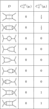
Table 6: The diagrams without 4-gluon vertices that contribute to $gg{\rightarrow}gg$ scattering (first column) and the gluonic pole strengths of the incoming glouns (second and third column). The gluonic pole strengths of the outgoing gluons are connected to those given above through the relations $C_{G}^{(d)}(g_{f}){=}C_{G}^{(d)}(g_{i})$ and $C_{G}^{(f)}(g_{f}){=}{-}C_{G}^{(f)}(g_{i})$.

Table 7: Unpolarized cross sections as defined in section II.

Table 8: Unpolarized gluonic pole cross sections as defined in section II when the gluonic pole is contributed by a quark.

Table 9: Longitudinally polarized cross sections as defined in section II. This reproduces the expressions in Stratmann and Vogelsang (1992) and adds the processes with both polarized partons in the initial or final state.

Table 10: Longitudinally polarized gluonic pole cross sections as defined in section II when the gluonic pole is contributed by a quark.

Table 11: Transversally polarized cross sections as defined in section II. These reproduce the expressions in Bacchetta and Radici (2004), except for an overall sign difference in the processes $q^{\uparrow}g{\rightarrow}q^{\uparrow}g$ and $qg^{\uparrow}{\rightarrow}qg^{\uparrow}$.

Table 12: Transversally polarized gluonic pole cross sections as defined in section II when the gluonic pole is contributed by a quark.

Table 13: Unpolarized gluonic pole cross sections as defined in section II when the gluonic pole is contributed by a gluon.

Table 14: Longitudinally polarized gluonic pole cross sections as defined in section II when the gluonic pole is contributed by a gluon.

Table 15: Transversally polarized gluonic pole cross sections as defined in section II when the gluonic pole is contributed by a gluon.

References

- Adams et al. (1991a) D. L. Adams et al. (E581), Phys. Lett. B261, 201 (1991a).
- Adams et al. (1991b) D. L. Adams et al. (FNAL-E704), Phys. Lett. B264, 462 (1991b).
- Bravar et al. (1996) A. Bravar et al. (Fermilab E704), Phys. Rev. Lett. 77, 2626 (1996).
- Airapetian et al. (2001) A. Airapetian et al. (HERMES), Phys. Rev. D64, 097101 (2001), eprint hep-ex/0104005.
- Adler et al. (2003) S. S. Adler et al. (PHENIX), Phys. Rev. Lett. 91, 241803 (2003), eprint hep-ex/0304038.
- Adams et al. (2004) J. Adams et al. (STAR), Phys. Rev. Lett. 92, 171801 (2004), eprint hep-ex/0310058.
- Airapetian et al. (2005) A. Airapetian et al. (HERMES), Phys. Rev. Lett. 94, 012002 (2005), eprint hep-ex/0408013.
- Belitsky et al. (2003) A. V. Belitsky, X. Ji, and F. Yuan, Nucl. Phys. B656, 165 (2003), eprint hep-ph/0208038.
- Boer et al. (2003) D. Boer, P. J. Mulders, and F. Pijlman, Nucl. Phys. B667, 201 (2003), eprint hep-ph/0303034.
- Collins (1993) J. C. Collins, Nucl. Phys. B396, 161 (1993), eprint hep-ph/9208213.
- Brodsky et al. (2002a) S. J. Brodsky, D. S. Hwang, and I. Schmidt, Phys. Lett. B530, 99 (2002a), eprint hep-ph/0201296.
- Qiu and Sterman (1999) J.-w. Qiu and G. Sterman, Phys. Rev. D59, 014004 (1999), eprint hep-ph/9806356.
- Bomhof et al. (2004) C. J. Bomhof, P. J. Mulders, and F. Pijlman, Phys. Lett. B596, 277 (2004), eprint hep-ph/0406099.
- Bacchetta et al. (2005) A. Bacchetta, C. J. Bomhof, P. J. Mulders, and F. Pijlman, Phys. Rev. D72, 034030 (2005), eprint hep-ph/0505268.
- Bomhof et al. (2006) C. J. Bomhof, P. J. Mulders, and F. Pijlman, Eur. Phys. J. C47, 147 (2006), eprint hep-ph/0601171.
- Collins (2002) J. C. Collins, Phys. Lett. B536, 43 (2002), eprint hep-ph/0204004.
- Brodsky et al. (2002b) S. J. Brodsky, D. S. Hwang, and I. Schmidt, Nucl. Phys. B642, 344 (2002b), eprint hep-ph/0206259.
- Stratmann and Vogelsang (1992) M. Stratmann and W. Vogelsang, Phys. Lett. B295, 277 (1992).
- Vogelsang (1998) W. Vogelsang, Acta Phys. Polon. B29, 1189 (1998), eprint hep-ph/9805295.
- Collins and Metz (2004) J. C. Collins and A. Metz, Phys. Rev. Lett. 93, 252001 (2004), eprint hep-ph/0408249.
- Mulders and Rodrigues (2001) P. J. Mulders and J. Rodrigues, Phys. Rev. D63, 094021 (2001), eprint hep-ph/0009343.
- (22) W. Vogelsang, private communication.
- Boer and Vogelsang (2004) D. Boer and W. Vogelsang, Phys. Rev. D69, 094025 (2004), eprint hep-ph/0312320.
- Anselmino et al. (2006) M. Anselmino, U. D’Alesio, S. Melis, and F. Murgia (2006), eprint hep-ph/0608211.
- Kouvaris et al. (2006) C. Kouvaris, J.-W. Qiu, W. Vogelsang, and F. Yuan, Phys. Rev. D74, 114013 (2006), eprint hep-ph/0609238.
- Gluck et al. (1998) M. Gluck, E. Reya, and A. Vogt, Eur. Phys. J. C5, 461 (1998), eprint hep-ph/9806404.
- Leader et al. (2006) E. Leader, A. V. Sidorov, and D. B. Stamenov, Phys. Rev. D73, 034023 (2006), eprint hep-ph/0512114.
- Hirai et al. (2006) M. Hirai, S. Kumano, and N. Saito, Phys. Rev. D74, 014015 (2006), eprint hep-ph/0603213.
- Thorne et al. (2006) R. S. Thorne, A. D. Martin, and W. J. Stirling (2006), eprint hep-ph/0606244.
- Signal and Thomas (1989) A. I. Signal and A. W. Thomas, Phys. Rev. D40, 2832 (1989).
- Barone and Drago (1993) V. Barone and A. Drago, Nucl. Phys. A552, 479 (1993).
- Jakob et al. (1997) R. Jakob, P. J. Mulders, and J. Rodrigues, Nucl. Phys. A626, 937 (1997), eprint hep-ph/9704335.
- Diakonov et al. (1998) D. Diakonov, V. Y. Petrov, P. V. Pobylitsa, M. V. Polyakov, and C. Weiss, Phys. Rev. D58, 038502 (1998).
- Goeke et al. (2001) K. Goeke, P. V. Pobylitsa, M. V. Polyakov, P. Schweitzer, and D. Urbano, Acta Phys. Polon. B32, 1201 (2001), eprint hep-ph/0001272.
- Gluck et al. (2001) M. Gluck, E. Reya, M. Stratmann, and W. Vogelsang, Phys. Rev. D63, 094005 (2001), eprint hep-ph/0011215.
- Bacchetta et al. (2001) A. Bacchetta, R. Kundu, A. Metz, and P. Mulders, Phys. Lett. B506, 155 (2001), eprint hep-ph/0102278.
- Wakamatsu (2001) M. Wakamatsu, Phys. Lett. B509, 59 (2001), eprint hep-ph/0012331.
- Bacchetta et al. (2002) A. Bacchetta, R. Kundu, A. Metz, and P. Mulders, Phys. Rev. D65, 094021 (2002), eprint hep-ph/0201091.
- Yang (2002) J.-J. Yang, Phys. Rev. D65, 094035 (2002).
- Efremov (2004) A. V. Efremov, Annalen Phys. 13, 651 (2004), eprint hep-ph/0410389.
- Anselmino et al. (1995) M. Anselmino, M. Boglione, and F. Murgia, Phys. Lett. B362, 164 (1995), eprint hep-ph/9503290.
- Anselmino and Murgia (1998) M. Anselmino and F. Murgia, Phys. Lett. B442, 470 (1998), eprint hep-ph/9808426.
- Soper (1977) D. E. Soper, Phys. Rev. D15, 1141 (1977).
- Soper (1979) D. E. Soper, Phys. Rev. Lett. 43, 1847 (1979).
- Ralston and Soper (1979) J. P. Ralston and D. E. Soper, Nucl. Phys. B152, 109 (1979).
- Collins and Soper (1982) J. C. Collins and D. E. Soper, Nucl. Phys. B194, 445 (1982).
- Collins et al. (1982) J. C. Collins, D. E. Soper, and G. Sterman, Phys. Lett. B109, 388 (1982).
- Collins et al. (1983) J. C. Collins, D. E. Soper, and G. Sterman, Nucl. Phys. B223, 381 (1983).
- Jaffe and Ji (1992) R. L. Jaffe and X.-D. Ji, Nucl. Phys. B375, 527 (1992).
- Mulders and Tangerman (1996) P. J. Mulders and R. D. Tangerman, Nucl. Phys. B461, 197 (1996), eprint hep-ph/9510301.
- Bacchetta and Radici (2004) A. Bacchetta and M. Radici, Phys. Rev. D70, 094032 (2004), eprint hep-ph/0409174.